Revisiting Query Performance in GPU Database Systems

Abstract.

GPUs offer massive compute parallelism and high-bandwidth memory accesses. GPU database systems seek to exploit those capabilities to accelerate data analytics. Although modern GPUs have more resources (e.g., higher DRAM bandwidth) than ever before, judicious choices for query processing that avoid wasteful resource allocations are still advantageous. Database systems can save GPU runtime costs through just-enough resource allocation or improve query throughput with concurrent query processing by leveraging new GPU capabilities, such as Multi-Instance GPU (MIG).

In this paper we do a cross-stack performance and resource utilization analysis of five GPU database systems. We study both database-level and micro-architectural aspects, and offer recommendations to database developers. We also demonstrate how to use and extend the traditional roofline model to identify GPU resource bottlenecks. This enables users to conduct what-if analysis to forecast performance impact for different resource allocation or the degree of concurrency. Our methodology addresses a key user pain point in selecting optimal configurations by removing the need to do exhaustive testing for a multitude of resource configurations.

1. INTRODUCTION

Graphics Processing Units (GPUs), with their potential for massively parallel computing, high-bandwidth memory access capability, and relative easy of programming for an accelerator, have seen rising interests in their usage for accelerating data analytics, with a number of GPU database systems being developed in both academic and industrial settings in recent years (He et al., 2022; BlazingSQL, 2021; HeavyDB, 2022; Shanbhag et al., 2020; Kohei, 2022; Bakkum and Chakradhar, 2010; Shen et al., 2019; Krolik et al., 2021; Paul et al., 2016; Funke et al., 2018; Heimel et al., 2013; Wu et al., 2014; Floratos et al., 2021). Recent advances in interconnect protocols (pci, 2017, 2019, 2022b, 2022a) and architectural enhancements have made GPUs more attractive as accelerators for data analytics, and we expect an increase in the popularity of GPU database systems and a proliferation of research into improving their efficiency going forward.

Query performance in GPU database systems depends on several factors: (1) the computational capacity of the GPU, (2) the implementation of the query execution engine, (3) the characteristics of the query, and (4) the database size. A deeper understanding of GPU resource utilization and bottlenecks encountered is important for designing better GPU database systems.

Prior Work. While previous studies (e.g., (Furst et al., 2017; Suh et al., 2022; He et al., 2022)) have compared query performance across GPU database systems, a cross-stack analysis that connects query processing design choices with the impact on micro-architectural performance metrics is missing—conversely similar studies (Ailamaki et al., 1999; Sirin and Ailamaki, 2020; Sen and Ramachandra, 2018) exist for CPU database systems. We aim to address this gap in this paper, and develop recommendations for GPU database developers and hardware vendors.

Cloud GPUs. Several GPU instance types are now available on the cloud: from GPUs well fitting ML inference workloads (e.g., NVIDIA T4), to more powerful GPUs for ML training (e.g., P100, V100), to high-end one such as the A100. Each of such GPUs have different performance/cost trade offs which are widely unexplored for database workloads. For example, a T4 GPU can run the TPC-H benchmark 20% slower compared to a P100, but at $\frac{1}{5}$ of the cost (He et al., 2022). To complicate things further, starting from the Ampere generation, NVIDIA now allows different resource allocations strategies through the Multi-Instance GPU (MIG) capability (NVIDIA, 2022a). This new capability allows to partition GPU hardware resources to either increase concurrency, or decrease the cost by sharing resources. For instance, Figure 1 shows the query execution time and GPU resource trade-offs for running representative queries from the Star Schema Benchmark (SSB) (Rabl et al., 2013) using HeavyDB (an open-source GPU database system (HeavyDB, 2022)) on an NVIDIA A100 GPU with MIG. We observe that query performance does not always scale linearly with respect to the allocated GPU resources. For example, performance of memory-bound kernels that under-utilize DRAM bandwidth may remain unaffected with less allocated bandwidth. The scaling characteristics depend both on the data size (Figure 1(a)) and query properties (Figure 1(b)). In summary, developers are now offered with several choices on how to schedule their workloads over GPUs, but these choice are not trivial, and requires a deep understanding of both workloads characteristics and hardware properties.

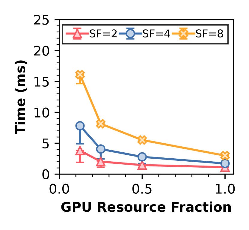
(a) Same query (Q33) with different SFs.

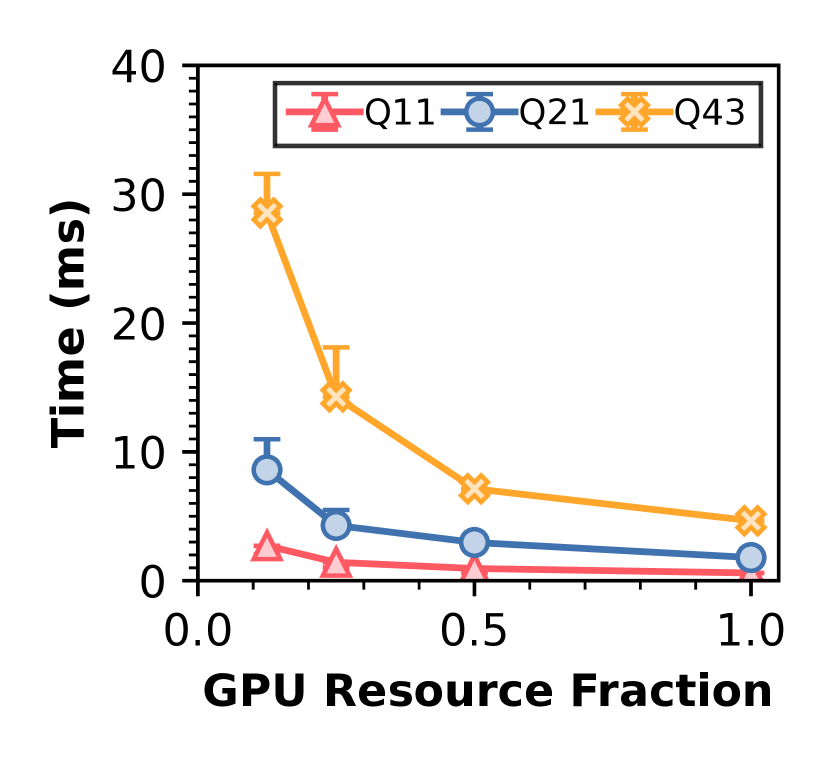
(b) Different queries with same SF=4.

Figure 1. Query Execution Time (and Estimation Error) vs. Resource Allocation – Query execution time vs. GPU resource allocations for representative queries (§ 3.2) and scale factors (SFs), along with the error of the time estimates (shown with bars) using our predictive framework. X-axis denotes the fraction of GPU resources being used to run the queries.

Modeling to the rescue. To solve the above problem, currently users must rerun representative workloads with different allocations and then choose the most suitable configuration. This is a tedious and expensive process. In this paper we propose an analysis framework based on roofline models (Williams et al., 2009)— a widely used tool for analyzing bottlenecks. Our analysis framework automatically estimates the resource-performance trade-offs of database systems on GPUs to guide users in making informed decisions about resource allocations with small errors (shown by bars in Figure 1). Using this framework, we discover that database queries often under-utilize GPU resources. We uncover an opportunity to improve overall GPU utilization and workload performance by exploiting concurrent execution—our results show speedups of up to $6.43\times$ by using our framework to select the optimal degree of concurrency. Finally, our modelling framework outperforms state-of-the-art (SoTA) white-box analytical model, by leveraging runtime statistics from prior executions of queries (which often occurs in practice in analytical workloads (Jyothi et al., 2016; Sen et al., 2020)).

Contributions. The key contributions of this work are:

• Comparative Analysis of GPU database systems (§ 4): We compare performance of queries in five GPU database systems from both database and micro-architectural perspectives. We find that lazy result caching, avoiding unnecessary algorithmic complexity, and eliminating unnecessary materialization of intermediate results are important for improving query performance.

• Performance Modeling (§ 5): We explore modeling query performance for two scenarios: data size change and resource change. For the first scenario, we significantly improve upon a SoTA model (Crystal) for recurring queries by incorporating more realistic assumptions about memory resource utilization, which include both caches and DRAMs. For the second scenario, we present a roofline model that is effective in identifying and visualizing bottlenecks. The efficacy of the model stems from its consideration of L2 cache bandwidth along with the traditional memory bandwidth and compute resource bottlenecks.

• Model-Driven Resource Management and Scheduling (§ 6): We demonstrate that our framework is able to predict workload performance at different resource allocations and degrees of concurrency. We will show how users and system administrators can automatically derive cost-performance trade-off estimates for various scheduling scenarios, eliminating the need for re-running the workload under a multitude of configurations.

2. GPU DATABASE SYSTEMS

In this section, we provide an overview of the GPU database systems that we are going to examine in this paper. Table 1 summarizes the key characteristics of these five database systems (Shanbhag et al., 2020; HeavyDB, 2022; BlazingSQL, 2021; He et al., 2022; Kohei, 2022). These systems range from Crystal, a highly-optimized academic prototype with limited query coverage, to HeavyDB, a production-grade system that supports a broader range of queries.

Table 1. Qualitative comparison of GPU database systems – We consider the following characteristics. Coverage: whether the system is general purpose or only specific queries are supported. Data Format: formats for data input to the system. Backend: how data operators are compiled for execution. Execution: whether operators are executed on GPU or both on CPU and GPU. Open Source: if the system is publicly available.

System	Crystal	HeavyDB	BlazingSQL	TQP	PG-Strom
Coverage	SSB (O’Neil et al., 2009) only	General purpose	General purpose	General purpose	Join Aggr.
Data Format	Binary array	CSV Parquet	CSV, DF Parquet	CSV, DF Parquet	CSV
Backend	Hardcoded CUDA	LLVM to PTX	Thrust cuDF	PyTorch	CUDA
Execution	GPU	GPU	GPU	GPU	CPU+GPU
Open Source	Yes	Yes	Yes	No	Yes

Crystal. Crystal (Shanbhag et al., 2020) is a recently proposed SoTA GPU database system that delivers superior query execution performance compared to other systems. However, the types of queries that it supports are limited. It currently only supports queries from the Star Schema Benchmark (SSB) (O’Neil et al., 2009). All the queries are written in CUDA, and they have hard-coded parameters for the size of the hash table, the number of groups, and the size of the output table (Shanbhag, 2020). While this is feasible for these queries in SSB, it is not feasible to pre-determine these parameters for arbitrary SQL queries. Crystal also assumes that each column is a binary array generated during the pre-processing phase. If a column contains string values, this is converted to a binary array using dictionary encoding. This encoding process happens in CPU before query execution.

HeavyDB. HeavyDB (HeavyDB, 2022) is a widely-used GPU database system that supports many types of SQL queries. Besides the query executor, it contains other components like query parser and query optimizer. HeavyDB takes various data formats as input, such as CSV and Parquet. Internally, it uses LLVM (Lattner and Adve, 2004) to generate PTX (NVIDIA, 2022d) to build the query execution. Additionally, HeavyDB leverages a custom LLVM pass for more flexible and optimized execution strategies. Though HeavyDB currently only supports NVIDIA GPUs, it can be extended to other hardware platforms using LLVM.

BlazingSQL. BlazingSQL (BlazingSQL, 2021) is another open-sourced GPU database system. Similarly to HeavyDB, BlazingSQL is also very flexible and handles different types of queries. Unlike HeavyDB, it uses Thrust (NVIDIA, 2022e) and cuDF (Team, 2018) as its backend for query execution. Reusing the APIs of Thrust and cuDF has both pros and cons. While less engineering is needed to support various operations, due to limited functionalities of existing APIs, certain operators cannot be implemented in an efficient way (e.g., cannot avoid unnecessary generation of intermediate results). BlazingSQL also supports different input data formats.

PG-Strom. PG-Strom (Kohei, 2022) is an extension to the widely-used PostgresSQL database system. It supports offloading of some operators, such as join and aggregation, to the GPU. PG-Strom uses CUDA as its implementation backend. The unique characteristic of PG-Strom is that it executes queries across both CPU and GPU. This allows the extension to be very general-purpose since it can always fall back to CPU execution. On the other hand, this approach also leads to sub-optimal performance due to the overhead of data movement between CPU and GPU (as we will see shortly). Except for PG-Strom, all the other GPU database systems that we consider are designed for GPU-only query execution where tables are lazily cached in the GPU device memory to avoid table movement overhead during query execution.

TQP. TQP (He et al., 2022) is a recently presented GPU database system from Microsoft. It is designed to be general purpose (e.g., it supports the full TPC-H benchmark). The interesting aspect of TQP is that internally it uses the PyTorch (Paszke et al., 2019) framework as its backend for executing relational operations. This design choice allows it to quickly support many different operations with existing GPU kernels that are already optimized. As the PyTorch framework already supports various hardware platforms (e.g., NVIDIA GPUs, AMD GPUs), TQP inherits the portability and extensiblity of the PyTorch framework.

Query Optimization in GPU Database Systems. All the systems have query optimization and query compilation phases except for Crystal: here the query plans are hard-coded and pre-determined based on the selectivity of each operator (i.e., selective operators are executed earlier). HeavyDB and BlazingSQL rely on the Apache Calcite framework for query optimization. After query optimization, HeavyDB uses LLVM to compile the query plans, and also uses LLVM to further optimize the physical execution of GPU code. In contrast, BlazingSQL constructs the physical query plan using Thrust and cuDF libraries.

TQP uses SparkSQL (Armbrust et al., 2015) to optimize the SQL queries, and then translates the Spark SQL physical plans to an intermediate representation (IR). Based on the IR, TQP assembles a PyTorch program as a composition of pre-defined tensor programs, one for each operator in the IR. The implementation is later optimized by the PyTorch compiler. PG-Strom takes a different approach since it directly leverages the PostgreSQL query optimizer. Specifically, it leverages a GPU-aware cost model that allows the GPU execution to be a part of the PostgreSQL query optimization phase. Based on the relative cost, the optimizer determines which operators to offload to GPU. This approach requires the optimizer to have a good estimate of the cost of each operator in the query plan.

3. EXPERIMENTAL SETUP

We go over the hardware, query workloads, and profiling toolchains used in this paper in § 3.1, § 3.2 and § 3.3, respectively. We then describe the two execution scenarios that we consider in § 3.4.

3.1. Hardware

We use an NVIDIA A100 GPU (NVIDIA, 2020) with Ampere GPU architecture, $40$GB of GPU memory, and $108$ Streaming Multiprocessors (SMs). NVIDIA GPU hardware operates at the warp granularity. A warp consists of $32$ threads scheduled and executing together in a single instruction, multiple threads (SIMT) fashion (i.e., each thread executes the same instruction on different data but allowing divergence between threads). Each SM can schedule up to 64 warps. The A100 GPU supports newer features like multi-instance GPU (NVIDIA, 2022b). We will provide more information on this feature in § 6.1. The GPU is connected to the CPU via PCI-e $4$ protocol, which provides up to $32$ GB/s of bandwidth. To achieve consistent performance, we lock the GPU clock frequency at $1410$ MHz.

3.2. Workloads

Since Crystal currently only supports SSB (O’Neil et al., 2009), in our experiments we decided to evaluate the SSB benchmark over the five different GPU database systems. Even if SSB is simpler than other benchmarks like TPC-H and TPC-DS, its queries are complex enough that system characterization on this benchmark enables us to find several interesting insights. We are confident that these insights generalize to other workloads as well.

Table 2 presents a summary of the queries in the SSB benchmark. Queries in group $1$ only have one join, and the results are aggregated into a single scalar value. All the other queries have multiple joins (up to 4), and the final results are aggregated into a table with multiple groups. Based on our profiling, we found that $16$ is the largest scale factor that most database systems support without running into out-of-memory errors. So, we only present results up to scale factor $16$, whose tables sizes are near $7$ GB.

Table 2. Qualitative summary of the queries from the SSB benchmark – Key characteristics of queries in the SSB benchmark: Number of Joins, the Aggregation type, whether they require Sorting, and query Selectivity.

Query Group

Group 1

Group 2

Group 3

Group 4

Q11

Q12

Q13

Q21

Q22

Q23

Q31

Q32

Q33

Q34

Q41

Q42

Q43

# Joins

$1$

$3$

$3$

$4$

Aggregation

Sum

Group By

Group By

Group By

Sorting

No

Yes

Yes

Yes

Selectivity

1.9e-2

6.5e-4

7.5e-5

8e-3

1.6e-3

2e-4

3.4e-2

1.4e-3

5.5e-5

7.6e-7

1.6e-2

4.6e-3

9.1e-5

3.3. Profiling Toolchains

We extensively use NVIDIA Nsight System (NVIDIA, 2022c), Nsight Compute (NVIDIA, 2022c), and nvidia-smi (NVIDIA, 2016) tools. NSight System provides system-wide time breakdown, including time spent on data transfer, memory allocation, kernel execution, etc. However, we cannot study the kernel execution efficiency only based on those high-level metrics, and that information is needed for query performance modeling. Thus, we also use Nsight Compute to obtain detailed kernel execution metrics, which includes achieved instruction per cycle, cache utilization, etc. Nvidia-smi allows power monitoring.

3.4. Warm vs. Cold Execution Scenarios

We consider two execution scenarios for performance characterization: warm and cold. With the warm scenario, we assume that the data has been already loaded (or cached) in GPU memory, the device has been already warmed up, and the query has been already parsed, optimized, and compiled (e.g.,, the physical plan is available in the plan cache). With the cold scenario, we assume that the data resides in CPU memory and needs to be transferred to the device, and we consider all the other overheads associated with query parsing, optimization, and compilation.

4. PERFORMANCE ANALYSIS

We next characterize the performance of different database systems on the A100 GPU. Along with the results, we also highlight the key insights obtained from these experiments. We show insights for cold and warm query execution in § 4.1 and § 4.2, respectively. Afterwards, in sections 4.3, 4.4, 4.5 we provide a deeper analysis of where the time is spent during the GPU execution. Finally, in § 4.6 we provide a brief overview of the kernel implementation efficiency.

4.1. End-to-End Cold Query Execution

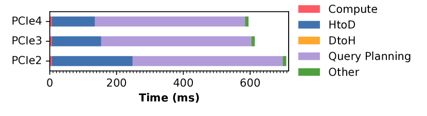
Figure 2. Cold execution characterization over Q21 at SF=16 in HeavyDB – We split the end-to-end performance of cold query execution into six components: Compute time, Host to Device data transfer (HtoD), Device to Host data transfer (DtoH), Query Planning time, and Other CUDA context setup and memory management time. Similar results apply for other queries and database systems.

With cold query execution, besides actual query execution, there are several non-negligible overheads from both query optimization and compilation, and data transfer. Figure 2 shows that these overheads are always greater than the overhead of the actual query execution. As data needs to be moved to the GPU before query execution, the data transfer operation incurs a significant overhead. During data transfer, it is not optimal to naively copy over all columns of the table. Instead, most systems only copy the columns needed for the query to GPU, which reduces the host to device data transfer overhead. HtoD overhead in Figure 2 reflects the time spent on copying the required columns.

Systems also need to move results from the device back to the host. However, as all the queries compute aggregated results that are very small in size, the device to host overhead is minimal in general. Query plan optimization and compilation also introduces non-trivial overheads. This is unavoidable when the system receives a query for the first time. Most systems implement plan caching, so recurrent queries do not have the same overhead. Lastly, we observe that the evaluated GPU database systems do not fully utilize the PCIe4 bandwidth. While running the database systems over PCIe3demonstrates significant benefit over PCIe2, we found through our profiling that the benefit of moving from PCIe3 to PCIe4 is smaller because of the under-utilization of the PCIe bandwidth. Additionally, we found that the achieved data movement bandwidth drops when the table size does not fit into GPU DRAM capacity, because both input data and results need to streamed in and out GPU during query execution. ✝ Finding. Selectively transferring and caching columns to GPU, as well as plan caching, are beneficial to both cold and warm query execution.
✽ Recommendation. Improving the effective data movement bandwidth will further boost query execution performance.

4.2. End-to-End Warm Query Execution

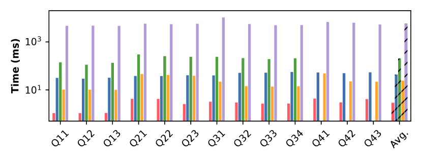
Figure 3. Warm execution characterization – End-to-end performance for all queries (BlazingSQL does not support queries in group 4).

We show the end-to-end warm query execution performance in Figure 3 . The most notable observation is that Crystal represents the upper bound in execution performance among all considered systems. HeavyDB is on average $15\times$ slower than Crystal and TQP is $8\times$ slower than Crystal. BlazingSQL and PG-Strom are even slower. They are $71\times$ and $2022\times$ slower than Crystal, respectively. Next, we provide more in depth analysis on the end-to-end warm query execution of each system.

Crystal and TQP. For these both systems, the end-to-end time only reflects the actual GPU compute time. In Crystal, each CUDA source file implements one query from SSB. Once the source file is compiled, there is no additional compilation overhead associated with the query. Unlike Crystal, TQP is a general-purpose system that supports a wider range of SQL queries. In TQP the workflow for executing queries is done in two phases: the input query is first parsed, optimized and compiled into a PyTorch model object; then the already-compiled model is executed over the input data. Because to this workflow, the query execution time does not contain optimization and compilation time. In addition, TQP lazily caches the query results in GPU, until it is requested by the user. This approach is beneficial in reducing end-to-end query execution time if the results are not immediately required, or if there is a subsequent query executing on the previously generated output results.

HeavyDB and BlazingSQL. For HeavyDB and BlazingSQL, their reported end-to-end time not only consists of the GPU compute time, but also includes other overheads. For example, HeavyDB uses Calcite for query plan optimization, and LLVM to compile the query into executable code. Since HeavyDB implements a plan cache, we expected it to have negligible overhead for both optimization and compilation. However, in reality, that is not the case. Similar to HeavyDB, BlazingSQL also has non-trivial overheads beyond the GPU compute time. This observation motivates us to study only the GPU compute time of the database systems in § 4.3.

PG-Strom. Compared to other systems, PG-Strom has a very high end-to-end query execution time. The reason is because of its CPU-GPU co-execution design. In PG-Strom, operators are partially executed on CPU and partially executed on GPU. PG-Strom needs to transfer the intermediate results from CPU to GPU or from GPU to CPU if the execution platform changes. Due to the design of its execution engine, it is challenging to implement lazy data caching mechanism like other systems, because the intermediate results will rarely be reused (as they are query-specific).

✝ Finding. ❶ Several systems show overheads beyond the GPU query execution time. ❷ PG-Strom implements some operators in CPU forcing CPU+GPU co-execution.
✽ Recommendation. ❶ Minimizing warm execution overheads can be major source of optimization opportunities. ❷ CPU+GPU execution should be chosen carefully considering data transfer overhead. ❸ Lazily copying of the query results in CPU memory can avoid unnecessary data movement overhead.

4.3. GPU Compute Time

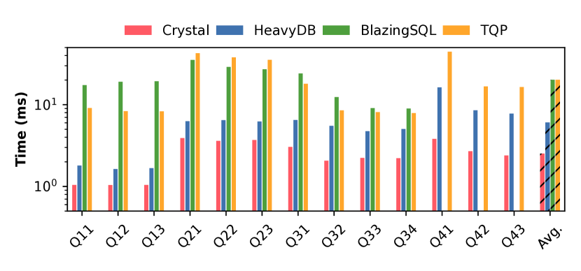
Figure 4. GPU compute time characterization – compared to the end-to-end warm execution of Figure 3, HeavyDB and BlazingSQL performance improve compared to Crystal, while TQP performance decreases.

Following the observation made in § 4.2, we study the overheads of the GPU execution, for each of the considered systems. Because PG-Strom only partially execute query plans in GPU, we do not include PG-Strom in this analysis and subsequent experiments. The GPU compute time of the studied systems is reported in Figure 4.

As expected, Crystal is still the fastest system. However, unlike the end-to-end query time, if we only consider the GPU execution efficiency, HeavyDB is very close to Crystal ($2\times$ slowdown as opposed to $15\times$ slowdown reported in end-to-end comparison § 4.2). TQP is still $15\times$ slower than Crystal. So, HeavyDB is now around $4\times$ faster than TQP. TQP has very similar GPU compute performance to BlazingSQL. In next section, we conduct a deeper analysis of why these systems vary in their GPU execution performance.

✝ Finding. Systems have dramatically different GPU compute efficiency compared to results demonstrated in end-to-end query execution time.

4.4. GPU Execution Efficiency

We study the warm GPU execution efficiency by profiling these hardware counters: (1) the number of integer operations, and (2) bytes loaded from DRAM.

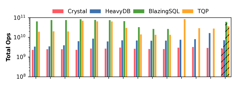
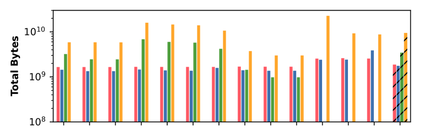
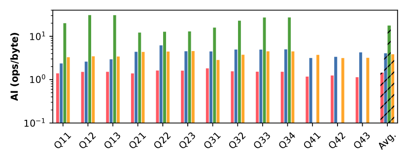
Figure 5. GPU execution efficiency – total integer operations (top), number of bytes from DRAM (middle), and arithmetic intensity (bottom).

Integer Operations. We first profile the total integer operations for the four systems, as shown in Figure 5 (top chart). We find that HeavyDB does slightly more integer operations than Crystal. This is expected because HeavyDB is designed to be more flexible and supports generic queries. For example, it has GPU algorithms to calculate hash-table sizes on-the-fly, while Crystal has a hard-coded hash-table size. On the other hand, BlazingSQL and TQP uses significantly more integer operations compared to Crystal and HeavyDB. This is because those two systems have more complicated implementations, and they do not fuse operators. For instance, BlazingSQL implements a very complex MurmurHash algorithm to distribute keys more evenly.

Bytes. Next, we look into the number of bytes each system reads from the GPU device memory (Figure 5, middle chart). Similar to number of integer operations each system operates, Crystal and HeavyDB also read less data from GPU device memory than other two systems. We credit this to operator fusion, which allow both systems to read and materialize the minimal amount of data. On all queries, Crystal reads slightly more data from GPU than HeavyDB due to its bulk execution model. On the other hand, BlazingSQL and TQP generate many intermediate results, since they generate new columns after each query operator. So, they read significantly more data from GPU DRAM in most of the cases. An exception is for queries Q32, Q33, and Q34, where the amount of data loaded from GPU DRAM by BlazingSQL is equal to or even lower than Crystal and HeavyDB. Our investigate reveals that Crystal does not fully avoid unnecessary data loading after predicates.

Arithmetic Intensity. Arithmetic intensity (AI) is a critical metric for modeling the performance of a query (number of operations divided by number of bytes read). In Figure 5 (bottom chart), we show the derived AI of the four systems. The result suggests that Crystal, HeavyDB, and TQP have very similar AI. In other words, all three systems perform a similar number of arithmetic operations for the same amount of data. But, BlazingSQL is much more compute bound on average (around $5\times$ higher AI).

✝ Finding. ❶ Number of integer operations and number of bytes read are key indicators of in-GPU execution efficiency. ❷ OLAP queries can be either compute-bound or memory-bound depending on the implementation.
✽ Recommendation. Reducing number of bytes read by enhancing data reuse and avoiding unnecessary algorithmic complexity can improve GPU execution efficiency.

4.5. Warp Execution Efficiency

The advantage GPU is that it is able to hide different types of execution stalls with its massive parallelism. If a warp $x$ encounters stall due to memory request, the GPU quickly schedules another warp $y$ for execution, so that the memory stall of $x$ is hidden. This approach improves the number of executed instructions per cycle. A warp may stall during execution due to various reasons. Investigating warp execution efficiency allows us to better understand which resource bottlenecks the GPU. Specifically, we obtain a breakdown of stalls associated with warps across systems.

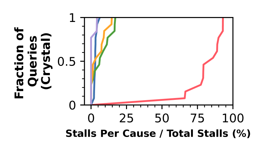
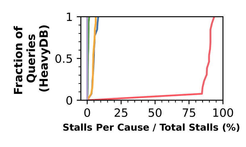
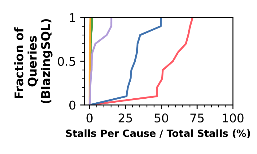
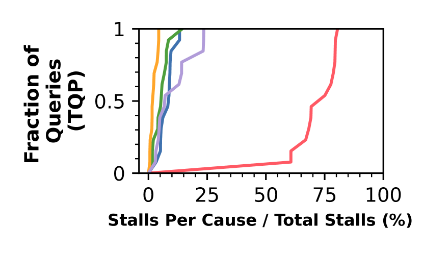
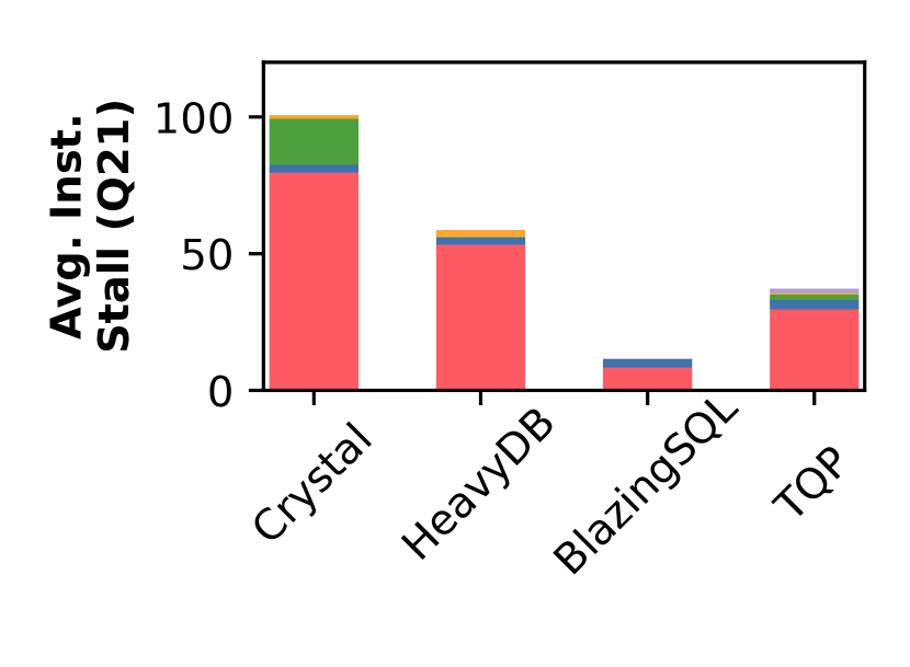
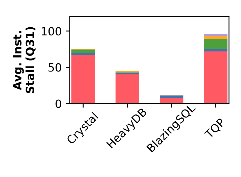
Figure 6. Analysis of Stalls – Stall distribution of all queries and detailed stall breakdown for two queries across all database systems. We only report the top five stall causes (other causes are very rare). Mem LD: stall for memory load request to complete. Compute: stall for fixed latency arithmetic operation to finish. Mem Queue Full: pending memory requests reach maximum. Mem WB: stall for results to write back to memory. Branch: stall due to control-divergent execution.

Figure 6 shows the cumulative distribution functions (CDFs) of stall breakdowns for all SSB queries. To further understand the differences between the systems, we pick two representative queries and show their detailed stall breakdown (Q21 and Q31). All other queries have stall breakdown trends similar to Q21, in which Crystal has the highest stalls, HeavyDB and TQP have lower stalls, and BlazingSQL always has the lowest stalls. Stall breakdown of Q31 is the only exception, where TQP has the highest stall compared to other due to large intermediate results for less selective query (§ 3.2). In both stall breakdown results, BlazingSQL consistently has the lowest average number of warps stalled due to memory requests. This indicates that complicated algorithms can tradeoff memory stall with arithmetic stall, but is not beneficial for overall query performance. TQP tends to have more stalls when the query is less selective (i.e., more rows needs to be materialized).

✝ Finding. ❶ Warp stall is mostly caused by memory requests. ❷ Using complicated algorithms ameliorates memory stalls, but does not improve overall performance.

4.6. Time-Consuming Kernels

Table 3. Summary of most time-consuming kernels – three most time-consuming GPU kernels for executing query Q21 between all systems.

		Top 1	Top 2	Top 3
Crystal	Kernel	probe_ht	build_htp	build_hts
	Time (ms)	3.96 (99.35%)	0.01 (0.37%)	0.01 (0.37%)
HeavyDB	Kernel	multifrag	fill_hj	init_hj
	Time (ms)	5.86 (91.78%)	0.51 (7.96%)	0.01 (0.19%)
BlazingSQL	Kernel	probe_ht	comp_hj_output	parallel_fn
	Time (ms)	13.42 (38.26%)	12.27 (34.97%)	5.55 (15.83%)
TQP	Kernel	collect_fn	idx_select	gather_fn
	Time (ms)	16.88 (40.88%)	9.55 (23.13%)	5.72 (13.86%)

Lastly, we report a GPU compute-time breakdown for query Q21 over the four systems. Interestingly, we found that the time breakdown between different queries is very consistent, therefore here we only show the results of query Q21. We only report the three most time-consuming kernels due to space limitation. We note that BlazingSQL and TQP run $172$ and $190$ kernels, respectively.

Crystal and HeavyDB. These systems spend most of the query execution time in only the top kernel. As shown in Table 3, more than $90\%$ of the total compute time is spent on the top kernel. This is because both systems implement kernel fusion, through which they execute as many operators from the query in a kernel as possible to avoid generation of intermediate results. Because only the hash-join operation is a pipeline breaker (Neumann, 2011) for this particular query, they implement the hash-join build phase in a separate kernel (e.g., build_htp and fill_hj).

BlazingSQL. In this case, one query is split into many kernels. Between the different kernels, generated data (e.g., bitmap to indicate selected rows) needs to be materialized in order to be visible to other kernels. This causes higher overhead compared to other systems that do not need to materialize the intermediate results. Results show that even the hash-table probing phase already exceeds the execution time of both Crystal and HeavyDB.

TQP. Similar to BlazingSQL, TQP also executes many kernels to finish one query, and in fact it spends more time on intermediate results materialization than on actual query execution. For example, according to the documentation from PyTorch, idx_select function (second kernel) indexes a tensor to create a new tensor. It is used to create a new column after each predicate, but its overhead is very high compared to other kernels. Creation of intermediate results not only causes storage overhead due to the limited GPU device memory space, but it is also costly for the entire query execution.

✝ Finding. ❶ Systems with good performance require minimal number of kernels for a query. ❷ Column materialization after predicate evaluation is very expensive. It may have even higher overhead than query operators.
✽ Recommendation. Systems can improve performance through kernel fusion to avoid generation of intermediate results.

5. PERFORMANCE MODELING

The performance analysis so far is based on runtime metrics observed for a given execution of the queries with a fixed input size and GPU resource allocation. However, such analyses are unable to project performance or analyze scalability in unseen scenarios (e.g., different input size or resource allocation). Performance models are essential tools that enable such analyses, in addition to providing additional insights into performance bottlenecks.

In this section we present two models — a white-box model (§ 5.1) that is dependent on the implementations of query operators and it can estimate query performance for input size changes; and a black-box model (§ 5.2) that is agnostic of the query implementation details, and it can predict query performance for GPU resource allocation changes.

5.1. White-Box Model (Crystal)

Crystal (Shanbhag et al., 2020) proposes a white-box model for estimating query performance on GPUs. It assumes that memory bandwidth is the only potential bottleneck for OLAP query execution on GPUs, so performance are proportional to the GPU memory peak bandwidth in this model. For example, the runtime of doing simple projection of an $int32$ column with N rows can be estimated as follows. This model may be extended to other operators like hash join. For example, the runtime of probing an $int32$ column with N keys in a $60$ MB hash-table on the A100 GPU (whose L2 cache size is $40$ MB) can be estimated as follows.

(1) $$\frac{4\cdot\mathrm{N}}{\mathrm{Bandwidth_{\scaleto{DRAM}{4pt}}}}+\frac{(1-\frac{40}{60})\cdot 4\cdot\mathrm{N}}{\mathrm{Bandwidth_{\scaleto{DRAM}{4pt}}}}$$

The left and right terms represent the time taken to load the probe table and to probe the hash-table, respectively. $1-\frac{40}{60}$ indicates the potential miss rate when the kernel probes the hash-table.

Figure 7 shows that depending on the query and scale factor, the errors of the Crystal model can be large. For example, Q11 in Crystal only has a scan. So the absolute difference between estimated and actual time is small. But, on queries with joins, such as Q21 and Q41, the gap between estimated and actual time is large.

Improving the Model for Recurring Queries. A reason for this gap in Crystal is that it does not account for less-than-full bandwidth utilization of DRAM and cache. We improve the model by providing higher accuracy for warm recurrent queries by utilizing run-time statistics from previous executions.

We illustrate our improved model, Crystal-Opt, using two examples. For simple projection queries, we add DRAM utilization factor (obtained from performance counter) into the equation:

(2) $$\frac{4\cdot\mathrm{N}}{\mathrm{Bandwidth_{\scaleto{DRAM}{4pt}}}\cdot\mathrm{Utilization_{\scaleto{DRAM}{4pt}}}}$$

To model the runtime of hash-join probing, since the first term in Equation 1 is for the projection, so we add the utilization factor to improve it (as Equation 2). We then improve the second term (i.e., hash-table probing) in Equation 1 as follows:

$$(1 -\mathrm{HitRate_{\scaleto{L1Cache}{4pt}}})\cdot\frac{\mathrm{Cacheline_{\scaleto{L1Cache}{4pt}}}\cdot\mathrm{N}}{\mathrm{Bandwidth_{\scaleto{L2Cache}{4pt}}}}$$

$$+(1-\mathrm{HitRate_{\scaleto{L2Cache}{4pt}}})\cdot\frac{\mathrm{Cacheline_{\scaleto{L2Cache}{4pt}}}\cdot\mathrm{N}}{\mathrm{Bandwidth_{\scaleto{DRAM}{4pt}}}}$$

We consider the L1 hit rate (assuming its latency is negligible) first. We calculate the L2 access latency based on that. Then, we calculate total data accesses to GPU DRAM considering hit rates of L1 and L2 caches. A limitation of our model is that we need to profile the query once to obtain those performance counters (e.g., L1 and L2 cache hit rates) to predict for other scale factors. In contrast, the original Crystal model does not require any profiling.

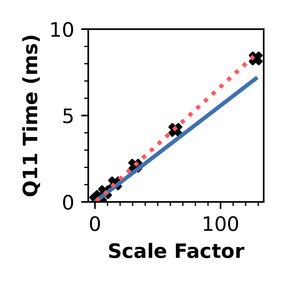
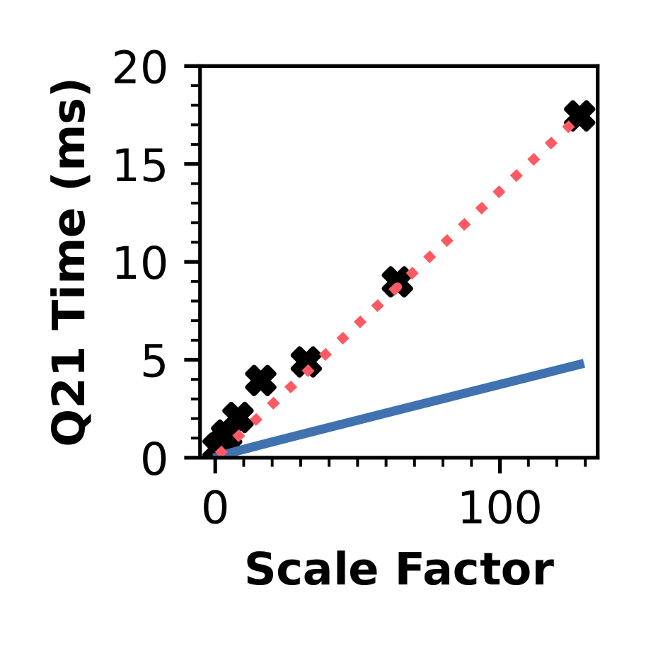
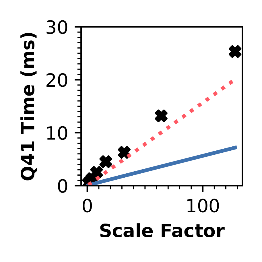
Figure 7. Estimation Time Comparison – Actual query execution time and estimated query execution time of Crystal and Crystal-Opt models.

Figure 7 shows the improvement in prediction accuracy for the selected queries. For these predictions, we use the performance counters from a previous run with SF=16. For Q11, the improvement is small because Crystal implements it using scan and filter operations, which easily saturate the DRAM bandwidth. Taking DRAM utilization into consideration does not have significant benefits. However, for Q21 and Q41, Crystal-Opt shows smaller error (max of $4.8\times$) compared to the Crystal model. The error tends to increase for our improved model for very small or large SFs. This is because we only profile performance counters once and project it to queries with different SFs, leading to less accurate estimates. If additional profiling cost can be tolerated, the error of our improved model will further decrease.

While white-box models give insights into how individual operators contribute to query execution time, they are specific to a given database system. The Crystal model only applies to Crystal and it is tedious to develop a new model for each DBMS. The Crystal model also does not consider bottlenecks due to hardware resources other than memory bandwidth. Now that we have shown that resources may often be under-utilized, we seek to model utilization of GPU resources for different queries and different systems.

✝ Finding. Memory bandwidths are under-utilized.

5.2. Black-Box Model (Roofline)

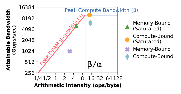
Figure 8. Roofline Model with different resource bounds.

The roofline model (Williams et al., 2009) assumes that any execution on a specific hardware is bounded either by its memory resources or its compute resources. Visually, as shown in Figure 8, the model contains two lines to indicate the peak memory bandwidth ($\alpha$) and the peak compute bandwidth ($\beta$). All executions on this particular hardware will correspond to points within the space bounded by these lines—those two lines are considered as the performance ceilings for that hardware. The X-axis represents the arithmetic intensity (AI), calculated by dividing the total number of operations (e.g., integer or floating-point operations) by the total number of bytes read during execution. The Y-axis indicates the achieved throughput, calculated as the executed operations per second.

Conventionally, a query could be either memory-bound (AI $<$ $\frac{\beta}{\alpha}$), or compute-bound (AI $>$ $\frac{\beta}{\alpha}$)  (Ofenbeck et al., 2014). The performance of algorithms that already saturate the bandwidth of either of those resources will be impacted by changes in allocation of the corresponding resource (e.g., memory-bound saturated or compute-bound saturated in Figure 8). Algorithmic or compiler inefficiencies will increase the AI and make an otherwise memory-bound execution compute-bound, with the query taking more time to complete. However, we show that it is important to consider L2 cache bandwidth as an additional bound for query executions in GPUs, and that compute-bound executions are impacted by changes in compute resource allocations.

Case Study.

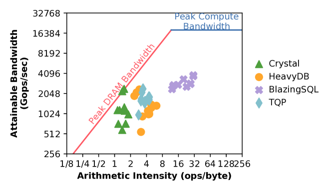
Figure 9. DRAM Roofline Model – for SSB queries (SF=16).

We now present our performance modeling results over the four systems in Figure 9. We obtain the metrics described in Table 4, from which we derive the AI and the attainable bandwidth. We use the theoretical GPU DRAM bandwidth (NVIDIA, 2020) for the DRAM bandwidth ceiling. We note that GPUs also have other functional units like floating-point operations unit. However, because most OLAP queries only require integer operations, those functional units are not needed for constructing the roofline model.

The challenge for this type of modeling is that each query consists of multiple kernels. Our approach is to aggregate scalar metrics such as the execution duration, total bytes, and total integer operation instructions. We then use the aggregated metrics to obtain the required metrics for constructing the roofline model.

Table 4. Profiled metrics to construct the roofline model (DRAM)

Metric Name	Description
gpu__time_duration.sum	Execution duration
dram__bytes.sum	Total bytes from DRAM
smsp__sass_thread_inst_executed_op_	Achieved compute bandwidth
integer_pred_on.sum.per_cycle_elapsed
sm__sass_thread_inst_executed_op_	Peak compute bandwidth
integer_pred_on.sum.peak_sustained

Figure 9 shows where all $13$ SSB queries, running on the four GPU database systems, are located with respect to the roofline model. AI of Crystal, HeavyDB, and TQP is relatively low. Especially for Crystal, three queries have already saturated the peak GPU DRAM bandwidth. As discussed before (§ 4.3), Crystal implements the hash-join as a filter for Q11, Q12, and Q13 (§ 3.2). For those queries, the hash-join is just a one-to-one mapping between rows from the fact table and the dimension table. Crystal projects the predicate selection from dimension table to the fact table, which skips the hash-join but simply runs a predicate selection (i.e., filter) on the fact table. As the filter operator involves running a table scan, it is feasible to saturate the GPU DRAM bandwidth (unlike hash-join). All the other queries have a hash-join (§ 3.2), which causes many random memory accesses to GPU DRAM, so their throughput is lower than the peak DRAM bandwidth.

Compared to the other three systems, BlazingSQL is instead compute-bound. This shows that even simple OLAP queries may be quite compute-intensive depending on the query implementation in the database system. BlazingSQL has the highest AI as well as attainable bandwidth. However, as we discussed before in § 4.4, BlazingSQL and TQP load much more data than Crystal and HeavyDB, therefore they have more instructions to execute, and the runtime of those two systems is also higher.

✝ Finding. Very few queries with only sequential memory accesses fully saturate the GPU DRAM bandwidth (Q11, Q12, and Q13 in Crystal).

L2 Cache Bound. We discovered that the GPU DRAM bandwidth is not the only resource constraint during query execution. Especially for optimized systems like Crystal and HeavyDB, they more likely saturate the peak L2 cache bandwidth ($7050$ GB/s) (jia, 2021). This motivates us to extend the roofline modeling methodology to L2 cache as well. In prior work, Ilic (Ilic et al., 2014) has also proposed to make the roofline model to be cache-aware for CPUs.

On top of the previous study, we find that the AI of different resources is very different. For example, when a query has a good L2 cache hit rate, most of the memory requests will be satisfied by the L2 cache. So, the number of bytes loaded from L2 cache will be high. As a result, the AI relative to the L2 cache is low. On the other hand, because there are less bytes loaded from the GPU DRAM, the AI is high with a fixed number of integer operation instructions. This requires us to have separate roofline models to characterize the same query regarding to the different memory resources.

Table 5. Profiled metrics to construct the roofline model (L2 Cache)

Metric Name	Description
lts__t_requests_srcunit_tex_op_read.sum	Total requests to L2 cache

To construct the roofline model for the L2 cache, we reuse most metrics profiled in Table 4 except for the total bytes read from DRAM. To estimate the bytes read from the L2 cache, we profile the number of L2 requests (shown in Table 5) that the kernel loads and multiply that with the cacheline size per request ($128$ bytes).

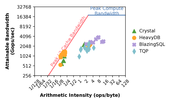
Figure 10. L2-Cache Roofline Model – for SSB queries (SF=16).

We present our profiling results in Figure 10. We discover that because Crystal and HeavyDB are very optimized, some queries have saturated the L2 cache bandwidth. In BlazingSQL and TQP, the query implementations are still far from the L2 cache bandwidth. In Figure 9, we saw that very few queries saturate the peak DRAM bandwidth. We observe that the AI of queries on the DRAM roofline model is lower than their corresponding AI on the L2 cache roofline model. This is reasonable especially in the case that queries have good utilization of the L2 cache bandwidth, because most memory requests complete at L2 cache level, so the GPU has less data to handle at the DRAM level. The second observation is that many of those queries have reached the peak L2 cache bandwidth. Queries with hash-join are more likely to saturate the L2 cache bandwidth. This is because SSB benchmark has relatively small hash tables that are likely to fit into the L2 cache of a high-end GPU (e.g., $40$ MB). Even though hash joins involve random accesses, queries may still exhibit good L2 cache utilization due to their small working sets. On the other hand, queries with simple filters are more likely to be bound by DRAM bandwidth: there is minimal data reuse, most data is streamed to the kernel, and cache utilization is generally lower.

✝ Finding. ❶ Queries with smaller working sets may be L2 cache bandwidth bound. ❷ Good L2 cache utilization leads to lower AI for DRAM.

6. MODEL-DRIVEN SCHEDULING

We have shown how to use the roofline model to identify resource bottlenecks for different queries in § 5. We now demonstrate how we can extend and apply the model to estimate the performance impact of changes in resource allocation and degree of concurrency.

6.1. Resource Allocation Mechanisms

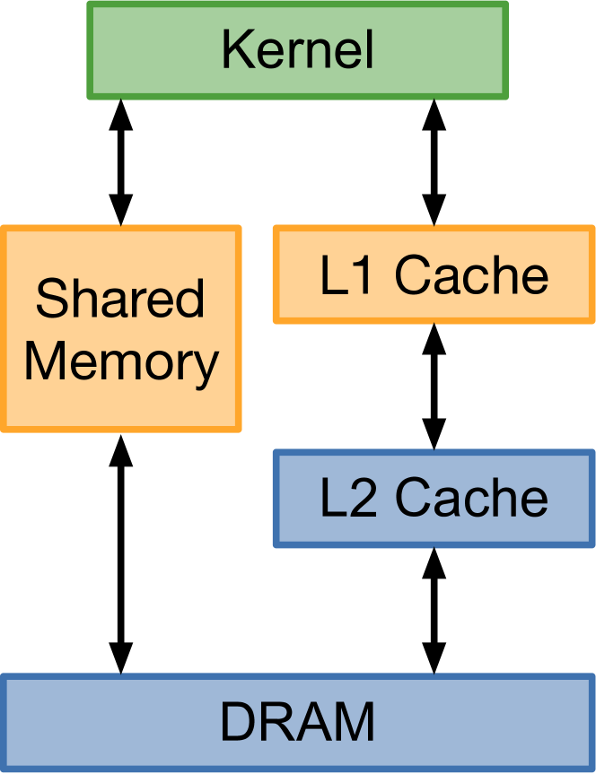
(a) GPU Memory hierarchy

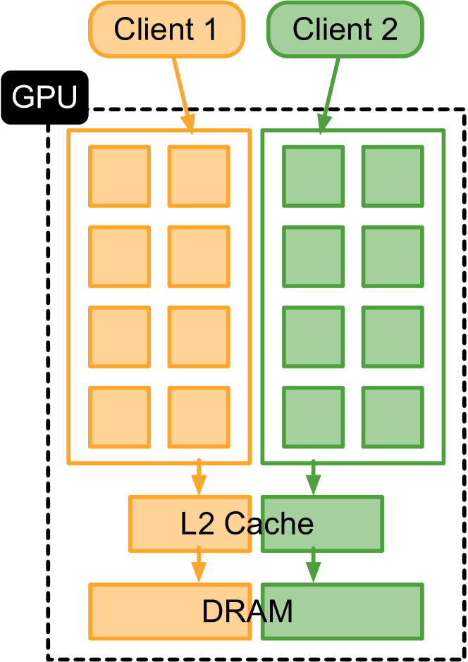
(b) MIG – resource partition example of multi-instance GPU (MIG).

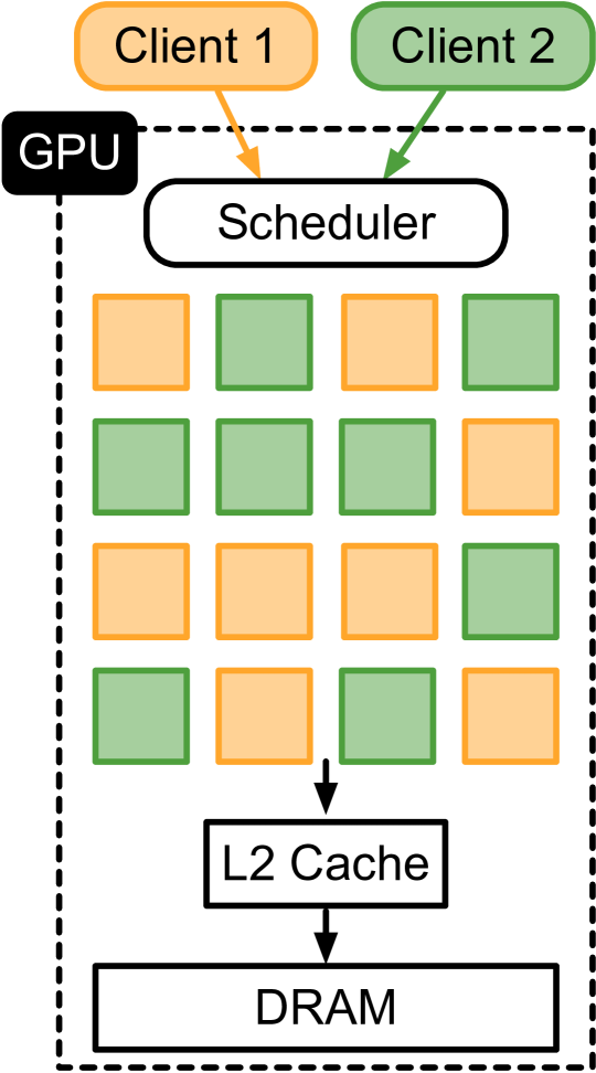
(c) MPS – resource partition example of multi-process service.

Figure 11. GPU Background and Concurrency Mechanisms – NVIDIA GPUs memory hierarchy, and supported concurrency mechanisms.

We first provide a brief overview about the memory hierarchy and currently supported mechanisms to perform resource allocation in NVIDIA GPUs. As Figure 11(a) shows, kernel execution can access data stored in either shared memory or L1 cache. Shared memory is managed completely by the user, but L1 cache is managed by the hardware. Each GPU SM has a private L1 cache and shared memory region, but the L2 cache and DRAM are shared across all GPU SMs. The memory hierarchy is consistent for all NVIDIA GPUs, but the specific values for capacity and bandwidth varies across GPUs. NVIDIA GPUs currently support two ways for allocating resources on the GPU, and providing concurrent GPU execution capability to processes: Multi-Instance GPU (MIG (NVIDIA, 2022b)) and Multi-Process Service (MPS (NVIDIA, 2021)). MIG is a new feature currently supported only on the A100, A30, and H100 GPUs (NVIDIA, 2022a).

MIG. MIG enables physical partitioning of GPU resources—SMs, L2 cache, DRAM capacity and bandwidth— which creates full isolation between concurrent processes. Figure 11(b) shows an example of resource allocation through MIG to support two concurrent clients with equal allocation ($\frac{1}{2}$ GPU resources) in this example. MIG also supports heterogeneous resource partitions to meet the different needs of different clients. MIG currently supports up to seven concurrent clients at its finest granularity: each partition gets about $\frac{1}{8}$ of compute and memory resources, while nearly $\frac{1}{8}$ of the resources is reserved for the MIG controller. MIG currently offers a total of $18$ choices for resource partitions on the A100.

MPS. MPS (NVIDIA, 2021) does logical resource partitioning to support concurrent execution. In old GPU generations, MPS only allows time-sharing of the GPU. Since Volta, MPS allows actual concurrent execution though lightweight resource partitioning by time-sharing SMs. In MPS, L2 cache and DRAM are still unified resources without any isolation. When MPS starts, it creates a scheduler on the GPU.

6.2. Model-Driven Resource Allocation

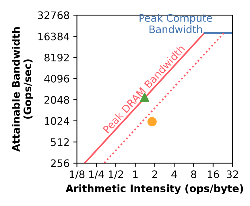
(a) Query performance, memory bandwidth, and compute bandwidth of full GPU resource (dashed line is projected memory bandwidth of half GPU resource).

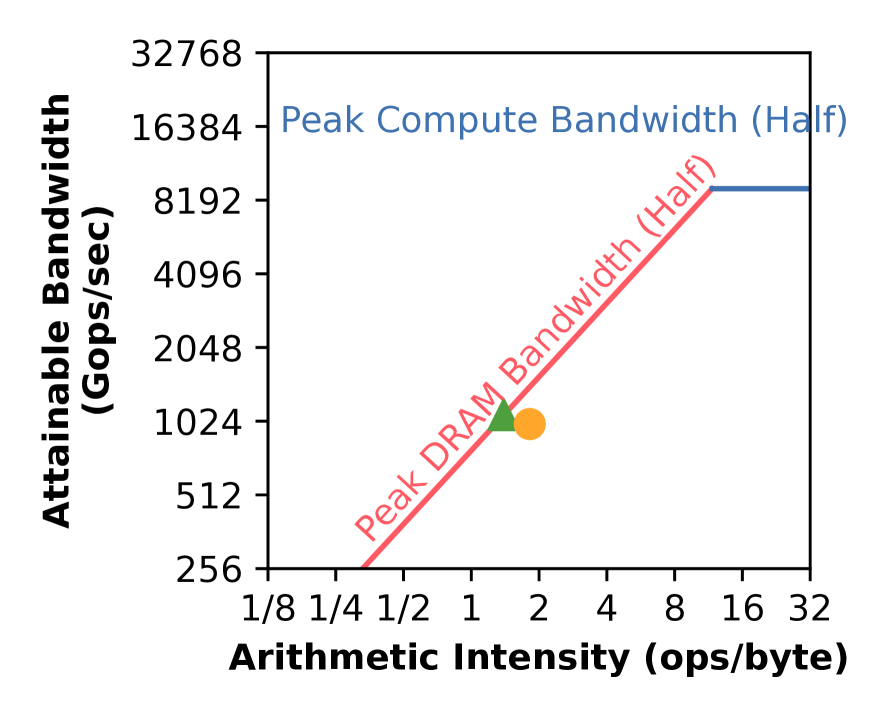
(b) Query performance, memory bandwidth, and compute bandwidth of half GPU resource.

Figure 12. Memory-Bound Queries – Performance impact on memory-bound queries (Q11 and Q31) for Crystal.

We now show how to use the roofline model to estimate performance impact for changes in resource allocation, which we can then use to select the optimal configuration. The model uses runtime statistical information which can be obtained from prior executions of recurring queries or by executing a representative workload.

We use DRAM as the target resource for illustration. Let $\mathrm{t}$ denote the query time under the current allocation and let $\mathrm{Bandwidth_{\scaleto{DRAM^{\prime}}{4pt}}}$ denote the new DRAM bandwidth. We predict the new query time $\mathrm{t}^{\prime}$ by using the following equation.

$$\mathrm{t}^{\prime} =\max\left(\mathrm{t}\text{, }\frac{\text{\# of Int. Ops}}{\mathrm{AI_{\scaleto{DRAM}{4pt}}}\times\mathrm{Bandwidth_{\scaleto{DRAM^{\prime}}{4pt}}}}\right)$$

This equation is proposed based on the observation that AI is determined by the implementation of the query and is unlikely to change when the resource allocation changes. Our model picks the maximum among the two terms in the equation—the first term for scenarios where bandwidth is not a bottleneck (and so, the time remains unchanged), and the second for scenarios where the change in memory bandwidth hurts performance. For the latter case, the denominator in the fraction is the maximum throughput at the given AI and allocated bandwidth. In this case, the query time is the time to execute the total integer operations at that throughput.  Figure 12 shows these two scenarios using representative queries (Q11, Q31) from Crystal, and full $\rightarrow$ half allocation change. Q31 under-utilizes the DRAM bandwidth and has no performance impact, whereas Q11 loses throughput (geometrically, the point shifts downwards) since it saturates the bandwidth. Finally, we compute $\mathrm{Slowdown_{\scaleto{DRAM}{4pt}}}={\mathrm{t}^{\prime}}/{\mathrm{t}}$.

L2 Bandwidth. As we discussed, the latest GPUs (NVIDIA, 2020) support both L2 and DRAM bandwidth partitioning. Similar to the above method, we can estimate the impact due to changed L2 allocation using the L2 roofline model. One challenge is how to combine both DRAM and L2 roofline models into a unified model to estimate the query slowdown. We solve this by simply using a max function to provide the total slowdown estimation as follows.

(3) $$\mathrm{Slowdown}=\max\left(\mathrm{Slowdown_{\scaleto{DRAM}{4pt}}},\mathrm{Slowdown_{\scaleto{L2Cache}{4pt}}}\right)$$

The rationale is that we empirically find that queries can be rarely bottlenecked by both memory resources (L2 and DRAM). For example, if a query has a very high utilization of the L2 cache bandwidth (i.e., it is bottlenecked by the L2), it only generates minimal traffic to DRAM, so it will not be affected by changes in DRAM bandwidth. Hence, one of the estimated slowdown terms is likely to be $1$ (no slowdown). Thus, we only need to use the $\max$ function to get the dominating slowdown value.

Compute-Bound.

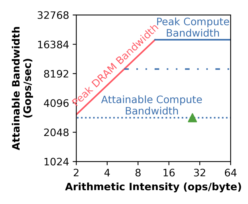
(a) Query performance, memory bandwidth, and compute bandwidth of full GPU resource (dashed-dotted line projects compute bandwidth of half GPU resource).

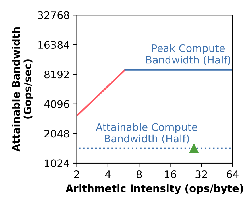
(b) Query performance, memory bandwidth, and compute bandwidth of half GPU resource.

Figure 13. Compute-Bound Queries – Performance impact on compute-bound queries (Q34 from BlazingSQL).

Last, we explain how we use the same model to estimate performance impact for compute-bound queries. In this case, because BlazingSQL has the most compute-bound implementations compared to the other systems, we pick BlazingSQL as the example to illustrate our idea.

Figure 13 left shows Q34 attainable bandwidth (i.e., throughput) and AI ($2886.74$ Gops/sec and $27.15$ ops/byte respectively). The peak compute bandwidth of the full GPU is $18247.00$ Gops/sec and that for half of GPU resources is near $9123.50$ Gops/sec (dashed and dotted line in Figure 13 left). It is clear that even the peak compute bandwidth for half GPU is beyond the attainable bandwidth of Q34, so the traditional roofline model would predict no performance slowdown. Nevertheless, we discover this is not the case as a result of the attainable compute bandwidth per SM being less than its peak due to execution inefficiencies (e.g., memory stalls). The overall compute bandwidth (attainable or peak) is the per-SM value $\times$ the number of SMs. When the GPU allocates less compute resources, it reduces the number of SMs allocated, but it cannot improve the execution efficiency (i.e., attainable compute bandwidth) of each SM. As a result, the overall attainable compute bandwidth will decrease (Figure 13 right). To estimate the resulting slowdown, we can simply use the ratio of resource allocations as follows.

(4) $$\mathrm{Slowdown_{\scaleto{Compute}{5pt}}}=\frac{1}{\mathrm{ComputeAllocationRatio}}$$

For example, if the GPU compute resources are halved, then the attainable bandwidth can be calculated as half of the original attainable bandwidth with full GPU resources.

Unified Model. Now that we have proposed two models for estimating slowdowns with changing allocations—one for memory resources and one for compute resources, the last step is to determine which model to use. We use a simple heuristic, which is commonly used (Mao, 2021; Ofenbeck et al., 2014), to determine whether an application is compute or memory-bound. As shown below, we can determine if an application tends to be compute-bound based on the AI and peak compute and DRAM bandwidths of the GPU. The final $\mathrm{Slowdown}$

$$=\begin{cases}\text{(4)},\text{if }\mathrm{AI_{\scaleto{DRAM}{4pt}}}>\frac{\mathrm{Bandwidth_{\scaleto{Compute}{5pt}}}}{\mathrm{Bandwidth_{\scaleto{DRAM}{4pt}}}}\text{or }\mathrm{AI_{\scaleto{L2Cache}{4pt}}}>\frac{\mathrm{Bandwidth_{\scaleto{Compute}{5pt}}}}{\mathrm{Bandwidth_{\scaleto{L2Cache}{4pt}}}}\\ \text{(3)},\text{otherwise}\end{cases}$$

If the application is more compute-bound, then we use the model to account for compute bandwidth reduction. Otherwise, we apply the model for DRAM or L2 cache bandwidth reduction.

The limitation of this approach is that it can be more easily used to estimate performance impact of downsizing both memory and compute resources. Additionally, it can be also used to reason about performance impact of upsizing compute resource. However, it could have inaccurate estimation for performance impact of upsizing memory resources when they are no longer a bottleneck.

6.3. Model-Driven Concurrent Scheduling

Next, we extend the model to estimate end-to-end performance impact for different degrees of concurrency. This can be used to determine the optimal concurrency for the best performance.

CPU and Constant Overhead. To construct the model, we first need to consider additional overheads for query executions. For CPU overheads, our model includes the overhead of query optimization and compilation. For some systems (e.g., HeavyDB, BlazingSQL), even though the same query has already been optimized and compiled to a binary, each query invocation still introduces some constant overhead on the CPU side. For all systems, we also consider those overheads. We will later show insights about how concurrency is also beneficial to alleviate those overheads. There are two additional major overheads that we consider— GPU setup overhead, which includes GPU context initialization and memory allocations, and data transfer overhead. All systems cache tables on the GPU device for future query executions, so the data transfer overhead is also only a one time cost.

End-to-End Performance. We now can estimate the end-to-end query execution time individually for each process. When the system varies the resources, the model will adjust the query GPU execution time. Other overheads will remain unchanged. Now to consider time from multiple concurrent processes $P$, we use a $\max$ function because the longest running process will determine the end-to-end query execution time for concurrent executions.

$$\mathrm{ExecTime}=\max\left(\mathrm{ExecTime_{\scaleto{P_{1}}{4pt}}},\mathrm{ExecTime_{\scaleto{P_{2}}{4pt}}}\text{ ... }\mathrm{ExecTime_{\scaleto{P_{n}}{4pt}}}\right)$$

Our model can also be used to estimate query performance vs. degree of concurrency for MPS (§ 6.1) excluding accounting for interference in accesses to the shared L2 cache and DRAM.

6.4. Evaluation

We focus on answering the following questions:

• RQ1 – How accurate is our model for estimating GPU query execution performance vs. resource allocation compared to a naive linear scaling model?

• RQ2 – How beneficial is concurrent query execution?

• RQ3 – How good is our model to estimate end-to-end query execution performance vs. degree of concurrency?

We demonstrate our approach using HeavyDB for illustration, but expect similar conclusions to hold for other systems as well.

RQ1 – Model Accuracy on Resource Allocation.

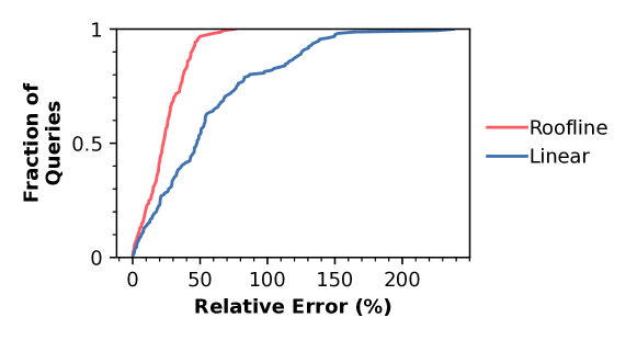
Figure 14. Query Time Estimation Error – Comparison of CDF of query time estimation error between roofline and linear model.

Figure 14 shows the distribution (CDF) of relative error, which is computed as $\left(\frac{|\text{Estimate Time}-\text{Actual Time}|}{\text{Actual Time}}\right)\times 100$, for all SSB queries with four SFs ($2,4,8,16$) running on HeavyDB, using estimates from our roofline model and from a linear scaling model ($\mathrm{t}^{\prime}=\frac{\mathrm{t}}{\mathrm{ComputeAllocationRatio}}$) that we use as a baseline. Both models use profiled information from a single run of each query with a given SF and with full GPU allocation to estimate query runtimes at other allocations. We observe that our roofline model is substantially more accurate than the baseline—the median and 95^th percentile errors are $22.73$% and $47.79$% respectively in contrast to $48.39$% and $139.77$% for the baseline. Queries run with large SFs or having mainly sequential scan operations are more likely to have linear scaling with resource allocation changes. However, our roofline model provides better estimation accuracy for queries whose performance do not scale linearly with GPU resources (§ 1).

RQ2 – Benefit of Concurrent Query Execution. We implemented a concurrent query execution system and designed the following experiment to evaluate benefits with Degree of Concurrency (DoC) = $2$, $3$, and $7$, over DoC=$1$ (no concurrency), for SSB queries on HeavyDB. We configured the GPU, through MIG, to support the required DoC, and started the corresponding number of HeavyDB instances, one on each GPU partition. We construct a simple scheduler to dispatch SSB queries in a randomized sequence to each HeavyDB instance, repeated $1000$ times. We then measure the overall throughput (queries per second i.e., QPS) for the GPU.

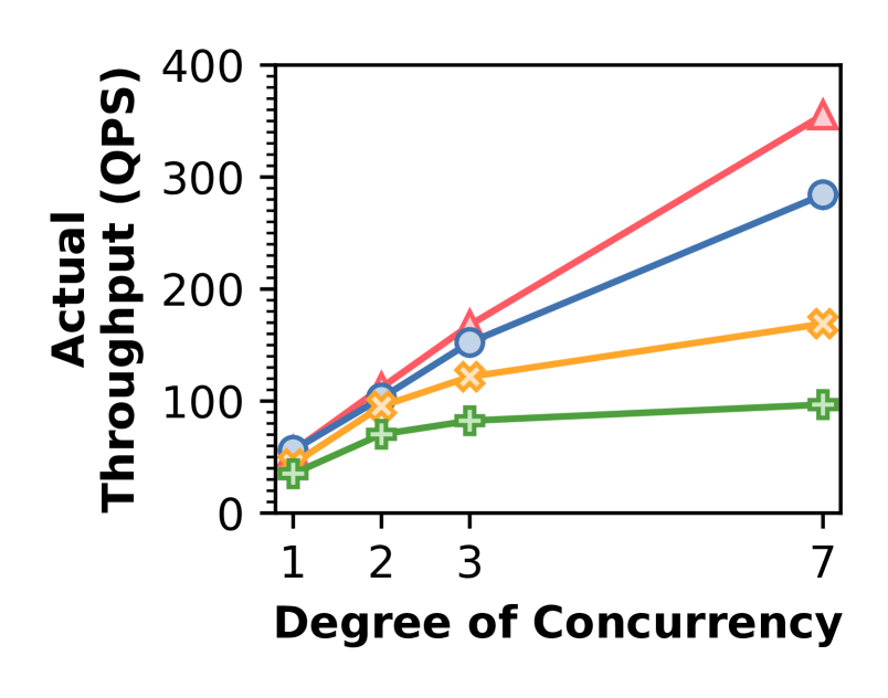
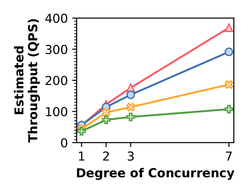
Figure 15. Throughput vs. Degree of Concurrency – Comparison between actual and estimated throughput of running queries concurrently.

Figure 15 (left) shows the actual (measured) throughput for different DoC. We find that concurrent execution provides near-linear performance improvement—$6.43\times$ and $5.06\times$ for SF=$2$ and SF=$4$ respectively at DoC=$7$ (over DoC=$1$). Queries at small SFs typically do not fully saturate any resource. More queries can finish within a fixed time with concurrent execution, so the overall throughput increases. In contrast, queries are more easily affected by resource reduction at larger SFs, leading to a significant increase in query latency that overshadows the gains of concurrent execution. However, concurrency is still able to hide CPU latency overhead (§ 4.2), leading to substantial throughput improvements—$3.85\times$ and $2.75\times$ for SF=$8$ and SF=$16$ respectively at DoC=$7$ (over DoC=$1$).

RQ3 – Model Accuracy on Degree of Concurrency. Figure 15 (right) shows the estimated overall throughput vs DoC for the above experimental setting. We use our models to estimate end-to-end query execution time for all DoC using profiling data from a single run of the query with full GPU allocation (DoC=$1$). Our estimated throughputs are very close to actuals, both for absolute values as well as for scaling trends (linear and non-linear).

7. RELATED WORK

GPU database systems. Suh et al. (Suh et al., 2022) is the most recent study to compare different GPU database systems. It only focuses on end-to-end execution time comparison of different systems on different GPUs. However, our paper shares more insights on internals of GPU execution efficiency. Yin and Yang (Yuan et al., 2013) studies GPU execution of SSB (Rabl et al., 2013), which focuses on presenting time breakdown between kernels and data transfers, but it never examines the effciency of each kernel. Pump up the Volume (Lutz et al., 2020) and triton join (Lutz et al., 2022) study performance impact from newer CPU-GPU interconnects on out-of-GPU hash-join. GPL (Paul et al., 2016) also observes that the resource of GPU can be underutilized during query execution. Furst et al. (Furst et al., 2017) studies GPU kernel efficiency but only focuses on showing GPU occupancy vs. types of instruction comparison. Funke et al. (Funke et al., 2018; Funke and Teubner, 2020) and Paul et al. (Paul et al., 2020) optimize JIT compilers for better GPU execution efficiency through kernel fusions and thread divergence elimination. Sioulas et al. (Sioulas et al., 2019) implements partitioned hash-join in GPU. Shanbhag et al. (Shanbhag et al., 2022) also extends Crystal library for in-GPU compression. Instead, HippogriffDB (Li et al., 2016) accelerate query performance by supporting GPU execution directly on compressed data. Mordred (Yogatama et al., 2022) and HetExchange (Chrysogelos et al., 2019) both explore CPU-GPU query executions. Rosenfeld et al. (Rosenfeld et al., 2023) provides an in-depth overview of CPU-GPU database systems. Gacco (Boeschen and Binnig, 2022) instead studies transactional query processing on GPUs. MGJoin (Paul et al., 2021) and Maltenberger et al. (Maltenberger et al., 2022) evaluates join and sorting algorithms for multi-GPU systems. Doraiswamy and Freire (Doraiswamy and Freire, 2020) propose to use GPUs to process spatial data (e.g., geometric objects) in database systems. We cover existing GPU database systems in § 2. Our work provides in-depth micro-architectural analysis of existing systems.

GPU performance modeling. Hong and Kim (Hong and Kim, 2009) model performance of early generation GPUs, where GPU caches are still not mature, so the focus is on GPU DRAM and compute bandwidths. Zhang et al. (Zhang and Owens, 2011) provides performance optimization suggestions to developers through GPU performance modeling with micro-benchmarking profiling. Wu et al. (Wu et al., 2015) instead proposes to use machine learning approach to predict kernel performance, which also requires profiling performance counters on real hardware. Baghsorkhi et al. (Baghsorkhi et al., 2010) uses code analysis to consider performance impact from control flow divergence and memory bank conflicts. Our approach of using the roofline models provides a simple way to analyze performance impact for different GPU resources without requiring code analysis or machine learning models.

Gables (Hill and Janapa Reddi, 2019) uses roofline models to study SoC platforms with multiple accelerators. Ding et al. (Ding and Williams, 2019) and Lopes et al. (Lopes et al., 2017) also apply roofline models to GPUs. Ding et al. captures all instruction for AI, which can lead to inaccurate estimations. Lopes et al. also explores the cache-aware aspect, but does not differentiate between AI at cache-level and at DRAM-level, in contrast to our work. Additionally, we extend and apply the roofline model to estimate query performance for different resource allocations on the GPU, that has not been explored in prior work.

Concurrent execution in GPUs. Yu et al. (Yu et al., 2022) has also surveyed the tradeoff between MIG and MPS. The paper shares the potential opportunities and use cases of using concurrent execution in GPUs. Tan et al. (Tan et al., 2021) explores accelerating deep neural network (DNN) inference by using MIG. Kass et al. (Kaas et al., 2022) instead investigates DNN training in MIG. MISO (Li et al., 2022) uses MPS to find the best GPU partition configuration and run the actual execution in MIG to achieve the best performance. In our work, we support relational query operations in the form of concurrent execution, which is often limited by the GPU memory resource. Instead, DNN inference is more compute-bound. Our work uses simple models to estimate performance with different GPU resource limits, whereas others (Tan et al., 2021) require profiling the execution for different configurations.

8. RESEARCH DIRECTIONS

We conclude with a discussion about directions for research in hardware and software improvements for GPU database systems.

GPU L2 Cache Improvements. The GPU L2 cache can commonly be a bottlenecked resource (§ 5.2). Current GPUs adopt a shared L2 cache design, in which data in GPU DRAM is mapped to different L2 cache slices based on their address in memory. GPU SMs that access near-memory addresses frequently (e.g., for probing a relatively small hash-table) need to serialize memory accesses in the L2 cache, because the requested cachelines are all located in the same cache slice. Previous works (Zhao et al., 2019) have shown that new GPU architectures with a private L2 cache for a cluster of SMs can provide better bandwidth. Database developers can store frequently-accessed data in different memory partitions (consequently, mapped to different L2 cache slices) to maximize L2 cache utilization.

Efficient and Automatic Kernel Fusion. We observed that kernel fusion is one of the most important techniques for achieving good performance by avoiding unnecessary data materialization (§ 4.6). Nevertheless, only HeavyDB supports automatic kernel fusion, but the compilation overhead is not negligible (Figure 2). TQP leverages PyTorch for operator fusion, but the set of kernels that can be automatically fused is minimal, and mostly ML-related (e.g., convolutions with activation functions) (Chen et al., 2018; Jia et al., 2019). On the CPU side, in the last few years several techniques have been proposed for efficient operator fusion (Neumann, 2021). Applying the same techniques in the GPU space is an interesting research direction.

Flexible Resource Allocation. MIG currently does not allow separately selecting compute and memory resource allocations, and only a set of predefined resource partitions are available to choose from. However, results in § 5.2 show that queries have diverse resource requirements. Decoupled partitioning of GPU resources can create more optimization opportunities for database workloads.

GPU Resource-Aware QO. As we discussed earlier (§ 1), there is a wide variety of GPUs available today having many different sizes for various resources. Additionally, MIG capability has increased the set of possible resource allocations to run a query. Having a resource-aware query optimizer, for GPU databases, that adapts query plans to allocated resources may improve query performance compared to that with a fixed, resource-oblivious query plan.

❶ Example: Memory Coalescing. We observed that most queries have long memory stalls (§ 4.5). One way to reduce memory stalls is to increase memory coalescing (Harris, 2013). For example, WarpDrive (Jünger et al., 2018) demonstrates that achieving better memory coalescing for accesses to GPU DRAM can improve performance even though it incurs more arithmetic operations. Nevertheless, for newer GPUs with larger L2 cache size (less than $10$ MB for previous generation GPUs (TechPowerUp, 2022a, b)), this optimization may no longer be critical, if a hash-table fits into the L2 cache. Instead, additional arithmetic operations caused by memory coalescing can hurt performance.

❷ Example: Exploiting L1 Cache. GPUs offer developers capability to control data caching behavior (e.g., bypass L1 cache or not and cache replacement policy) through PTX (NVIDIA, 2022d). Previously, the per-SM L1 cache in old generation GPUs had longer latency and lower capacity (e.g., $24$ KB in P100 (TechPowerUp, 2022a) in contrast to $192$ KB in A100), so it was skipped as optimization to reduce memory access latency for workloads with many random accesses (e.g., hash-join). However, using the L1 cache in newer GPUs can be very beneficial, especially for skewed workloads, because data reuse is higher.

Supporting Larger Datasets. While GPU memory capacities have increased, the largest size at the time of this writing is possibly 128 GB (AMD, 2021) which is several times smaller than CPU memory in high-end servers. Our experiments also show diminishing reductions in data movement overhead for higher PCIe generations (§ 4.1). Considering these factors, it would be useful to explore how GPU database systems could efficiently process larger datasets, e.g., by using techniques such as query processing on compressed data (Li et al., 2016).

Time Prediction for different GPUs. We have demonstrated (§ 6.4) that our models produce good estimates of query performance for different resource limits on the same GPU architecture. Future research can explore extending this capability to predict performance for different GPU architectures as well.

9. CONCLUSIONS

In this work, we provide micro-architectural insights studied on existing GPU database systems. We demonstrate two models to do query performance analysis. Our proposed approach shows good accuracy at estimating query performance with respect to different GPU resources and concurrency.

References

- (1)
- pci (2017) 2017. PCIe 4.0 specification finally out with 16 GT/s on tap. [Online] Available from: https://techreport.com/news/32064/pcie-4-0-specification-finally-out-with-16-gts-on-tap/.
- pci (2019) 2019. PCI-SIG Achieves 32GT/s with New PCI Express 5.0 Specification. [Online] Available from: https://www.businesswire.com/news/home/20190529005766/en/PCI-SIG%C2%AE-Achieves-32GTs-with-New-PCI-Express%C2%AE-5.0-Specification.
- jia (2021) 2021. Dissecting the Ampere GPU Architecture through Microbenchmarking. [Online] Available from: https://www.nvidia.com/en-us/on-demand/session/gtcspring21-s33322/.
- pci (2022a) 2022a. PCI-SIG Announces PCI Express 7.0 Specification to Reach 128 GT/s. [Online] Available from: https://www.businesswire.com/news/home/20220621005137/en.
- pci (2022b) 2022b. PCI-SIG Releases PCIe 6.0 Specification Delivering Record Performance to Power Big Data Applications. [Online] Available from: https://www.businesswire.com/news/home/20220111005011/en/PCI-SIG%C2%AE-Releases-PCIe%C2%AE-6.0-Specification-Delivering-Record-Performance-to-Power-Big-Data-Applications.
- Ailamaki et al. (1999) Anastassia Ailamaki, David J DeWitt, Mark D Hill, and David A Wood. 1999. DBMSs On A Modern Processor: Where Does Time Go? PVLDB (1999).
- AMD (2021) AMD. 2021. AMD Instinct MI250 Accelerator. [Online] Available from: https://www.amd.com/system/files/documents/amd-instinct-mi200-datasheet.pdf.
- Armbrust et al. (2015) Michael Armbrust, Reynold S. Xin, Cheng Lian, Yin Huai, Davies Liu, Joseph K. Bradley, Xiangrui Meng, Tomer Kaftan, Michael J. Franklin, Ali Ghodsi, and Matei Zaharia. 2015. Spark SQL: Relational Data Processing in Spark. In SIGMOD. 1383–1394.
- Baghsorkhi et al. (2010) Sara S Baghsorkhi, Matthieu Delahaye, Sanjay J Patel, William D Gropp, and Wen-mei W Hwu. 2010. An Adaptive Performance Modeling Tool for GPU Architectures. In PPoPP. 10.
- Bakkum and Chakradhar (2010) Peter Bakkum and Srimat Chakradhar. 2010. Efficient Data Management for GPU Databases. https://github.com/bakks/virginian/.
- BlazingSQL (2021) BlazingSQL. 2021. BlazingSQL. https://github.com/BlazingDB/blazingsql.
- Boeschen and Binnig (2022) Nils Boeschen and Carsten Binnig. 2022. GaccO - A GPU-accelerated OLTP DBMS. In SIGMOD. 1003–1016.
- Chen et al. (2018) Tianqi Chen, Thierry Moreau, Ziheng Jiang, Lianmin Zheng, Eddie Yan, Meghan Cowan, Haichen Shen, Leyuan Wang, Yuwei Hu, Luis Ceze, Carlos Guestrin, and Arvind Krishnamurthy. 2018. TVM: An Automated End-to-end Optimizing Compiler for Deep Learning. In Proceedings of the 12th USENIX Conference on Operating Systems Design and Implementation.
- Chrysogelos et al. (2019) Periklis Chrysogelos, Manos Karpathiotakis, Raja Appuswamy, and Anastasia Ailamaki. 2019. HetExchange: Encapsulating Heterogeneous CPU-GPU Parallelism in JIT Compiled Engines. PVLDB (2019), 544–556.
- Ding and Williams (2019) Nan Ding and Samuel Williams. 2019. An Instruction Roofline Model for GPUs. In PBMS. 7–18.
- Doraiswamy and Freire (2020) Harish Doraiswamy and Juliana Freire. 2020. A GPU-friendly Geometric Data Model and Algebra for Spatial Queries. In SIGMOD. 1875–1885.
- Floratos et al. (2021) Sofoklis Floratos, Mengbai Xiao, Hao Wang, Chengxin Guo, Yuan Yuan, Rubao Lee, and Xiaodong Zhang. 2021. NestGPU: Nested Query Processing on GPU. In ICDE. 1008–1019.
- Funke et al. (2018) Henning Funke, Sebastian Breß, Stefan Noll, Volker Markl, and Jens Teubner. 2018. Pipelined Query Processing in Coprocessor Environments. In SIGMOD. 1603–1618.
- Funke and Teubner (2020) Henning Funke and Jens Teubner. 2020. Data-Parallel Query Processing on Non-Uniform Data. PVLDB (2020), 884–897.
- Furst et al. (2017) Emily Furst, Mark Oskin, and Bill Howe. 2017. Profiling a GPU database implementation: a holistic view of GPU resource utilization on TPC-H queries. In DaMON. 1–6.
- Harris (2013) Mark Harris. 2013. How to Access Global Memory Efficiently in CUDA C/C++ Kernels. [Online] Availble from: https://developer.nvidia.com/blog/how-access-global-memory-efficiently-cuda-c-kernels/.
- He et al. (2022) Dong He, Supun Nakandala, Dalitso Banda, Rathijit Sen, Karla Saur, Kwanghyun Park, Carlo Curino, Jesús Camacho-Rodríguez, Konstantinos Karanasos, and Matteo Interlandi. 2022. Query Processing on Tensor Computation Runtimes.
- HeavyDB (2022) HeavyDB. 2022. HeavyDB. https://github.com/heavyai/heavydb.
- Heimel et al. (2013) Max Heimel, Michael Saecker, Holger Pirk, Stefan Manegold, and Volker Markl. 2013. Hardware-Oblivious Parallelism for in-Memory Column-Stores. PVLDB (2013), 709–720.
- Hill and Janapa Reddi (2019) Mark Hill and Vijay Janapa Reddi. 2019. Gables: A Roofline Model for Mobile SoCs. In HPCA. 317–330.
- Hong and Kim (2009) Sunpyo Hong and Hyesoon Kim. 2009. An Analytical Model for a GPU Architecture with Memory-Level and Thread-Level Parallelism Awareness. In ISCA. 12.
- Ilic et al. (2014) Aleksandar Ilic, Frederico Pratas, and Leonel Sousa. 2014. Cache-Aware Roofline Model: Upgrading the Loft. IEEE CAL (2014), 21–24.
- Jia et al. (2019) Zhihao Jia, Oded Padon, James Thomas, Todd Warszawski, Matei Zaharia, and Alex Aiken. 2019. TASO: Optimizing Deep Learning Computation with Automatic Generation of Graph Substitutions. In Proceedings of the 27th ACM Symposium on Operating Systems Principles. ACM, New York, NY, USA, 47–62.
- Jünger et al. (2018) D. Jünger, C. Hundt, and B. Schmidt. 2018. WarpDrive: Massively Parallel Hashing on Multi-GPU Nodes. In IPDPS. 441–450.
- Jyothi et al. (2016) Sangeetha Abdu Jyothi, Carlo Curino, Ishai Menache, Shravan Matthur Narayanamurthy, Alexey Tumanov, Jonathan Yaniv, Ruslan Mavlyutov, Inigo Goiri, Subru Krishnan, Janardhan Kulkarni, et al. 2016. Morpheus: Towards Automated SLO for Enterprise Clusters. In OSDI. 117–134.
- Kaas et al. (2022) Anders Friis Kaas, Stilyan Petrov Paleykov, Ties Robroek, and Pınar Tözün. 2022. Deep Learning Training on Multi-Instance GPUs.
- Kohei (2022) KaiGai Kohei. 2022. PG-Strom. https://github.com/heterodb/pg-strom.
- Krolik et al. (2021) Alexander Krolik, Clark Verbrugge, and Laurie Hendren. 2021. R3d3: Optimized Query Compilation on GPUs. In CGO. 277–288.
- Lattner and Adve (2004) Chris Lattner and Vikram Adve. 2004. LLVM: A Compilation Framework for Lifelong Program Analysis and Transformation. In CGO. 75–88.
- Li et al. (2022) Baolin Li, Tirthak Patel, Siddarth Samsi, Vijay Gadepally, and Devesh Tiwari. 2022. MISO: Exploiting Multi-Instance GPU Capability on Multi-Tenant Systems for Machine Learning. In SoCC. 173–189.
- Li et al. (2016) Jing Li, Hung-Wei Tseng, Chunbin Lin, Yannis Papakonstantinou, and Steven Swanson. 2016. HippogriffDB: Balancing I/O and GPU Bandwidth in Big Data Analytics. PVLDB (2016), 1647–1658.
- Lopes et al. (2017) André Lopes, Frederico Pratas, Leonel Sousa, and Aleksandar Ilic. 2017. Exploring GPU Performance, Power and Energy-Efficiency Bounds with Cache-aware Roofline Modeling. In ISPASS. 259–268.
- Lutz et al. (2020) Clemens Lutz, Sebastian Breß, Steffen Zeuch, Tilmann Rabl, and Volker Markl. 2020. Pump Up the Volume: Processing Large Data on GPUs with Fast Interconnects. In SIGMOD. 1633–1649.
- Lutz et al. (2022) Clemens Lutz, Sebastian Breß, Steffen Zeuch, Tilmann Rabl, and Volker Markl. 2022. Triton Join: Efficiently Scaling to a Large Join State on GPUs with Fast Interconnects. In SIGMOD. 1017–1032.
- Maltenberger et al. (2022) Tobias Maltenberger, Ivan Ilic, Ilin Tolovski, and Tilmann Rabl. 2022. Evaluating Multi-GPU Sorting with Modern Interconnects. In SIGMOD. 1795–1809.
- Mao (2021) Lei Mao. 2021. Math-Bound VS Memory-Bound Operations. https://leimao.github.io/blog/Math-Bound-VS-Memory-Bound-Operations/.
- Neumann (2011) Thomas Neumann. 2011. Efficiently Compiling Efficient Query Plans for Modern Hardware. PVLDB (2011), 539–550.
- Neumann (2021) Thomas Neumann. 2021. Evolution of a Compiling Query Engine. Proc. VLDB Endow. 14, 12 (jul 2021), 3207–3210. https://doi.org/10.14778/3476311.3476410
- NVIDIA (2016) NVIDIA. 2016. nvidia-smi Documentation. [Online] Available from: https://developer.download.nvidia.com/compute/DCGM/docs/nvidia-smi-367.38.pdf.
- NVIDIA (2020) NVIDIA. 2020. NVIDIA A100 TENSOR CORE GPU Unprecedented Acceleration at Every Scale. [Online] Available from: https://www.nvidia.com/content/dam/en-zz/Solutions/Data-Center/a100/pdf/nvidia-a100-datasheet-nvidia-us-2188504-web.pdf.
- NVIDIA (2021) NVIDIA. 2021. NVIDIA Multi-Process Service Introduction. [Online] Available from: https://docs.nvidia.com/deploy/mps/index.html.
- NVIDIA (2022a) NVIDIA. 2022a. NVIDIA Multi-Instance GPU. [Online] Available from: https://www.nvidia.com/en-us/technologies/multi-instance-gpu/.
- NVIDIA (2022b) NVIDIA. 2022b. NVIDIA Multi-Instance GPU User Guide. [Online] Available from: https://docs.nvidia.com/datacenter/tesla/mig-user-guide/.
- NVIDIA (2022c) NVIDIA. 2022c. NVIDIA NSight Systems User Guide. [Online] Available from: https://docs.nvidia.com/nsight-systems/UserGuide/index.html.
- NVIDIA (2022d) NVIDIA. 2022d. Parallel Thread Execution ISA Version 7.8. [Online] Available from: https://docs.nvidia.com/cuda/parallel-thread-execution/index.html.
- NVIDIA (2022e) NVIDIA. 2022e. Thrust. [Online] Availble from: https://docs.nvidia.com/cuda/thrust/index.html.
- Ofenbeck et al. (2014) Georg Ofenbeck, Ruedi Steinmann, Victoria Caparros, Daniele G. Spampinato, and Markus Püschel. 2014. Applying the Roofline Model. In ISPASS. 76–85.
- O’Neil et al. (2009) Patrick O’Neil, Elizabeth O’Neil, Xuedong Chen, and Stephen Revilak. 2009. The Star Schema Benchmark and Augmented Fact Table Indexing. Springer-Verlag, Berlin, Heidelberg, 237–252. https://doi.org/10.1007/978-3-642-10424-4_17
- Paszke et al. (2019) Adam Paszke, Sam Gross, Francisco Massa, Adam Lerer, James Bradbury, Gregory Chanan, Trevor Killeen, Zeming Lin, Natalia Gimelshein, Luca Antiga, Alban Desmaison, Andreas Kopf, Edward Yang, Zachary DeVito, Martin Raison, Alykhan Tejani, Sasank Chilamkurthy, Benoit Steiner, Lu Fang, Junjie Bai, and Soumith Chintala. 2019. PyTorch: An Imperative Style, High-Performance Deep Learning Library. In NeurIPS. 8024–8035.
- Paul et al. (2020) Johns Paul, Bingsheng He, Shengliang Lu, and Chiew Tong Lau. 2020. Improving Execution Efficiency of Just-in-Time Compilation Based Query Processing on GPUs. PVLDB (2020), 202–214.
- Paul et al. (2016) Johns Paul, Jiong He, and Bingsheng He. 2016. GPL: A GPU-based Pipelined Query Processing Engine. In SIGMOD. 1935–1950.
- Paul et al. (2021) Johns Paul, Shengliang Lu, Bingsheng He, and Chiew Tong Lau. 2021. MG-Join: A Scalable Join for Massively Parallel Multi-GPU Architectures. In SIGMOD. 1413–1425.
- Rabl et al. (2013) Tilmann Rabl, Meikel Poess, Hans-Arno Jacobsen, Patrick O’Neil, and Elizabeth O’Neil. 2013. Variations of the Star Schema Benchmark to Test the Effects of Data Skew on Query Performance. In ICPE. 361.
- Rosenfeld et al. (2023) Viktor Rosenfeld, Sebastian Breß, and Volker Markl. 2023. Query Processing on Heterogeneous CPU/GPU Systems. Comput. Surveys (2023), 1–38.
- Sen et al. (2020) Rathijit Sen, Alekh Jindal, Hiren Patel, and Shi Qiao. 2020. Autotoken: Predicting peak parallelism for big data analytics at microsoft. PVLDB (2020), 3326–3339.
- Sen and Ramachandra (2018) Rathijit Sen and Karthik Ramachandra. 2018. Characterizing resource sensitivity of database workloads. In HPCA. 657–669.
- Shanbhag (2020) Anil Shanbhag. 2020. Crystal GPU Library. https://github.com/anilshanbhag/crystal.
- Shanbhag et al. (2020) Anil Shanbhag, Samuel Madden, and Xiangyao Yu. 2020. A Study of the Fundamental Performance Characteristics of GPUs and CPUs for Database Analytics. In SIGMOD. 1617–1632.
- Shanbhag et al. (2022) Anil Shanbhag, Bobbi W. Yogatama, Xiangyao Yu, and Samuel Madden. 2022. Tile-Based Lightweight Integer Compression in GPU. In SIGMOD. 1390–1403.
- Shen et al. (2019) Jian Shen, Ze Wang, David Wang, Jeremy Shi, and Steven Chen. 2019. AresDB. https://github.com/uber/aresdb.
- Sioulas et al. (2019) P. Sioulas, P. Chrysogelos, M. Karpathiotakis, R. Appuswamy, and A. Ailamaki. 2019. Hardware-Conscious Hash-Joins on GPUs. In ICDE. 698–709.
- Sirin and Ailamaki (2020) Utku Sirin and Anastasia Ailamaki. 2020. Micro-Architectural Analysis of OLAP: Limitations and Opportunities. PVLDB (2020), 840–853.
- Suh et al. (2022) Young-Kyoon Suh, Junyoung An, Byungchul Tak, and Gap-Joo Na. 2022. A Comprehensive Empirical Study of Query Performance Across GPU DBMSes. SIGMETRICS (2022), 1–29.
- Tan et al. (2021) Cheng Tan, Zhichao Li, Jian Zhang, Yu Cao, Sikai Qi, Zherui Liu, Yibo Zhu, and Chuanxiong Guo. 2021. Serving DNN Models with Multi-Instance GPUs: A Case of the Reconfigurable Machine Scheduling Problem.
- Team (2018) RAPIDS Development Team. 2018. RAPIDS: Collection of Libraries for End to End GPU Data Science. https://rapids.ai
- TechPowerUp (2022a) TechPowerUp. 2022a. NVIDIA Tesla P100 PCIe 16 GB. [Online] Available from: https://www.techpowerup.com/gpu-specs/tesla-p100-pcie-16-gb.c2888.
- TechPowerUp (2022b) TechPowerUp. 2022b. NVIDIA Tesla V100 PCIe 32 GB. [Online] Available from: https://www.techpowerup.com/gpu-specs/tesla-v100-pcie-32-gb.c3184.
- Williams et al. (2009) Samuel Williams, Andrew Waterman, and David Patterson. 2009. Roofline: An Insightful Visual Performance Model for Floating-Point Programs and Multicore Architectures. Technical Report. 10 pages.
- Wu et al. (2015) Gene Wu, Joseph L. Greathouse, Alexander Lyashevsky, Nuwan Jayasena, and Derek Chiou. 2015. GPGPU Performance and Power Estimation Using Machine Learning. In HPCA. 564–576.
- Wu et al. (2014) Haicheng Wu, Gregory Diamos, Tim Sheard, Molham Aref, Sean Baxter, Michael Garland, and Sudhakar Yalamanchili. 2014. Red Fox: An Execution Environment for Relational Query Processing on GPUs. In CGO. 44–54.
- Yogatama et al. (2022) Bobbi W. Yogatama, Weiwei Gong, and Xiangyao Yu. 2022. Orchestrating Data Placement and Query Execution in Heterogeneous CPU-GPU DBMS. PVLDB (2022), 2491–2503.
- Yu et al. (2022) Fuxun Yu, Di Wang, Longfei Shangguan, Minjia Zhang, Chenchen Liu, and Xiang Chen. 2022. A Survey of Multi-Tenant Deep Learning Inference on GPU.
- Yuan et al. (2013) Yuan Yuan, Rubao Lee, and Xiaodong Zhang. 2013. The Yin and Yang of Processing Data Warehousing Queries on GPU Devices. PVLDB (2013), 817–828.
- Zhang and Owens (2011) Yao Zhang and John D. Owens. 2011. A Quantitative Performance Analysis Model for GPU Architectures. In HCPA. 382–393.
- Zhao et al. (2019) Xia Zhao, Almutaz Adileh, Zhibin Yu, Zhiying Wang, Aamer Jaleel, and Lieven Eeckhout. 2019. Adaptive Memory-Side Last-Level GPU Caching. In ISCA. 411–423.