Riemannian Stochastic Approximation for Minimizing Tame Nonsmooth Objective Functions

Abstract

In many learning applications, the parameters in a model are structurally constrained in a way that can be modeled as them lying on a Riemannian manifold. Riemannian optimization, wherein procedures to enforce an iterative minimizing sequence to be constrained to the manifold, is used to train such models. At the same time, tame geometry has become a significant topological description of nonsmooth functions that appear in the landscapes of training neural networks and other important models with structural compositions of continuous nonlinear functions with nonsmooth maps. In this paper, we study the properties of such stratifiable functions on a manifold and the behavior of retracted stochastic gradient descent, with diminishing stepsizes, for minimizing such functions.

1 Introduction

Consider an optimization problem,

$$\min\limits_{x\in\mathcal{M}}F(x):=\mathbb{E}[f(x,\xi)]$$

where $\mathcal{M}$ is a Riemannian manifold, and $F$ is continuous but not necessarily continuously differentiable, i.e., it is nonsmooth. We do endow $F$ with some structure, however, in the form of tame geometry and Whitney stratifiability. These are topological notions which are generously versatile while at the same time providing important functional properties making $F$ amenable to algorithmic optimization.

Functions whose graph satisfies this structure, called tame, have been the subject of significant interest in recent years. This is in light of the fact that the optimization problem defining the training of the weights of a deep neural network is expressed as the minimization of a tame function. The function is a nested composition of component-wise maximums (rectified linear units) and nonlinear activation functions (softmax, hyperbolic tangent, etc.), resulting in a nonsmooth and nonconvex objective landscape, however one that is also locally Lispchitz and with a well-defined set of points at which it is nondifferentiable with a hierarchical structure.

The canonical algorithm to consider is Retraction-SGD

$$x_{k+1}=\mathcal{R}_{x_{k}}(-\alpha_{k}g_{k}),\,g_{k}\sim\partial f(x_{k},\cdot)$$ (1)

in which the standard stochastic subgradient descent algorithm is extended to include a so called retraction step. The operator $\mathcal{R}_{x}(\cdot)$, at a base point $x$, is an essential feature of Riemannian optimization. Starting from $x$, the step $\alpha_{k}g_{k}$, which is a vector in the tangent space of $\mathcal{M}$, may not be merely subtracted from $x$, as a manifold is not necessarily a topological vector space with a notion of addition and subtraction. Instead, considering the tangent space with base $x$ as a plane tangent to $\mathcal{M}$, we can consider a path that is in the direction $-g_{k}$, however, projected onto the manifold. The path curves along the geometry of the manifold, with the original tangent vector parallel transported along while being simultaneously the direction of the optimization trajectory.

Thus each iteration is a combination of a stochastic gradient calculation and a retraction. In this paper, we shall study the convergence properties of the procedure for tame Whitney stratifiable nonsmooth functions. This work is in the spirit of [8] and [6] in following the “ODE”, in this case the “differential inclusion” approach to studying the properties of the optimization. The intention is to show that when interpolated, the iterates converge asymptotically to the infinitesimal flow of the inclusion $\dot{x}(t)\in F(x(t))$. By the structural properties of $F$, we can conclude that these limit points are stable with respect to the objective value, and stationary, in an appropriate sense.

2 Previous Work

Riemannian stochastic approximation for smooth functions has been a recent development in the literature. This case is considered in [10, 11, 24]. See also  [17] on stochastic fixed point iterations, which can apply to nonsmooth convex functions.

In this paper we follow the perspective of studying the iterates’ weak convergence to a trajectory of a solution for a differential inclusion. There are two classes of approaches in the literature for establishing these results in the Euclidean case. In this paper we consider diminishing stepsize methods and establish that the iterates’ interpolation satisfy an asymptotic pseudotrajectory property. This is the approach taken in, e.g., Benaim and others [2, 21]. For a Markovian constant stepsize analysis for nonsmooth problems, see [3].

More broadly speaking, a comprehensive analytical work on nonsmooth analysis on manifolds is given in [19]. The paper [14] considers nonsmooth optimization on Riemannian manifolds more broadly. A recent work presenting a bundle method is given in [13]. A zero order method for nonsmooth Riemannian optimization is considered in [18].

3 Preliminaries and notations

We recall some background results on Riemannian geometry. Throughout, we let $\mathcal{M}$ denote a smooth $m$-dimensional Riemannian manifold. The tangent space at a point $x\in\mathcal{M}$ is denoted $T_{x}\mathcal{M}$ and the tangent bundle of $\mathcal{M}$ by $T\mathcal{M}$. Similarly, the cotangent space at $x$ and the cotangent bundle are denoted $T^{*}_{x}\mathcal{M}$ and $T^{*}\mathcal{M}$, respectively. The metric on $\mathcal{M}$, $g(\cdot,\cdot)$, or $g_{x}(\cdot,\cdot)$ when evaluated at a point $x\in\mathcal{M}$, induces a norm $\left\lVert\cdot\right\rVert_{g_{x}}\coloneqq\sqrt{g_{x}(\cdot,\cdot)}$. For $v\in T_{x}\mathcal{M}$ and $w\in T_{x}^{*}\mathcal{M}$ we have the scalar product $\langle w,v\rangle$. The length of a piecewise smooth curve $\gamma\,:\,[a,b]\to\mathcal{M}$ is defined as

$$L(\gamma)=\int_{a}^{b}\left\lVert\dot{\gamma}(t)\right\rVert_{g_{\gamma(t)}}dt.$$ (2)

For two points $x,y\in\mathcal{M}$, we denote the Riemannian distance from $x$ to $y$ by $d(x,y)$,

$$d(x,y)\coloneqq\inf\{L(\gamma)\,:\,\gamma\in\mathcal{A}_{\infty},\,\gamma(a)=x,\,\gamma(b)=y\},$$ (3)

where $\mathcal{A}_{\infty}$ denotes the set of all piecewise smooth curves. The Riemannian distance defines a metric space structure on $\mathcal{M}$.

For a smooth curve $\gamma\,:\,I\to\mathcal{M}$, we denote the parallel transport along $\gamma$ from $\gamma(a)$ to $\gamma(b)$, for every $a,b\in I$, as $P_{\gamma(a)\gamma(b)}^{\gamma}$. It is defined by

$$P_{\gamma(a)\gamma(b)}^{\gamma}(v)\coloneqq V(\gamma(b)),\qquad\text{for every }v\in T_{\gamma(a)}\mathcal{M},$$ (4)

where $V$ is the unique parallel vector field along $\gamma$ with $V(\gamma(a))=v$. When $\gamma$ is a unique minimizing geodesic between $x$ and $y$ we simply write $P_{xy}$.

The exponential map $\exp_{x}\,:\,T_{x}\mathcal{M}\to\mathcal{M}$ projects a vector from the tangent space to the manifold along a geodesic.

Throughout, we denote by $\mathcal{B}(\mathcal{M})$ the Borel $\sigma$-algebra on $\mathcal{M}$. Let $\mathcal{L}(\mathcal{M})$ be the Lebesgue $\sigma$-algebra on $\mathcal{M}$. A subset $A\subset\mathcal{M}$ is in $\mathcal{L}(\mathcal{M})$ if, for any chart $(U,\varphi)$, $\varphi(A\cap U)$ is a Lebesgue-measurable subset of $\mathbb{R}^{m}$. Note that $\mathcal{L}(\mathcal{M})\supseteq\mathcal{B}(\mathcal{M})$. For any set $A\subset U$, with $A\in\mathcal{L}(\mathcal{M})$, we have a unique measure defined by

$$\lambda(A)=\int_{\varphi(A)}\sqrt{g}\mathrm{d}\lambda_{L},$$ (5)

where $g=\det g_{ij}$ is the determinant of the metric in local coordinates and $\lambda_{L}$ is the Lebesgue measure on $\mathbb{R}^{m}$. Since this induces a volume element for each tangent space, we also get a measure on the whole manifold $\mathcal{M}$, which we denote $\lambda\coloneqq\lambda(\mathcal{M})$. We can then define a probability space $(\Omega,\mathcal{B},\mu)$ on $\mathcal{M}$.

The set of all probability measures on $\mathcal{B}(\mathcal{M})$ is denoted $\mathcal{P}(\mathcal{M})$, and for a subset $A\subset\mathcal{M}$ we write

$$\mathcal{P}_{\text{abs.}}(A)=\{\nu\in\mathcal{P}(\mathcal{M})\,:\,\nu\ll\lambda(A)\text{ and }\text{supp}(\nu)\subset A\},$$ (6)

where, as usual, $\nu\ll\lambda$ denotes that $\nu$ is absolutely continuous with respect to $\lambda$. Finally, we write $\mathcal{P}_{1}(\mathcal{M})\coloneqq\{\nu\in\mathcal{P}(\mathcal{M})\,:\,\int d(y,z)^{2}\nu(\mathrm{d}z)<\infty\}$, where $y\in\mathcal{M}$ is a fixed point.

Let $(\Omega,\mathcal{J},\mu)$ be a probability space on $\mathcal{M}$, with $\mathcal{J}$ being $\mu$-complete. Furthermore, let $(\tilde{\Omega},\mathcal{F},\mathbb{P}^{\nu})$ be a probability space, where $\nu$ is a probability measure on $\mathcal{B}(\mathcal{M})$, $\tilde{\Omega}=\mathcal{M}\times\Omega^{\mathbb{N}}$, $\mathcal{F}=\mathcal{B}(\mathcal{M})\otimes\mathcal{J}^{\otimes\mathbb{N}}$ and $\mathbb{P}^{\nu}=\nu\otimes\mu^{\otimes\mathbb{N}}$. The canonical process on $\tilde{\Omega}\to\mathcal{M}$ is denoted $(x_{0},(\xi_{n})_{n\in\mathbb{N}^{*}})$.

A random primitive on $\mathcal{M}$ is a Borelian function $X$ from $\Omega$ to $\mathcal{M}$, with probability density function, $p_{X}$ defined by

$$\mu(X\in\mathcal{X})=\int_{\mathcal{X}}p_{X}(y)\mathrm{d}\lambda(y),$$ (7)

$$\mu(\mathcal{M})=\int{\mathcal{M}}p_{X}(y)\mathrm{d}\lambda(y)=1,$$

for all $\mathcal{X}$ in the Borelian tribe of $\mathcal{M}$. There is some subtlety regarding the choice of metric to use when defining the pdf on a manifold, for a discussion on this we refer to [22]. For a Borelian real valued function $\phi(x)$ on $\mathcal{M}$ we calculate the expectation value by

$$\mathbb{E}[\phi(X)]=\int_{\mathcal{M}}\phi(y)p_{X}(y)\mathrm{d}\lambda(y).$$ (8)

We further define the variance of a random primitive $X$ as

$$\sigma_{X}^{2}(y)=\int_{\mathcal{M}}d(x,y)^{2}p_{X}(z)\mathrm{d}\lambda(z),$$ (9)

where $y$ is now a fixed primitive.

We will furthermore make the following assumption on the geometry throughout.

Assumption 3.1 (Geodesic completeness).

$\mathcal{M}$ is a connected geodesically complete Riemannian manifold. This makes the exponential map well-defined over the tangent bundle $T\mathcal{M}$.

We will study retractions on $\mathcal{M}$, which we define as follows.

Definition 3.2 (Retraction, Def. 2 in [24]).

A retraction on $\mathcal{M}$ is a smooth mapping $\mathcal{R}\,:\,T\mathcal{M}\to\mathcal{M}$ such that

1. $\mathcal{R}_{x}(0_{x})=x$, where $\mathcal{R}_{x}$ is the restriction of the retraction to $T_{x}\mathcal{M}$ and $0_{x}$ denotes the zero element of $T_{x}\mathcal{M}$;

2. with the canonical identification $T_{0_{x}}T_{x}\mathcal{M}\cong T_{x}\mathcal{M}$, $\mathcal{R}_{x}$ satisfies

   $$D\mathcal{R}_{x}(0_{x})=\text{Id}_{T_{x}\mathcal{M}},$$ (10)

   where $\text{Id}_{T_{x}\mathcal{M}}$ denotes the identity operator on $T_{x}\mathcal{M}$.

With this definition in mind we are interested in studying the process defined by

$$x_{k+1}=\mathcal{R}_{x_{k}}(-\alpha_{k}(g_{k}(x_{k},\xi_{k+1})),$$ (11)

for some $g_{k}\in T_{x_{k}}\mathcal{M}$ that will be specified later on. We will make the assumption throughout that $g_{k}$ has zero mean and finite variance. A classical example of a retraction is the exponential map.

4 Conservative set valued fields on a Riemannian manifold

Bolte and Pauwels, [4], introduced the important concept of a conservative set-valued field. For completeness we list the relevant definitions and properties of these fields, lifted to the Riemannian setting.

4.1 Absolutely continuous curves and conservative fields

An important notion in the following will be that of an absolutely continuous curve. We follow [7] and start by defining an absolutely continuous function on Euclidean space. To this end, let $I\subset\mathbb{R}$ be a closed interval. We call a function $f\,:\,I\to\mathbb{R}$ absolutely continuous (on $I$) if for all $\varepsilon>0$ there exists a $\delta>0$ such that for any $m\in\mathbb{N}$ and any selection of disjoint intervals $\{(a_{i},b_{i})\}_{i=1}^{m}$ with $[a_{i},b_{i}]\subseteq I$, whose overall length is $\sum_{i=1}^{m}|b_{i}-a_{i}|<\delta$, $f$ satisfies

$$\sum_{i=1}^{m}|f(b_{i})-f(a_{i})|<\varepsilon.$$ (12)

We furthermore call a function $f\,:\,I\to\mathbb{R}^{n}$ locally absolutely continuous if it is absolutely continuous on all closed subintervals $[a,b]\subseteq I$. On a Riemannian manifold $\mathcal{M}$, we call a continuous map $\gamma\,:\,I\to\mathcal{M}$ an absolutely continuous curve if, for any chart $(U,\varphi)$ of $\mathcal{M}$, the composition

$$\varphi\circ\gamma\,:\,\gamma^{-1}(\gamma(I)\cap U)\to\varphi(U)\subseteq\mathbb{R}^{n},$$ (13)

is locally absolutely continuous. Absolutely continuous curves admits a derivative, $\dot{\gamma}(t)\in T_{\gamma(t)}\mathcal{M}$, a.e., and their length, $L(\gamma)$, is well-defined.

We are now ready to lift the relevant notions from [4] to the Riemannian setting. The good news is that everything generalizes more or less straightforwardly, as was already pointed out in a footnote of [4].

First of all, we have the following lemma, whose proof goes through without any modifications.

Lemma 4.1 (Lemma 1 of [4]).

Let $D\,:\,\mathcal{M}\rightrightarrows T^{*}\mathcal{M}$ be a set-valued map with nonempty compact values and closed graph. Let $\gamma\,:\,[0,1]\to\mathcal{M}$ be an absolutely continuous curve. Then

$$t\mapsto\max_{v\in D(\gamma(t))}\langle v,\dot{\gamma}(t)\rangle,$$ (14)

defined almost everywhere on $[0,1]$, is measurable.

Two central objects we will be concerned with are the conservative set-valued maps and their potential functions.

Definition 4.2 (Conservative set-valued field, cf. Def. 1 of [4]).

Let $D\,:\,\mathcal{M}\rightrightarrows T^{*}\mathcal{M}$ be a set-valued map. We call $D$ a conservative field whenever it has a closed graph, nonempty compact values and for any absolutely continuous loop $\gamma\,:\,[0,1]\to\mathcal{M}$ we have

$$\int_{0}^{1}\max_{v\in D(\gamma(t))}\langle\dot{\gamma}(t),v\rangle\mathrm{d}t=0.$$ (15)

Equivalently, we could use the minimum in the definition.

Definition 4.3 (Potential functions of conservative fields, cf. Def. 2 of [4]).

Let $D\,:\,\mathcal{M}\rightrightarrows T^{*}\mathcal{M}$ be a conservative field. A function $f\,:\,\mathcal{M}\to\mathbb{R}$ defined through any of the equivalent forms

$$f(y)= f(x)+\int_{0}^{1}\max_{v\in D(\gamma(t))}\langle\dot{\gamma}(t),v\rangle\mathrm{d}t$$ (16)

$$= f(x)+\int_{0}^{1}\min_{v\in D(\gamma(t))}\langle\dot{\gamma}(t),v\rangle\mathrm{d}t$$

$$= f(x)+\int_{0}^{1}\langle\dot{\gamma}(t),D(\gamma(t))\rangle\mathrm{d}t,$$

for any absolutely continuous $\gamma$ with $\gamma(0)=x$ and $\gamma(1)=y$ is called a potential function for $D$. It is well-defined and unique up to a constant. We will sometimes also say that $D$ admits $f$ as a potential, and that $D$ is a conservative field for $f$.

We further say that $f$ is path differentiable if $f$ is the potential of some conservative field $D$ and that $x$ is a $D$-critical point for $f$ if there exists $v\in D(x)$ with $\langle v,w\rangle=0$ for all $w\in T\mathcal{M}$

Recall that a function $f$ is Lipschitz continuous with constant $K$ on a given subset $S$ of $\mathcal{M}$ if $|f(x)-f(y)|\leq Kd(x,y)$, for every $x,y\in S$. We say that $f$ is Lipschitz at $x\in\mathcal{M}$ if for all $y\in S(x)$, an open neighborhood of $x$, $f$ satisfies the Lipschitz condition for some $K$. Finally $f$ is called locally Lipschitz on $\mathcal{M}$ if it is Lipschitz continuous at all $x\in\mathcal{M}$. Note that a potential function of a conservative field, as described above, is locally Lipschitz.

One of the important properties of the conservative fields is that they come equipped with a chain rule.

Lemma 4.4 (Chain rule, cf. Lemma 2 of [4]).

Let $D\,:\,\mathcal{M}\rightrightarrows T^{*}\mathcal{M}$ be a locally bounded, graph closed set-valued map and $f\,:\,\mathcal{M}\to\mathbb{R}$ a locally Lipschitz continuous function. Then $D$ is a conservative field for $f$ if and only if, for any absolutely continuous curve $\gamma\,:\,[0,1]\to\mathcal{M}$, the function $t\mapsto f(\gamma(t))$ satisfies

$$\frac{\mathrm{d}}{\mathrm{d}t}f(\gamma(t))=\langle v,\dot{\gamma}(t)\rangle,\qquad\forall v\in D_{f}(\gamma(t)),$$ (17)

for almost all $t\in[0,1]$.

Finally, we will need the following theorem.

Theorem 4.5 (Cf. Theorem 1 in [4]).

Consider a conservative field $D\,:\,\mathcal{M}\rightrightarrows T^{*}\mathcal{M}$ for the potential $f\,:\,\mathcal{M}\to\mathbb{R}$. Then $D=\{\mathrm{d}f\}$ almost everywhere.

An important corollary of this is that the Clarke subdifferential gives a minimal convex conservative field, i.e., for all $x\in\mathcal{M}$ we have

$$\partial f(x)\subset\text{conv}(D(x)).$$ (18)

See Appendix 10 for the details and definitions of this.

An important application of conservative fields is to non-smooth automatic differentiation, as discussed in [4]. Here, the more standard generalized subdifferentials are not enough to perform the analysis.

4.2 Analytic-geometric categories and stratifications

The power of o-minimal structures and tame geometry in optimization is by now well-known [5, 8, 4, 9]. However, o-minimal structures are defined on Euclidean spaces $\mathbb{R}^{n}$. To generalize to the manifold setting, van den Dries and Miller [26] put forward the definition of an analytic-geometric category. Roughly, we can say that analytic-geometric categories are locally given by o-minimal structures extending $\mathbb{R}_{\text{an.}}$. Due to this property, the objects of the analytic-geometric categories share most of the important and useful properties of o-minimal structures. See Appendix 11 for a brief discussion on o-minimal structures.

Definition 4.6 (Analytic-geometric category, [26]).

An analytic-geometric category, $\mathcal{C}$, is given if each manifold $\mathcal{M}$ is equipped with a collection $\mathcal{C}(\mathcal{M})$ of subsets of $\mathcal{M}$ such that the following conditions hold for each manifolds $\mathcal{M}$ and $\mathcal{N}$:

1. $\mathcal{C}(\mathcal{M})$ is a boolean algebra of subsets of $\mathcal{M}$, with $\mathcal{M}\in\mathcal{C}(\mathcal{M})$;

2. if $A\in\mathcal{C}(\mathcal{M})$, then $A\times\mathbb{R}\in\mathcal{C}(\mathcal{M}\times\mathbb{R})$;

3. if $f\,:\,\mathcal{M}\to\mathcal{N}$ is a proper analytic map and $A\in\mathcal{C}(\mathcal{M})$, then $f(A)\in\mathcal{N}$;

4. if $A\subseteq\mathcal{M}$ and $\{U_{i}\}_{i\in I}$ is an open covering of $\mathcal{M}$, then $A\in\mathcal{C}(\mathcal{M})$ iff $A\cap U_{i}\in\mathcal{C}(U_{i})$ for all $i\in I$;

5. every bounded set in $\mathcal{C}(\mathbb{R})$ has finite boundary.

Objects of this category are pairs $(A,\mathcal{M})$, where $\mathcal{M}$ is a manifold and $A\subset\mathcal{C}(\mathcal{M})$. We refer to an object $(A,\mathcal{M})$ as the $\mathcal{C}$-set $A$ (in $\mathcal{M}$). The morphisms $(A,\mathcal{M})\to(B,\mathcal{N})$ are continuous mappings $f\,:\,A\to B$ and referred to as $\mathcal{C}$-maps. Their graphs belong to $\mathcal{C}(\mathcal{M}\times\mathcal{N})$. We will borrow the terminology from o-minimal structures and say that a set (function) is definable in an analytic-geometric category $\mathcal{C}(\mathcal{M})$ if it (its graph) belongs to $\mathcal{C}(\mathcal{M})$.

An important property of sets definable both in o-minimal structures and analytic-geometric categories is that they are Whitney stratifiable.

Definition 4.7 (Whitney stratification).

A Whitney $C^{k}$ stratification $M=\{M_{i}\}_{i\in I}$ of a set $A$ is a partition of $A$ into finitely many non-empty $C^{k}$ submanifolds, or strata, satisfying:

• Frontier condition: For any two strata $M_{i}$ and $M_{j}$, the following implication holds,

  $$\overline{M}_{i}\cap M_{j}\neq\emptyset\implies M_{j}\subset\overline{M}_{i}.$$ (19)

• Whitney condition (a): For any sequence of points $x_{k}$ in a stratum $M_{i}$ converging to a point $x$ in a stratum $M_{j}$, if the corresponding normal vectors $v_{k}\in N_{M_{i}}(x_{k})$ converge to a vector $v$, then the inclusion $v\in N_{M_{j}}(x)$ holds.

A $C^{k}$ Whitney stratification of a function $f\,:\,\mathcal{S}\to\mathcal{N}$, for $\mathcal{S}\subset\mathcal{M}$ closed, is a pair $(S,N)$ of Whitney stratifications of $\mathcal{S}$ and $\mathcal{N}$, respectively, such that for each $P\subset\mathcal{S}$ the map $f|_{P}\,:\,P\to\mathcal{N}$ is $C^{k}$ with $f(P)\in N$ and $(\text{rk}\,f|_{P})(x)=\text{dim}\,f(P)$ for all $x\in P$. Here, $\text{rk}\,f(x)\coloneqq T_{x}f$, where $T_{x}f\,:\,T_{x}\mathcal{S}\to T_{f(x)}\mathcal{N}$ is the induced linear map between tangent spaces [26].

We now have the important result from [26], Theorem D.16, that states that sets definable in analytic-geometric categories are Whitney stratifiable.

Furthermore, we have the following results on Whitney stratifiable functions.

Definition 4.8 (Variational stratification).

Let $f\,:\,\mathcal{M}\to\mathbb{R}$ be locally Lipschitz continuous, $D\,:\,\mathcal{M}\rightrightarrows T^{*}\mathcal{M}$ a set-valued map and let $k\geq 1$. We say that $(f,D)$ has a $C^{k}$ variational stratification if there exists a $C^{k}$ Whitney stratification $M$ of $\mathcal{M}$ such that $f$ is $C^{k}$ on each stratum and for all $x\in\mathcal{M}$:

$$\text{Proj}_{T_{x}M_{x}}D(x)=\{d_{x}f(x)\},$$ (20)

where $d_{x}f(x)$ is the differential of $f$ restricted to the active strata $M_{x}$ containing $x$.

Theorem 4.9 (Variational stratification for definable conservative fields).

Let $D\,:\,\mathcal{M}\rightrightarrows T^{*}\mathcal{M}$ be a definable conservative field having a definable potential $f\,:\,\mathcal{M}\to\mathbb{R}$. Then $(f,D)$ has a $C^{k}$ variational stratification.

The Whitney stratifiability of the $\mathcal{C}$-maps allows us to make some important claims. The following will be important:

Theorem 4.10 (Non-smooth Morse-Sard, cf. Theorem 5 in [4]).

Let $D\,:\,\mathcal{M}\rightrightarrows T^{*}\mathcal{M}$ be a conservative field for $f\,:\,\mathcal{M}\to\mathbb{R}$ and assume that $f$ and $D$ are definable. Then the set of $D$-critical values, $\{f(x)\,:\,x\in\mathcal{M}\text{ is $D$-critical for $f$}\}$, is finite.

5 Perturbed Differential Inclusions on a Manifold

Consider the metric space with the distance of uniform convergence on the set of continuous functions $C(\mathbb{R},\mathcal{M},d_{C})$ endowed with the metric of uniform convergence on compact sets,

$$d_{C}(x(t),y(t)):=\sum\limits_{k=1}^{\infty}\frac{1}{2^{k}}\min\left(\int_{-k}^{k}d(x(t),y(t))dt,1\right)$$

Given a set-valued map $G:\mathcal{M}\rightrightarrows T\mathcal{M}$, we call an absolutely continuous curve $\gamma\,:\,[0,a]\to\mathcal{M}$ a solution to the differential inclusion

$$\dot{\gamma}(t)\in G(\gamma(t)),\qquad x_{0}\in\mathcal{M},$$ (21)

with initial condition $x_{0}$, if $\gamma(0)=x_{0}$ and the inclusion holds for almost all $t\in[0,a]$ [23]. If $G$ is an upper semicontinuous set-valued function with compact and convex values, then for any $v\in G(x_{0})$ the differential inclusion has a local solution with $\gamma(0)=x_{0}$ and $\dot{\gamma}(0)=v$, Theorem 6.2 in [19].

Observe that we can take $G^{*}=-\text{conv}(D(\gamma(t)))$, which is a compact and convex subset of a linear vector space. Recalling that there exists an isomorphism $\iota:T^{*}\mathcal{M}\to T\mathcal{M}$ (see, e.g., pp. 341–343 in  [20]), we define $G(\gamma(t))=-\iota\left(\text{conv}(D(\gamma(t)))\right)$, which satisfies the above conditions, and so $\dot{\gamma}\in G(\gamma(t))$ is a differential inclusion with the above solution existence guarantees.

Let us denote by $\mathcal{S}_{G}(A)$ the set of solutions to (21) with initial points in $A\subset\mathcal{M}$, and $\widehat{\mathcal{S}}_{G}(A)\subset\mathcal{S}_{G}(A)$ the subset of solutions that stays in $A$. Finally, we denote by $\mathcal{S}=\bigcup_{x}\mathcal{S}_{x}$ the set of all solutions to (21).

We furthermore define, following Def. 2 of [2]:

Definition 5.1 (Perturbed solution, [2]).

A continuous function $\tilde{\gamma}\,:\,[0,a]\to\mathcal{M}$ is called a perturbed solution of the differential inclusion (21) if it satisfies the following:

1. $\tilde{\gamma}$ is absolutely continuous;

2. there exists a family of curves $u_{t}\,:\,\left\{\mathbb{R}\to\mathcal{M}\right\}^{\mathbb{R}}$ defined for $s\in[0,T_{t}]$ locally integrable, i.e., the family has integrable arclengths, or $\int_{s_{1}}^{s_{2}}\int_{0}^{T_{t}}\left\lVert\dot{u}_{t}(s)\right\rVert_{g(u(s))}\mathrm{d}s\mathrm{d}t$ is finite for any finite $s_{1},s_{2}>0$, and such that,

   $$\lim\limits_{s_{1}\to\infty}\sup\limits_{0\leq v\leq T}\int_{s_{1}}^{s_{1}+v}\int_{0}^{T_{t}}\left\lVert\dot{u}_{t}(s)\right\rVert_{g(u(s))}\mathrm{d}s\mathrm{d}t=0$$

   for all $T>0$ and,

   $$P^{u_{t}}_{\tilde{\gamma}(t)u_{t}(s)}\dot{\tilde{\gamma}}(t)-\dot{u}_{t}(s)\in G^{\delta(t)}(\tilde{\gamma}(t)),\quad\forall s\in[0,T_{t}]$$ (22)

   for almost all $t>0$, with $\delta(t):[0,\infty)\to\mathbb{R}$ satisfying $\delta(t)\to 0$ and

   $$G^{\delta}(x)\coloneqq\{ y\in T_{x}\mathcal{M}\,:\,\exists z\in\mathcal{M}\,:\,d(z,x)<\delta,$$ (23)

   $$\inf_{a\in G(z)}\left\lVert P_{xz}y-a\right\rVert<\delta\}.$$

The limit set of a perturbed solution $\tilde{\gamma}$ is given by

$$L(\tilde{\gamma})=\bigcap_{t\geq 0}\overline{\{\tilde{\gamma}(s),\,s\geq t\}}.$$ (24)

We introduce the notation $\Phi_{t}(x)=\{\gamma(t):\,\gamma\text{ is a solution to \eqref{eq:diffInclusion} with }\gamma(0)=x\}$, and $\Phi=\{\Phi_{t}\}_{t\in\mathbb{R}}$. This dynamical system has the following properties, that are easy to see from the definition:

1. $\Phi_{0}(x)=\{x\}$;

2. $\Phi_{t}(\Phi_{s}(x))=\Phi_{t+s}(x)$, for all $t,s\geq 0$;

3. $y\in\Phi_{t}(x)\implies x\in\Phi_{t}(y)$ for any $x,y\in\mathcal{M}$ and $t\in\mathbb{R}$;

4. $(x,t)\mapsto\Phi_{t}(x)$ is a closed set-valued map with compact values.

Definition 5.2 (Invariant sets, Def. 8 in[24]).

A set $A$ is said to be invariant under the flow $\Phi_{x}(\cdot)$ if $x\in A$ implies that $\Phi_{t}(x)\in A$ $\forall t\in\mathbb{R}$.

Definition 5.3 (Definition 9 of [24]).

Let $\Phi_{t}(x)$ be a flow on a metric space $(\mathcal{M},d(\cdot,\cdot))$. Given $\varepsilon>0$, $T>0$ and $x,y\in\mathcal{M}$ an $(\varepsilon,T)$ chain from $x$ to $y$ with respect to $\Phi_{t}(x)$ is a pair of finite sequences $x_{1}=x$, $x_{2},\dots,x_{n-1},\,x_{n}=y$ and $t_{1},\dots,t_{n-1}\in[T,\infty)$ such that

$$d(\Phi_{t_{i}}(x_{i}),x_{i+1})<\varepsilon,\qquad\forall i=1,\dots,n-1.$$ (25)

A set $A$ is called internally chain transitive for the flow if for any choice of $x$, $y$ in this set and any $\varepsilon$, $T$ as above, there exists an $(\varepsilon,T)$ chain for $A$.

By Lemma 3.5 in [2], internally chain transitive sets are invariant.

6 Convergence - Diminishing Stepsize

Let us make the following assumptions on the retraction process (11):

Assumption 6.1.

1. The steps $\{\alpha_{k}\}_{n\in\mathbb{N}^{*}}$ form a sequence of non-negative numbers such that

   $$\lim_{k\to\infty}\alpha_{k}=0,\quad\sum_{k}\alpha_{k}=\infty\quad\sum_{k}\alpha_{k}^{2}<\infty.$$ (26)

2. For all $T>0$ and any $x\in\mathcal{M}$

   $$\limsup_{n\to\infty}\Big{\{} \sum_{i=n}^{k-1}\alpha_{i+1}g(\iota G(x_{i+1}),\iota g_{i+1}):$$ (27)

   $$k=n+1,\dots,m(\tau_{n}+T)\Big{\}}=0,$$

   with

   $$\footnotesize m(t)=\sup\{k\geq 0\,:\,t\geq\tau_{k}\},\quad\tau_{n}=\sum_{i=1}^{n}\alpha_{n},$$ (28)

   and $\tau_{0}=0$.

3. $\sup_{n}d(x_{n},z)<\infty$ for any point $z\in\mathcal{M}$.

The equation

$$\Theta^{t}(\gamma)(s)=\gamma(s+t)$$ (29)

defines a translation flow $\Theta^{t}\,:\,C(\mathbb{R},\mathcal{M})\times\mathbb{R}\to C(\mathbb{R},\mathcal{M})$. We call a continuous curve $\zeta\,:\,\mathbb{R}_{+}\to\mathcal{M}$ an asymptotic pseudo trajectory (APT) for $\Phi$ if

$$\lim_{t\to\infty}d_{C}(\Theta^{t}(\zeta),\mathcal{S}_{\zeta(t)})=0.$$ (30)

As we show in the Appendix following arguments akin to [2], the limit set of any bounded APT of (21) is internally chain transitive.

Next we seek to characterize any stationarity guarantees for the points in this limit set. To this end: let $A$ be any subset of $\mathcal{M}$. A continuous function $V\,:\,\mathcal{M}\to\mathbb{R}$ is called a Lyapunov function for $A$ if $V(y)<V(x)$ for all $x\in\mathcal{M}/A$, $y\in\Phi_{t}(x)$, $t>0$, and $V(y)\leq V(x)$ for all $x\in A$, $y\in\Phi_{t}(x)$, $t\geq 0$.

From [8] Lemma 5.2 we see that if $f$ is a definable potential of a conservative field $D$ then Corollary 4.4 together with Theorem 4.10 implies that $f$ is a Lyapunov function for the differential inclusion $\dot{\gamma}(t)\in-\iota(\text{conv}(D_{f}(\gamma(t))))$ and we get the following generalization of Corollary 5.9 in [8]:

Theorem 6.2 (Convergence).

Let $f\,:\,\mathcal{M}\to\mathbb{R}$ be a locally Lipschitz $C^{k}$-stratifiable function. Consider the iterates $\{x_{k}\}_{k\geq 1}$ produced by the process (1) and assume 6.1 with $G=-\iota(\text{conv}(D_{f}))$. Then every limit point of the iterates $\{x_{k}\}_{k\geq 1}$ is critical for $f$ and the function values $\{f(x_{k})\}_{k\geq 1}$ converges.

7 Numerical Results

We present the results on the numerical performance of Riemannian stochastic approximation on a set of standard representative examples.

7.1 Sparse PCA

We seek the principal component vectors of a large scale matrix $A$. The problem can be written formally as,

$$\begin{array}[]{rl}\min\limits_{X\in\mathcal{M}}&-\mathop{tr}(X^{T}A^{T}AX)+\rho\|X\|_{1}\\ &\mathcal{M}:=\{X\in\mathbb{R}^{n\times p},\,X^{T}X=I_{p}\}\end{array}$$ (31)

In order to consider the problem as stochastic, at each iteration, we sample a subset of rows of $A$, i.e.,

$$A=\mathbb{E}[A(\xi)]=n\begin{pmatrix}\mathbf{1}_{p}(1)a_{1}\\ \mathbf{1}_{p}(2)a_{2}\\ \cdots\end{pmatrix}$$

where with probability $1/n$ we sample $p\in[n]$.

We show the result of performing RSGD with diminishing step sizes on a random matrix $A$ of order $10^{2}\times 10^{2}$. We considered two step size regimes for learning rate annealing:

• Regime 1 : $s_{0},~{}s=(1-cs)s$.

• Regime 2 : $a/(1+k)$.

such that $a,s_{0}$ and $c$ are constant parameters and $k$ is the current iterate. We will use the median method for plotting Figure 1, for the number of $10$ epochs and each $10^{4}$ iteration.

We see, in Figure 1, the norm of the retracted gradients ($y$-axis) is decreasing as the number of iterations ($x$-axis) increase. Both regimes are converging rapidly, but the efficiency of the regimes at the first few iterates, is related to the conditions of the initial parameters relative to each other: on the left side $s_{0}=1,~{}a=100$ and on the right side $s_{0}=1000,~{}a=0.2$, for a fixed value $c=$1e-4.

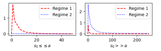
Figure 1: Regimes in RSGD for Sparse PCA

7.2 Low Rank Matrix Completion

$$\begin{array}[]{rl}\min\limits_{X\in\mathcal{M}}&\sum\limits_{i,j}|A_{ij}-X_{ij}|\\ &\mathcal{M}:=\{X\in\mathbb{R}^{m\times n},\,\mathop{rank}(X)=p\}\end{array}$$ (32)

In order to make the problem stochastic we consider that access to the components of $A$ is noisy, i.e., every evaluation of $A_{ij}$ is of the form $A_{ij}+\epsilon$ where $\epsilon\sim\mathcal{N}(0,\sigma)$ for a small $\sigma$.

Here we have the results of using RSGD with diminishing step size according the same two regimes as in the above example. We consider a normalized random matrix of order $100\times 100$ with some noise $\epsilon$ on entries where $\epsilon\in\mathcal{N}(0,\sigma)$ and $\sigma=1\text{e}-3$.

We will do the experiment in $10$ epochs in which each $10^{4}$ times and plot the result in Figure 2 by the median method.

In the Figure 2, on the left side we have considered $a=s_{0}=10$ and $c=1$e-4 and on the right side $a=.1$, $s=1000$ and $c=$1e-4. The cost function ($y$-axis) starts to decrease rapidly as the number of iterates ($x$-axis) increases.

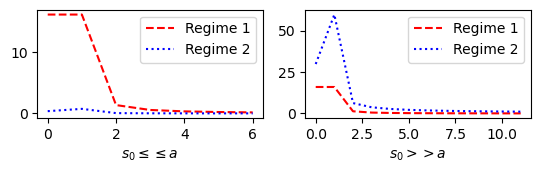
Figure 2: Regimes in RSGD: Low Rank Matrix Completion

We observe convergence for both step size regimes again.

7.3 ReLU Neural Network with Batch Normalization

Inspired by [16], we shall also consider the problem of training a neural network with batch normalization. We consider regression with a network composed of Rectified Linear Units (ReLUs), activation functions that take a component wise maximum between the previous layer, linearly transformed, and zero. For additional non smoothness, we consider an $l1$ loss function. Batch Normalization amounts to scaling the weights at each layer to encourage stability in training. Formally,

$$\begin{array}[]{rl}\min\limits_{w\in\mathcal{M}}&\frac{1}{N}\sum\limits_{i=1}^{N}|\hat{y}(x_{i};w)-y_{i}|\\ &\mathcal{M}:=\{x\in\mathbb{S}^{n_{1}}\times\mathbb{S}^{n_{2}}\times\cdots\times\mathbb{S}^{n_{L}}\times\mathbb{R}^{n_{o}}\}\end{array}$$ (33)

where we have $N$ training examples $\{x_{i},y_{i}\}$ and $\hat{y}$ is the neural network model given the set of weights $w$, at each layer $j=1,...,L$, there are $n_{j}$ weights to be normalized, and there are $n_{0}$ additional unnormalized weights.

We are reporting the result of the experiment on two data sets:

The first one is from sklearn data sets regression: ”$load~{}digits$” in which the number of digit numbers is $N=1797$ and the number of features of each is $64$. We have $L=4$, therefore we will have a $4-$layers neural network, with $4$ weights and $4$ biases. The number of nodes in the hidden layers is of order $10\times 10$.

The second one is from LIBSVM library data sets regression: ”$eunite2001$” in which $N=367$ and the number of features of each is $16$, and the neural networks are the same as before.

Again, we will use the median method for plotting the Figure 3 and 4, for the number of $10$ epochs and each $10^{4}$ iterations. We use the same two step size regimes as before.

We see, in Figures 3 and 4, the loss of the neural network ($y$-axis) is decreasing as the number of iterations ($x$-axis) increases. The loss will be a constant but not necessarily approaching zero. For both step size regimes we have a rapid decrease, with regime 1 performing better than regime 2.

Here in Figure 3 we use $a=s_{0}=10,$ a small constant $c=1\text{e}-4$, and a random batch size = 16. We can see in both data sets that regime 1 is performing better than regime 2.

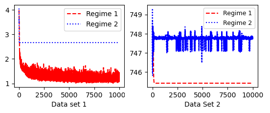
Figure 3: Regimes in RSGD for Batch Normalization

We should notice that the regime’s efficiency is sensitive to the parameters $a,~{}s_{0}$, and $c$. For instance, for the same batch size=16 and a small constant $c=1$e-4, if $s_{0}=10$ and $a=0.1$, in Figure 4 the regime 2 results in more oscillation on data set 1 and performing better on data set 2 than data set 1.

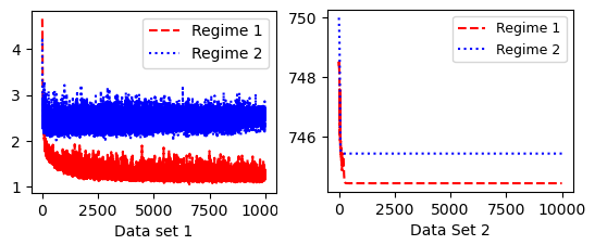
Figure 4: Regimes in RSGD for Batch Normalization

We notice, the larger the minibatch the smaller the noise. This fact can be verified by choosing two mini batch sizes and parameters $a=s_{0}=10$ and $c=1$e-4, in the following Figure 5. Note in particular the results corresponding to regimes 1 and 2 in data set 1, and regime 2 in data set 2.

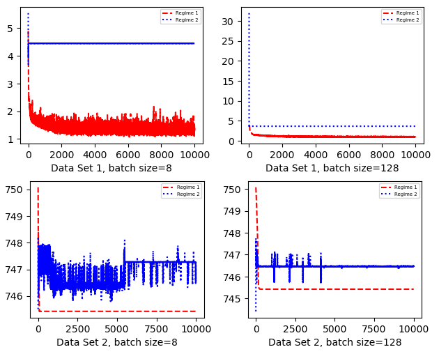
Figure 5: Noises based on batch sizes in RSGD

8 Discussion and Conclusions

Both tame geometry, as a structural topological description of an important class of so-called Whitney-stratifiable functions, and Riemannian geometry, as precise geometric modeling of structural constraints, are simultaneously mathematically elegant as well as increasingly important in faithfully modeling important problems arising in machine learning. As such their combination is an important open problem that this paper has addressed. A number of conceptual challenges had to be addressed to adequately studying algorithms in this space, requiring significant generalizations of stochastic approximation techniques. We intend that this opens an expansive space of potential work studying other existing algorithms as well as insight to develop new ones.

blabla

9 Appendix: Proofs

The proofs of Theorems 4.4, 4.9 and 4.10 are trivially lifted from the references to the Riemannian setting, and we do not include them here.

Proof of theorem 4.5.

We follow the procedure in [4]. Fix a measurable selection $a\,:\,\mathcal{M}\to T^{*}\mathcal{M}$ of $D$ and a potential $f$ of $D$. Further, fix a point $x\in\mathcal{M}$, a vector $v\in T_{x}\mathcal{M}$ and let $\gamma(t)\,:\,[0,1]\to\mathcal{M}$ be the curved defined by $\gamma(0)=x$ and $\dot{\gamma}(0)=v$.

The definition of a potential function gives us

$$f(\gamma(1))-f(x)=\int_{0}^{1}\langle a(\gamma(t)),\dot{\gamma}(t)\rangle\mathrm{d}t,$$ (34)

giving us $df_{x}(v)=\lim_{t\to 0}\frac{f(\gamma(t))-f(x)}{t}=\langle a,v\rangle$ almost everywhere along $\gamma(t)$, since Rademacher’s theorem says that $f$ is differentiable almost everywhere.

Introduce the Dini derivatives [12]

$$f^{\prime}_{u}(y;v)\coloneqq\limsup_{t\to 0^{+}}\frac{f(\gamma(t))-f(x)}{t},$$ (35)

$$f^{\prime}_{l}(y;v)\coloneqq\liminf_{t\to 0^{+}}\frac{f(\gamma(t))-f(x)}{t}.$$

Since $f$ is measurable, $f^{\prime}_{u}$ and $f^{\prime}_{l}$ are as well. Now, consider the set

$$\footnotesize A=\{y\in\mathcal{M}\,:\,f^{\prime}_{u}(y;v)\neq\langle a(y),v\rangle\text{ or }f^{\prime}_{l}(y;v)\neq\langle a(y),v\rangle\}.$$ (36)

This set is measurable and for $y\in\mathcal{M}\backslash A$ and $v\in T_{y}\mathcal{M}$ we have

$$df_{y}(v)=f^{\prime}_{u}(y;v)=f^{\prime}_{l}(y;v)=\langle a(y),v\rangle.$$ (37)

Furthermore, $\lambda(A\cap\gamma(I))=0$, with $I=[0,1]$. Fubini’s theorem then tells us that $\lambda(A)=0$. Both $x$ and $v$ were chosen at random and we can run the same argument for any $x\in\mathcal{M}$ and any $v\in T_{x}\mathcal{M}$, then we see that $df_{y}=a(y)$ for almost all $y\in\mathcal{M}$.

Furthermore, the selection $a$ was chosen arbitrarily and Corollary 18.15 of [1] then tells us that there exists a sequence of measurable selections $(a_{k})_{k\in\mathbb{N}}$ of $D$ such that for any $x\in\mathcal{M}$ $D(x)=\overline{\{a_{k}(x)\}}_{k\in\mathbb{N}}$. Rademacher again tells us that there exists a sequence of measurable sets $(S_{k})_{k\in\mathbb{N}}$ with full measure and such that $a_{k}=df$ on each $S_{k}$. Setting $S=\bigcap_{k\in\mathbb{N}}S_{k}$ we have that $\mathcal{M}\backslash S$ has zero measure and this implies that $D=\{df\}$ on $S$.

∎

9.1 Proof of Theorem 6.2

For later reference, let us state the following definitions.

Definition 9.1 (Attracting set, [2]).

Given a closed invariant set $L$, the induced set-valued dynamical system $\Phi^{L}$ is the family of set-valued mappings $\Phi_{L}=\{\Phi_{t}^{L}\}_{t\in\mathbb{R}}$ defined by

$$\Phi_{t}^{L}(x)\coloneqq\{ \gamma(t)\,:\,\gamma(t)\text{ is a solution of \eqref{eq:diffInclusion} with }$$ (38)

$$\gamma(0)=x\text{ and }\gamma(\mathbb{R})\subset L\}.$$

A compact subset $A\subset L$ is called an attracting set for $\Phi^{L}$, provided that there is a neighborhood $U$ of $A$ in $L$ with the property that for any $\varepsilon>0$ there exists $t_{\varepsilon}>0$ such that

$$\Phi_{t}^{L}(U)\subset\bigcup_{x\in A}B(x,\varepsilon),\quad\forall t>t_{\varepsilon}.$$ (39)

If $A$ is an invariant set, then $A$ is called an attractor for $\Phi^{L}$. Note that, an attracting set (or attractor) for $\Phi$ is an attracting set (or attractor) for $\Phi^{L}$ with $L=\mathcal{M}$. If $A\neq L,\,\varnothing$, then $A$ is called a proper attracting set (or attractor) for $\Phi^{L}$. Finally, the set $U$ is referred to as a fundamental neighborhood of $A$ for $\Phi^{L}$.

Definition 9.2 (Asymptotic stability, [2]).

A set $A\subset L$ is called asymptotically stable for $\Phi^{L}$ if it satisfies the following:

1. $A$ is invariant;

2. $A$ is Lyapunov stable, meaning that for every neighborhood $U$ of $A$ there exists a neighborhood $V$ of $A$ such that $\Phi_{[0,\infty)}(V)\subset U$;

3. $A$ is attractive, i.e., there exists a neighborhood $U$ of $A$, such that for any $x\in U$ we have $\omega_{\Phi}(x)\subset A$.

The set

$$\omega_{\Phi}(x)\coloneqq\bigcap_{t\geq 0}\overline{\Phi_{[t,\infty)}(x)}$$ (40)

is the $\omega$-limit set of a point $x\in\mathcal{M}$.

We now have the following results from [2]:

Theorem 9.3 (Theorem 4.1 in [2]).

Assume $\zeta$ is bounded. Then the following two statements are equivalent:

1. $\zeta$ is an APT for $\Phi$;

2. $\zeta$ is uniformly continuous and any limit point of $\{\Theta^{t}(\zeta)\}$ is in $\mathcal{S}$.

In both cases the set $\{\Theta^{t},\,t\geq 0\}$ is relatively compact.

Proof.

The proof is essentially the same as in [2]. Since $K=\{\zeta(t):\,t\geq 0\}$ is compact, by assumption, for any $\varepsilon>0$ there exists $\eta>0$ such that $d(\zeta,\gamma)<\varepsilon$, for any $\gamma\in K$, $\zeta\in\Phi_{s}(\gamma)$ and $|s|<\eta$. This follows from the fact that $(x,t)\mapsto\Phi_{t}(x)$ has compact values. If $\zeta$ is an APT there exists some $T$ such that $t>T$ implies

$$d_{C}(\zeta(t+s),\Phi_{s}(\zeta(t))<\frac{\varepsilon}{2},\qquad\forall|s|<\eta.$$ (41)

This further implies that $d(\zeta(t+s),\zeta(t))\leq\varepsilon$ and $\zeta$ is thus uniformly continuous. Due to the defining property (30) every limit point will belong to $\mathcal{S}$.

If, on the other hand, $\zeta$ is uniformly continuous, then the family of functions $\{\Theta^{t}(\zeta)\,:\,t\geq 0\}$ is equicontinuous and the Arzelà-Ascoli theorem then tells us that the family is relatively compact, and (30) follows. ∎

Theorem 9.4 (Theorem 4.2 in [2]).

Any bounded perturbed solution $\tilde{\gamma}$ is an APT of the differential inclusion (21).

Proof.

We prove that $\tilde{\gamma}$ satisfies the second point in Theorem 9.3. To this end, set $v(t,s)=P^{u_{t}}_{\tilde{\gamma}(t)u_{t}(s)}\dot{\tilde{\gamma}}(t)-\dot{u}_{t}(s)\in G^{\delta(t)}(\tilde{\gamma}(t))$. Then,

$$d(\tilde{\gamma}(t_{1}+t_{2}),\tilde{\gamma}(t_{1}))$$ (42)

$$= \int_{T_{t_{1}}}^{T_{t_{1}+t_{2}}}\int_{0}^{t_{2}}\left\lVert v(t_{2}+\tau,s)\right\rVert_{g_{u_{t_{2}+\tau}(s)}}\mathrm{d}\tau\mathrm{d}s$$

$$+\int_{T_{t_{1}}}^{T_{t_{1}+t_{2}}}\int_{t_{1}}^{t_{1}+t_{2}}\left\lVert\dot{u}_{\tau}(s)\right\rVert_{g_{u_{\tau}(s)}}\mathrm{d}\tau\mathrm{d}s.$$

By the defining properties of $u_{t}$ the second integral goes to zero as $t\to\infty$. The boundedness of $\tilde{\gamma}$, $\tilde{\gamma}(\mathbb{R})\in A$ for compact $A$ then implies the boundedness of $v$ and we thus see that $\tilde{\gamma}$ is uniformly continuous. Thus, $\Theta^{t}(\tilde{\gamma})$ is equicontinuous, and relatively compact. Let $\zeta=\lim_{n\to\infty}\Theta^{t_{n}}(\tilde{\gamma})$ be a limit point, set $t_{1}=r_{n}$ above (42) and define $v_{n}(t_{2},s)=v(r_{n}+t_{2},s)$. Again, by the defining properties of $u_{t}$ the second integral in (42) will vanish uniformly when $n\to\infty$. Hence,

$$d(\zeta(t_{2}),\zeta(0))=\lim_{n\to\infty}\int_{T_{r_{n}}}^{T_{r_{n}}+T_{t_{2}}}\int_{0}^{t_{2}}\left\lVert v_{n}(\tau)\right\rVert_{g_{u_{r_{n}+\tau}(s)}}\mathrm{d}\tau\mathrm{d}s.$$ (43)

∎

Since $(v_{n})$ is uniformly bounded, Banach-Alaoglu tells us that a subsequence of $v_{n}$ will converge weakly in $L^{2}[0,t_{2}]$ to some function $v$ with $v(t)\in G(\zeta(t))$, for almost any $t$, since $v_{n}(t)\in G^{\delta(t+r_{n})}(\tilde{\gamma}(t+r_{n}))$ for every $t$. Now, a convex combination of $\{v_{m},\,m>n\}$ converges almost surely to $v$, by Mazur’s lemma, and $\lim_{m\to\infty}\text{conv}\left(\bigcup_{n\geq m}G^{\delta(t+r_{n})}(\tilde{\gamma}(t+r_{n}))\right)\subset G(\zeta(t))$. We thus have that $d(\zeta(t_{2}),\zeta(0))=\int_{T_{t_{1}}}^{T_{t_{1}}+T_{t_{2}}}\int_{0}^{t_{2}}\left\lVert v(\tau,s)\right\rVert_{g_{u_{\tau}}(s)}\mathrm{d}\tau\mathrm{d}s$. This proves that $\zeta$ is a solution of (21) and that $\zeta\in\widehat{\mathcal{S}}_{A}$.

Theorem 9.5 (Theorem 4.3 in [2]).

Let $\zeta$ be a bounded APT of (21). Then $L(\zeta)$ is internally chain transitive.

Proof.

The proof is more or less identical to that of [2]. The set $\{\Theta^{t}(\zeta)\,:\,t\geq 0\}$ is relatively compact, and the $\omega$-limit set of $\zeta$ for the flow $\Theta$,

$$\omega_{\Theta}(\zeta)=\bigcap_{t\geq 0}\overline{\{\Theta^{s}(\zeta)\,:\,s\geq t\}},$$ (44)

is therefore internally chain transitive. From (30) we know that $\omega_{\Theta}(\zeta)\subset\mathcal{S}$.

Let $\Pi\,:\,(C^{0}(\mathbb{R},\mathcal{M}),d_{C})\to(\mathcal{M},d(\cdot,\cdot))$ be the projection map defined by $\Pi(\zeta)=\zeta(0)$. This gives $\Pi(\omega_{\Theta}(\zeta))=L(\zeta)$. Now, set $p=\lim_{n\to\infty}\zeta(t_{n})$ and $w$ a limit point of $\Theta^{t_{n}}(\zeta)$, then $w\in\omega_{\Theta}(\zeta)$ and $\Pi(w)=p$. This implies that $L(\zeta)$ is nonempty, compact and invariant under $\Phi$, since $\omega_{\Theta}(\zeta)\subset\mathcal{S}$. The projection $\Pi$ has Lipschitz constant one and maps every $(\varepsilon,T)$ chain for $\Theta$ to an $(\varepsilon,T)$ chain for $\Phi$. This means that $L(\zeta)$ is internally chain transitive. ∎

We will prove the following theorem, which in turn will imply Theorem 6.2. The proof follows that of Theorem 3.2 in [8].

Theorem 9.6.

Suppose that assumption 6.1 holds and that there exists a Lyapunov function $\varphi$ on $\mathcal{M}$. Then every limit point of $\{x_{k}\}_{x\geq 1}$ lies in $G^{-1}(0)$ and the function values $\{\varphi(x_{k})\}_{k\geq 1}$ converge.

We will need the following lemmas.

Lemma 9.7.

$\lim_{k\to\infty}d(x_{k},x_{k+1})=0$

Proof.

The retraction is a smooth map from $T\mathcal{M}\to\mathcal{M}$ and we have $D\mathcal{R}_{x}(0_{x})[v]=v$. Furthermore, we can define a curve $\gamma(t)=\mathcal{R}_{x}(tv)$, $\dot{\gamma}(0)=v$ and $\mathcal{R}_{x}(0_{x})=x$. Now,

$$\left\lVert v\right\rVert_{g_{x}}\leq\alpha_{k}\max_{z\in F(x_{k})}\left\lVert z\right\rVert_{g_{x}}+\alpha_{k}\left\lVert\dot{u}_{t}\right\rVert_{g_{x}}.$$ (45)

But the second part goes to zero by assumption and $\left\lVert z\right\rVert_{g_{x}}$ is bounded while $\alpha_{k}\to 0$, so this implies that $v$ converges to zero and therefore $d(x_{k},x_{k+1})\to 0$, since $\mathcal{R}(tv)$ is smooth. ∎

Lemma 9.8.

We have

$$\liminf_{t\to\infty}\varphi(x(t))=\liminf_{k\to\infty}\varphi(x_{k}),$$ (46)

and

$$\limsup_{t\to\infty}\varphi(x(t))=\limsup_{k\to\infty}\varphi(x_{k}).$$ (47)

Proof.

Clearly, we have that $\leq$ and $\geq$ holds, respectively, in the two equations. To argue for the opposite direction we let $\tau_{i}\to\infty$ be an arbitrary sequence with $x(\tau_{i})$ converging to some point $x^{*}$ as $i\to\infty$. For each index $i$, we define the breakpoint $k_{i}=\max\{k\in\mathbb{N}\,:\,t_{k}\leq\tau_{i}\}$. Then

$$d(x_{k_{i}},x^{*})\leq d(x_{k_{i}},x(\tau_{i}))+d(x(\tau_{i}),x^{*})$$ (48)

$$\leq d(x(\tau_{i}),x^{*})+d(x_{k_{i}},x_{k_{i}+1}).$$

Since the right hand side tends to zero we get that $x_{k_{i}}\to x^{*}$, which further implies that $\varphi(x_{k_{i}})\to\varphi(x^{*})$.

Let now $\tau_{i}\to\infty$ be a sequence realizing $\liminf_{t\to\infty}\varphi(x(t))$. Since $x(t)$ is bounded, $x(\tau_{i})$ converges to some point $x^{*}$ and we find

$$\liminf_{k\to\infty}\varphi(x_{k})\leq\lim_{i\to\infty}\varphi(x_{k_{i}})=\varphi(x^{*})=\liminf_{t\to\infty}\varphi(x(t)).$$ (49)

The second equality can be shown in the same way. ∎

Proposition 9.9.

The values $\varphi(x(t))$ have a limit as $t\to\infty$.

Proof.

Without loss of generality, suppose $0=\liminf_{t\to\infty}\varphi(x(t))$. For each $r\in\mathbb{R}$, define the sublevel set

$$L_{r}\coloneqq\{x\in\mathcal{M}\,:\,\varphi(x)\leq r\}.$$ (50)

Choose any $\varepsilon>0$ satisfying $\varepsilon\notin\varphi(G^{-1}(0))$. Note that $\varepsilon$ can be arbitrarily small. According to the above lemma we then have infinitely many indices $k$ such that $\varphi(x_{k})<\varepsilon$. Then, for sufficiently large $k\in\mathbb{N}$ we have

$$x_{k}\in L_{\varepsilon}\implies x_{k+1}\in L_{2\varepsilon}.$$ (51)

This follows from the same argument as in [8].

Let us define a sequence of iterates. Set $i_{1}\in\mathbb{N}$ as the first index satisfying

1. $x_{i_{1}}\in L_{\varepsilon}$;

2. $x_{i+1}\in L_{2\varepsilon}\backslash L_{\varepsilon}$;

3. defining the exit time $e_{1}=\min\{e\geq i_{1}\,:\,x_{e}\notin L_{2\varepsilon}\backslash L_{\varepsilon}\}$, the iterate $x_{e_{1}}$ lies in $\mathcal{M}\backslash L_{2\varepsilon}$.

Next, let $i_{2}>i_{1}$ be the next smallest index satisfying the same properties, and so on. This process must then terminate, i.e., $\{x_{k}\}$ exits $L_{2\varepsilon}$ a finite amount of times. Then we see that the proposition follows, since $\varepsilon$ can be made arbitrarily small and the above lemma gives us $\lim_{t\to\infty}\varphi(x(t))=0$. ∎

Now we can give the proof of the theorem.

Proof of Theorem 9.6.

Let $x^{*}$ be a limit point of $\{x_{k}\}$ and suppose for the sake of contradiction that $0\notin G(x^{*})$. Let $i_{j}$ be indices satisfying $x_{i_{j}}\to x^{*}$ as $j\to\infty$. Let $z(\cdot)$ be the subsequential limit of the curves $\gamma^{t_{i_{j}}}(\cdot)$ in $C(\mathbb{R}_{+},\mathcal{M})$ which are guaranteed to exist. The existence of the Lyapunov function guarantees that there exists a real $T>0$ satisfying

$$\varphi(z(T))<\sup_{t\in[0,T]}\varphi(z(t))\leq\varphi(x^{*}).$$ (52)

But, we can deduce

$$\varphi(z(T))=\lim_{j\to\infty}\varphi(\gamma^{t_{i_{j}}}(T))=\lim_{t\to\infty}\varphi(\gamma(t))=\varphi(x^{*}),$$ (53)

where we used the above proposition and continuity of $\varphi$ in the last step. But this is a contradiction and the theorem follows. ∎

10 Appendix: The Clarke Subdifferential on a Manifold

A central object in non-smooth analysis is the Clarke subdifferential. We define it for a Riemannian manifold following [15]. To this end, we first define the generalized directional derivative.

Definition 10.1 (Generalized directional derivative and Clarke subdifferential).

Let $f\,:\,\mathcal{M}\to\mathbb{R}$ be a locally Lipschitz function and $(U,\varphi)$ a chart at $x\in\mathcal{M}$. The generalized directional derivative of $f$ at $x$ in the direction $v\in T_{x}\mathcal{M}$, denoted $f^{\circ}(x;v)$, is then defined by

$$f^{\circ}(x;v)\coloneqq\limsup_{y\to x,t\searrow 0}\tfrac{f\circ\varphi^{-1}(\varphi(y)+t\mathrm{d}\varphi(x)(v))-f\circ\varphi^{-1}(\varphi(y))}{t}.$$ (54)

The Clarke subdifferential of $f$ at $x$, denoted $\partial f(x)$, is furthermore the subset of $T^{*}_{x}\mathcal{M}$ whose support function is $f^{\circ}(x;\cdot)$.

The Clarke subdifferential gives a minimal convex conservative field, as is seen by the following.

Theorem 10.2 (Cf. Corollary 1 in [4]).

Let $f\,:\,\mathcal{M}\to\mathbb{R}$ allowing a conservative field $D\,:\,\mathcal{M}\rightrightarrows T^{*}\mathcal{M}$. Then $\partial f$ is a conservative field for $f$, and for all $x\in\mathcal{M}$

$$\partial f(x)\subset\text{conv}\,(D(x)).$$ (55)

Proof.

The idea is the same as in the proof of Corollary 1 in [4]. Fix an $S\subset\mathcal{M}$, a full measure set such that $D=\mathrm{d}f$ on $S$. From Lemma 5.5 of [15] we have

$$\partial f(x)=\overline{\text{co}}\{\lim_{k\to\infty}\mathrm{d}f(x_{k})\,:\,\{x_{k}\}\subset S,\,x_{k}\to x\}.$$ (56)

But $D$ has a closed graph and on $S$ we have $D=\mathrm{d}f$, so the result follows directly. ∎

11 Appendix: O-minimal Structures

For reference, we give the definition of o-minimal structures and list a few important examples. For more information we refer to [25, 26].

Definition 11.1 (O-minimal structure).

An o-minimal structure on $\mathbb{R}$ is a sequence $\mathcal{S}=(\mathcal{S}_{m})_{m\in\mathbb{N}}$ such that for each $m\geq 1$:

1. $\mathcal{S}_{m}$ is a boolean algebra of subsets of $\mathbb{R}^{m}$;

2. if $A\in\mathcal{S}_{m}$, then $\mathbb{R}\times A$ and $A\times\mathbb{R}$ belongs to $\mathcal{S}_{m+1}$;

3. $\{(x_{1},\dots,x_{m})\in\mathbb{R}^{m}\,:\,x_{1}=x_{m}\}\in\mathcal{S}_{m}$;

4. if $A\in\mathcal{S}_{m+1}$, and $\pi:\,\mathbb{R}^{m+1}\to\mathbb{R}^{m}$ is the projection map on the first $m$ coordinates, then $\pi(A)\in\mathcal{S}_{m}$;

5. the sets in $\mathcal{S}_{1}$ are exactly the finite unions of intervals and points.

A set $A\subseteq\mathbb{R}^{m}$ is said to be definable in $\mathcal{S}$, or $\mathcal{S}$-definable, if $A$ belongs to $\mathcal{S}_{m}$. Similarly, a map $f:\,A\to B$, with $A\subseteq\mathbb{R}^{m}$, $B\subseteq\mathbb{R}^{n}$, is said to be definable in $\mathcal{S}$ if its graph $\Gamma(f)\subseteq\mathbb{R}^{m+n}$ belongs to $\mathcal{S}_{m+n}$. When we do not wish to specify any particular structure we simply say that a definable function or set is tame.

Some important examples of o-minimal structures are:

• The collection of semi-algebraic sets forms an o-minimal structure denoted $\mathbb{R}_{\text{semialg.}}$.

• Adjoining the collection of semi-algebraic sets with the graph of the real exponential function, $x\mapsto e^{x}$, $x\in\mathbb{R}$, gives an o-minimal structure denoted $\mathbb{R}_{\text{exp.}}$.

• The collection of restricted analytic functions can also be adjoined with $\mathbb{R}_{\text{semialg.}}$ to give the o-minimal structure $\mathbb{R}_{\text{an.}}$.

• Finally, we can actually combine $\mathbb{R}_{\text{exp.}}$ with $\mathbb{R}_{\text{an.}}$ to get the o-minimal structure $\mathbb{R}_{\text{an.,exp.}}$.

References

- [1] C.D Aliprantis and K.C. Border. Infinite dimensional analysis: A hitchhikers guide.
- [2] Michel Benaïm, Josef Hofbauer, and Sylvain Sorin. Stochastic approximations and differential inclusions. SIAM Journal on Control and Optimization, 44(1):328–348, 2005.
- [3] Pascal Bianchi, Walid Hachem, and Sholom Schechtman. Convergence of constant step stochastic gradient descent for non-smooth non-convex functions. Set-Valued and Variational Analysis, pages 1–31, 2022.
- [4] Jérôme Bolte and Edouard Pauwels. Conservative set valued fields, automatic differentiation, stochastic gradient methods and deep learning. Mathematical Programming, 188(1):19–51, 2021.
- [5] Jérôme Bolte, Aris Daniilidis, and Adrian Lewis. Tame functions are semismooth. Math. Program., 117:5–19, 03 2009.
- [6] Vivek S Borkar. Stochastic approximation: a dynamical systems viewpoint, volume 48. Springer, 2009.
- [7] Annegret Y. Burtscher. Length structures on manifolds with continuous riemannian metrics. arXiv: Differential Geometry, 2012.
- [8] Damek Davis, Dmitriy Drusvyatskiy, Sham Kakade, and Jason D Lee. Stochastic subgradient method converges on tame functions. Foundations of computational mathematics, 20(1):119–154, 2020.
- [9] Fabio V Difonzo, Vyacheslav Kungurtsev, and Jakub Marecek. Stochastic langevin differential inclusions with applications to machine learning. arXiv preprint arXiv:2206.11533, 2022.
- [10] Alain Durmus, Pablo Jiménez, Éric Moulines, Salem Said, and Hoi-To Wai. Convergence analysis of riemannian stochastic approximation schemes. arXiv preprint arXiv:2005.13284, 2020.
- [11] Alain Durmus, Pablo Jiménez, Éric Moulines, and SAID Salem. On riemannian stochastic approximation schemes with fixed step-size. In International Conference on Artificial Intelligence and Statistics, pages 1018–1026. PMLR, 2021.
- [12] Orizon P Ferreira. Dini derivative and a characterization for lipschitz and convex functions on riemannian manifolds. Nonlinear Analysis: Theory, Methods & Applications, 68(6):1517–1528, 2008.
- [13] Najmeh Hoseini Monjezi, Soghra Nobakhtian, and Mohamad Reza Pouryayevali. A proximal bundle algorithm for nonsmooth optimization on riemannian manifolds. IMA Journal of Numerical Analysis, 2021.
- [14] S Hosseini and MR Pouryayevali. Nonsmooth optimization techniques on riemannian manifolds. Journal of Optimization Theory and Applications, 158(2):328–342, 2013.
- [15] Seyedehsomayeh Hosseini and M. Pouryayevali. Generalized gradients and characterization of epi-lipschitz sets in riemannian manifolds. Nonlinear Analysis, 74:3884–3895, 08 2011.
- [16] Jiang Hu, Xin Liu, Zai-Wen Wen, and Ya-Xiang Yuan. A brief introduction to manifold optimization. Journal of the Operations Research Society of China, 8(2):199–248, 2020.
- [17] Hideaki Iiduka and Hiroyuki Sakai. Riemannian stochastic fixed point optimization algorithm. Numerical Algorithms, pages 1–25, 2022.
- [18] Vyacheslav Kungurtsev, Francesco Rinaldi, and Damiano Zeffiro. Retraction based direct search methods for derivative free riemannian optimization. arXiv preprint arXiv:2202.11052, 2022.
- [19] Yuri Ledyaev and Qiji Zhu. Nonsmooth analysis on smooth manifolds. Transactions of the American Mathematical Society, 359:3687–3732, 08 2007.
- [20] John M Lee and John M Lee. Smooth manifolds. Springer, 2012.
- [21] Szymon Majewski, Błażej Miasojedow, and Eric Moulines. Analysis of nonsmooth stochastic approximation: the differential inclusion approach. arXiv preprint arXiv:1805.01916, 2018.
- [22] Xavier Pennec. Probabilities and statistics on riemannian manifolds: A geometric approach. PhD thesis, INRIA, 2004.
- [23] M. Pouryayevali and Hajar Radmanesh. Trajectories of differential inclusions on riemannian manifolds and invariance. Set-Valued and Variational Analysis, 27, 03 2019.
- [24] Suhail M Shah. Stochastic approximation on riemannian manifolds. Applied Mathematics & Optimization, 83(2):1123–1151, 2021.
- [25] Lou van den Dries. Tame topology and o-minimal structures, volume 248. Cambridge university press, 1998.
- [26] Lou van den Dries and Chris Miller. Geometric categories and o-minimal structures. Duke Mathematical Journal, 84:497–540, 1996.