Temperature gradient and asymmetric steady state correlations in dissipatively coupled cascaded optomechanical systems

Abstract

The interaction between a light mode and a mechanical oscillator via radiation pressure in optomechanical systems is an excellent platform for a multitude of applications in quantum technologies. In this work we study the dynamics of a pair of optomechanical systems interacting dissipatively with a wave guide in a unidirectional way. Focusing on the regime where the cavity modes can be adiabatically eliminated we derive an effective coupling between the two mechanical modes and we explore both classical and quantum correlations established between the modes in both in the transient and in the stationary regime, highlighting their asymmmetrical nature due to the unidirectional coupling, and we find that a constant amount of steady correlations can exist at long times. Furthermore we show that this unidirectional coupling establishes a temperature gradient between the mirrors, depending on the frequencies’ detuning. We additionally analyze the power spectrum of the output guide field and we show how, thanks to the chiral coupling, from such spectrum it is possible to reconstruct the spectra of each single mirror.

I Introduction

Optomechanical systems, with light modes interacting with massive mechanical oscillators, have attracted a considerable interest for their possible application in quantum technologies [1, 2]. Depending on the working point, the optomechanical interaction can be used to cool the mechanical mode near to its ground state [3, 4, 5, 6, 7, 8] (a technique applied also to levitating nanospheres [9]), to generate squeezing [10, 11, 12] or to create entanglement between optical and mechanical modes [13, 14, 15]. These configurations can be mixed in an appropriate way in order to generate purely quantum states of the mechanical oscillators (e.g. generation of single phonon states [16]).

A natural extension of the standard single mode - single mirror oscillators setups consists of several coupled modes. We can distinguish two major and distinct setups. The first one is called Multimode optomechanical system [17, 18, 19, 20, 21], and consists of several mechanical oscillator interacting with the same cavity. In Optomechanical array instead, each mechanical oscillator interacts locally with its own cavity-mode but an effective coupling between neighbouring mirrors is implemented by photons and/or phonons tunneling [22, 23, 24].

In this work we propose the largely unexplored setup in which the cavity modes are dissipatively coupled via a unidirectional waveguide [25] in a cascaded configuration [26, 27, 28, 29, 30]. This arrangement induces a non-reciprocal interaction, at first between the cavities and then between the mechanical oscillators [31]. While previous studies have explored similar setups, none of them has specifically addressed pure unidirectional coupling [32]. For instance, in [33, 34], the authors study the synchronization between two resonators driven by a blue detuned laser, which leads to a self-sustained oscillatory dynamics and in [35] the possibility of creating non-reciprocal devices that control the flow of thermal noise towards or away from specific quantum devices in a network has been explored. However, in spite of the above, the full potential of cascaded coupling between a pair of optomechanical systems remains largely unexplored, especially when it comes to the effective coupling between the two mechanical modes. To fill this gap, we derive the equations describing the effective coupling between the two mirrors by adiabatically eliminating the cavity modes. We then characterise the correlations established between the mirrors in terms of mutual information and quantum discord, the latter being the best quantifier when one is interested in asymmetries between the two mirrors. We show that asymmetric non-zero correlations persists even in the steady state. Additionally, we explore the consequences of the asymmetry in the coupling, arising from the unidirectionality, and its implications for establishing a temperature gradient between the two modes. Notably, this temperature gradient vanishes in the case of perfectly symmetrical bidirectional coupling.

This work is organized as follow: In section II we present our model, we introduce its Hamiltonian. By employing Langevin equations we characterise the evolution of the system in terms of mean values and fluctuations. The fluctuations are further analysed using Lyapunov equation for the covariance matrix. In section III, we derive an equation of motion for the effective dynamics of the two mechanical oscillators. This is achieved by performing an adiabatic elimination of the cavity modes. In section IV, we investigate the correlations between the two mechanical modes through the evaluation of mutual information and quantum discord. Interestingly, we find that these asymmetric correlations (Discord) retain non-zero values even in the stationary state, indicating the potential for establishing persistent correlations. In section V, we show how, in the cooling regime, the unidirectional coupling leads to the thermalization of the two mechanical modes at different temperatures, depending on the frequency mismatch of the mirrors. This reveals the so far unexplored setup to engineer a temperature gradient using the cascaded configuration. Section VI focuses on the analysis of the power spectra of the two mirrors and the output field mode, establishing the relationship between them. In section VII we study the stability regions of the parameters space, exploring when the system can exhibit multistability. Finally in section VIII we draw our conclusions.

II The system: two cascaded optomechanical cavities

Our system consists of two optomechanical mirrors each coupled to the same unidirectional waveguide. Such mediated indirect interaction (see fig. 1) leads to a cascade scenario in which the first system drives the following one without back action. Each subsystem consists of a mechanical harmonic oscillator with mass $m$ and frequency $\Omega_{j}$ coupled to a cavity field by means of its radiation pressure. As $\Omega_{j}$ is much smaller than $c/2L$ ($c$ is the speed of light and $L$ stands for the cavity length) we can consider a single cavity mode [36, 37] and write the following Hamiltonian for both subsystems:

$$\hat{H}_{S}=\sum_{j=1}^{2}\hat{H}_{j}=\sum_{j=1}^{2}\hbar\omega_{c}\hat{a}_{j}^{\dagger}\hat{a}_{j}{+}\dfrac{\hbar\Omega_{j}}{2}(\hat{q}_{j}^{2}{+}\hat{p}_{j}^{2})-\hbar g_{j}\hat{a}_{j}^{\dagger}\hat{a}_{j}\hat{q}_{j}+i\hbar E_{j}(\hat{a}_{j}^{\dagger}e^{-i\omega_{L}t}{-}\hat{a}_{j}e^{i\omega_{L}t})$$ (1)

where $\hat{a}_{j}$ is the cavity mode annihilation operator with optical frequency $\omega_{c}$ of the $j$-th subsystem and $\hat{q}_{j}$ ($\hat{p}_{j}$) stands for dimensionless position (momentum) operators of mechanical mode. The term proportional to $g_{j}{=}\omega_{c}/L\sqrt{\hbar/(m\Omega_{j})}$ describes the optomechanical coupling, while the last term is the coherent input field with frequency $\omega_{L}$. The quantities $E_{j}$ are related to the input powers $P_{j}$ by $E_{j}=\sqrt{2\kappa P_{j}/(\hbar\omega_{L})})$ where $\kappa$ is the cavity decay rate. In a rotating frame at laser frequency $\omega_{L}$, we define $\Delta=\omega_{c}-\omega_{L}$ and eq. 1 becomes

$$\hat{H}_{S}{=}\sum_{j}\hbar\left(\Delta-g_{j}\hat{q}_{j}\right)\hat{a}_{j}^{\dagger}\hat{a}_{j}{+}\frac{\hbar\Omega_{j}}{2}(\hat{q}_{j}^{2}{+}\hat{p}_{j}^{2})+i\hbar E_{j}(\hat{a}_{j}^{\dagger}-\hat{a}_{j})$$ (2)

In the following we focus on the scenario in which the dynamics of the second optomechanical system is driven only by the output field of the first cavity. Therefore, henceforth, we assume that the external laser pumps the first cavity only (i.e. $E_{2}=0$).

Due to the inherently open nature of our system, we consider that each mechanical mode is coupled to its respective environment, which is assumed to be at a finite temperature [38]. Additionally, we account for photon leakage from the cavities. Specifically, we assume that the optical dissipation occurs through a unidirectional waveguide, resulting in a cascade-like coupling between the two optical modes mediated by the interaction with the guide [31].

Following the standard input-output prescription of optical quantum Langevin equations [39], we introduce the radiation vacuum input noise operator $\hat{a}^{\text{in}}$ [40, 41] and the Brownian noise operator $\hat{\xi}_{j}$ [38] with autocorrelation functions:

$$\langle\hat{a}^{\text{in}}(t)\hat{a}^{\text{in}\dagger}(t^{\prime})\rangle=\delta(t-t^{\prime})$$ (3a)

$$\langle\{\hat{\xi}_{j}(t),\xi_{j}(t^{\prime})\}\rangle=\gamma_{j}(2\bar{n}_{j}+1)\delta(t-t^{\prime})$$ (3b)

where $\gamma_{j}$ denotes the decay rate of the j-th mirror and $\bar{n}_{j}=1/(\exp(\hbar\Omega_{j}/k_{B}T)+1)$ in which $k_{B}$ is the Boltzman constant and $T$ is the temperature of the mechanical modes’ bath. Although the cavity and the resonator are at the same temperature, however, the cavity frequency is typically orders of magnitude larger than the mechanical frequency, therefore the average number of photons in the optical environment is negligible. Based on the preceding analysis, we can derive the following quantum Langevin equations for the field operators $\hat{a}_{j}$:

$$\frac{d\hat{a}_{1}}{dt}=-\frac{i}{\hbar}[\hat{a}_{1},H_{S}]-\frac{\kappa}{2}\hat{a}_{1}-\sqrt{\kappa}\hat{a}^{\text{in}}$$ (4a)

$$\frac{d\hat{a}_{2}}{dt}=-\frac{i}{\hbar}[\hat{a}_{2},H_{S}]-\frac{\kappa}{2}\hat{a}_{2}-{\kappa}\hat{a}_{1}-\sqrt{\kappa}\hat{a}^{\text{in}}$$ (4b)

and the mirror operators $\hat{q}_{j}$, $\hat{p}_{j}$

$$\frac{d\hat{q}_{j}}{dt}=-\frac{i}{\hbar}[\hat{q}_{j},H_{S}]$$ (5a)

$$\frac{d\hat{p}_{j}}{dt}=-\frac{i}{\hbar}[\hat{p}_{j},H_{S}]-\gamma_{j}\hat{p}_{j}-\sqrt{\gamma_{j}}\,\hat{\xi}_{j}$$ (5b)

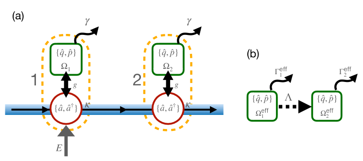
Figure 1: $(\mathbf{a})$ Sketch of the model involving two optomechanical systems: Each system consists of an optical mode and a mechanical mode, mutually interacting through the radiation pressure force induced by external laser power. We stress that these optomechanical systems are coupled to a unidirectional waveguide. In this context, the operators ${\hat{q},\hat{p}}$ represent the mechanical position and momentum, while ${\hat{a},\hat{a}^{\dagger}}$ are the creation and annihilation operators for the optical modes. The parameters $\gamma$ and $\kappa$ denote the mechanical and optical decay rates, respectively. Furthermore, $\Omega_{1,2}$ refer to the natural frequencies of the mechanical modes, and $g$ represents the coupling strength between the optical and mechanical modes due to radiation pressure. The amplitude of the coherent driving of the laser is denoted as $E$. ($\mathbf{b}$) Effective model describing the coupling between the mirrors, obtained by performing an adiabatic elimination of the optical modes. Within this framework, the effective frequencies of the mechanical modes are denoted as $\Omega^{\text{eff}}_{1,2}$, and $\Gamma^{\text{eff}}_{1,2}$ represents the effective decay rates. Moreover, $\Lambda$ (as defined in eq. 18) represents the cascaded effective coupling between the two mechanical modes.

Mean field equations and fluctuations Dynamics - The combined dynamics of the field-mirror system resulting from equations eq. 4 and eq. 5 is nonlinear. To investigate the quantum characteristics of optomechanical systems, a common method is to initially seek the mean field solution of the field and mechanical operators, and subsequently analyze the linearized dynamics of quantum fluctuations around these average values. Accordingly, we represent the operators as the sum of their average value (a $c$ number) and a small quantum fluctuation.

$$\hat{o}=\langle\hat{o}\rangle+[\hat{o}-\langle\hat{o}\rangle]=O+\delta\hat{o}$$ (6)

This leads to the following set of non linear differential equations for the mean values

$$\frac{dQ_{j}(t)}{dt}=\Omega_{j}P_{j}(t)$$ (7a)

$$\frac{dP_{j}(t)}{dt}=-\Omega_{j}Q_{j}(t)-\gamma_{j}P_{j}(t)+|G_{j}(t)|^{2}/g_{j}$$ (7b)

$$\frac{dA_{1}(t)}{dt}=-\frac{\kappa}{2}A_{1}(t)-i\Delta_{1}(t)A_{1}(t)+E$$ (7c)

$$\frac{dA_{2}(t)}{dt}=-\frac{\kappa}{2}A_{2}(t)-i\Delta_{2}(t)A_{2}(t)-\kappa A_{1}(t)$$ (7d)

where we defined $\Delta_{j}(t){=}\Delta{-}g_{j}Q_{j}(t)$ and $G_{j}(t){=}g_{j}A_{j}(t)$. It is important to note the inherent asymmetry in comparison to the bidirectional case (cfr. B). Solving eq. 7 and using eq. 6 into eqs. 4 and 5, we can write the following linearized set of equations for the fluctuations, where we keep only terms $\mathcal{O}(\delta\hat{o})$:

$$\frac{d\delta\hat{q}_{j}}{dt}=\Omega_{j}\delta\hat{p}_{j}$$ (8a)

$$\frac{d\delta\hat{p}_{j}}{dt}=-\Omega_{j}\delta\hat{q}_{j}+(G_{j}^{*}\delta\hat{a}_{j}+G_{j}\delta\hat{a}_{j}^{\dagger})-\gamma\delta\hat{p}_{j}-\xi_{j}$$ (8b)

$$\frac{d\delta\hat{a}_{1}}{dt}=iG_{1}\delta\hat{q}_{1}-i\Delta_{1}\delta\hat{a}_{1}-\frac{\kappa}{2}\delta\hat{a}_{1}-\sqrt{\kappa}\hat{a}^{\text{in}}$$ (8c)

$$\frac{d\delta\hat{a}_{2}}{dt}=iG_{1}\delta\hat{q}_{2}-i\Delta_{2}\delta\hat{a}_{2}-\frac{\kappa}{2}\delta\hat{a}_{2}-\kappa\delta\hat{a}_{1}-\sqrt{k}\hat{a}^{\text{in}}$$ (8d)

Covariance matrix and Lyapunov equation - Given that the set of quantum Langevin eq. 8 is linear and the quantum noise is Gaussian, we can fully characterize the quantum fluctuations dynamics in terms of the covariance matrix $\mathbf{C}$, whose elements are defined by $C_{ij}=1/2\langle\hat{u}_{i}\hat{u}_{j}{+}\hat{u}_{j}\hat{u}_{i}\rangle$ with $\vec{u}{=}\otimes_{j=1}^{2}\{\hat{q}_{j},\hat{p}_{j},\hat{x}_{j},\hat{y}_{j}\}$ and the cavity field quadratures as $\hat{x}{=}1/\sqrt{2}(\hat{a}{+}\hat{a}^{\dagger})$, $\hat{y}{=}-i/\sqrt{2}(\hat{a}{-}\hat{a}^{\dagger})$. It follows that the $\mathbf{C}$ matrix obeys the following Lyapunov equation [5, 42]:

$$\frac{d\mathbf{C}(t)}{dt}=\mathbf{S}(t)\mathbf{C}(t)+\mathbf{C}(t)\mathbf{S}(t){+}\mathbf{N}\;\;\text{with}\;\;\mathbf{S}{=}\begin{pmatrix}\mathbf{S}_{1}&\mathbf{0}\\ \mathbf{S}_{R}&\mathbf{S}_{2}\end{pmatrix}\text{and}\;\;\mathbf{N}{=}\begin{pmatrix}\mathbf{N}_{1}&\mathbf{N}_{12}\\ \mathbf{N}_{12}&\mathbf{N}_{2}\end{pmatrix}$$ (9)

The block matrices entering in the drift ($\mathbf{S}$) and diffusion ($\mathbf{N}$) parts, reflect the unidirectionality of the model (as can be seen comparing them to the ones of the bidirectional case cfr. B):

$$\mathbf{S}_{j}{=}\begin{pmatrix}0&\Omega_{j}&0&0\\ -\Omega_{j}&-\gamma&\text{Re}(G_{j})&\text{Im}(G_{j})\\ -\text{Im}(G_{j})&0&-\kappa/2&\Delta_{j}\\ \text{Re}(G_{j})&0&-\Delta_{j}&-\kappa/2\end{pmatrix}\qquad\mathbf{S}_{R}{=}\begin{pmatrix}0&0&0&0\\ 0&0&0&0\\ 0&0&-\kappa&0\\ 0&0&0&-\kappa\end{pmatrix}$$ (10)

and

$$\mathbf{N}_{j}{=}\begin{pmatrix}0&0&0&0\\ 0&\gamma(2\bar{n}_{j}+1)&0&0\\ 0&0&\kappa&0\\ 0&0&0&\kappa\\ \end{pmatrix}\;\;\mathbf{N}_{12}{=}\begin{pmatrix}0&0&0&0\\ 0&0&0&0\\ 0&0&\kappa&0\\ 0&0&0&\kappa\end{pmatrix}$$ (11)

III Effective mirrors dynamics

The optomechanical coupling, combined with the coupling of the cavity modes to the unidirectional waveguide, gives rise to an effective mediated interaction between the two mechanical modes. In the weak coupling regime ($G_{j}\lesssim\kappa$), we can explicitly derive an effective interaction by adiabatically eliminating the cavity field degrees of freedom associated with the cavities. Indeed, if $G_{j}\lesssim\kappa$ we can focus on evolution of mechanical operators $\bar{b}_{j}$ and $\bar{b}_{j}^{\dagger}$, defined through $\delta\hat{q}_{j}{=}(\bar{b}_{j}e^{-i\Omega_{j}t}+\bar{b}_{j}^{\dagger}e^{i\Omega_{j}t})/\sqrt{2}$ and $\delta\hat{p}_{j}{=}i(\bar{b}_{j}^{\dagger}e^{i\Omega_{j}t}-\bar{b}_{j}e^{-i\Omega_{j}t})/\sqrt{2}$. By considering these operators, we effectively eliminate the rapid timescale associated with the evolution of the cavity field [43]. From eq. 8, dropping counter-rotating terms, one obtains

$$\frac{d\bar{b}_{j}}{dt}=\dfrac{ie^{i\Omega_{j}t}}{\sqrt{2}}(G_{j}^{*}\delta\hat{a}_{j}+G_{j}\delta\hat{a}_{j}^{\dagger})-\dfrac{\gamma}{2}\bar{b}_{j}-\dfrac{ie^{i\Omega_{j}t}}{\sqrt{2}}\xi_{j}$$ (12)

The expressions for the cavity fields fluctuations can be found solving the respective equations in the frequency domain by using $\hat{O}(t)=1/\sqrt{2\pi}\int_{-\infty}^{+\infty}\hat{O}(\omega)e^{-i\omega t}$. Therefore we rewrite the last two of the eq. 8 as

$$\delta\hat{a}_{1}(\omega)=\chi_{a_{1}}(\omega)\left(\hat{a}^{\text{in}}(\omega)\sqrt{\kappa}+iG_{1}\delta\hat{q}_{1}(\omega)\right)$$ (13a)

$$\delta\hat{a}_{2}(\omega)=\chi_{a_{2}}(\omega)\left(\hat{a}^{\text{in}}(\omega)\sqrt{\kappa}+iG_{2}\delta\hat{q}_{2}(\omega)-\kappa\delta\hat{a}_{1}(\omega)\right)$$ (13b)

where we introduced the natural susceptibility of the optical modes $\chi_{a_{j}}$

$$\chi_{a_{j}}(\omega)=\frac{1}{\kappa/2-i\left(\omega-\Delta_{j}\right)}.$$ (14)

The optical input noise can be neglected as it is small compared to the mechanical thermal noise, given that the system evolves at room-temperature. So, back in time domain we obtain

$$\delta\hat{a}_{1}(t)=\dfrac{iG_{1}}{\sqrt{2\pi}}\int d\omega\chi_{a_{1}}(\omega)\delta\hat{q}_{1}(\omega)e^{-i\omega t}$$ (15a)

$$\delta\hat{a}_{2}(t)=\dfrac{iG_{2}}{\sqrt{2\pi}}\int d\omega\chi_{a_{2}}(\omega)\left(\delta\hat{q}_{2}(\omega)-\kappa\delta\hat{a}_{1}(\omega)\right)e^{-i\omega t}$$ (15b)

Thanks to the properties of convolutions in Fourier transforms, assuming that $\bar{b}_{j}$ and $\bar{b}^{\dagger}_{j}$ vary slowly in time, eq. 15 become

$$\delta\hat{a}_{1}(t)= \dfrac{iG_{1}}{\sqrt{2}}\left(\bar{b}_{1}\chi_{a_{1}}(\Omega_{1})e^{-i\Omega_{1}t}{+}\bar{b}^{\dagger}_{1}\chi_{a_{1}}^{*}(\text{-}{\Omega_{1}})e^{i\Omega_{1}t}\right)$$ (16a)

$$\delta\hat{a}_{2}(t)= \dfrac{iG_{2}}{\sqrt{2}}\left(\bar{b}_{2}\chi_{a_{2}}(\Omega_{2})e^{-i\Omega_{2}t}{+}\bar{b}^{\dagger}_{2}\chi_{a_{2}}^{*}(\text{-}{\Omega_{2}})e^{i\Omega_{2}t}\right)-$$

$$\dfrac{i\kappa G_{1}}{\sqrt{2}}\left(\bar{b}_{1}\chi_{a_{1}}(\Omega_{1})\chi_{a_{2}}(\Omega_{1})e^{-i\Omega_{1}t}{+}\bar{b}^{\dagger}_{1}\chi_{a_{1}}^{*}(\text{-}{\Omega_{1}})\chi_{a_{2}}^{*}(\text{-}{\Omega_{1}})e^{i\Omega_{1}t}\right)$$ (16b)

By substituting these results into eq. 12 and neglecting non-rotating terms, we derive the following coupled equations of motion for the mirrors operators only:

$$\frac{d\bar{b}_{1}}{dt}=-i\Omega^{\text{eff}}_{1}\,\bar{b}_{1}-\left(\Gamma^{\text{eff}}_{1}+\dfrac{\gamma}{2}\right)\bar{b}_{1}-\dfrac{ie^{i\omega_{1}t}}{\sqrt{2}}\xi_{1}$$ (17a)

$$\frac{d\bar{b}_{2}}{dt}=-i\Omega^{\text{eff}}_{2}\,\bar{b}_{2}-\left(\Gamma^{\text{eff}}_{2}+\dfrac{\gamma}{2}\right)\bar{b}_{2}-\frac{\kappa}{2}\Lambda(\Omega_{1})\bar{b}_{1}-\dfrac{ie^{i\omega_{2}t}}{\sqrt{2}}\xi_{2}$$ (17b)

in which $\Gamma^{\text{eff}}_{j}$ and $\Omega^{\text{eff}}_{j}$ are the effective (induced by the adiabatically eliminated optical fields) decay rate and mechanical frequencies, defined respectively as the real and imaginary part of $|G_{j}|^{2}\left(\chi_{a_{j}}(\Omega_{j}){-}\chi_{a_{j}}^{*}(\text{-}{\Omega_{j}})\right)/2$, and $\Lambda(\Omega_{1})$ is the effective cascaded coupling between the two mirrors (see fig. 1), defined by

$$\Lambda(\omega){=}G_{2}G^{*}_{1}\chi_{a_{1}}^{*}(\text{-}{\omega})\chi_{a_{2}}^{*}(\text{-}{\omega}){-}G^{*}_{2}G_{1}\chi_{a_{1}}(\omega)\chi_{a_{2}}(\omega).$$ (18)

These equations can be recast in a covariance matrix equation form (cfr. eq. 9) with $\vec{u}{=}\otimes_{j=1}^{2}\{\bar{b}_{j},\bar{b}^{\dagger}_{j}\}$. In this case, the blocks entering in the drift $\mathbf{S}$ and diffusion $\mathbf{N}$ matrices turn out to be

$$\mathbf{S}_{j}{=}\begin{pmatrix}-i\Omega^{\text{eff}}_{j}-(\Gamma^{\text{eff}}_{j}+\dfrac{\gamma}{2})&0\\ 0&i\Omega^{\text{eff}}_{j}-(\Gamma^{\text{eff}}_{j}+\dfrac{\gamma}{2})\\ \end{pmatrix}\qquad\mathbf{S}_{R}{=}\begin{pmatrix}-\Lambda(\Omega_{1})&0\\ 0&-\Lambda(\Omega_{1})^{*}\\ \end{pmatrix}$$ (19)

and

$$\mathbf{N}_{j}{=}\begin{pmatrix}\gamma(2\bar{n}_{j}+1)&0\\ 0&\gamma(2\bar{n}_{j}+1)\\ \end{pmatrix}\qquad\mathbf{N}_{12}{=}\begin{pmatrix}0&0\\ 0&0\\ \end{pmatrix}$$

Notice that the noise matrix $\boldsymbol{N}$ is diagonal due to the fact that we have dropped counter-rotating terms. So, as said in the beginning, we have found that, looking on a timescale larger than the one describing the cavities modes evolution, mirror’s interaction mediated by the cavities can be described as an effective coupling.

IV Mutual Information and Quantum Discord

Once eq. 9 is solved, we can analyse and conveniently characterise the mirrors correlations - both in the transient and in stationary regimes - by means of the mutual information, which can be evaluated from the covariance matrix, as shown in [44], in terms of its symplectic invariants and symplectic eigenvalues (see A).

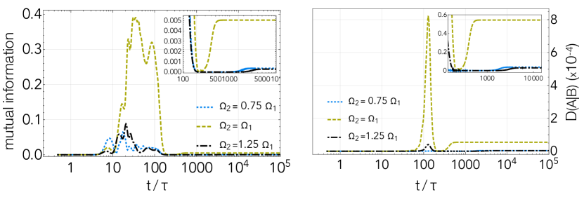
Figure 2: (Left) Mutual information between the two mirrors as a function of time in the cooling regime ($\Delta=\Omega_{1}$). The dotted line refers to the case $\Omega_{2}=0.75\Omega_{1}$, the dashed line refers to the case $\Omega_{2}=\Omega_{1}$ and the dot-dashed one refers to the case $\Omega_{2}=1.25\Omega_{1}$. The box in the right corner zooms on the long time region where is shown the establishment of steady state correlations (Right) Quantum discord $D(A|B)$ in the same cases considered for the mutual information. The box in the right corner shows a zoom of the discord values on the long time region. For these plots the following parameters’ values have been considered: $m{=}150$ ng, $\Omega_{1}/(2\pi){=}1$ MHz, $\gamma/(2\pi){=}1$ Hz ($\gamma_{j}$), $T{=}300$ K, $L{=}25$mm, $\kappa{=}1.34$ MHz, $\lambda{=}1064$ nm, and $P_{1}{=}2$ mW and time is expressed in units of $\tau=2\pi/\Omega_{1}$. These values are consistent with the state of the art experiments and unless otherwise specified these are the ones considered in all the shown results

As shown in fig. 2, the time evolution of the mutual information is characterised by distinct phases. Initially, the two mirrors exhibit no correlation, indicating an uncorrelated state. Following this, a short transient of correlation between the mirrors occurs. Eventually, they return to an uncorrelated state again, only to reach a state of steady-state correlations. Comparing this result with the temperature behaviour reported in fig. 3 can be observed that the rebirth of correlations occurs subsequent to thermalization of the second mirror. The amount of quantumness and, most importantly, the asymmetrical nature (due to the unidirectional coupling) of such correlations can be characterized in terms of quantum Discord [45].

This different type of quantum correlations can be nonzero even in the case of separable states which implies that some bipartite quantum states can show correlations that are incompatible with classical physics. For our system we can adopt the Gaussian quantum Discord [46, 47]. Quantum Gaussian Discord is defined as the difference between mutual information and classical correlations. Classical correlations are defined as the maximum amount of information that one can gain on one subsystem by locally measuring the other subsystem [44] and so, by this definition, quantum Discord is not symmetric with respect to the interchange of the two subsystems. In particular in this case, where the coupling is unidirectional, the Gaussian discord is maximally asymmetrical due to the fact that measuring the first subsystem one cannot recover any information about the second one.

The quantum Discord $D(A|B)$ plotted in fig. 2 refers only to the one relative to the second subsystem conditioned to the first, indeed performing a measure on the second mirror one can recover some information on the first one, but the converse is not true. In fact $D(B|A)$ is identically zero at all times. That is expected due to the unidirectionality of the coupling. Furthermore also for the quantum discord there is a non zero value also in the stationary state.

V Finite temperature gradient

Here we will show that in the cooling regime, due to the effective unidirectional coupling, a temperature gradient is established between the two mechanical modes. In fact in the cooling regime, i.e. $\Delta{=}\Omega_{1}$, the optical field generates extra damping on the mechanical mode. Such optical damping, caused by radiation pressure, depends on both the position $Q$ and the speed with which the mirror changes its position. At $t=0$ the phonons associated to the mechanical oscillator motion are in a thermal equilibrium state. Then, the interaction between the photons and the phonons, as described by the last term in eq. 2, leads to a change of the phonon number which fluctuates due to the coupling to its environment, consisting of a hot phonon bath at temperature $T$. The goal of optomechanical (sideband) cooling is to reduce the amount of such fluctuations thereby cooling it down.

The mean energy of the mirrors is evaluated

$$U_{j}(t)=\frac{\hbar\Omega_{j}}{2}\left(\langle\delta q_{j}^{2}(t)\rangle+\langle\delta p_{j}(t)^{2}\rangle\right)=\hbar\Omega_{j}\left(n^{\text{eff}}_{j}(t)-\frac{1}{2}\right)$$ (20)

with $n^{\text{eff}}_{j}(t)$ obtained by the solution eq. 9 of covariance matrix as $1/2(C_{11}+C_{22}-1)$ for the first mechanical mode and $1/2(C_{55}+C_{66}-1)$ for the second one.

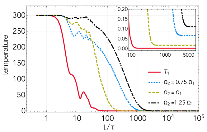
Figure 3: Temperatures of mechanical modes, as defined in eq. 21, as a function of time. The solid line refers to the temperature of the first mirror, the dotted one refers to the temperature of the second mirror in the case $\Omega_{2}=0.75\Omega_{1}$, the dashed line represents the the temperature of the second mirror in the case $\Omega_{2}=\Omega_{1}$, while the dot-dashed one represents the temperature of the second mirror in the case $\Omega_{2}=1.25\Omega_{1}$

The effective temperature of the movable mirrors are then given by

$$T^{\text{eff}}_{j}(t)=\frac{\hbar\Omega_{j}}{k_{B}\ln{(1+1/n^{\text{eff}}_{j}(t)})}$$ (21)

When the two mirrors have the same frequency, i.e. $\Omega_{2}=\Omega_{1}$ (fig. 3), the steady state is characterised by a higher temperature of the second mirror with respect to the first one. This is a consequence of the unidirectionality of the coupling. Indeed, as shown in appendix, such temperature gradient is absent in the bidirectional case.

To further investigate the properties of this temperature gradient, the temperatures of the second mirror were evaluated varying its frequency. Due to the mismatch between the optical detuning and the frequency of the mechanical mode in the second optomechanical system, which corresponds to a variation in the cooling efficiency, the time at which the second mirror reaches a steady temperature value, $t_{s}$, increases as shown in fig. 4 as long as the frequency is moving apart from the resonant case $\Omega_{2}=\Omega_{1}$

It can be seen in fig. 5 that for different values of $\Omega_{2}$, varying the detuning between the pump and the first cavity, one can always tune it in such a way that it creates a temperature gradient between the mirrors. The stationary correlations between the two mirrors, evaluated as the mutual information in the stationary regime, shows a peak in correspondence to the minima of the second mirror temperatures.

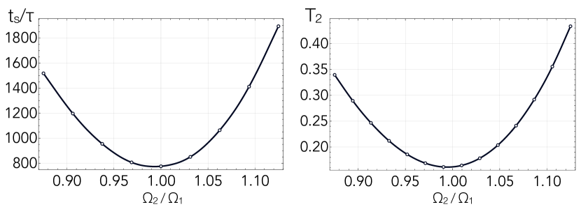
Figure 4: (Left) Time at which the second mechanical mode reaches the stationary state as a function of its frequency (Right) Temperature of the second mechanical mode in the stationary regime as a function of its frequency

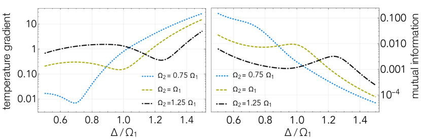
Figure 5: (Left) Temperature gradients of mechanical modes $T^{\text{eff}}_{2}-T^{\text{eff}}_{1}$, where $T^{\text{eff}}_{j}$ is defined as in eq. 21, in the stationary limit for different values of $\Omega_{2}$. In particular, the curves refer to the cases $\Omega_{2}=0.75\Omega_{1}$, $\Omega_{2}=\Omega_{1}$ and $\Omega_{2}=1.25\Omega_{1}$. (Right) Mutual information between the two mechanical modes in the stationary limit for the same values of $\Omega_{2}$

VI The steady state and the power spectra

One of the experimentally accessible quantity for the optomechanical systems is the power spectrum of the cavity output field which allows to reconstruct the spectrum (and so the dynamics and the temperature) of the mechanical mirror [48]. We now show how in this cascaded configuration, the spectrum in output from the last cavity contains informations about the two mirrors and allows to reconstruct their dynamics. In order to evaluate the spectra of the cavity output and the two individual mirrors, it’s necessary to evaluate the stationary state of the system. As shown in the previous sections, the linearized equations for the fluctuations eq. 8 can be solved in the frequency domain. The correlation functions eq. 3 become

$$\langle\hat{a}^{\text{in}}(\omega)\hat{a}^{\text{in}\dagger}(\omega^{\prime})\rangle=\delta(\omega+\omega^{\prime})$$ (22a)

$$\langle\{\hat{\xi}_{j}(\omega),\xi_{j}(\omega^{\prime})\}\rangle=2\gamma\coth\left(\frac{\hbar\Omega_{j}}{2k_{B}T}\right)\delta(\omega+\omega^{\prime}),$$ (22b)

while the equations for the fluctuations of cavity field modes are eq. 13 and the equations for the positions of the mirrors become

$$\delta\hat{q}_{j}(\omega)=\chi_{j}(\omega)\left(G_{j}\delta\hat{a}_{j}^{\dagger}(\omega)+G^{*}_{j}\delta\hat{a}_{j}(\omega)+\xi_{j}(\omega)\right)$$ (23)

where we have introduced the natural susceptibilities of the mechanical modes

$$\chi_{j}(\omega)=\frac{\Omega_{j}}{\Omega_{j}^{2}-\omega^{2}-i\omega\gamma}$$ (24)

The mirror’s position fluctuations can be expressed in terms of effective susceptibilities and noise operators:

$$\delta\hat{q}_{1}(\omega)= \chi^{\text{eff}}_{1}(\omega)\xi_{1}(\omega)$$ (25a)

$$\delta\hat{q}_{2}(\omega)= \chi^{\text{eff}}_{2}(\omega)\xi^{\text{eff}}_{2}(\omega)$$ (25b)

with

$$\chi_{j}^{\text{eff}}(\omega)=\frac{\chi_{j}(\omega)}{1-i|G_{j}|^{2}\chi_{j}(\omega)(\chi_{a_{j}}(\omega)-\chi_{a_{j}}^{*}(\text{-}{\omega}))}$$ (26a)

$$\xi^{\text{eff}}_{2}(\omega)=\xi_{2}(\omega)-i\kappa\chi^{\text{eff}}_{1}(\omega)\xi_{1}(\omega)\Lambda(\omega)$$ (26b)

Note that the effective susceptibility of the mechanical oscillators $\chi_{j}^{\text{eff}}(\omega)$ are modified by the radiation pressure [3]. Furthermore, in the second of eq. 25, the effective noise seen by the second mirror, modified by the presence of the first, is made explicit. It is now clear how the position fluctuations of the first ($\delta\hat{q}_{1}$) of the two mechanical modes depends only on its local thermal bath, while the second one ($\delta\hat{q}_{2}$) depends also on the thermal bath of the first via the optical field.

In the same way, for the cavity field fluctuation we have

$$\delta\hat{a}_{1}(\omega) =iG_{1}\chi_{a_{1}}(\omega)\chi^{\text{eff}}_{1}(\omega)\xi_{1}(\omega)$$ (27a)

$$\delta\hat{a}_{2}(\omega) =iG_{2}\chi_{a_{2}}(\omega)\chi^{\text{eff}}_{2}(\omega)\xi^{\text{eff}}_{2}(\omega)-iG_{1}\kappa\chi_{a_{1}}(\omega)\chi_{a_{2}}(\omega)\chi^{\text{eff}}_{1}(\omega)\xi_{1}(\omega)$$ (27b)

Power Spectra

From eqs. 25 and 27, thanks to eq. 22, it is possible to evaluate the position spectrum of the two mirrors defined by

$$S^{q}_{j}(\omega)=\frac{1}{\sqrt{2\pi}}\int_{-\infty}^{+\infty}d\Omega e^{-i(\omega+\Omega)t}\langle\delta\hat{q}_{j}(\omega)\delta\hat{q}_{j}(\Omega)\rangle$$ (28)

obtaining

$$S^{q}_{1}(\omega){=} \gamma(2\bar{n}_{1}{+}1)|\chi_{1}^{\text{eff}}(\omega)|^{2}$$ (29a)

$$S^{q}_{2}(\omega){=} \gamma(2\bar{n}_{2}{+}1)|\chi_{2}^{\text{eff}}(\omega)|^{2}{-}\kappa^{2}S^{q}_{1}(\omega)|\chi_{2}^{\text{eff}}(\omega)|^{2}|\Lambda(\omega)|^{2}$$ (29b)

from which one can obtain the variances $\langle\delta\hat{q}_{j}^{2}\rangle$ trough

$$\langle\delta\hat{q}_{j}^{2}\rangle=\int_{-\infty}^{+\infty}\frac{d\omega}{2\pi}S^{q}_{j}(\omega)$$ (30)

We are also interested to the output power spectral density that would be detected in an homodyne detection of the output fluctuations $\delta x^{\text{out}}{=}1/\sqrt{2}(\delta\hat{a}^{\text{out}}+\delta\hat{a}^{\dagger\text{out}})$ where

$$\delta\hat{a}^{\text{out}}(\omega)=\hat{a}^{\text{in}}(\omega)-\sqrt{\kappa}\delta\hat{a}_{1}(\omega)-\sqrt{\kappa}\delta\hat{a}_{2}(\omega)$$ (31)

The spectrum of such fluctuations can be obtained as

$$P^{\text{out}}(\omega)=\frac{1}{\sqrt{2\pi}}\int_{-\infty}^{+\infty}d\Omega e^{-i(\omega+\Omega)t}\braket{x^{\text{out}}(\omega)x^{\text{out}}(\Omega)}$$ (32)

Using eq. 22 in the frequency domain one finds

$$P^{\text{out}}(\omega)\sim\sum_{j=1}^{2}K_{j}(\omega)S^{q}_{j}(\omega)$$ (33)

with $K_{j}(\omega)=\kappa|{G_{j}\chi_{a_{j}}(\omega){-}G_{j}^{*}\chi_{a_{j}}^{*}(\text{-}{\omega})}|^{2}/2$. From eq. 33, it follows, as shown in fig. 6, that the output field from the second cavity contains information on the power spectra of both mechanical modes as it simply proportional to the sum of the two mechanical power spectra. A similar result was obtained, for a single optomechanical system, in [48]. Consequently, the peaks observed in the cavity’s output spectrum reflect those of the individual mirrors’ spectra. Hence, one can infer the power spectrum of each individual mirror by fitting the peaks of the spectrum, given that the power spectrum of an individual optomechanical mirror is well approximated by a Lorentzian curve [2].

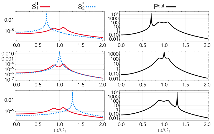
Figure 6: (Left) Mirror’s Spectra - In this figure we plot the power spectrum eq. 29 of the first mechanical mode and of the second one for three different frequencies, from top to bottom, $\Omega_{2}=\Omega_{1}/2$, $\Omega_{2}=\Omega_{1}$ and $\Omega_{2}=3\Omega_{1}/2$. (Right) Output Spectra - Spectrum of the output field from the second cavity. In this case $P=10^{-2}mW$

The appearance of two peaks in the power spectra of the first mirror, as depicted in fig. 6, is contingent on the selected value for the first cavity’s pump power. Specifically, these dual peaks manifest at a particular power pump value and progressively move farther apart as the power value increases.

VII Self-induced oscillations and multistability

Up until this point, our analysis has primarily focused on stable states by employing specific parameter values. However, we will now delve into the nonlinear regime for the average values and demonstrate how to identify stable states by tuning the system’s parameters. As the optomechanical coupling becomes stronger and damping becomes weaker, the system’s nonlinearities become significant and cannot be neglected any longer. In this regime, the system exhibits instabilities, leading the mirror to enter a state of what is known as ”self-sustained oscillations”. In the following, we will explore these nonlinear dynamics and outline the conditions required to achieve stable states amidst the presence of these oscillations[49, 50]. In this regime the mean position of the mirrors can be written as $Q_{j}(t)=\bar{Q}_{j}{+}\alpha_{j}cos(\Omega_{j}t)$. Putting this into eq. 7, the exact solutions for the cavity modes amplitude $A_{j}$, in the long time limit, can be written as

$$A_{1}(t)= \exp\left[ig_{1}\alpha_{1}\frac{\sin(\Omega_{1}t)}{\Omega_{1}}\right]\sum_{n}A_{1}^{n}e^{i\Omega_{1}nt}$$ (34a)

$$A_{2}(t)= \exp\left[ig_{2}\alpha_{2}\frac{\sin(\Omega_{2}t)}{\Omega_{2}}\right]\sum_{n,m,l}A_{2}^{nml}e^{i(\Omega_{1}(n+l)+\Omega_{2}m)t}$$ (34b)

with

$$A_{1}^{n}=J_{n}\left(\frac{-g_{1}\alpha_{1}}{\Omega_{1}}\right)\chi_{a_{1}}(-\Omega_{1}n)E_{1}$$ (35a)

$$A_{2}^{nml}=-\kappa\;J_{n}\left(-\frac{g_{1}\alpha_{1}}{\Omega_{1}}\right)\;J_{m}\left(-\frac{g_{2}\alpha_{2}}{\Omega_{2}}\right)J_{l}\left(\frac{g_{1}\alpha_{1}}{\Omega_{1}}\right)\chi_{a_{2}}(-\Omega_{1}(n+l)-\Omega_{2}m)\;E_{1}$$ (35b)

where $J_{n}(x)$ is the Bessel function of first kind and $\chi_{a_{j}}$ are the susceptibilities defined in eq. 14. The stable states of the system are those for which the total time-averaged force vanishes and the power due to the radiation pressure $P_{rad_{j}}=G\langle|A_{j}|^{2}\dot{Q}_{j}\rangle$ equals the power dissipated $P_{fric}=\gamma\langle\dot{Q}^{2}_{j}\rangle$. By plotting the ratio $P_{rad}/P_{fric}$ for the two subsystems as a function of $A_{j}$ and detuning $\Delta$, we obtain diagrams that illustrate the parameter regions corresponding to stable states. These diagrams provide valuable insights into the values of $A_{j}$ and $\Delta$ where the system exhibits stability.

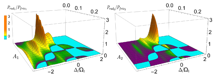
Figure 7: (Left) Stability plot for the first mechanical oscillator. It shows the ratio between the power due to radiation pressure and the power dissipated as a function of the amplitude of oscillation and the detuning between the pump and the cavity[50]. (Right) Stability Graph for the second mechanical oscillator, it shows the ratio between the power due to radiation pressure and the power dissipated as a function of the amplitude of oscillation and the detuning between the pump and the cavity. In both the plots, the stable states are those for which the power due to the radiation pressure $P_{rad_{j}}=G\langle|A_{j}|^{2}\dot{Q}_{j}\rangle$ equals the power dissipated $P_{fric}=\gamma\langle\dot{Q}^{2}_{j}\rangle$

Multistability - A characteristic feature of optomechanical systems is that, in the regime in which $A_{j}=0$, they exhibit multistability. A given intensity of the light pumped in the cavity can lead to different steady states of both cavity photon number and mechanical position [2, 51]. From eq. 7, taking the stationary limit, we can find the equations for the average number of photons in the two cavities $N_{j}$ i.e.

$$\dfrac{g^{4}_{1}}{\Omega^{2}_{1}}N^{3}_{1}-\dfrac{2\Delta g^{2}_{1}}{\Omega_{1}}N^{2}_{1}+\left(\Delta^{2}+\dfrac{\kappa^{2}}{2}\right)N_{1}-E^{2}_{1}=0$$ (36a)

$$\dfrac{g^{4}_{2}}{\Omega^{2}_{2}}N^{3}_{2}-\dfrac{2\Delta g^{2}_{2}}{\Omega_{2}}N^{2}_{2}+\left(\Delta^{2}+\dfrac{\kappa^{2}}{2}\right)N_{2}-\kappa^{2}N_{1}=0$$ (36b)

and once found these, we can find the average cantilever positions as

$$Q_{j}=\dfrac{g_{j}}{\Omega_{j}}N_{j}$$ (37)

We note that the first of eq. 36 has three roots, but, as shown also in [51], only two of these solutions are stable solutions, specifically the lower and the higher ones while the middle one is unstable and can’t be observed experimentally. Regarding the equation for the second cavity a richer behaviour is obtained, as shown in fig. 8.

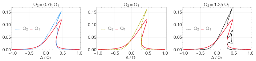
Figure 8: Steady-state position of the cantilevers as a function of detuning for $\Omega_{2}{=}3/4\Omega_{1}$(left), $\Omega_{2}{=}\Omega_{1}$(center) and $\Omega_{2}{=}5/4\Omega_{1}$(right). As known in literature [2, 51], the positions of mirrors show multistability. In a single optomechanical system the mechanical position have three stable solutions, but due to the unidirectional coupling the second one shows three or more stable solutions depending on the detuning between the two mirror’s frequencies

VIII Conclusion

In summary, this study has provided a comprehensive characterization of the dynamics of two optomechanical systems indirectly coupled via a chiral waveguide in a cascaded configuration. In the weak coupling regime, we employed an adiabatic elimination technique to derive effective equations governing the mirror dynamics.

By examining the evolution of correlations between the two mechanical modes, we quantified their mutual information and quantum discord over time. Remarkably, our results demonstrate that these correlations persist even in the stationary state, indicating a non-zero value of steady correlations. Furthermore, we investigated the steady-state temperatures of both mirrors for different values of $\Omega_{2}$ and various $\Delta$ parameters. Our findings revealed the existence of a finite temperature difference between the two mirrors when employing this indirect effective coupling approach. This suggests the exciting possibility of engineering a temperature gradient between the mechanical modes using such a setup. Additionally, we analysed the power spectra of the two mechanical modes and the output spectrum of the second cavity. Remarkably, our study shows that by measuring the latter, it becomes feasible to reconstruct the spectra of the mirrors accurately. To ensure the stability of the mirror dynamics, we explored the regions of stability as a function of the first cavity pump. Moreover, we delved into the potential existence of multiple steady states for both cavity photon number and mechanical position concerning a specific intensity of light pumped into the first cavity.

The findings regarding correlations, temperature gradients, spectrum reconstruction, stability regions, and multiple steady states open up new possibilities for controlling and manipulating these complex systems for various applications.

Appendix A

Two modes mutual information and quantum discord

As known by [44] given a two-mode Gaussian state covariance matrix

$$\mathbf{C}=\begin{pmatrix}\mathbf{A}&\mathbf{D}\\ \mathbf{D}^{T}&\mathbf{B}\\ \end{pmatrix},$$ (38)

where $\mathbf{A}$, $\mathbf{B}$ and $\mathbf{D}$ are $2\times 2$ matrices one can define four local symplectic invariants, $I_{1}=det(\mathbf{A})$, $I_{2}=det(\mathbf{B})$, $I_{3}=det(\mathbf{D})$, $I_{4}=det(\mathbf{C})$ and its symplectic eigenvalues

$$d_{\pm}=\sqrt{\dfrac{I_{\Delta}\pm\sqrt{I_{\Delta}^{2}-4I_{4}}}{2}}$$ (39)

where $I_{\Delta}=I_{1}+I_{2}+2I_{3}$.
Mutual information, defined for two quantum systems A and B as

$$\mathcal{I}(AB)=S(\rho_{A})+S(\rho_{B})-S(\rho_{AB})$$ (40)

(where $S(\rho)$ refers to Von Neumann entropy) can be evaluated, in the case of continous variables gaussian states, in terms of those symplectic invariants as

$$\mathcal{I}(AB)=f(\sqrt{I_{1}})+f(\sqrt{I_{2}})-f(d_{+})-f(d_{-})$$ (41)

with

$$f(x)=\left(x+\dfrac{1}{2}\right)log\left(x+\dfrac{1}{2}\right)-\left(x-\dfrac{1}{2}\right)log\left(x-\dfrac{1}{2}\right).$$ (42)

Mutual information quantifies the correlations between two quantum systems. Quantum discord, interpreted as the amount on quantumness of these correlations, is then defined as

$$\mathcal{D}(A|B)=\mathcal{I}(AB)-\mathcal{C}(A|B)$$ (43)

where

$$\mathcal{C}(A|B)=\max_{\{E_{a}\}}\left[S(\rho_{A})-\sum_{a}p_{a}S\left(\frac{Tr_{B}[\rho_{AB}E_{a}]}{p_{a}}\right)\right]$$ (44)

is the total amount of classical correlations and $\sum_{a}E_{a}=\mathbf{1}$ is a positive operator value measurement (POVM).
In terms of symplectic invariants of covariance matrix, quantum discord can be evaluated as

$$\mathcal{D}(A|B)=f(\sqrt{I_{2}})+f(d_{+})+f(d_{-})+f(\sqrt{W}),$$ (45)

where

$$W=\begin{cases}\left[\frac{2|I_{3}|+\sqrt{4I^{2}_{3}+(4I_{2}-1)(4I_{4}-1)}}{(4I_{2}-1)}\right]^{2}\text{ if }\frac{4(I_{1}I_{2}-I_{4})^{2}}{(I_{1}+4I_{4})(1+4I_{2})I^{2}_{3}}\leq 1,\\ \\ \frac{I_{1}I_{2}+I_{4}-I^{2}_{3}-\sqrt{(I_{1}I_{2}+I_{4}-I^{2}_{3})^{2}-4I_{1}I_{2}I_{4}}}{2I_{2}}\text{ otherwise.}\end{cases}$$ (46)

Appendix B

Bidirectional case

In order to consider the most general case in which the two subsystems are coupled through a bidirectional (non chiral) waveguide it’s necessary to introduce two vacuum input noise operators, $\hat{a}^{in}_{R}$ and $\hat{a}^{in}_{L}$, one for each of the direction of propagation in the waveguide, with autocorrelation functions:

$$\braket{\hat{a}^{in}_{i}(t)\hat{a}^{in\dagger}_{j}(t^{\prime})}=\delta_{ij}\delta(t-t^{\prime})\text{\quad with\quad}i,j=R,L$$ (47)

and the same Brownian noise operators $\hat{\xi}_{j}$ defined in section II.
Once defined these new operators, one can straightforwardly follow the procedure described in the previous sections and find the new set of non linear differential equations for the mean values

$$\frac{dQ_{j}(t)}{dt}=\Omega_{j}P_{j}(t)$$ (48a)

$$\frac{dP_{j}(t)}{dt}=-\Omega_{j}Q_{j}(t)-\gamma_{j}P_{j}(t)+|G_{j}(t)|^{2}/g_{j}$$ (48b)

$$\frac{dA_{1}(t)}{dt}=-\frac{\kappa}{2}A_{1}(t)-i\Delta_{1}(t)A_{1}(t)-\kappa A_{2}(t)+E_{1}$$ (48c)

$$\frac{dA_{2}(t)}{dt}=-\frac{\kappa}{2}A_{2}(t)-i\Delta_{2}(t)A_{2}(t)-\kappa A_{1}(t)+E_{2}$$ (48d)

and for the fluctuations one can again find a Lyapunov equation that the covariance matrix $\mathbf{C}$ of the system must obey

$$\frac{d\mathbf{C}(t)}{dt}=\mathbf{S}(t)\mathbf{C}(t)+\mathbf{C}(t)\mathbf{S}(t){+}\mathbf{N}$$ (49)

in which the drift ($\mathbf{S}$) and diffusion ($\mathbf{N}$) matrices now become (cfr. eq. 9)

$$\mathbf{S}=\begin{pmatrix}\mathbf{S}_{1}&\mathbf{S}_{12}\\ \mathbf{S}_{12}&\mathbf{S}_{2}\end{pmatrix}\qquad\text{and}\qquad\mathbf{N}=\begin{pmatrix}\mathbf{N}_{1}&\mathbf{N}_{12}\\ \mathbf{N}_{12}&\mathbf{N}_{2}\end{pmatrix}$$ (50)

with

$$\mathbf{S}_{j}{=}\begin{pmatrix}0&\Omega_{j}&0&0\\ -\Omega_{j}&-\gamma&\text{Re}(G_{j})&\text{Im}(G_{j})\\ -\text{Im}(G_{j})&0&-\kappa&\Delta_{j}\\ \text{Re}(G_{j})&0&-\Delta_{j}&-\kappa\end{pmatrix}\;\;\mathbf{S}_{12}{=}\begin{pmatrix}0&0&0&0\\ 0&0&0&0\\ 0&0&-\kappa&0\\ 0&0&0&-\kappa\end{pmatrix}$$

and

$$\mathbf{N}_{j}{=}\begin{pmatrix}0&0&0&0\\ 0&\gamma(2\bar{n}_{j}+1)&0&0\\ 0&0&2\kappa&0\\ 0&0&0&2\kappa\\ \end{pmatrix}\;\;\mathbf{N}_{12}{=}\begin{pmatrix}0&0&0&0\\ 0&0&0&0\\ 0&0&2\kappa&0\\ 0&0&0&2\kappa\end{pmatrix}$$

It’s possible now to calculate the temperature as defined in eq. 21 and, as shown in fig. 9, in the case in which the two optomechanical systems are pumped (i.e. $E_{2}=E_{1}=E$) it can be seen that no gradient of temperature is established between the two mirrors.

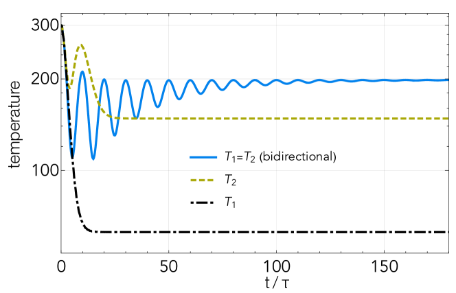
Figure 9: In this figure is reported the temperature of the two mirrors in the unidirectional (dashed and dot-dashed lines) and bidirectional (solid line) as a function of time, for $E_{1}=E_{2}=E$ and $\gamma=2\pi\cdot 10^{4}$. In order to compare systems with constant total decay rate in the unidirectional case the decay rates were fixed with values $\kappa_{R}=\kappa$ and $\kappa_{L}=0$, while in the bidirectional case $\kappa_{R}=\kappa_{L}=\kappa/2$. In the first case one can see that a temperature gradient is established while in the latter is not present anymore.

Appendix C

Effective Lorenzian peak

The expression for the spectra in eq. 29 can be rearranged, expliciting the expressions of $\chi_{\text{eff}_{j}}$, $\chi_{j}$ and $\chi_{a_{j}}$ in the form that, in the limit of $\omega_{j}\simeq\Omega_{j}$, is a Lorenzian curve. Indeed if we write $\chi_{\text{eff}_{j}}$ expliciting the susceptibilities we obtain

$$\chi_{j}^{\text{eff}}(\omega)=\frac{\chi_{j}(\omega)}{1-i|G_{j}|^{2}\chi_{j}(\omega)(\chi_{a_{j}}(\omega)-\chi_{a_{j}}^{*}(\text{-}{\omega}))}=$$ (51)

$$=\frac{\Omega_{j}}{\Omega_{j}-\omega^{2}-i\gamma\omega-i|G_{j}|^{2}\Omega_{j}\left(\frac{1}{\frac{\kappa}{2}-i(\omega-\Delta_{j})}-\frac{1}{\frac{\kappa}{2}-i(\omega+\Delta_{j})}\right)}.$$

If we define $\tilde{\Omega}_{j}(\omega)$ and $\tilde{\gamma}_{j}(\omega)$ as

$$\tilde{\Omega}_{j}(\omega)=\sqrt{\Omega^{2}_{j}-\frac{|G_{j}|^{2}2\Delta_{j}\Omega_{j}(\frac{\kappa^{2}}{4}+\Delta^{2}_{j}-\omega^{2})}{(\frac{\kappa^{2}}{4}+(\omega-\Delta_{j})^{2})(\frac{\kappa^{2}}{4}+(\omega+\Delta_{j})^{2})}}$$ (52)

$$\tilde{\gamma}_{j}(\omega)=\gamma+\frac{|G_{j}|^{2}2\kappa\Delta_{j}\Omega_{j}}{(\frac{\kappa^{2}}{4}+(\omega-\Delta_{j})^{2})(\frac{\kappa^{2}}{4}+(\omega+\Delta_{j})^{2})}$$

we can rewrite eq. 51 as

$$\chi^{\text{eff}}_{j}(\omega)=\frac{\Omega_{j}}{\tilde{\Omega}^{2}_{j}(\omega)-\omega^{2}-i\tilde{\gamma}_{j}(\omega)\omega}$$ (53)

which in the neighborhood of $\omega=\Omega_{j}$ can be approximated by

$$\chi^{\text{eff}}_{j}(\omega)=\frac{\Omega_{j}}{\tilde{\Omega}^{2}_{j}(\Omega_{j})-\omega^{2}-i\tilde{\gamma}_{j}(\Omega_{j})\omega}$$ (54)

Being proportional to the squared modulus of $\chi^{\text{eff}}_{j}$, the spectra will have the shape of a Lorenzian curve as shown in fig. 10.

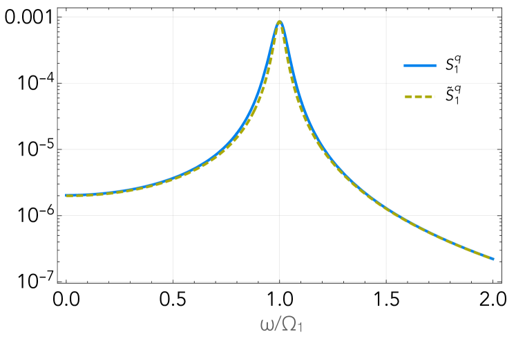
Figure 10: Spectrum of the first mirror plotted using the exact expression (solid line) and with the one obtained approximating the spectrum as a lorenzian (dashed line)

References

References

- [1] Aspelmeyer M, Gröblacher S, Hammerer K and Kiesel N 2010 Journal of the Optical Society of America B 27 A189 ISSN 0740-3224
- [2] Bowen W P 2020 Quantum Optomechanics / Warwick P. Bowen, Gerard J. Milburn. (Boca Raton. FL: CRC Press, Taylor & Francis Group) ISBN 978-0-367-57519-9
- [3] Genes C, Vitali D, Tombesi P, Gigan S and Aspelmeyer M 2008 Physical Review A 77 033804
- [4] Gigan S, Böhm H R, Paternostro M, Blaser F, Langer G, Hertzberg J B, Schwab K C, Bäuerle D, Aspelmeyer M and Zeilinger A 2006 Nature 444 67–70 ISSN 14764687
- [5] Marquardt F, Chen J P, Clerk A A and Girvin S M 2007 Physical Review Letters 99 093902 ISSN 00319007
- [6] Marquardt F, Clerk A A and Girvin S M 2008 Quantum theory of optomechanical cooling Journal of Modern Optics vol 55 pp 3329–3338 ISSN 09500340
- [7] Yang J Y, Wang D Y, Bai C H, Guan S Y, Gao X Y, Zhu A D and Wang H F 2019 Optics Express 27 22855–22867 ISSN 1094-4087
- [8] Pham V N T, Hoang C M and Vy N D 2021 Journal of Modern Optics 68 63–71 (Preprint eprint https://doi.org/10.1080/09500340.2021.1875073) URL https://doi.org/10.1080/09500340.2021.1875073
- [9] Delić U, Reisenbauer M, Dare K, Grass D, Vuletić V, Kiesel N and Aspelmeyer M 2020 Science 367 892–895 (Preprint eprint https://www.science.org/doi/pdf/10.1126/science.aba3993) URL https://www.science.org/doi/abs/10.1126/science.aba3993
- [10] Lecocq F, Clark J B, Simmonds R W, Aumentado J and Teufel J D 2015 Physical Review X 5 041037
- [11] Pirkkalainen J M, Damskägg E, Brandt M, Massel F and Sillanpää M A 2015 Physical Review Letters 115 243601
- [12] Magrini L, Camarena-Chávez V A, Bach C, Johnson A and Aspelmeyer M 2022 Phys. Rev. Lett. 129(5) 053601 URL https://link.aps.org/doi/10.1103/PhysRevLett.129.053601
- [13] Palomaki T A, Teufel J D, Simmonds R W and Lehnert K W 2013 Science 342 710–713
- [14] Riedinger R, Hong S, Norte R A, Slater J A, Shang J, Krause A G, Anant V, Aspelmeyer M and Gröblacher S 2016 Nature 530 313–316 ISSN 1476-4687
- [15] Gut C, Winkler K, Hoelscher-Obermaier J, Hofer S G, Nia R M, Walk N, Steffens A, Eisert J, Wieczorek W, Slater J A, Aspelmeyer M and Hammerer K 2020 Physical Review Research 2 033244
- [16] Hong S, Riedinger R, Marinković I, Wallucks A, Hofer S G, Norte R A, Aspelmeyer M and Gröblacher S 2017 Science 358 203–206 (Preprint eprint https://www.science.org/doi/pdf/10.1126/science.aan7939) URL https://www.science.org/doi/abs/10.1126/science.aan7939
- [17] Bhattacharya M and Meystre P 2008 Physical Review A 78 041801
- [18] Xuereb A, Genes C, Pupillo G, Paternostro M and Dantan A 2014 Physical Review Letters 112 133604
- [19] Xuereb A, Genes C and Dantan A 2012 Physical Review Letters 109 223601
- [20] Weaver M J, Buters F, Luna F, Eerkens H, Heeck K, de Man S and Bouwmeester D 2017 Nature Communications 8 824 ISSN 2041-1723
- [21] Piergentili P, Li W, Natali R, Malossi N, Vitali D and Giuseppe G D 2021 New Journal of Physics 23 073013 ISSN 1367-2630
- [22] Peano V, Brendel C, Schmidt M and Marquardt F 2015 Physical Review X 5 031011
- [23] Gan J H, Xiong H, Si L G, Lü X Y and Wu Y 2016 Optics Letters 41 2676–2679 ISSN 1539-4794
- [24] Heinrich G, Ludwig M, Qian J, Kubala B and Marquardt F 2011 Physical Review Letters 107 043603
- [25] Gil-Santos E, Labousse M, Baker C, Goetschy A, Hease W, Gomez C, Lemaître A, Leo G, Ciuti C and Favero I 2017 Physical Review Letters 118 063605
- [26] Pichler H, Ramos T, Daley A J and Zoller P 2015 Physical Review A 91 042116
- [27] Giovannetti V and Palma G M 2012 Journal of Physics B: Atomic, Molecular and Optical Physics 45 154003 ISSN 0953-4075
- [28] Giovannetti V and Palma G M 2012 Physical Review Letters 108 040401
- [29] Ramos T, Pichler H, Daley A J and Zoller P 2014 Physical Review Letters 113 237203
- [30] Cusumano S, Mari A and Giovannetti V 2018 Physical Review A 97 053811
- [31] Karg T M, Gouraud B, Treutlein P and Hammerer K 2019 Physical Review A 99 063829
- [32] Farace A, Ciccarello F, Fazio R and Giovannetti V 2014 Phys. Rev. A 89(2) 022335 URL https://link.aps.org/doi/10.1103/PhysRevA.89.022335
- [33] Li T, Bao T Y, Zhang Y L, Zou C L, Zou X B and Guo G C 2016 Optics Express 24 12336–12348 ISSN 1094-4087 publisher: Optical Society of America URL https://www.osapublishing.org/oe/abstract.cfm?uri=oe-24-11-12336
- [34] Li J, Zhou Z H, Wan S, Zhang Y L, Shen Z, Li M, Zou C L, Guo G C and Dong C H 2022 Phys. Rev. Lett. 129(6) 063605 URL https://link.aps.org/doi/10.1103/PhysRevLett.129.063605
- [35] Xuereb A, Barzanjeh S and Aquilina M 2018 Routing thermal noise through quantum networks p 59
- [36] Law C K 1995 Physical Review A 51 2537–2541 ISSN 10502947
- [37] Genes C, Mari A, Vitali D and Tombesi P 2009 Chapter 2 Quantum Effects in Optomechanical Systems
- [38] Giovannetti V and Vitali D 2001 Physical Review A - Atomic, Molecular, and Optical Physics 63 1–8 ISSN 10502947
- [39] Gardiner C W and Parkins A S 1994 Physical Review A 50 1792–1806 ISSN 10502947
- [40] Gardiner C W and Zoller P Quantum Noise
- [41] Gardiner C W and Collett M J 1985 Physical Review A 31 3761–3774 ISSN 10502947
- [42] Wilson-Rae I, Nooshi N, Zwerger W and Kippenberg T J 2007 Physical Review Letters 99 093901 ISSN 00319007
- [43] Serafini G, Zippilli S and Marzoli I 2020 Phys. Rev. A 102(5) 053502 URL https://link.aps.org/doi/10.1103/PhysRevA.102.053502
- [44] Olivares S 2012 European Physical Journal: Special Topics 203 3–24 ISSN 19516355
- [45] Ollivier H and Zurek W H 2001 Phys. Rev. Lett. 88(1) 017901 URL https://link.aps.org/doi/10.1103/PhysRevLett.88.017901
- [46] Adesso G and Datta A 2010 Phys. Rev. Lett. 105(3) 030501 URL https://link.aps.org/doi/10.1103/PhysRevLett.105.030501
- [47] Giorda P and Paris M G A 2010 Phys. Rev. Lett. 105(2) 020503 URL https://link.aps.org/doi/10.1103/PhysRevLett.105.020503
- [48] Paternostro M, Gigan S, Kim M S, Blaser F, Böhm H R and Aspelmeyer M 2006 New Journal of Physics 8 107–107 ISSN 13672630
- [49] Ludwig M, Kubala B and Marquardt F 2008 New Journal of Physics 10 ISSN 13672630
- [50] Marquardt F, Harris J G E and Girvin S M 2006 Physical Review Letters 96 103901
- [51] Sarma B and Sarma A K 2016 J. Opt. Soc. Am. B 33 1335–1340 URL https://opg.optica.org/josab/abstract.cfm?URI=josab-33-7-1335