Cosmological Flow of Primordial Correlators

Abstract

Correlation functions of primordial density fluctuations provide an exciting probe of the physics governing the earliest moments of our Universe. However, the standard approach to compute them is technically challenging. Theoretical predictions are therefore available only in restricted classes of theories. In this Letter, we present a complete method to systematically compute tree-level inflationary correlators. This method is based on following the time evolution of equal-time correlators and it accurately captures all physical effects in any theory. These theories are conveniently formulated at the level of inflationary fluctuations, and can feature any number of degrees of freedom with arbitrary dispersion relations and masses, coupled through any type of time-dependent interactions. We demonstrate the power of this approach by exploring the properties of the cosmological collider signal, a discovery channel for new high-energy physics, in theories with strong mixing and in the presence of features. This work lays the foundation for a universal program to assist our theoretical understanding of inflationary physics and generate theoretical data for an unbiased interpretation of upcoming cosmological observations.

Introduction.

Cosmology is about understanding time. Indeed, the physics governing the universe is deciphered through the time evolution of density perturbations, from the beginning of the Hot Big Bang to the late-time galaxy distribution. Remarkably, it is believed that these perturbations have emerged from quantum zero-point fluctuations during a period of accelerated expansion Guth (1981); Linde (1982); Albrecht and Steinhardt (1982), i.e. cosmic inflation, providing the initial seeds for the subsequent evolution of cosmological structures Mukhanov and Chibisov (1981); Starobinsky (1982); Hawking (1982); Guth and Pi (1982); Bardeen et al. (1983). Tracking down the cosmological flow of inflationary fluctuations thus connects the quantum laws of physics at a fundamental level to the largest observable scales.

Yet, the correct theory of inflation remains unknown, and a central challenge is to decode it through the study of inflationary correlators, namely spatial correlation functions of the curvature perturbation field $\zeta(\bm{x},t)$. On large scales, current data have already well constrained the physics of inflation, especially at the linear level Akrami et al. (2020a). However, much information—e.g. the number of fields active during inflation, together with their mass spectra, spins, sound speeds, and how they interact—is encoded in non-linearities (see e.g. Achúcarro et al. (2022) for a recent review), of which the primary observable is the three-point correlator (bispectrum) (see Akrami et al. (2020b) for current bounds).

Computing equal-time correlators given an inflationary theory is a well-established procedure Weinberg (2005a). From first principles, calculations can be carried to arbitrary orders of perturbation theory. However, this program hides a daunting complexity: perturbation theory becomes intractable for realistic situations. The root of this difficulty resides in the challenge to track the detailed time evolution of the physics in the bulk of spacetime. Consequently, for technical reasons, most of the theoretical predictions have been derived under stringent assumptions, such as assuming weak mixing, perfect (or almost) scale invariance, large hierarchy of masses and couplings, and considering single-exchange diagrams Achúcarro et al. (2022). Therefore, they do not cover the vast panorama of inflationary scenarios Baumann and McAllister (2015). This can completely bias our interpretation of data and reveals the need to develop an approach that makes accurate predictions for all physically motivated inflationary theories.

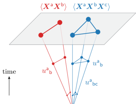
Figure 1: Schematic diagram of the cosmological flow. The time evolution of inflationary correlators, given by Eqs. (5a, 5b), is tracked from initial quantum fluctuations in the infinite past to the end of inflation. All the theory dependence is left in the precise form of the tensors $\tensor{u}{{}^{\sf{a}}}{{}_{\sf{b}}}$ and $\tensor{u}{{}^{\sf{a}}}{{}_{\sf{bc}}}$ driving this flow.

In this Letter and its companion paper Werth et al. (2023), we present the cosmological flow, a systematic framework to compute primordial corrrelators. It is based on solving differential equations in time to track the evolution of primordial correlators through the entire spacetime during inflation (see Fig. 1), for theories formulated straight at the level of fluctuations. In contrast to previous works Seery et al. (2012); Mulryne (2013); Dias et al. (2016); Mulryne and Ronayne (2018); Butchers and Seery (2018), our approach is not limited to particular background mechanisms. Instead, by adopting a philosophy that focuses on the study of correlators through effective field theories (EFT) of inflationary fluctuations, we are able to describe any theory. This allows us to obtain exact tree-level results in theories featuring an arbitrary number of fluctuating degrees of freedom with varied dispersion relations and masses, and coupled through any type of time-dependent interactions.

This work offers new possibilities for the study of inflationary correlators. One of the motivations for studying them lies in the appreciation that inflation is a one-of-a-kind window to probe fundamental physics at the highest reachable energies, comparable to the Hubble scale $H$ during inflation, which can be as high as $10^{14}$ GeV. Information about new physics—e.g. the presence of heavy particles of masses $m\sim H$—can be inferred from oscillatory patterns (or specific power law behaviors) present in the squeezed limit of the bispectrum Chen and Wang (2010); Noumi et al. (2013); Arkani-Hamed and Maldacena (2015). Our approach provides a systematic way to explore the characteristics of this cosmological collider signal in theories that are difficult to grasp analytically. First, as a heavy field weakly mixed with the curvature perturbation leads to the same cosmological collider frequency as a light but strongly mixed one, we show how complete predictions can be straightforwardly obtained in order to break theoretical degeneracies. We also present movies that display the cosmological flow of the bispectrum, therefore permitting to identify the characteristic times and scales at which the cosmological collider signal is building up. Second, we demonstrate that, due to the universal non-linearly realized boost symmetry, a time-dependent mixing—encompassing a wide range of inflationary models—leads to cosmological collider signals composed of modulated frequencies.

These results contradict some commonly held beliefs that the detection of such signals pinpoints the mass of a new particle. This highlights the importance of thoroughly studying signatures of all early-universe theories, as the cosmological flow approach enables one to do, for correctly interpreting cosmological data. More generally, our work paves the way for a far-reaching program of studying the phenomenology of inflationary correlators, shifting our focus from technical considerations to the unbiased exploration of the rich physics of inflation.

Primordial Fluctuations.

To begin, let us consider a set of bulk scalar degrees of freedom $\bm{\varphi}^{\alpha}(\bm{x},t)$, and $\bm{p}^{\beta}(\bm{x},t)$ the corresponding conjugate momenta. For practical purposes, we gather these fields and momenta in a phase-space vector $\bm{X}^{a}\equiv(\bm{\varphi}^{\alpha},\bm{p}^{\beta})$. We denote the corresponding operators in Fourier space with sans serif indices $\bm{X}^{\sf{a}}(\bm{k},t)$. They verify the canonical commutation algebra $[\bm{X}^{\sf{a}},\bm{X}^{\sf{b}}]=i\epsilon^{\sf{a}\sf{b}}$. These inflationary fluctuations are described by a Hamiltonian $H(\bm{\varphi}^{\alpha},\bm{p}^{\beta})$ which is a functional of the phase-space coordinates. Embracing an EFT point of view, it takes the form of a series expansion in powers of fluctuations

$$H=\frac{1}{2!}H_{\sf{ab}}\bm{X}^{\sf{a}}\bm{X}^{\sf{b}}+\frac{1}{3!}H_{\sf{abc}}\bm{X}^{\sf{a}}\bm{X}^{\sf{b}}\bm{X}^{\sf{c}}+\ldots\,,$$ (1)

where we adopt the extended Fourier summation convention for repeated indices to indicate a sum including integrals over Fourier modes. The tensors $H_{\sf{ab}},H_{\sf{abc}},\ldots$, which can be taken symmetric without loss of generality, are arbitrary functions of time and momenta. This form of the Hamiltonian is completely general and captures all theories involving scalar degrees of freedom at the level of inflationary fluctuations. The fully non-linear equations of motion read

$$\frac{\mathrm{d}\bm{X}^{\sf{a}}}{\mathrm{d}t} =i\,[H,\bm{X}^{\sf{a}}]$$ (2)

$$=\epsilon^{\sf{ac}}H_{\sf{cb}}\bm{X}^{\sf{b}}+\frac{1}{2!}\epsilon^{\sf{ad}}H_{\sf{dbc}}\bm{X}^{\sf{b}}\bm{X}^{\sf{c}}+\dots$$

$$=\tensor{u}{{}^{\sf{a}}}{{}_{\sf{b}}}\bm{X}^{\sf{b}}+\frac{1}{2!}\tensor{u}{{}^{\sf{a}}}{{}_{\sf{bc}}}\bm{X}^{\sf{b}}\bm{X}^{\sf{c}}+\ldots\,,$$

where the third line defines the tensors $\tensor{u}{{}^{\sf{a}}}{{}_{\sf{b}}},\tensor{u}{{}^{\sf{a}}}{{}_{\sf{bc}}},\dots$. Written in this form, it is clear that Eq. (2) encodes both the full classical evolution of $\bm{X}^{\sf{a}}$ and their quantum properties.

Time Evolution of Primordial Correlators.

We are interested in equal-time correlators of composite operators $\bra{\Omega}\mathcal{O}(\bm{X}^{\sf{a}})\ket{\Omega}$ evaluated at time $t$, where $\ket{\Omega}$ is the vacuum of the full interacting theory. Because the dynamics governed by Eq. (2) cannot be solved exactly in full generality, we choose the quadratic Hamiltonian $H_{0}=\frac{1}{2!}H_{\sf{ab}}\bm{X}^{\sf{a}}\bm{X}^{\sf{b}}$ to evolve the interaction-picture operators defined by $X^{\sf{a}}\equiv\mathcal{U}^{\dagger}\bm{X}^{\sf{a}}\,\mathcal{U}$, thus resorting to a perturbative description of the interactions encoded in $H_{\text{I}}=H-H_{0}$ Weinberg (2005b); Peskin and Schroeder (1995). This way, equal-time correlators are given by the well-known in-in formula Weinberg (2005a)

$$\bra{\Omega}\mathcal{O}(\bm{X}^{\sf{a}})\ket{\Omega}=\bra{0}\mathcal{U}\,\mathcal{O}(X^{\sf{a}})\,\mathcal{U}^{\dagger}\ket{0}\,,$$ (3)

where $\mathcal{U}=\bar{\text{T}}\exp(i\int_{-\infty(1-i\epsilon)}^{t}H_{\text{I}}(t^{\prime})\,\mathrm{d}t^{\prime})$ with $\bar{\text{T}}=\text{T}^{\dagger}$ the anti-time ordering operator, and $\ket{0}$ is the vacuum of the free theory. The $X^{\sf{a}}$ evolve with the full quadratic Hamiltonian. Working at tree-level and up to three-point correlators, one can expand the exponentials in Eq. (3) to obtain

$$\begin{aligned} \langle\bm{X}^{\sf{a}}\bm{X}^{\sf{b}}\rangle&=\bra{0}X^{\sf{a}}X^{\sf{b}}\ket{0}\,,\\ \langle\bm{X}^{\sf{a}}\bm{X}^{\sf{b}}\bm{X}^{\sf{c}}\rangle&=\bra{0}\frac{i}{3!}\int_{-\infty}^{t}\mathrm{d}t^{\prime}H_{\mathsf{def}}\left[X^{\mathsf{d}}X^{\mathsf{e}}X^{\mathsf{f}},X^{\mathsf{a}}X^{\mathsf{b}}X^{\mathsf{c}}\right]\ket{0}\,.\end{aligned}$$ (4)

For the three-point correlators, external operators are evaluated at the time $t$, and internal operators at time $t^{\prime}$. The simplicity of the cosmological flow lies in the ability to find, from first principles, a closed system of differential equations in time at the level of correlators Mulryne (2013). This cosmological flow is given by

$$\frac{\mathrm{d}}{\mathrm{d}t}\langle\bm{X}^{\sf{a}} \bm{X}^{\sf{b}}\rangle=\tensor{u}{{}^{\sf{a}}}{{}_{\sf{c}}}\langle\bm{X}^{\sf{c}}\bm{X}^{\sf{b}}\rangle+\tensor{u}{{}^{\sf{b}}}{{}_{\sf{c}}}\langle\bm{X}^{\sf{a}}\bm{X}^{\sf{c}}\rangle\,,$$ (5a)

$$\begin{split}\frac{\mathrm{d}}{\mathrm{d}t}\langle\bm{X}^{\sf{a}}\bm{X}^{\sf{b}}&\bm{X}^{\sf{c}}\rangle=\tensor{u}{{}^{\sf{a}}}{{}_{\sf{d}}}\langle\bm{X}^{\sf{d}}\bm{X}^{\sf{b}}\bm{X}^{\sf{c}}\rangle\\ &+\tensor{u}{{}^{\sf{a}}}{{}_{\sf{de}}}\langle\bm{X}^{\sf{b}}\bm{X}^{\sf{d}}\rangle\langle\bm{X}^{\sf{c}}\bm{X}^{\sf{e}}\rangle+(2\text{ perms})\,.\end{split}$$ (5b)

Eq. (5a) couples all two-point correlators, including those which contain conjugate momenta, and correctly capture all physical effects arising from quadratic operators in the theory. The structure of Eq. (5b) allows the flow of each kinematical configuration to be tracked separately. In Werth et al. (2023), we introduce handy diagrammatic rules to derive the differential equations governing the time evolution of any tree-level $n$-point correlator. Considering the Bunch-Davies state, as we do in the following, the initial conditions for Eqs. (5a, 5b) can be readily derived analytically provided one initializes the correlators sufficiently in the far past, see Werth et al. (2023) for explicit expressions. Naturally, the method equally works for any other state and is not restricted to inflation.

Goldstone Description.

We now apply this formalism to a concrete case. The spontaneous breaking of boost symmetry in cosmological backgrounds implies the unavoidable presence of a (canonically normalized) Goldstone boson $\pi_{c}(\bm{x},t)$ describing adiabatic fluctuations Creminelli et al. (2006); Cheung et al. (2008). At linear order, the field $\pi_{c}$ is related to the curvature perturbation by $\zeta=-Hc_{s}^{3/2}f_{\pi}^{-2}\pi_{c}$ where $c_{s}$ is the propagation speed of $\pi_{c}$ and $f_{\pi}^{4}\equiv 2M_{\rm pl}|\dot{H}|c_{s}$ is the symmetry breaking scale. Let us now consider an additional relativistic massive scalar field $\sigma(\bm{x},t)$ with mass $m$, coupled to $\pi_{c}$ through the following interacting Lagrangian, commonplace in concrete realizations of inflation:

$$\mathcal{L}/a^{3} =\rho\dot{\pi}_{c}\sigma+c_{s}^{3/2}\frac{\rho}{2f_{\pi}^{2}}\frac{(\partial_{i}\pi_{c})^{2}}{a^{2}}\sigma+c_{s}^{3/2}\frac{\dot{\rho}}{f_{\pi}^{2}}\,\pi_{c}\dot{\pi}_{c}\sigma$$ (6)

$$-\frac{1}{2\Lambda}\dot{\pi}_{c}^{2}\sigma-\frac{1}{2}\alpha\dot{\pi}_{c}\sigma^{2}-\mu\sigma^{3}\,,$$

where $\rho,\Lambda,\alpha$ and $\mu$ are—in general time-dependent—couplings. For the purpose of focusing on mixing interactions, we have omitted ever-present self-interactions of $\pi_{c}$ and have taken the decoupling limit where gravitational interactions vanish. Note that there is no a priori model-building requirement on the size of the dimensionless quadratic coupling $\rho/H$, and we allow this mixing parameter to be of order one or larger, which we call the strong mixing regime. A universal aspect is that this coupling $\rho$ fixes both the quadratic interaction $\dot{\pi}_{c}\sigma$ and the cubic interactions $(\partial_{i}\pi_{c})^{2}\sigma$ and $\pi_{c}\dot{\pi}_{c}\sigma$. This is a consequence of $\pi_{c}$ non-linearly realizing time diffeomorphisms, as these interactions are generated by the same operator $\rho(t)\delta g^{00}\sigma$ in the unitary gauge, after reintroducing the Goldstone boson $t\rightarrow t+\pi$ (see Werth et al. (2023) for more details). After performing a Legendre transform, the found Hamiltonian can be arranged in the form (1) in terms of the phase-space vector $\bm{X}^{a}=(\pi_{c},\sigma,p_{\pi},p_{\sigma})$. The identification of the tensors $\tensor{u}{{}^{\sf{a}}}{{}_{\sf{b}}}$ and $\tensor{u}{{}^{\sf{a}}}{{}_{\sf{bc}}}$ defined in Eq. (2) follows simply, see Werth et al. (2023).

Cosmological Colliders at Strong Mixing.

At tree-level, each cubic interaction in Eq. (6) gives an independent contribution to the bispectrum, and therefore can be treated separately. Following standard conventions Babich et al. (2004), we define the shape function $S$ such that

$$\braket{\zeta_{\bm{k}_{1}}\zeta_{\bm{k}_{2}}\zeta_{\bm{k}_{3}}}^{\prime}\equiv\frac{(2\pi)^{4}}{(k_{1}k_{2}k_{3})^{2}}\,\Delta_{\zeta}^{4}\,S(k_{1},k_{2},k_{3})\,,$$ (7)

where $\Delta_{\zeta}^{2}=\frac{k^{3}}{2\pi^{2}}\braket{\zeta_{\bm{k}}\zeta_{-\bm{k}}}^{\prime}$ is the dimensionless power spectrum of $\zeta$. The squeezed limit $k_{3}\ll k_{1}\simeq k_{2}$ is often described as a clean probe of the inflationary field content Chen and Wang (2010); Noumi et al. (2013); Arkani-Hamed and Maldacena (2015), notably with oscillations of the type $S\sim(k_{3}/k_{1})^{1/2}\cos(\mu\log(k_{3}/k_{1})+\varphi)$ revealing the spontaneous production, by the expansion of the universe, of a pair of scalar particles of masses $m/H=\sqrt{\mu^{2}+9/4}$. In Fig. (2), we compare these cosmological collider signals, obtained by numerically solving Eqs. (5a, 5b), for different constant quadratic mixing strengths, and for each cubic interaction in (6). The most distinctive feature is that the frequency of the oscillations is set by $\mu_{\text{eff}}^{2}=m_{\text{eff}}^{2}/H^{2}-9/4$, with $m^{2}_{\text{eff}}=m^{2}+\rho^{2}$ playing the role of the effective mass for $\sigma$ both at early and late times Castillo et al. (2014); An et al. (2018); Iyer et al. (2018); Werth et al. (2023). The appearance of the quadratic mixing in $m_{\text{eff}}$ can be interpreted as the result of resumming an infinite number of quadratic mixing insertions in the propagators of both fields, when using an interaction scheme where quadratic mixings are treated perturbatively. At strong mixing, the propagation of $\sigma$ is affected by the surrounding $\pi_{c}$ medium that interacts with it, leading to a self-energy correction. This is analogous to the electron self-energy correction in quantum electrodynamics due to its interaction with the photon Weinberg (2005b); Peskin and Schroeder (1995), the difference being that in our case such resummation occurs at tree-level because Lorentz invariance is spontaneously broken.

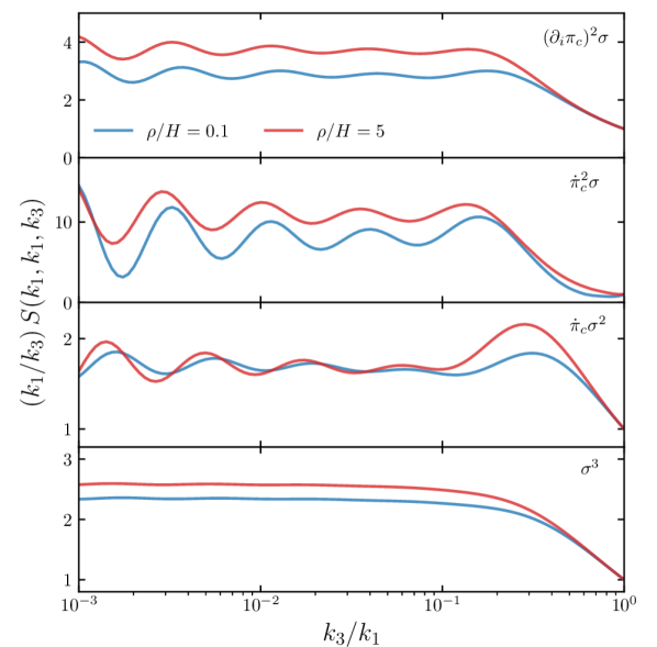
Figure 2: Squeezed limit of the shape functions for the four cubic interactions considered in Eq. (6) in the isosceles-triangle configuration $k_{1}=k_{2}$, for $c_{s}=0.1$ and $\mu_{\text{eff}}=5$ varying the quadratic mixing $\rho/H={\color[rgb]{0.12109375,0.46484375,0.70703125}0.1},{\color[rgb]{0.83984375,0.15234375,0.15625}5}$, corresponding to weak and strong mixings, respectively. For illustration purposes and to highlight the cosmological collider signal frequency, we have normalized the amplitudes of the signals to unity in the equilateral configuration $k_{1}=k_{2}=k_{3}$. We find that the amplitudes of the cosmological collider signals are non-monotonic as function of $\rho$, reaching a maximum for $\rho\sim m$ Werth et al. (2023).

Focusing on a single property of the signal like its frequency, as is usually advertised, one could wrongly interpret a future detection as the discovery of a new weakly mixed massive particle, whereas this may well correspond to the signature of a light particle, albeit strongly mixed to the curvature perturbation. Our approach precisely allows one to break such degeneracies by providing complete predictions—covering the frequency, amplitude and phase of the cosmological colliders, as well as contaminations from equilateral shapes—for any theory. This enables one to explore the full range of possible signals without working under the lamppost of analytical tractability. Moreover, the cosmological flow approach also enables one to reveal the dynamics of fluctuations, as we show in movies displaying how the cosmological collider signals are built differently as inflation proceeds, in theories with weak and strong mixing. This exemplifies how our method provides a powerful guide for physicists to test their theoretical understanding.

Cosmological Colliders with Features.

Focusing on inflationary fluctuations, the background dynamics is encoded in the time dependence of $H_{\sf{ab}},H_{\sf{abc}},\ldots$. Here we highlight the consequences of a time-dependent mixing on the cosmological collider signal. For definiteness, we consider $\rho(t)=\rho_{0}(a/a_{0})^{-n}\sin[\omega_{c}(t-t_{0})]$ with $n\geq 0$. The situation $n=0$ is relevant where the continuous shift symmetry of the Goldstone boson is broken to a discrete subgroup, see e.g. Behbahani et al. (2012), while $n=3/2$ is representative of, e.g. , background trajectories that undergo a sudden turn in field space, after which a massive field relaxes to its minimum subject to underdamped oscillations with frequency $\omega_{c}$. We neglect any time variation of the Hubble parameter $H$, of the mass of $\sigma$, and of the cubic interaction strengths in the second line of (6), as our purpose is to concentrate on what is imposed by symmetries. For simplicity, we also set $c_{s}=1$ and focus first on weak mixing $\rho_{0}<H$. The time-dependent mixing induces scale-dependent features in all correlation functions. For a fixed overall scale, the shape dependence of the cosmological collider depends on the cubic interaction that is considered. For those with constant strengths, the signal is conventional with frequency set by $\mu$ Chen et al. (2022). Instead, the cubic interactions dictated by the quadratic mixing are intrinsically time-dependent and have a special status, with $\dot{\rho}\,\pi_{c}\dot{\pi}_{c}\sigma$ dominant for rapid oscillations with $\mu_{c}\equiv\omega_{c}/H>1$.

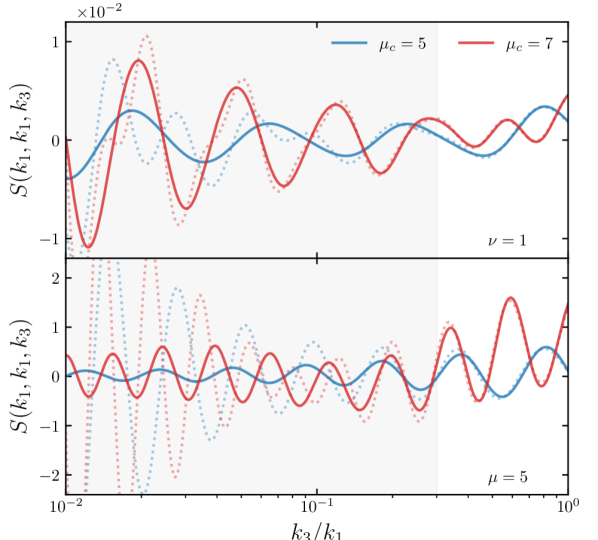
Figure 3: Shape dependence of the observable bispectrum (solid line) dictated by the time-dependent mixing $\rho(t)$, in the isosceles-triangle configuration $k_{1}=k_{2}$ at a fixed scale $\log(k_{3}/k_{0})=2$ where $k_{0}=(aH)(t_{0})$, for a light field $\nu=1$ (top) and a heavy field $\mu=5$ (bottom), varying the background frequency $\mu_{c}={\color[rgb]{0.12109375,0.46484375,0.70703125}5},{\color[rgb]{0.83984375,0.15234375,0.15625}7}$, and setting $n=0$. The observable signal is effectively reconstructed from the computed one (dotted line) upon meticulously subtracting the consistency relation $P_{\zeta}(k_{\textrm{S}})P_{\zeta}(k_{3})\mathrm{d}\log[k_{\textrm{S}}^{3}P_{\zeta}(k_{\textrm{S}})]/\mathrm{d}\log k_{\textrm{S}}$ with $\bm{k_{\textrm{S}}}=\bm{k}_{1}+\bm{k}_{3}/2$, inferred from the power spectrum $\braket{\zeta_{\bm{k}}\zeta_{-\bm{k}}}^{\prime}=P_{\zeta}(k)$. The shaded region corresponds to the squeezed limit where the templates (8) are valid. We have chosen $\rho_{0}/H=0.1$ to respect the current bounds on the power spectrum Akrami et al. (2020a).

We show in Fig. (3) the corresponding shape dependence of the bispectrum for a light and heavy field $\sigma$, for $n=0$ and different background frequencies $\mu_{c}$. These shapes are directly measurable in cosmological data as they already take into account the rescaling of the background by the long $\zeta$ mode Tanaka and Urakawa (2011); Pajer et al. (2013), yet leading to striking behaviours. In the squeezed limit, we find

$$S(k_{1},k_{1},k_{3})=\begin{cases}\left(\frac{k_{3}}{k_{1}}\right)^{1/2+n-\nu}\mathcal{A}\cos\left(\mu_{c}\log\left(\frac{k_{3}}{k_{1}}\right)+\varphi\right)\,,&\text{(light)}\\ \left(\frac{k_{3}}{k_{1}}\right)^{1/2+n}\left[\mathcal{A}_{+}\cos\left((\mu+\mu_{c})\log\left(\frac{k_{3}}{k_{1}}\right)+\varphi_{+}\right)+\mathcal{A}_{-}\cos\left((\mu-\mu_{c})\log\left(\frac{k_{3}}{k_{1}}\right)+\varphi_{-}\right)\right]\,,&\text{(heavy)}\end{cases}$$ (8)

where $\mu=\sqrt{(m/H)^{2}-9/4}$ and $\nu=i\mu$. Due to the dilution of the feature, the power-law scaling acquires an additional $(k_{3}/k_{1})^{n}$ suppression compared to the usual one Chen and Wang (2010). Depending on whether the field $\sigma$ is light ($m/H\leq 3/2$) or heavy ($m/H\geq 3/2$), the cosmological collider signal is either dictated by the background frequency $\mu_{c}$ or presents modulated frequencies in $\mu\pm\mu_{c}$, respectively. Remarkably, we find numerically that the templates (8) hold in the strong mixing regime. In Werth et al. (2023), we also provide analytical insights into these results, which provide a new way of probing the inflationary landscape. In particular, for light fields with $\nu>1/2+n$, we find that the oscillations modulate a growing envelope in the squeezed limit, which is expected to generate distinctive oscillations in the scale-dependent galaxy bias.

Conclusions.

The physics of inflation is phenomenologically rich and complex. In this Letter, we have presented a systematic framework for computing primordial correlators in any theory, focusing for definiteness on scalar degrees of freedom. Although massive fluctuations decay during inflation, their presence leaves a smoking-gun imprint in the squeezed limit of the observable bispectrum. Known as the cosmological collider signal, it offers a thrilling opportunity to identify new particles, in the same way as resonances for ground-based colliders. We demonstrated the power of our approach by computing cosmological collider signals in theories with strong and time-dependent mixings, and for various kinds of cubic interactions. These theoretically motivated scenarios present challenges that analytical methods are unable to address.

The cosmological flow provides the means for exploring and understanding inflationary physics in full generality, bridging the gap between theories and observations. To ensure its accessibility, we will make our new computational approach available as an open-source numerical tool. As natural extensions, we plan to incorporate spinning fields and higher-order correlation functions, as well as consider loops.

References

- Guth (1981) A. H. Guth, Phys. Rev. D 23, 347 (1981).
- Linde (1982) A. D. Linde, Phys. Lett. B 108, 389 (1982).
- Albrecht and Steinhardt (1982) A. Albrecht and P. J. Steinhardt, Phys. Rev. Lett. 48, 1220 (1982).
- Mukhanov and Chibisov (1981) V. F. Mukhanov and G. V. Chibisov, JETP Lett. 33, 532 (1981).
- Starobinsky (1982) A. A. Starobinsky, Phys. Lett. B 117, 175 (1982).
- Hawking (1982) S. W. Hawking, Phys. Lett. B 115, 295 (1982).
- Guth and Pi (1982) A. H. Guth and S. Y. Pi, Phys. Rev. Lett. 49, 1110 (1982).
- Bardeen et al. (1983) J. M. Bardeen, P. J. Steinhardt, and M. S. Turner, Phys. Rev. D 28, 679 (1983).
- Akrami et al. (2020a) Y. Akrami et al. (Planck), Astron. Astrophys. 641, A10 (2020a), arXiv:1807.06211 [astro-ph.CO] .
- Achúcarro et al. (2022) A. Achúcarro et al., (2022), arXiv:2203.08128 [astro-ph.CO] .
- Akrami et al. (2020b) Y. Akrami et al. (Planck), Astron. Astrophys. 641, A9 (2020b), arXiv:1905.05697 [astro-ph.CO] .
- Weinberg (2005a) S. Weinberg, Phys. Rev. D 72, 043514 (2005a), arXiv:hep-th/0506236 .
- Baumann and McAllister (2015) D. Baumann and L. McAllister, Inflation and String Theory, Cambridge Monographs on Mathematical Physics (Cambridge University Press, 2015) arXiv:1404.2601 [hep-th] .
- Werth et al. (2023) D. Werth, L. Pinol, and S. Renaux-Petel, (2023).
- Seery et al. (2012) D. Seery, D. J. Mulryne, J. Frazer, and R. H. Ribeiro, JCAP 09, 010 (2012), arXiv:1203.2635 [astro-ph.CO] .
- Mulryne (2013) D. J. Mulryne, JCAP 09, 010 (2013), arXiv:1302.3842 [astro-ph.CO] .
- Dias et al. (2016) M. Dias, J. Frazer, D. J. Mulryne, and D. Seery, JCAP 12, 033 (2016), arXiv:1609.00379 [astro-ph.CO] .
- Mulryne and Ronayne (2018) D. J. Mulryne and J. W. Ronayne, J. Open Source Softw. 3, 494 (2018), arXiv:1609.00381 [astro-ph.CO] .
- Butchers and Seery (2018) S. Butchers and D. Seery, JCAP 07, 031 (2018), arXiv:1803.10563 [astro-ph.CO] .
- Chen and Wang (2010) X. Chen and Y. Wang, JCAP 04, 027 (2010), arXiv:0911.3380 [hep-th] .
- Noumi et al. (2013) T. Noumi, M. Yamaguchi, and D. Yokoyama, JHEP 06, 051 (2013), arXiv:1211.1624 [hep-th] .
- Arkani-Hamed and Maldacena (2015) N. Arkani-Hamed and J. Maldacena, (2015), arXiv:1503.08043 [hep-th] .
- Weinberg (2005b) S. Weinberg, The Quantum theory of fields. Vol. 1 (Cambridge University Press, 2005).
- Peskin and Schroeder (1995) M. E. Peskin and D. V. Schroeder, An Introduction to quantum field theory (Addison-Wesley, Reading, USA, 1995).
- Creminelli et al. (2006) P. Creminelli, M. A. Luty, A. Nicolis, and L. Senatore, JHEP 12, 080 (2006), arXiv:hep-th/0606090 .
- Cheung et al. (2008) C. Cheung, P. Creminelli, A. L. Fitzpatrick, J. Kaplan, and L. Senatore, JHEP 03, 014 (2008), arXiv:0709.0293 [hep-th] .
- Babich et al. (2004) D. Babich, P. Creminelli, and M. Zaldarriaga, JCAP 08, 009 (2004), arXiv:astro-ph/0405356 .
- Castillo et al. (2014) E. Castillo, B. Koch, and G. Palma, JHEP 05, 111 (2014), arXiv:1312.3338 [hep-th] .
- An et al. (2018) H. An, M. McAneny, A. K. Ridgway, and M. B. Wise, JHEP 06, 105 (2018), arXiv:1706.09971 [hep-ph] .
- Iyer et al. (2018) A. V. Iyer, S. Pi, Y. Wang, Z. Wang, and S. Zhou, JCAP 01, 041 (2018), arXiv:1710.03054 [hep-th] .
- Behbahani et al. (2012) S. R. Behbahani, A. Dymarsky, M. Mirbabayi, and L. Senatore, JCAP 12, 036 (2012), arXiv:1111.3373 [hep-th] .
- Chen et al. (2022) X. Chen, R. Ebadi, and S. Kumar, JCAP 08, 083 (2022), arXiv:2205.01107 [hep-ph] .
- Tanaka and Urakawa (2011) T. Tanaka and Y. Urakawa, JCAP 05, 014 (2011), arXiv:1103.1251 [astro-ph.CO] .
- Pajer et al. (2013) E. Pajer, F. Schmidt, and M. Zaldarriaga, Phys. Rev. D 88, 083502 (2013), arXiv:1305.0824 [astro-ph.CO] .