Deep Dependency Networks for Multi-Label Classification

Abstract

We propose a simple approach which combines the strengths of probabilistic graphical models and deep learning architectures for solving the multi-label classification task, focusing specifically on image and video data. First, we show that the performance of previous approaches that combine Markov Random Fields with neural networks can be modestly improved by leveraging more powerful methods such as iterative join graph propagation, integer linear programming, and $\ell_{1}$ regularization-based structure learning. Then we propose a new modeling framework called deep dependency networks, which augments a dependency network, a model that is easy to train and learns more accurate dependencies but is limited to Gibbs sampling for inference, to the output layer of a neural network. We show that despite its simplicity, jointly learning this new architecture yields significant improvements in performance over the baseline neural network. In particular, our experimental evaluation on three video activity classification datasets: Charades, Textually Annotated Cooking Scenes (TACoS), and Wetlab, and three multi-label image classification datasets: MS-COCO, PASCAL VOC, and NUS-WIDE show that deep dependency networks are almost always superior to pure neural architectures that do not use dependency networks.

Keywords Multi-label Classification, Probabilistic Graphical Models, Multi-label Action Classification, Multi-label Image Classification, Dependency Networks

1 Introduction

In this paper, we focus on the multi-label classification (MLC) task, and more specifically on its two notable instantiations, multi-label action classification (MLAC) for videos and multi-label image classification (MLIC). At a high level, given a pre-defined set of labels (or actions) and a test example (video or image), the goal is to assign each test example to a subset of labels. It is well known that MLC is notoriously difficult because in practice the labels are often correlated, and thus predicting them independently may lead to significant errors. Therefore, most advanced methods explicitly model the relationship or dependencies between the labels, using either probabilistic techniques (Wang et al., 2008; Guo and Xue, 2013; Antonucci et al., 2013; Wang et al., 2014; Tan et al., 2015; Di Mauro et al., 2016) or non-probabilistic/neural methods (Kong et al., 2013; Papagiannopoulou et al., 2015; Chen et al., 2019a, b; Wang et al., 2021a; Nguyen et al., 2021; Wang et al., 2021b; Liu et al., 2021a; Qu et al., 2021).

To this end, motivated by approaches that combine probabilistic graphical models (PGMs) with neural networks (NNs) (Krishnan et al., 2015; Johnson et al., 2016), as a starting point, we investigated using (Conditional) Markov random fields (CRFs and MRFs), a type of undirected PGM, to capture the relationship between the labels as well as those between the labels and features derived from feature extractors. Unlike previous work, which used these MRF+NN or CRF+NN hybrids with conventional inference schemes such as Gibbs sampling (GS) and mean-field inference, our goal was to evaluate whether advanced approaches, specifically (1) iterative join graph propagation (IJGP) (Mateescu et al., 2010), a type of generalization Belief propagation technique (Yedidia et al., 2000), (2) integer linear programming (ILP) based techniques for computing most probable explanations and (3) a well-known structure learning method based on logistic regression with $\ell_{1}$-regularization (Lee et al., 2006; Wainwright et al., 2006), can improve the generalization performance of MRF+NN hybrids.

To measure and compare performance of these MRF+NN hybrids with NN models, we used several metrics such as mean average precision (mAP), label ranking average precision (LRAP), subset accuracy (SA), and the jaccard index (JI) and experimented on three video datasets: (1) Charades (Sigurdsson et al., 2016), (2) TACoS (Regneri et al., 2013) and (3) Wetlab (Naim et al., 2014) and three image datasets: (1) MS-COCO Lin et al. (2014), (2) PASCAL VOC 2007 Everingham et al. (2010) and (3) NUS-WIDE Chua et al. (2009). We found that generally speaking, both IJGP and ILP are superior to the baseline NN and Gibbs sampling in terms of JI and SA but are sometimes inferior to the NN in terms of mAP and LRAP. We speculated that because MRF structure learners only allow pairwise relationships and impose sparsity or low-treewidth constraints for faster, accurate inference, they often yield poor posterior probability estimates in high-dimensional settings. Since both mAP and LRAP require good posterior probability estimates, GS, IJGP, and ILP exhibit poor performance when mAP and LRAP are used to evaluate the performance.

To circumvent this issue and in particular to derive good posterior estimates, we propose a new PGM+NN hybrid called deep dependency networks (DDNs). At a high level, a dependency network (DN) (Heckerman et al., 2000) represents a joint probability distribution using a collection of conditional distributions, each defined over a variable (label) given all other variables (labels) in the network. Because each conditional distribution can be trained locally, DNs are easy to train. However, a caveat is that they are limited to Gibbs sampling for inference and are not amenable to advanced probabilistic inference techniques (Lowd, 2012).

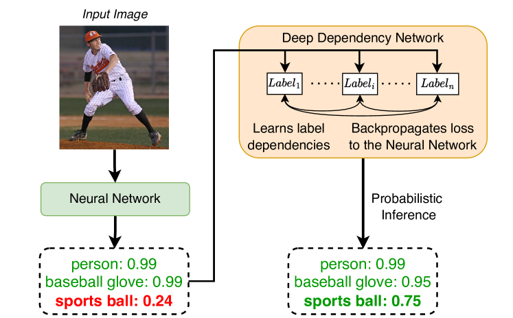
Figure 1: Illustration of improvements made by our proposed deep dependency network for multi-label image classification. The DDN learns label relationships, backpropagates the loss that reasons about label relationships to the neural network (NN) and helps to predict labels missed by the NN, such as the sports ball (occluded object).

In our proposed deep dependency network (DDN) architecture, a dependency network sits on top of a feature extractor based on a neural network. We illustrate the workings of the DDN architecture in Figure 1. The feature extractor converts the input image or video segment to a set of features, and the dependency network uses these features to define a local conditional distribution over each label given the features and other labels. We show that deep dependency models are easy to train either jointly or via a pipeline method where the feature extractor is trained first, followed by the DNN by defining an appropriate loss function that minimizes the negative pseudo log-likelihood (Besag, 1975) of the data. We conjecture that because DDNs can be quite dense, they often learn a better representation of the data, and as a result, they are likely to outperform MRFs learned from data in terms of posterior predictions.

We trained DDNs using the pipeline and joint learning approaches and evaluated them using the four aforementioned metrics (JI, SA, mAP and LRAP) and six datasets. We observed that jointly trained DDNs are often superior to the baseline neural networks as well as advanced MRF+NN methods that use GS, IJGP, and ILP on all four metrics. Specifically, they achieve the highest scores on all metrics on five out of the six datasets. Also, we found that the jointly trained DDNs are more accurate than the ones trained using the pipeline approach. This is because end-to-end (or joint) learning steers the feature selection process to provide tailored features for the DN, and learns a DN that is in-turn tailored to the output of this backbone. DDNs provide a multi-label classification head that works on the features extracted by the backbone.

In summary, this paper makes the following contributions:

• We propose a new hybrid model called deep dependency networks that combines the strengths of dependency networks (faster training and access to probabilistic inference schemes) and neural networks (flexibility, high-quality feature representation).

• We experimentally evaluate DDNs on three video datasets and three image datasets by using four metrics for solving the multi-label action classification and multi-label image classification tasks. This helps us to show that DDNs can be used for diverse multi-label classification tasks. We found that jointly trained DDNs consistently outperform NNs and MRF+NN hybrids on all metrics and datasets.

2 Preliminaries

A log-linear model or a Markov random field (MRF), denoted by $\mathcal{M}$, is an undirected probabilistic graphical model (Koller and Friedman, 2009) that is widely used in many real-world domains for representing and reasoning about uncertainty. It is defined as a triple $\langle{\mathbf{X}},\mathcal{F},\Theta\rangle$ where ${\mathbf{X}}{}=\{X_{1},\ldots,X_{n}\}$ is a set of Boolean random variables, $\mathcal{F}=\{f_{1},\ldots,f_{m}\}$ is a set of features such that each feature $f_{i}$ (we assume that a feature is a Boolean formula) is defined over a subset ${\mathbf{D}}_{i}$ of ${\mathbf{X}}$, and $\Theta=\{\theta_{1},\ldots,\theta_{m}\}$ is a set of real-valued weights or parameters, namely $\forall\theta_{i}\in\Theta;\;\theta_{i}\in\mathbb{R}$ such that each feature $f_{i}$ is associated with a parameter $\theta_{i}$. $\mathcal{M}$ represents the following probability distribution:

$$P({\mathbf{x}})=\frac{1}{Z(\Theta)}\exp\left\{\sum_{i=1}^{m}\theta_{i}f_{i}\left({\mathbf{x}}_{{\mathbf{D}}_{i}}\right)\right\}$$ (1)

where ${\mathbf{x}}$ is an assignment of values to all variables in ${\mathbf{X}}$, ${\mathbf{x}}_{{\mathbf{D}}_{i}}$ is the projection of ${\mathbf{x}}$ on the variables ${\mathbf{D}}_{i}$ of $f_{i}$, $f_{i}({\mathbf{x}}_{{\mathbf{D}}_{i}})$ is an indicator function that equals $1$ when the assignment ${\mathbf{x}}_{{\mathbf{D}}_{i}}$ evaluates $f_{i}$ to True and is $0$ otherwise, and $Z(\Theta)$ is the normalization constant called the partition function.

We focus on three tasks over MRFs: (1) structure learning which is the problem of learning the features and parameters given training data; (2) posterior marginal inference which is the task of computing the marginal probability distribution over each variable in the network given evidence (evidence is defined as an assignment of values to a subset of variables); and (3) finding the most likely assignment to all the non-evidence variables given evidence (this task is often called maximum-a-posteriori or MAP inference in short). All of these tasks are at least NP-hard in general and therefore approximate methods are often preferred over exact ones in practice.

A popular and fast method for structure learning is to learn binary pairwise MRFs by training an $\ell_{1}$-regularized logistic regression classifier for each variable given all other variables as features (Wainwright et al., 2006; Lee et al., 2006). $\ell_{1}$-regularization induces sparsity in that it encourages many weights to take the value zero. All non-zero weights are then converted into conjunctive features. Each conjunctive feature evaluates to True if both variables are assigned the value $1$ and to False otherwise. Popular approaches for posterior marginal inference are the Gibbs sampling algorithm and generalized Belief propagation (Yedidia et al., 2000) techniques such as Iterative Join Graph Propagation (Mateescu et al., 2010). For MAP inference, a popular approach is to encode the optimization problem as a linear integer programming problem (Koller and Friedman, 2009) and then use off-the-shelf approaches such as (Gurobi Optimization, LLC, 2022) to solve the latter.

Dependency Networks (DNs) (Heckerman et al., 2000) represent the joint distribution using a set of local conditional probability distributions, one for each variable. Each conditional distribution defines the probability of a variable given all of the others. A DN is consistent if there exists a joint probability distribution $P({\mathbf{x}})$ such that all conditional distributions $P_{i}(x_{i}|{\mathbf{x}}_{-i})$ where ${\mathbf{x}}_{-i}$ is the projection of ${\mathbf{x}}$ on ${\mathbf{X}}\setminus\{X_{i}\}$, are conditional distributions of $P({\mathbf{x}})$.

A DN is learned from data by learning a classifier (e.g., logistic regression, multi-layer perceptron, etc.) for each variable, and thus DN learning is embarrassingly parallel. However, because the classifiers are independently learned from data, we often get an inconsistent DN. It has been conjectured (Heckerman et al., 2000) that most DNs learned from data are almost consistent in that only a few parameters need to be changed in order to make them consistent.

The most popular inference method over DNs is fixed-order Gibbs sampling (Liu, 2008). If the DN is consistent, then its conditional distributions are derived from a joint distribution $P({\mathbf{x}})$, and the stationary distribution (namely the distribution that Gibbs sampling converges to) will be the same as $P({\mathbf{x}})$. If the DN is inconsistent, then the stationary distribution of Gibbs sampling will be inconsistent with the conditional distributions.

3 Deep Dependency Networks

In this section, we describe how to solve the multi-label action classification task in videos and the multi-label image classification task using a hybrid of dependency networks and neural networks. At a high level, the neural network provides high-quality features given video segments/images and the dependency network represents and reasons about the relationships between the labels and features.

3.1 Framework

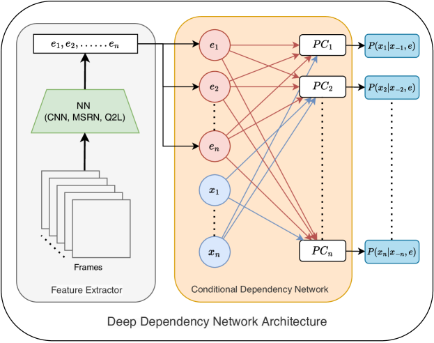
Figure 2: Illustration of Dependency Network for multi-label video classification. The NN takes video clips (frames) as input and outputs the features $E_{1},E_{2},...,E_{n}$ (denoted by red colored nodes) for the DN. These features are then used by the probabilistic classifiers ($PC_{1}$, $\ldots$, $PC_{n}$) to model the local conditional distributions. At each output node (blue boxes), the form of the conditional distribution is variable given its parents (incoming arrows represented by orange and blue color) in the conditional dependency network.

Let ${\mathbf{V}}$ denote the set of random variables corresponding to the pixels and ${\mathbf{v}}$ denote the RGB values of the pixels in a frame or a video segment. Let ${\mathbf{E}}$ denote the (continuous) output nodes of a neural network which represents a function $\mathbb{N}:{\mathbf{v}}\rightarrow{\mathbf{e}}$, that takes ${\mathbf{v}}$ as input and outputs an assignment ${\mathbf{e}}$ to ${\mathbf{E}}$. Let ${\mathbf{X}}=\{X_{1},\ldots,X_{n}\}$ denote the set of labels (actions). For simplicity, we assume that $|{\mathbf{E}}|=|{\mathbf{X}}|=n$. Given $({\mathbf{V}},{\mathbf{E}},{\mathbf{X}})$, a deep dependency network (DDN) is a pair $\langle\mathcal{N},\mathcal{D}\rangle$ where $\mathcal{N}$ is a neural network that maps ${\mathbf{V}}={\mathbf{v}}$ to ${\mathbf{E}}={\mathbf{e}}$ and $\mathcal{D}$ is a conditional dependency network (Guo and Gu, 2011) that models $P({\mathbf{x}}|{\mathbf{e}})$ where ${\mathbf{e}}=\mathbb{N}({\mathbf{v}})$. The conditional dependency network represents the distribution $P({\mathbf{x}}|{\mathbf{e}})$ using a collection of local conditional distributions $P_{i}(x_{i}|{\mathbf{x}}_{-i},{\mathbf{e}})$, one for each label $X_{i}$, where ${\mathbf{x}}_{-i}=\{x_{1},\ldots,x_{i-1},x_{i+1},\ldots,x_{n}\}$.

Thus, a DDN is a discriminative model and represents the conditional distribution $P({\mathbf{x}}|{\mathbf{v}})$ using several local conditional distributions $P(x_{i}|{\mathbf{x}}_{-i},{\mathbf{e}})$ and makes the following conditional independence assumptions $P(x_{i}|{\mathbf{x}}_{-i},{\mathbf{v}})=P(x_{i}|{\mathbf{x}}_{-i},{\mathbf{e}})$ where ${\mathbf{e}}=\mathbb{N}({\mathbf{v}})$. Figure  2 shows the architecture of a DDN for solving the multi-label action classification task in videos.

3.2 Learning

We can either train the DDN using a pipeline method or via joint training. In the pipeline method, we first train the neural network using standard approaches (e.g., using cross-entropy loss) or use a pre-trained model. Then for each training example $({\mathbf{v}},{\mathbf{x}})$, we send the video/image through the neural network to obtain a new representation ${\mathbf{e}}$ of ${\mathbf{v}}$. The aforementioned process transforms each training example $({\mathbf{v}},{\mathbf{x}})$ into a new feature representation $({\mathbf{e}},{\mathbf{x}})$ where ${\mathbf{e}}=\mathbb{N}({\mathbf{v}})$. Finally, for each label $X_{i}$, we learn a classifier to model the conditional distribution $P_{i}(x_{i}|{\mathbf{x}}_{-i},{\mathbf{e}})$. Specifically, given a training example $({\mathbf{e}},{\mathbf{x}})$, each probabilistic classifier indexed by $i$ ($PC_{i}$), uses $X_{i}$ as the class variable and $({\mathbf{E}}\cup{\mathbf{X}}_{-i})$ as the attributes. In our experiments, we used two probabilistic classifiers, logistic regression and multi-layer perceptron.

The pipeline method has several useful properties: it requires modest computational resources, is relatively fast and can be easily parallelized. As a result, it is especially beneficial when (only) less powerful GPUs are available at training time but a pre-trained network that is trained using more powerful GPUs is readily available.

For joint learning, we propose to use the conditional pseudo log-likelihood loss (CPLL) Besag (1975). Let $\Theta$ denote the set of parameters of the DDN, then the CPLL is given by

$$\mathcal{L}(\Theta,{\mathbf{v}},{\mathbf{x}}) =-\sum_{i=1}^{n}\log P_{i}(x_{i}|{\mathbf{v}},{\mathbf{x}}_{-i};\Theta)$$ (2)

$$=-\sum_{i=1}^{n}\log P_{i}(x_{i}|{\mathbf{e}}=\mathbb{N}({\mathbf{v}}),{\mathbf{x}}_{-i};\Theta)$$ (3)

In practice, for faster training/convergence, we will partition the parameters $\Theta$ of the DDN into two (disjoint) subsets $\Pi$ and $\Gamma$ where $\Pi$ and $\Gamma$ denote the parameters of the neural network and local conditional distributions respectively; and initialize $\Pi$ using a pre-trained neural network and $\Gamma$ using the pipeline method. Then, we can use any gradient-based (backpropagation) method to minimize the loss function.

3.3 Inference: Using the DDN to Make Predictions

Unlike a conventional discriminative model such as a neural network, in a DDN, we cannot predict the output labels by simply making a forward pass over the network. This is because each probabilistic classifier indexed by $i$ (which yields a probability distribution over $X_{i}$) requires an assignment ${\mathbf{x}}_{-i}$ to all labels except $x_{i}$, and ${\mathbf{x}}_{-i}$ is not available at prediction time.

To address this issue, we use the following Gibbs sampling based approach (a detailed algorithm is provided in the appendix). We first send the frame/segment ${\mathbf{v}}$ through the neural network $\mathcal{N}$ to yield an assignment ${\mathbf{e}}$ to the output nodes of the neural network. Then, we perform fixed-order Gibbs Sampling over the dependency network where the latter represents the distribution $P({\mathbf{x}}|{\mathbf{e}})$. Finally, given samples $({\mathbf{x}}^{(1)},\ldots,{\mathbf{x}}^{(N)})$ generated via Gibbs sampling, we estimate the marginal probability distribution of each label $X_{i}$ using the following mixture estimator (Liu, 2008):

$$\hat{P}_{i}\left(x_{i}|{\mathbf{v}}\right)=\frac{1}{N}\sum_{j=1}^{N}P_{i}\left(x_{i}\mid{\mathbf{x}}_{-i}^{(j)},{\mathbf{e}}\right)$$ (4)

4 Experimental Evaluation

In this section, we evaluate the proposed models on two multi-label classification tasks: (1) multi-label activity classification using three video datasets; and (2) multi-label image classification using three image datasets. We begin by describing the datasets and metrics, followed by the experimental setup, and conclude with the results. All models were implemented using PyTorch, and one NVIDIA A40 GPU was used to train and test all the models.

4.1 Datasets and Metrics

We evaluated our algorithms on the following three video datasets: (1) Charades (Sigurdsson et al., 2016); (2) Textually Annotated Cooking Scenes (TACoS) (Regneri et al., 2013); and (3) Wetlab (Naim et al., 2015). In the Charades dataset, the videos are divided into segments (video clips), and each segment is annotated with one or more action labels. In the TACoS and Wetlab datasets, each frame is associated with one or more actions.

Charades dataset (Sigurdsson et al., 2016) comprises of videos of people performing daily indoor activities while interacting with various objects. In the standard split, there are 7,986 training videos and 1,863 validation videos. We used the training videos to train the models and the validation videos for testing purposes. We follow the instructions provided in PySlowFast (Fan et al., 2020) to do the train-test split for the dataset. The dataset has roughly 66,500 temporal annotations for 157 action classes.

The TaCOS dataset (Regneri et al., 2013) consists of third-person videos of a person cooking in a kitchen. The dataset comes with hand-annotated labels of actions, objects, and locations for each video frame. From the complete set of these labels, we selected 28 labels. By dividing the videos corresponding to these labels into train and test sets, we get a total of 60,313 frames for training and 9,355 frames for testing, spread out over 17 videos.

The Wetlab dataset (Naim et al., 2014) comprises of videos where experiments are being performed by lab technicians that involve hazardous chemicals in a wet laboratory. We used five videos for training and one video for testing. The training set comprises 100,054 frames, and the test set comprises 11,743 frames. There are 57 possible labels and each label corresponds to an object or a verb, and each action is made of one or more labels from each category.

We also evaluated our algorithms on three multi-label image classification (MLIC) datasets: (1) MS-COCO (Lin et al., 2014); (2) PASCAL VOC 2007, and (Everingham et al., 2010); and (3) NUS-WIDE (Chua et al., 2009).

MS-COCO (Microsoft Common Objects in Context) (Lin et al., 2014) is a large-scale object detection and segmentation dataset. It has also been extensively used for the MLIC task. The dataset contains 122,218 labeled images and 80 labels in total. Each image is labeled with at least 2.9 labels on average. We used the 2014 version of the dataset.

NUS-WIDE dataset (Chua et al., 2009) is a real-world web image dataset that contains 269,648 images from Flickr. Each image has been manually annotated with a subset of 81 visual classes that include objects and scenes.

PASCAL VOC 2007 (Everingham et al., 2010) is another dataset that has been used widely for the MLIC task. The dataset contains 5,011 images in the train-validation set and 4,952 images in the test set. The total number of labels in the dataset is 20 which corresponds to object classes.

We follow the instructions provided in (Qu et al., 2021) to do the train-test split for NUS-WIDE and PASCAL VOC 2007. We evaluated the performance on the TACoS, Wetlab, MS-COCO, NUS-WIDE, and VOC datasets using the following four metrics: mean Average Precision (mAP), Label Ranking Average Precision (LRAP), Subset Accuracy (SA), and Jaccard Index (JI). For all the metrics that are being considered here, a higher value means better performance. mAP and LRAP require access to an estimate of the posterior probability distribution at each label while SA and JI are non-probabilistic and only require an assignment to the labels. Note that we only report mAP, LRAP and JI on the Charades dataset because existing approaches cannot achieve reasonable SA due to large size of the label space.

In recent years, mAP has been used as an evaluation metric for multi-label image and action classification in lieu of conventional metrics such as SA and JI. However, both SA (which seeks exact match with the ground truth) and JI are critical for applications such as dialogue systems (Vilar et al., 2004), self-driving cars (Chen et al., 2019c; Protopapadakis et al., 2020) and disease diagnosis (Maxwell et al., 2017; Zhang et al., 2019; Zhou et al., 2021) where MLC is one of the sub-tasks in a series of interrelated sub-tasks. Missing a single label in these applications could have disastrous consequences for downstream sub-tasks.

4.2 Experimental Setup and Methods

We used three types of architectures in our experiments: (1) Baseline neural networks which are specific to each dataset; (2) neural networks augmented with MRFs, which we will refer to as deep random fields or DRFs in short; and (3) the method proposed in this paper which uses a dependency network on top of the neural networks called deep dependency networks (DDNs).

Neural Networks. We choose four different types of neural networks, and they act as a baseline for the experiments and as a feature extractor for DRFs and DDNs. Specifically, we experimented with: (1) 2D CNN, (2) 3D CNN, (3) transformers, and (4) CNN with attention module and graph attention networks (GAT) (Veličković et al., 2018). This helps us show that our proposed method can improve the performance of a wide variety of neural architectures, even those which model label relationships because unlike the latter it performs probabilistic inference (Gibbs sampling).

For the Charades dataset, we use the PySlowFast (Fan et al., 2020) implementation of the SlowFast Network (Feichtenhofer et al., 2019) (a state-of-the-art 3D CNN for video classification) which uses a 3D ResNet model as the backbone. For TACoS and Wetlab datasets, we use InceptionV3 (Szegedy et al., 2016), one of the state-of-the-art 2D CNN models for image classification. For the MS-COCO dataset, we used Query2Label (Q2L) Liu et al. (2021a), which uses transformers to pool class-related features. Q2L also learns label embeddings from data to capture the relationships between the labels. Finally, we used the multi-layered semantic representation network (MSRN) (Qu et al., 2021) for NUS-WIDE and PASCAL VOC. MSRN also models label correlations and learns semantic representations at multiple convolutional layers. For extracting the features for Charades, MS-COCO, NUS-WIDE, and PASCAL VOC datasets, we use the pre-trained models and hyper-parameters provided in their respective repositories. For TaCOS and Wetlab datasets, we fine-tuned an InceptionV3 model that was pre-trained on the ImageNet dataset.

Deep Random Fields (DRFs). As a baseline, we used a model that combines MRFs with neural networks. This DRF model is similar to the DDN except that we use an MRF instead of a DDN to compute $P({\mathbf{x}}|{\mathbf{e}})$. We trained the MRFs generatively; namely, we learned a joint distribution $P({\mathbf{x}},{\mathbf{e}})$, which can be used to compute $P({\mathbf{x}}|{\mathbf{e}})$ by instantiating evidence. We chose generative learning because we learned the structure of the MRFs from data, and discriminative structure learning is slow in practice (Koller and Friedman, 2009). Specifically, we used the logistic regression with $\ell_{1}$ regularization method of (Wainwright et al., 2006) to learn a pairwise MRF. The training data for this method is obtained by sending each annotated video clip (or frame) $({\mathbf{v}},{\mathbf{x}})$ through the neural network and transforming it to $({\mathbf{e}},{\mathbf{x}})$ where ${\mathbf{e}}=\mathbb{N}({\mathbf{v}})$. At termination, this method yields a graph ${\mathcal{G}}$ defined over ${\mathbf{X}}\cup{\mathbf{E}}$.

For parameter/weight learning, we converted each edge over ${\mathbf{X}}\cup{\mathbf{E}}$ to a conjunctive feature. For example, if the method learns an edge between $X_{i}$ and $E_{j}$, we use a conjunctive feature $X_{i}\wedge E_{j}$ which is true if both $X_{i}$ and $E_{j}$ are assigned the value $1$. Then we learned the weights for each feature by maximizing the pseudo log-likelihood of the data.

For inference over MRFs, we used Gibbs sampling (GS), Iterative Join Graph Propagation (IJGP) Mateescu et al. (2010), and Integer Linear Programming (ILP) methods. Thus, three versions of DRFs corresponding to the inference scheme were used. We refer to these schemes as DRF-GS, DRF-ILP, and DRF-IJGP, respectively. Note that IJGP and ILP are advanced schemes, and we are unaware of their use for multi-label classification. Our goal is to test whether advanced inference schemes help improve the performance of deep random fields.

Deep Dependency Networks (DDNs). We experimented with four versions of DDNs: (1) DDN-LR-Pipeline; (2) DDN-MLP-Pipeline; (3) DDN-LR-Joint; and (4) DDN-MLP-Joint. The first and third versions use logistic regression (LR), while the second and fourth versions use multi-layer perceptrons (MLP) to represent the conditional distributions. The first two versions are trained using the pipeline method, while the last two versions are trained using the joint learning loss given in equation 3.

Hyperparameters. For DRFs, in order to learn a sparse structure (using the logistic regression with $\ell_{1}$ regularization method of (Wainwright et al., 2006)), we increased the regularization constant associated with the $\ell_{1}$ regularization term until the number of neighbors of each node in ${\mathcal{G}}$ is bounded between 2 and 10. We enforced this sparsity constraint in order to ensure that the inference schemes (specifically, IJGP and ILP) are accurate and the model does not overfit to the training data. IJGP, ILP, and GS are anytime methods; for each, we used a time-bound of 60 seconds per example.

For DDNs, we used LR with $\ell_{1}$ regularization and MLPs with $\ell_{2}$ regularization. For MLP the number of hidden layers was selected from the $\{2,3,4\}$. The regularization constants for LR and MLP (chosen from the $\{0.1,0.01,0.001\}$) and the number of layers for MLP were chosen via cross-validation. For all datasets, MLP with four layers performed the best. ReLU was used for the activation function for each hidden layer and sigmoid for the outputs. For joint learning, we reduced the learning rates of both LR and MLP models by expanding on the learning rate scheduler given in PySlowFast (Fan et al., 2020) and the initial learning rate was chosen in the range of $\displaystyle[10^{-3},10^{-5}]$.

4.3 Results

Table 1: Comparison of our methods with the baseline for MLAC task. The best/second best values are bold/underlined. The last row shows the relative improvement made by the best performing proposed method over the baseline.

Method	Charades			TACoS				Wetlab
	mAP ↑	LRAP ↑	JI ↑	mAP ↑	LRAP ↑	SA ↑	JI ↑	mAP ↑	LRAP ↑	SA ↑	JI ↑
SlowFast(Fan et al., 2020)	0.388	0.535	0.294
InceptionV3(Szegedy et al., 2016)				0.701	0.808	0.402	0.608	0.791	0.821	0.353	0.638
DRF - GS	0.265	0.439	0.224	0.558	0.794	0.469	0.650	0.539	0.757	0.353	0.515
DRF - ILP	0.193	0.278	0.306	0.403	0.672	0.509	0.647	0.630	0.734	0.597	0.727
DRF - IJGP	0.312	0.437	0.319	0.561	0.814	0.439	0.701	0.788	0.853	0.580	0.737
DDN - LR - Pipeline	0.345	0.484	0.290	0.716	0.826	0.504	0.672	0.775	0.855	0.573	0.702
DDN - LR - Joint	0.396	0.548	0.313	0.746	0.839	0.537	0.686	0.843	0.869	0.634	0.779
DDN - MLP - Pipeline	0.375	0.549	0.295	0.729	0.860	0.579	0.695	0.812	0.882	0.618	0.727
DDN - MLP - Joint	0.407	0.554	0.341	0.780	0.875	0.596	0.704	0.881	0.897	0.697	0.792
Relative Improvement (%)	4.85	3.66	15.93	11.20	8.37	48.43	15.82	11.34	9.26	97.66	24.15

Table 2: Comparison of our methods with the baseline for MLIC task. The best/second best values are bold/underlined. The last row shows the relative improvement made by the best-performing proposed method over the baseline.

Method	MS-COCO				NUS-WIDE				PASCAL-VOC
	mAP ↑	LRAP ↑	SA ↑	JI ↑	mAP ↑	LRAP ↑	SA ↑	JI ↑	mAP ↑	LRAP ↑	SA ↑	JI ↑
Q2L Liu et al. (2021a)	0.912	0.961	0.507	0.802
MSRN (Qu et al., 2021)					0.615	0.845	0.314	0.638	0.960	0.976	0.708	0.853
DRF - GS	0.751	0.861	0.347	0.692	0.401	0.739	0.282	0.547	0.767	0.933	0.727	0.834
DRF - ILP	0.735	0.825	0.545	0.817	0.252	0.591	0.322	0.590	0.809	0.879	0.761	0.876
DRF - IJGP	0.741	0.902	0.546	0.818	0.410	0.752	0.344	0.628	0.832	0.941	0.763	0.869
DDN - LR - Pipeline	0.830	0.924	0.496	0.785	0.432	0.797	0.306	0.586	0.884	0.932	0.684	0.787
DDN - LR - Joint	0.841	0.928	0.546	0.816	0.501	0.821	0.325	0.623	0.924	0.962	0.761	0.869
DDN - MLP - Pipeline	0.876	0.945	0.556	0.821	0.561	0.830	0.332	0.632	0.927	0.956	0.766	0.876
DDN - MLP - Joint	0.903	0.958	0.586	0.837	0.615	0.847	0.356	0.660	0.964	0.983	0.805	0.912
Relative Improvement (%)	-1.05	-0.23	15.44	4.27	0.00	0.29	13.42	3.50	0.37	0.74	13.70	6.84

We compare the baseline neural networks with three versions of DRFs and four versions of DDNs using the four metrics and six datasets given in Section 4.1. The results are presented in tables 1 and 2. We also show the improvements that our method makes over the baseline. Further evaluation on PASCAL-VOC and MS-COCO datasets can be found in the appendix, where we provide comparison between the proposed method and other state-of-the-art methods.

Comparison between Baseline neural network and DRFs. We observe that IJGP and ILP outperform the baseline neural networks (which includes transformers for some datasets) in terms of the two non-probabilistic metrics JI and SA on five out of the six datasets. IJGP typically outperforms GS and ILP on JI. ILP outperforms the baseline on SA (notice that SA is 1 if there is an exact match between predicted and true labels and 0 otherwise) because it performs an accurate maximum-a-posteriori (MAP) inference (accurate MAP inference on an accurate model is likely to yield high SA). However, on metrics that require estimating the posterior probabilities, mAP and LRAP, the DRF schemes sometimes hurt the performance and at other times are only marginally better than the baseline methods. We observe that advanced inference schemes, particularly IJGP and ILP are superior on average to GS. Note that getting a higher SA is much harder in datasets having high label cardinalities. Specifically, SA does not distinguish between models that predict almost correct labels and completely incorrect outputs.

Comparison between Baseline neural networks and DDNs. We observe that the best performing DDN model, DDN-MLP with joint learning, outperforms the baseline neural networks on five out of the six datasets on all metrics. Sometimes, the improvement is substantial (e.g., 9% improvement in mAP on the wetlab dataset). The DDN-MLP model with joint learning improves considerably over the baseline method when performance is measured using SA and JI while keeping the precision comparative or higher. Roughly speaking, the MLP versions are superior to the LR versions, and the joint models are superior to the ones trained using the pipeline method. On the non-probabilistic metrics (JI and SA), the pipeline models are often superior to the baseline neural network, while on the mAP metric, they may hurt the performance.

We observe that on the MLIC task, the DDN methods outperform Q2L and MSRN, even though both Q2L and MSRN model label correlations. This suggests that DDNs are either able to uncover additional relationships between labels during the learning phase or better reason about them during the inference (Gibbs sampling) phase or both. In particular, both Q2L and MSRN do not use Gibbs sampling to predict the labels, because they do not explicitly model the joint probability distribution over the labels.

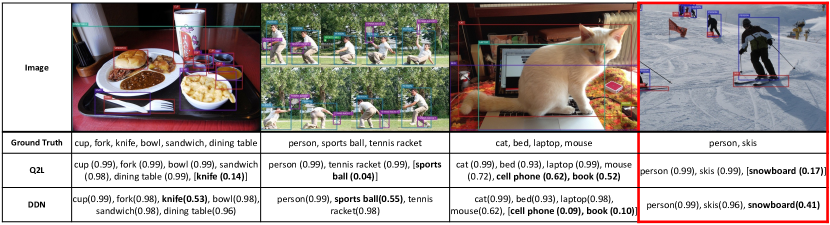
Figure 3: Comparison of labels predicted by Q2L Liu et al. (2021a) and our DDN-MLP-Joint model on the MS-COCO dataset. Labels in bold represent the difference between the predictions of the two methods assuming that a threshold of 0.3 is used (i.e., every label whose probability $>0.3$ is considered as a predicted label). We also provide the probabilities in (). Labels enclosed in [] denote the labels that were not predicted by the corresponding method (added to compare the probabilities). The first three column shows examples where DDN improves over Q2L, while the last column (outlined in red) shows an example where DDN is worse than Q2L.

In Figure 3, we show a few images and their corresponding labels predicted using Q2L and DDN-MLP-Joint on the MS-COCO dataset. These results show that our method not only adds labels missed by Q2L but also removes several incorrect predictions. For example, in the first and second images, our method adds labels missed by Q2L and aligns the results perfectly with the ground truth. In the third image, our proposed method removes incorrect predictions. In the last image, we show an example where the DDN performs worse than Q2L and adds a label that is not in the ground truth. More examples are provided in the appendix.

Comparison between DRFs and DDNs. We observe that the jointly trained DDNs are almost always superior to the best-performing DRFs on all datasets. Interestingly, on average, the pipeline DDN models outperform the DRF models when performance is measured using the mAP and LRAP metrics. However, when the SA and JI metrics are used, we observe that there is no significant difference in performance between pipeline DDNs and DRFs. Thus, DRFs can be especially beneficial if there are no GPU resource available for training and we want to optimize for JI or SA.

In summary, jointly trained deep dependency networks are superior to the baseline neural networks as well as the models that combine Markov random fields and neural networks. The experimental results on MLC clearly demonstrate the practical usefulness of our proposed method.

5 Related Work

A large number of methods have been proposed that train PGMs and NNs jointly. For example, (Zheng et al., 2015) proposed to combine conditional random fields (CRFs) and recurrent neural networks (RNNs), (Schwing and Urtasun, 2015; Larsson et al., 2017, 2018; Arnab et al., 2016) showed how to combine CNNs and CRFs, (Chen et al., 2015) proposed to use densely connected graphical models with CNNs, and (Johnson et al., 2016) combined latent graphical models with neural networks. As far as we know, ours is the first work that shows how to jointly train a dependency network, neural network hybrid. Another virtue of DDNs is that they are easy to train and parallelizable, making them an attractive choice.

The combination of PGMs and NNs has been applied to improve performance on a wide variety of real-world tasks. Notable examples include human pose estimation (Tompson et al., 2014; Liang et al., 2018; Song et al., 2017; Yang et al., 2016a), semantic labeling of body parts (Kirillov et al., 2016), stereo estimation Knöbelreiter et al. (2017), language understanding (Yao et al., 2014), joint intent detection and slot filling (Xu and Sarikaya, 2013), polyphonic piano music transcription (Sigtia et al., 2016), face sketch synthesis Zhu et al. (2021), sea ice floe segmentation (Nagi et al., 2021) and crowd-sourcing aggregation (Li et al., 2021)). These hybrid models have also been used for solving a range of computer vision tasks such as semantic segmentation (Arnab et al., 2018; Guo and Dou, 2021), image crowd counting (Han et al., 2017), visual relationship detection (Yu et al., 2022), modeling for epileptic seizure detection in multichannel EEG (Craley et al., 2019), face sketch synthesis (Zhang et al., 2020), semantic image segmentation (Chen et al., 2018a; Lin et al., 2016), 2D Hand-pose Estimation (Kong et al., 2019), depth estimation from a single monocular image (Liu et al., 2015), animal pose tracking (Wu et al., 2020) and pose estimation (Chen and Yuille, 2014). As far as we know, ours is the first work that uses jointly trained PGM+NN combinations to solve multi-label action (in videos) and image classification tasks.

To date, dependency networks have been used to solve various tasks such as collective classification (Neville and Jensen, 2003), binary classification (Gámez et al., 2006, 2008), multi-label classification (Guo and Gu, 2011), part-of-speech tagging (Tarantola and Blanc, 2002), relation prediction (Figueiredo et al., 2021) and collaborative filtering (Heckerman et al., 2000). Ours is the first work that combines DNs with sophisticated feature representations and performs joint training over these representations.

6 Conclusion and Future Work

More and more state-of-the-art methods for challenging applications of computer vision tasks usually use deep neural networks. Deep neural networks are good at extracting features in vision tasks like image classification, video classification, object detection, image segmentation, and others. Nevertheless, for more complex tasks involving multi-label classification, these methods cannot model crucial information like inter-label dependencies. In this paper, we proposed a new modeling framework called deep dependency networks (DDNs) that combines a dependency network with a neural network and demonstrated via experiments, on three video and three image datasets, that it outperforms the baseline neural network, sometimes by a substantial margin. The key advantage of DDNs is that they explicitly model and reason about the relationship between the labels, and often improve model performance without considerable overhead. DDNs are also able to model additional relationships that are missed by other state-of-the-art methods that use transformers, attention module, and GAT. In particular, DDNs are simple to use, admit fast learning and inference, are easy to parallelize, and can leverage modern GPU architectures.

Avenues for future work include: applying the setup described in the paper to other multi-label classification tasks in computer vision, natural language understanding, and speech recognition; developing advanced inference schemes for dependency networks; converting DDNs to MRFs for better inference (Lowd, 2012); etc.

Acknowledgements

This work was supported in part by the DARPA Perceptually enabled Task Guidance (PTG) Program under contract number HR00112220005 and by the National Science Foundation CAREER award IIS-1652835.

Appendix A Details on Inference for DDNs

Algorithm 1 Inference Algorithm for DDNs

0:  video segment/image ${\mathbf{v}}$, number of sample $N$, DDN $\langle\mathcal{N},\mathcal{D}\rangle$

0:  An estimate of marginal probability distribution over each label $X_{i}$ of the DDN given ${\mathbf{v}}$

1:  ${\mathbf{e}}=\mathbb{N}({\mathbf{v}})$

2:  Randomly initialize ${\mathbf{X}}={\mathbf{x}}^{(0)}$.

3:  for $j=1$ to $N$ do

4:     $\pi\leftarrow$ Generate random permutation of $[1,n]$.

5:     for $i=1$ to $n$ do

6:        $x_{\pi(i)}^{(j)}\sim P_{\pi(i)}(x_{\pi(i)}|{\mathbf{x}}_{\pi(1):\pi(i-1)}^{(j)},{\mathbf{x}}_{\pi(i+1):\pi(n)}^{(j-1)},{\mathbf{e}})$

7:     end for

8:  end for

9:  for $i=1$ to $n$ do

10:     $\hat{P}_{i}\left(x_{i}|{\mathbf{v}}\right)=\frac{1}{N}\sum_{j=1}^{N}P_{i}\left(x_{i}\mid{\mathbf{x}}_{-i}^{(j)},{\mathbf{e}}\right)$

11:  end for

12:  return $\left\{\hat{P}_{i}\left(x_{i}|{\mathbf{v}}\right)|i\in\{1,\ldots,n\}\right\}$

In this section, we describe our inference procedure for DDNs (see Algorithm 1). The inputs to the algorithm are (1) a video segment/image ${\mathbf{v}}$, (2) the number of samples $N$ and (3) trained DDN model $\langle\mathcal{N},\mathcal{D}\rangle$. The algorithm begins (see step 1) by extracting features ${\mathbf{e}}$ from the video segment/image ${\mathbf{v}}$ by sending the latter through the neural network $\mathcal{N}$ (which represents the function $\mathbb{N}$). Then in steps 2–8, it generates $N$ samples via Gibbs sampling. The Gibbs sampling procedure begins with a random assignment to all the labels (step 2). Then at each iteration (steps 3–8), it first generates a random permutation $\pi$ over the $n$ labels and samples the labels one by one along the order $\pi$ (steps 5–7). To sample a label indexed by $\pi(i)$ at iteration $j$, we compute $P_{\pi(i)}(x_{\pi(i)}|{\mathbf{x}}_{\pi(1):\pi(i-1)}^{(j)},{\mathbf{x}}_{\pi(i+1):\pi(n)}^{(j-1)},{\mathbf{e}})$ from the DN $\mathcal{D}$ where ${\mathbf{x}}_{\pi(1):\pi(i-1)}^{(j)}$ and ${\mathbf{x}}_{\pi(i+1):\pi(n)}^{(j-1)}$ denote the assignments to all labels ordered before $x_{\pi(i)}$ at iteration $j$ and the assignments to all labels ordered after $x_{\pi(i)}$ at iteration $j-1$ respectively.

After $N$ samples are generated via Gibbs sampling, the algorithm uses them to estimate (see steps 9–11) the (posterior) marginal probability distribution at each label $X_{i}$ given ${\mathbf{v}}$ using the mixture estimator Liu [2008]. The algorithm terminates (see step 12) by returning these posterior estimates.

Appendix B Additional Evaluations for the MLIC task

For the image classification task we report additional metrics other than the ones reported in section 4. These metrics are usually used for the comparison of state of the art methods for the MLIC task and we report per-class average precision scores for the PASCAL-VOC dataset and various top-one and top-three scores for the MS-COCO dataset.

B.1 PASCAL-VOC 2007

We report the Average Precision scores for each class for the PASCAL-VOC dataset. The comparison is made between our best-performing method (DDN - MLP - Joint) and previous state-of-the-art methods including CNN-RNN [Wang et al., 2016], VGG+SVM [Simonyan and Zisserman, 2015], Fev+Lv [Yang et al., 2016b], HCP [Wei et al., 2016], RDAL [Wang et al., 2017], RARL [Chen et al., 2018b], SSGRL [Chen et al., 2019d], MCAR [Gao and Zhou, 2021], ASL(TResNetL) [Ridnik et al., 2021], ADD-GCN  [Ye et al., 2020], Q2L-TResL [Liu et al., 2021a], ResNet-101 [He et al., 2016], ML-GCN [Chen et al., 2019e], and MSRN [Qu et al., 2021].

Table 3: Comparison of mAP and AP (in %) of our method and state-of-the-art methods on Pascal VOC2007 dataset. Numbers in bold indicate the best performance

Methods	aero	bike	bird	boat	bottle	bus	car	cat	chair	cow	table	dog	horse	mbike	person	plant	sheep	sofa	train	tv	mAP
CNN-RNN	96.7	83.1	94.2	92.8	61.2	82.1	89.1	94.2	64.2	83.6	70	92.4	91.7	84.2	93.7	59.8	93.2	75.3	99.7	78.6	84
VGG+SVM	98.9	95	96.8	95.4	69.7	90.4	93.5	96	74.2	86.6	87.8	96	96.3	93.1	97.2	70	92.1	80.3	98.1	87	89.7
Fev+Lv	97.9	97	96.6	94.6	73.6	93.9	96.5	95.5	73.7	90.3	82.8	95.4	97.7	95.9	98.6	77.6	88.7	78	98.3	89	90.6
HCP	98.6	97.1	98	95.6	75.3	94.7	95.8	97.3	73.1	90.2	80	97.3	96.1	94.9	96.3	78.3	94.7	76.2	97.9	91.5	90.9
RDAL	98.6	97.4	96.3	96.2	75.2	92.4	96.5	97.1	76.5	92	87.7	96.8	97.5	93.8	98.5	81.6	93.7	82.8	98.6	89.3	91.9
RARL	98.6	97.1	97.1	95.5	75.6	92.8	96.8	97.3	78.3	92.2	87.6	96.9	96.5	93.6	98.5	81.6	93.1	83.2	98.5	89.3	92
SSGRL	99.7	98.4	98	97.6	85.7	96.2	98.2	98.8	82	98.1	89.7	98.8	98.7	97	99	86.9	98.1	85.8	99	93.7	95
MCAR	99.7	99	98.5	98.2	85.4	96.9	97.4	98.9	83.7	95.5	88.8	99.1	98.2	95.1	99.1	84.8	97.1	87.8	98.3	94.8	94.8
ASL(TResNetL)	99.9	98.4	98.9	98.7	86.8	98.2	98.7	98.5	83.1	98.3	89.5	98.8	99.2	98.6	99.3	89.5	99.4	86.8	99.6	95.2	95.8
ADD-GCN	99.8	99	98.4	99	86.7	98.1	98.5	98.3	85.8	98.3	88.9	98.8	99	97.4	99.2	88.3	98.7	90.7	99.5	97	96
Q2L-TResL	99.9	98.9	99	98.4	87.7	98.6	98.8	99.1	84.5	98.3	89.2	99.2	99.2	99.2	99.3	90.2	98.8	88.3	99.5	95.5	96.1
ResNet-101	99.5	97.7	97.8	96.4	75.7	91.8	96.1	97.6	74.2	80.9	85	98.4	96.5	95.9	98.4	70.1	88.3	80.2	98.9	89.2	89.9
ML-GCN	99.5	98.5	98.6	98.1	80.8	94.6	97.2	98.2	82.3	95.7	86.4	98.2	98.4	96.7	99	84.7	96.7	84.3	98.9	93.7	94
MSRN	100	98.8	98.9	99.1	81.6	95.5	98	98.2	84.4	96.6	87.5	98.6	98.6	97.2	99.1	87	97.6	86.5	99.4	94.4	94.9
MRSN(pre)	99.7	98.9	98.7	99.1	86.6	97.9	98.5	98.9	86	98.7	89.1	99	99.1	97.3	99.2	90.2	99.2	89.7	99.8	95.3	96
DDN (ours)	99.9	96.5	99.9	99.9	97.3	98.2	99.2	99.9	87.1	99.5	87.8	99.7	99.3	99.4	99.4	92.8	99.9	75.6	99.9	96.7	96.4

The results are presented in table 3. The proposed method is better than the other methods on fourteen out of the twenty labels, suggesting that DDNs are able to better model and reason about the inter-label dependencies than other competing methods, some of which also try to model these relationships. We also get the highest mAP scores among all the methods. Also, note that the metrics for the backbone (and baseline for the PASCAL-VOC dataset) are in the last but two rows. DDN-MLP-Joint outperforms the backbone on seventeen labels. This shows that using a DDN as a multi-label classification head on top of state-of-the-art methods can help improve results by a high margin without being computationally expensive.

B.2 MS-COCO

Table 4 presents additional evaluation metrics for the MS-COCO dataset. Specifically, we report overall precision (OP), recall (OR), F1-measure (OF1) and, per-category precision (CP), recall (CR), and F1-measure (CF1) for all and top-3 predicted labels. Note that in literature, OF1 and CF1 are more commonly used as compared to the other metrics to evaluate models for MLIC. We compare our method with SRN [Zhu et al., 2017], CADM [Chen et al., 2019f] , ML-GCN [Chen et al., 2019e], KSSNet [Liu et al., 2018], MS-CMA [You et al., 2020], MCAR [Gao and Zhou, 2021], SSGRL Chen et al. [2019d], C-Trans [Lanchantin et al., 2021], ADD-GCN [Ye et al., 2020] , ASL [Ridnik et al., 2021], MlTr-l [Cheng et al., 2022], Swin-L [Liu et al., 2021b], CvT-w24 [Wu et al., 2021] and Q2L-CvT [Liu et al., 2021a].

The main advantage our proposed method has over the methods mentioned above is that it can be utilized for any MLC task, while most of the methods mentioned above can only be used for MLIC task. As we show in the section 4, DDNs can be applied to the task of MLAC as well. As long as a feature extractor can extract features from the data (of any modality: videos, natural language, speech, etc.), DDNs can be used to model and reason about the relationships between the labels.

Table 4: Comparison of our method with state-of-the-art models on the MS-COCO dataset. Note that the OF1 and CF1 are the metrics used most commonly in the literature as they do not depend on any hyper-parameters.

Method	All						Top 3
	CP	CR	CF1	OP	OR	OF1	CP	CR	CF1	OP	OR	OF1
SRN	81.6	65.4	71.2	82.7	69.9	75.8	85.2	58.8	67.4	87.4	62.5	72.9
CADM	82.5	72.2	77	84	75.6	79.6	87.1	63.6	73.5	89.4	66	76
ML-GCN	85.1	72	78	85.8	75.4	80.3	87.2	64.6	74.2	89.1	66.7	76.3
KSSNet	84.6	73.2	77.2	87.8	76.2	81.5	-	-	-	-	-	-
MS-CMA	82.9	74.4	78.4	84.4	77.9	81	86.7	64.9	74.3	90.9	67.2	77.2
MCAR	85	72.1	78	88	73.9	80.3	88.1	65.5	75.1	91	66.3	76.7
SSGRL	89.9	68.5	76.8	91.3	70.8	79.7	91.9	62.5	72.7	93.8	64.1	76.2
C-Trans	86.3	74.3	79.9	87.7	76.5	81.7	90.1	65.7	76	92.1	71.4	77.6
ADD-GCN	84.7	75.9	80.1	84.9	79.4	82	88.8	66.2	75.8	90.3	68.5	77.9
ASL	87.2	76.4	81.4	88.2	79.2	81.8	91.8	63.4	75.1	92.9	66.4	77.4
MlTr-l	86	81.4	83.3	86.5	83.4	84.9	-	-	-	-	-	-
Swin-L	89.9	80.2	84.8	90.4	82.1	86.1	93.6	69.9	80	94.3	71.1	81.1
CvT-w24	89.4	81.7	85.4	89.6	83.8	86.6	93.3	70.5	80.3	94.1	71.5	81.3
Q2L-CvT	88.8	83.2	85.9	89.2	84.6	86.8	92.8	71.6	80.8	93.9	72.1	81.6
DDN (Ours)	88.4	82.7	86.0	90.6	85.3	87.9	91.8	69.9	79.4	94.8	72.2	82.0

Appendix C Comparing Training and Inference Time for MLAC task

In this section we will look at the computational time requirements of the methods mentioned in this paper. We compare both, the time it requires to train a model given training data and also the time it requires to perform inference for a given example.

Table 5: Time Comparisons for the Proposed methods. Training Time is in Hours and Inference times is in seconds. The inference was performed on a CPU, while training was performed on a GPU. For each dataset, we first show the time it takes to train the model, and in the second row, we show the time it takes to perform inference for a single example.

	Tacos		Wetlab		Charades
	Train	Inference	Train	Inference	Train	Inference
DRF - GS	$\sim$ 5 hrs	$\sim$ 0.58 sec	$\sim$ 6.5 hrs	$\sim$ 0.61 sec	$\sim$ 8 hrs	$\sim$ 1.93 sec
DRF - ILP	$\sim$ 5 hrs	$\sim$ 1.54 sec	$\sim$ 6.5 hrs	$\sim$ 1.46 sec	$\sim$ 9 hrs	$\sim$ 2.42 sec
DRF - IJGP	$\sim$ 5 hrs	$\sim$ 2.31 sec	$\sim$ 6.5 hrs	$\sim$ 2.15 sec	$\sim$ 9 hrs	$\sim$ 5.8 sec
DDN - LR - Pipeline	$\sim$ 1.5 hrs	$\sim$ 0.1 sec	$\sim$ 2 hrs	$\sim$ 0.15 sec	$\sim$ 3 hrs	$\sim$ 0.39 sec
DDN - LR - Joint	$\sim$ 6 hrs	$\sim$ 0.1 sec	$\sim$ 7.25 hrs	$\sim$ 0.15 sec	$\sim$ 12 hrs	$\sim$ 0.39 sec
DDN - MLP - Pipeline	$\sim$ 2.25 hrs	$\sim$ 0.19 sec	$\sim$ 3 hrs	$\sim$ 0.31 sec	$\sim$ 4.25 hrs	$\sim$ 0.58 sec
DDN - MLP - Joint	$\sim$ 7 hrs	$\sim$ 0.19 sec	$\sim$ 8 hrs	$\sim$ 0.31 sec	$\sim$ 14.5 hrs	$\sim$ 0.58 sec

Let us compare different methods based on the information given in table C.

Comparison among DRFs The learning time for the DRFs remains the same across the different methods, because we use the same models and apply different inference techniques on them. But for inference time, we can see that as we use more sophisticated methods, the inference time goes up.

Comparison among DDNs For DDNs the inference times remain the same for both, pipeline and joint models. But for learning we see that joint model takes more time than the pipeline model. This is due to the fact that we are jointly learning the NN and the DN, and the inclusion of NNs for learning drives the time up.

Comparison between DRFs and DDNs The learning time for pipeline DDN models are significantly less than that of the DRF model. Both the pipeline model and the joint model are exceptionally faster than the DRF methods. These two observations confirm our comments that DDNs are very fast and thus can be used in real time.

Appendix D Annotations comparison between Q2L and DDN-MLP-Joint on the MS-COCO dataset

In table LABEL:tab:annotation_comparison_2, we show more qualitative results which show the labels predicted by the best-performing proposed method (DDN-MLP-Joint) and the baseline method (Q2L) on various images from the MS-COCO dataset. This helps us to understand how and why the proposed method is able to achieve better evaluation scores, especially for subset accuracy, than the baseline.

In the first six rows, DDN adds labels to the baseline and gives correct results, while in the next ten examples, DDN removes the labels that Q2L predicted and predicts the exact same labels as ground truth. In the remaining examples, we look at cases where DDN adds/removes labels and yields incorrect predictions while the predictions from Q2L are correct. Note that the DDN is better than Q2L if we consider subset accuracy and its predictions are usually the same as the ground truth.

Table 6: Comparison of annotations produced by Q2L and DDN-MLP on the MS-COCO dataset. Labels in bold represent the difference between the two methods assuming that the threshold of 0.3 is used (i.e., every label whose probability is greater than 0.3 is considered a predicted label for that image). Values inside ( ) represent the probabilities of the corresponding predictions. Labels in [ ] represent labels that were not predicted by the corresponding method (Added to compare the probabilities).

Image	Ground Truth	Q2L	DDN
	person, baseball bat, baseball glove	person (0.99), baseball bat (0.99), [baseball glove (0.18)]	person(0.99), baseball bat(0.96), baseball glove(0.44)
	person, backpack, handbag, suitcase	person (0.99), backpack (0.97), handbag (0.99), [suitcase (0.14)]	person(0.99), backpack(0.96), handbag(0.97), suitcase(0.45)
	bowl, apple, orange	bowl (0.99), apple (0.99), [orange (0.03)]	bowl(0.97), apple(0.96), orange(0.63)
	person, bottle, cup, fork, knife, spoon, pizza, dining table	person (0.99), bottle (0.99), cup (0.99), fork (0.99), knife (0.99), pizza (0.99), dining table (0.98), [spoon (0.20)]	person(0.99), bottle(0.99), cup(0.99), fork(0.98), knife(0.97), spoon(0.72), pizza(0.99), dining table(0.96)
	apple, broccoli, carrot, oven	apple (0.99), carrot (0.99), oven (0.98), [broccoli (0.20)]	apple(0.94), broccoli(0.78), carrot(0.95), oven(0.89)
	bird, potted plant, vase	vase (0.99), [bird (0.08), potted plant (0.28)]	bird(0.35), potted plant(0.74), vase(0.96)
	person, car, motorcycle, banana	person (0.99), car (0.73), motorcycle (0.99), truck (0.48), cow (0.57), banana (0.99)	person(0.99), car(0.64), motorcycle(0.99), banana(0.96), [truck (0.16), cow (0.01)]
	cat, suitcase, chair	cat (0.99), handbag (0.45), suitcase (0.77), chair (0.99), dining table (0.52)	cat(0.98), suitcase(0.90), chair(0.98), [handbag (0.23), dining table (0.15)]
	person, umbrella	person (0.97), bicycle (0.44), umbrella (0.62), tie (0.52)	person(0.98), umbrella(0.61), [bicycle (0.09), tie (0.06)]
	dog, chair, tv	cat (0.69), dog (0.99), chair (0.98), tv (0.99), book (0.42)	dog(0.98), chair(0.97), tv(0.98), [cat (0.15), book (0.05)]
	person, tie, tennis racket	person (0.99), backpack (0.53), handbag (0.64), tie (0.53), tennis racket (0.99)	person(0.99), tie(0.58), tennis racket(0.96), [backpack (0.07), handbag (0.24)]
	person, car, motorcycle, bench	person (0.99), car (0.99), motorcycle (0.55), parking meter (0.40), bench (0.99), handbag (0.69)	person(0.99), car(0.99), motorcycle(0.86), bench(0.98), [parking meter (0.09), handbag (0.16)]
	person, sandwich	person (0.99), sandwich (0.99), cell phone (0.64), clock (0.43)	person(0.99), sandwich(0.96), [cell phone (0.15), clock (0.07)]
	umbrella, chair	umbrella (0.99), chair (0.99), dog (0.62), cat (0.41)	umbrella(0.97), chair(0.97), [cat (0.01), dog (0.20)]
	person, train	person (0.98), train (0.99), bus (0.59), skis (0.55)	person(0.99), train(0.97), [bus (0.11), skis (0.02)]
	oven, sink	oven (0.99), sink (0.99), refrigerator (0.60), toaster (0.48)	sink(0.97), oven(0.95), [toaster (0.02), refrigerator (0.05)]
	car, truck, elephant	car (0.99), truck (0.99), elephant (0.99), [person (0.22)]	person(0.42), car(0.98), truck(0.97), elephant(0.97)
	person, baseball bat, baseball glove	person (0.99), baseball bat (0.99), baseball glove (0.99), [sports ball (0.25), chair (0.28)]	person(0.99), sports ball(0.47), baseball bat(0.97), baseball glove(0.97), chair(0.51)
	car, horse, handbag	car (0.99), horse (0.99), handbag (0.99), [person (0.20)]	person(0.58), car(0.98), horse(0.97), handbag(0.97)
	airplane, truck	airplane (0.99), truck (0.90), [person (0.20)]	person(0.34), airplane(0.98), truck(0.86)
	chair, dining table, vase	chair (0.93), dining table (0.98), vase (0.99), [potted plant (0.26)]	chair(0.93), potted plant(0.45), dining table(0.96), vase(0.97)
	bird, skateboard, couch	bird (0.99), skateboard (0.99), couch (0.73)	bird(0.98), skateboard(0.94), [couch (0.15)]
	airplane, truck	airplane (0.99), truck (0.42)	airplane(0.98), [truck (0.27)]
	person, elephant, handbag	person (0.99), elephant (0.99), handbag (0.36)	person(0.99), elephant(0.97), [handbag (0.23)]
	cat, sandwich, bed	cat (0.99), sandwich (0.83), bed (0.99)	cat(0.98), bed(0.97), [sandwich (0.27)]
	boat, potted plant	boat (0.99), potted plant (0.50)	boat(0.97), [potted plant (0.11)]

References

- Wang et al. [2008] Hongning Wang, Minlie Huang, and Xiaoyan Zhu. A generative probabilistic model for multi-label classification. In 2008 Eighth IEEE International Conference on Data Mining, pages 628–637. IEEE, 2008.
- Guo and Xue [2013] Yuhong Guo and Wei Xue. Probabilistic multi-label classification with sparse feature learning. In Proceedings of the Twenty-Third International Joint Conference on Artificial Intelligence, IJCAI ’13, page 1373–1379. AAAI Press, 2013. ISBN 9781577356332.
- Antonucci et al. [2013] Alessandro Antonucci, Giorgio Corani, Denis Deratani Mauá, and Sandra Gabaglio. An ensemble of bayesian networks for multilabel classification. In Twenty-third international joint conference on artificial intelligence, 2013.
- Wang et al. [2014] Shangfei Wang, Jun Wang, Zhaoyu Wang, and Qiang Ji. Enhancing multi-label classification by modeling dependencies among labels. Pattern Recognition, 47(10):3405–3413, October 2014. ISSN 00313203. doi:10.1016/j.patcog.2014.04.009.
- Tan et al. [2015] Mingkui Tan, Qinfeng Shi, Anton van den Hengel, Chunhua Shen, Junbin Gao, Fuyuan Hu, and Zhen Zhang. Learning graph structure for multi-label image classification via clique generation. In Proceedings of the IEEE Conference on Computer Vision and Pattern Recognition (CVPR), pages 4100–4109, June 2015.
- Di Mauro et al. [2016] Nicola Di Mauro, Antonio Vergari, and Floriana Esposito. Multi-label classification with cutset networks. In Alessandro Antonucci, Giorgio Corani, and Cassio Polpo Campos, editors, Proceedings of the Eighth International Conference on Probabilistic Graphical Models, volume 52 of Proceedings of Machine Learning Research, pages 147–158, Lugano, Switzerland, 06–09 Sep 2016. PMLR.
- Kong et al. [2013] Xiangnan Kong, Bokai Cao, and Philip S. Yu. Multi-label classification by mining label and instance correlations from heterogeneous information networks. In Proceedings of the 19th ACM SIGKDD International Conference on Knowledge Discovery and Data Mining, pages 614–622, Chicago Illinois USA, August 2013. ACM. ISBN 978-1-4503-2174-7. doi:10.1145/2487575.2487577.
- Papagiannopoulou et al. [2015] Christina Papagiannopoulou, Grigorios Tsoumakas, and Ioannis Tsamardinos. Discovering and Exploiting Deterministic Label Relationships in Multi-Label Learning. In Proceedings of the 21th ACM SIGKDD International Conference on Knowledge Discovery and Data Mining, pages 915–924, Sydney NSW Australia, August 2015. ACM. ISBN 978-1-4503-3664-2. doi:10.1145/2783258.2783302.
- Chen et al. [2019a] Tianshui Chen, Muxin Xu, Xiaolu Hui, Hefeng Wu, and Liang Lin. Learning Semantic-Specific Graph Representation for Multi-Label Image Recognition, August 2019a.
- Chen et al. [2019b] Zhao-Min Chen, Xiu-Shen Wei, Xin Jin, and Yanwen Guo. Multi-Label Image Recognition with Joint Class-Aware Map Disentangling and Label Correlation Embedding. 2019 IEEE International Conference on Multimedia and Expo (ICME), pages 622–627, July 2019b. doi:10.1109/ICME.2019.00113.
- Wang et al. [2021a] Lichen Wang, Yunyu Liu, Hang Di, Can Qin, Gan Sun, and Yun Fu. Semi-supervised dual relation learning for multi-label classification. IEEE Transactions on Image Processing, 30:9125–9135, 2021a.
- Nguyen et al. [2021] Hoang D. Nguyen, Xuan-Son Vu, and Duc-Trong Le. Modular Graph Transformer Networks for Multi-Label Image Classification. Proceedings of the AAAI Conference on Artificial Intelligence, 35(10):9092–9100, May 2021. ISSN 2374-3468, 2159-5399. doi:10.1609/aaai.v35i10.17098.
- Wang et al. [2021b] Ran Wang, Robert Ridley, Xi’ao Su, Weiguang Qu, and Xinyu Dai. A novel reasoning mechanism for multi-label text classification. Information Processing & Management, 58(2):102441, March 2021b. ISSN 03064573. doi:10.1016/j.ipm.2020.102441.
- Liu et al. [2021a] Shilong Liu, Lei Zhang, Xiao Yang, Hang Su, and Jun Zhu. Query2Label: A Simple Transformer Way to Multi-Label Classification, July 2021a.
- Qu et al. [2021] Xiwen Qu, Hao Che, Jun Huang, Linchuan Xu, and Xiao Zheng. Multi-layered Semantic Representation Network for Multi-label Image Classification, June 2021.
- Krishnan et al. [2015] Rahul G Krishnan, Uri Shalit, and David Sontag. Deep kalman filters. stat, 1050:25, 2015.
- Johnson et al. [2016] Matthew James Johnson, David Duvenaud, Alexander B Wiltschko, Sandeep R Datta, and Ryan P Adams. Composing graphical models with neural networks for structured representations and fast inference. In Proceedings of the 30th International Conference on Neural Information Processing Systems, pages 2954–2962, 2016.
- Mateescu et al. [2010] Robert Mateescu, Kalev Kask, Vibhav Gogate, and Rina Dechter. Join-graph propagation algorithms. Journal of Artificial Intelligence Research, 37:279–328, 2010.
- Yedidia et al. [2000] Jonathan S Yedidia, William Freeman, and Yair Weiss. Generalized Belief Propagation. In Advances in Neural Information Processing Systems, volume 13. MIT Press, 2000.
- Lee et al. [2006] Su-in Lee, Varun Ganapathi, and Daphne Koller. Efficient structure learning of markov networks using l_1-regularization. In B. Schölkopf, J. Platt, and T. Hoffman, editors, Advances in Neural Information Processing Systems, volume 19. MIT Press, 2006.
- Wainwright et al. [2006] Martin J Wainwright, John Lafferty, and Pradeep Ravikumar. High-dimensional graphical model selection using -regularized logistic regression. In B. Schölkopf, J. Platt, and T. Hoffman, editors, Advances in Neural Information Processing Systems, volume 19. MIT Press, 2006.
- Sigurdsson et al. [2016] Gunnar A Sigurdsson, Gül Varol, Xiaolong Wang, Ali Farhadi, Ivan Laptev, and Abhinav Gupta. Hollywood in homes: Crowdsourcing data collection for activity understanding. In European Conference on Computer Vision, pages 510–526. Springer, 2016.
- Regneri et al. [2013] Michaela Regneri, Marcus Rohrbach, Dominikus Wetzel, Stefan Thater, Bernt Schiele, and Manfred Pinkal. Grounding action descriptions in videos. Transactions of the Association for Computational Linguistics (TACL), 1:25–36, 2013.
- Naim et al. [2014] Iftekhar Naim, Young Song, Qiguang Liu, Henry Kautz, Jiebo Luo, and Daniel Gildea. Unsupervised alignment of natural language instructions with video segments. Proceedings of the AAAI Conference on Artificial Intelligence, 28(1), Jun. 2014. doi:10.1609/aaai.v28i1.8939.
- Lin et al. [2014] Tsung-Yi Lin, Michael Maire, Serge Belongie, James Hays, Pietro Perona, Deva Ramanan, Piotr Dollár, and C Lawrence Zitnick. Microsoft coco: Common objects in context. In Computer Vision–ECCV 2014: 13th European Conference, Zurich, Switzerland, September 6-12, 2014, Proceedings, Part V 13, pages 740–755. Springer, 2014.
- Everingham et al. [2010] Mark Everingham, Luc Van Gool, Christopher K. I. Williams, John Winn, and Andrew Zisserman. The Pascal Visual Object Classes (VOC) Challenge. International Journal of Computer Vision, 88(2):303–338, June 2010. ISSN 0920-5691, 1573-1405. doi:10.1007/s11263-009-0275-4.
- Chua et al. [2009] Tat-Seng Chua, Jinhui Tang, Richang Hong, Haojie Li, Zhiping Luo, and Yantao Zheng. NUS-WIDE: A real-world web image database from National University of Singapore. In Proceedings of the ACM International Conference on Image and Video Retrieval, pages 1–9, Santorini, Fira Greece, July 2009. ACM. ISBN 978-1-60558-480-5. doi:10.1145/1646396.1646452.
- Heckerman et al. [2000] David Heckerman, David Maxwell Chickering, Christopher Meek, Robert Rounthwaite, and Carl Kadie. Dependency networks for inference, collaborative filtering, and data visualization. Journal of Machine Learning Research, 1(Oct):49–75, 2000.
- Lowd [2012] Daniel Lowd. Closed-form learning of markov networks from dependency networks. In Proceedings of the Twenty-Eighth Conference on Uncertainty in Artificial Intelligence, pages 533–542, 2012.
- Besag [1975] J. Besag. Statistical Analysis of Non-Lattice Data. The Statistician, 24:179–195, 1975.
- Koller and Friedman [2009] D. Koller and N. Friedman. Probabilistic Graphical Models: Principles and Techniques. Adaptive computation and machine learning. MIT Press, 2009. ISBN 9780262013192.
- Gurobi Optimization, LLC [2022] Gurobi Optimization, LLC. Gurobi Optimizer Reference Manual, 2022. URL https://www.gurobi.com.
- Liu [2008] J.S. Liu. Monte Carlo strategies in scientific computing. Springer Verlag, New York, Berlin, Heidelberg, 2008. ISBN 0-387-95230-6.
- Guo and Gu [2011] Yuhong Guo and Suicheng Gu. Multi-label classification using conditional dependency networks. In Twenty-Second International Joint Conference on Artificial Intelligence, pages 1300–1305, 2011.
- Naim et al. [2015] Iftekhar Naim, Young C. Song, Qiguang Liu, Liang Huang, Henry Kautz, Jiebo Luo, and Daniel Gildea. Discriminative unsupervised alignment of natural language instructions with corresponding video segments. In Proceedings of the 2015 Conference of the North American Chapter of the Association for Computational Linguistics: Human Language Technologies, pages 164–174, Denver, Colorado, May–June 2015. Association for Computational Linguistics. doi:10.3115/v1/N15-1017.
- Fan et al. [2020] Haoqi Fan, Yanghao Li, Bo Xiong, Wan-Yen Lo, and Christoph Feichtenhofer. Pyslowfast. https://github.com/facebookresearch/slowfast, 2020.
- Vilar et al. [2004] David Vilar, María José Castro, and Emilio Sanchis. Multi-label Text Classification Using Multinomial Models. In José Luis Vicedo, Patricio Martínez-Barco, Rafael Muńoz, and Maximiliano Saiz Noeda, editors, Advances in Natural Language Processing, volume 3230, pages 220–230. Springer Berlin Heidelberg, Berlin, Heidelberg, 2004. ISBN 978-3-540-23498-2 978-3-540-30228-5. doi:10.1007/978-3-540-30228-5_20.
- Chen et al. [2019c] Long Chen, Wujing Zhan, Wei Tian, Yuhang He, and Qin Zou. Deep integration: A multi-label architecture for road scene recognition. IEEE Transactions on Image Processing, 28(10):4883–4898, 2019c. doi:10.1109/TIP.2019.2913079.
- Protopapadakis et al. [2020] Eftychios Protopapadakis, Iason Katsamenis, and Anastasios Doulamis. Multi-label deep learning models for continuous monitoring of road infrastructures. In Proceedings of the 13th ACM International Conference on PErvasive Technologies Related to Assistive Environments, pages 1–7, Corfu Greece, June 2020. ACM. ISBN 978-1-4503-7773-7. doi:10.1145/3389189.3397997.
- Maxwell et al. [2017] Andrew Maxwell, Runzhi Li, Bei Yang, Heng Weng, Aihua Ou, Huixiao Hong, Zhaoxian Zhou, Ping Gong, and Chaoyang Zhang. Deep learning architectures for multi-label classification of intelligent health risk prediction. BMC Bioinformatics, 18(S14):523, December 2017. ISSN 1471-2105. doi:10.1186/s12859-017-1898-z.
- Zhang et al. [2019] Xiaoqing Zhang, Hongling Zhao, Shuo Zhang, and Runzhi Li. A Novel Deep Neural Network Model for Multi-Label Chronic Disease Prediction. Frontiers in Genetics, 10:351, April 2019. ISSN 1664-8021. doi:10.3389/fgene.2019.00351.
- Zhou et al. [2021] Liang Zhou, Xiaoyuan Zheng, Di Yang, Ying Wang, Xuesong Bai, and Xinhua Ye. Application of multi-label classification models for the diagnosis of diabetic complications. BMC Medical Informatics and Decision Making, 21(1):182, December 2021. ISSN 1472-6947. doi:10.1186/s12911-021-01525-7.
- Veličković et al. [2018] Petar Veličković, Guillem Cucurull, Arantxa Casanova, Adriana Romero, Pietro Liò, and Yoshua Bengio. Graph Attention Networks. International Conference on Learning Representations, 2018. URL https://openreview.net/forum?id=rJXMpikCZ.
- Feichtenhofer et al. [2019] Christoph Feichtenhofer, Haoqi Fan, Jitendra Malik, and Kaiming He. Slowfast networks for video recognition. In Proceedings of the IEEE/CVF international conference on computer vision, pages 6202–6211, October 2019.
- Szegedy et al. [2016] Christian Szegedy, Vincent Vanhoucke, Sergey Ioffe, Jon Shlens, and Zbigniew Wojna. Rethinking the Inception Architecture for Computer Vision. In 2016 IEEE Conference on Computer Vision and Pattern Recognition (CVPR), pages 2818–2826, Las Vegas, NV, USA, June 2016. IEEE. ISBN 978-1-4673-8851-1. doi:10.1109/CVPR.2016.308.
- Zheng et al. [2015] Shuai Zheng, Sadeep Jayasumana, Bernardino Romera-Paredes, Vibhav Vineet, Zhizhong Su, Dalong Du, Chang Huang, and Philip H. S. Torr. Conditional Random Fields as Recurrent Neural Networks. In 2015 IEEE International Conference on Computer Vision (ICCV), pages 1529–1537, Santiago, Chile, December 2015. IEEE. ISBN 978-1-4673-8391-2. doi:10.1109/ICCV.2015.179.
- Schwing and Urtasun [2015] Alexander G. Schwing and Raquel Urtasun. Fully Connected Deep Structured Networks. Technical report, arXiv, March 2015.
- Larsson et al. [2017] Måns Larsson, Jennifer Alvén, and Fredrik Kahl. Max-Margin Learning of Deep Structured Models for Semantic Segmentation. In Puneet Sharma and Filippo Maria Bianchi, editors, Image Analysis, Lecture Notes in Computer Science, pages 28–40, Cham, 2017. Springer International Publishing. ISBN 978-3-319-59129-2. doi:10.1007/978-3-319-59129-2_3.
- Larsson et al. [2018] Måns Larsson, Anurag Arnab, Fredrik Kahl, Shuai Zheng, and Philip Torr. A Projected Gradient Descent Method for CRF Inference allowing End-To-End Training of Arbitrary Pairwise Potentials. Technical Report arXiv:1701.06805, arXiv, January 2018. arXiv:1701.06805 [cs] type: article.
- Arnab et al. [2016] Anurag Arnab, Sadeep Jayasumana, Shuai Zheng, and Philip H. S. Torr. Higher order conditional random fields in deep neural networks. In Bastian Leibe, Jiri Matas, Nicu Sebe, and Max Welling, editors, Computer Vision – ECCV 2016, pages 524–540, Cham, 2016. Springer International Publishing.
- Chen et al. [2015] Liang-Chieh Chen, Alexander Schwing, Alan Yuille, and Raquel Urtasun. Learning deep structured models. In International Conference on Machine Learning, pages 1785–1794. PMLR, 2015.
- Tompson et al. [2014] Jonathan Tompson, Arjun Jain, Yann LeCun, and Christoph Bregler. Joint training of a convolutional network and a graphical model for human pose estimation. CoRR, abs/1406.2984, 2014.
- Liang et al. [2018] Guoqiang Liang, Xuguang Lan, Jiang Wang, Jianji Wang, and Nanning Zheng. A Limb-Based Graphical Model for Human Pose Estimation. IEEE Transactions on Systems, Man, and Cybernetics: Systems, 48(7):1080–1092, July 2018. ISSN 2168-2232. doi:10.1109/TSMC.2016.2639788. Conference Name: IEEE Transactions on Systems, Man, and Cybernetics: Systems.
- Song et al. [2017] Jie Song, Limin Wang, Luc Van Gool, and Otmar Hilliges. Thin-slicing network: A deep structured model for pose estimation in videos. 2017 IEEE Conference on Computer Vision and Pattern Recognition (CVPR), pages 5563–5572, 2017.
- Yang et al. [2016a] Wei Yang, Wanli Ouyang, Hongsheng Li, and Xiaogang Wang. End-to-End Learning of Deformable Mixture of Parts and Deep Convolutional Neural Networks for Human Pose Estimation. In 2016 IEEE Conference on Computer Vision and Pattern Recognition (CVPR), pages 3073–3082, June 2016a. doi:10.1109/CVPR.2016.335. ISSN: 1063-6919.
- Kirillov et al. [2016] Alexander Kirillov, Dmitrij Schlesinger, Shuai Zheng, Bogdan Savchynskyy, Philip H. S. Torr, and Carsten Rother. Joint Training of Generic CNN-CRF Models with Stochastic Optimization, 2016.
- Knöbelreiter et al. [2017] Patrick Knöbelreiter, Christian Reinbacher, Alexander Shekhovtsov, and Thomas Pock. End-to-end training of hybrid cnn-crf models for stereo. In 2017 IEEE Conference on Computer Vision and Pattern Recognition (CVPR), pages 1456–1465, 2017. doi:10.1109/CVPR.2017.159.
- Yao et al. [2014] Kaisheng Yao, Baolin Peng, Geoffrey Zweig, Dong Yu, Xiaolong Li, and Feng Gao. Recurrent conditional random field for language understanding. In 2014 IEEE International Conference on Acoustics, Speech and Signal Processing (ICASSP), pages 4077–4081, Florence, Italy, May 2014. IEEE. ISBN 978-1-4799-2893-4. doi:10.1109/ICASSP.2014.6854368.
- Xu and Sarikaya [2013] Puyang Xu and Ruhi Sarikaya. Convolutional neural network based triangular CRF for joint intent detection and slot filling. In 2013 IEEE Workshop on Automatic Speech Recognition and Understanding, pages 78–83, Olomouc, Czech Republic, December 2013. IEEE. ISBN 978-1-4799-2756-2. doi:10.1109/ASRU.2013.6707709.
- Sigtia et al. [2016] Siddharth Sigtia, Emmanouil Benetos, and Simon Dixon. An End-to-End Neural Network for Polyphonic Piano Music Transcription. IEEE/ACM Transactions on Audio, Speech, and Language Processing, 24(5):927–939, May 2016. ISSN 2329-9304. doi:10.1109/TASLP.2016.2533858. Conference Name: IEEE/ACM Transactions on Audio, Speech, and Language Processing.
- Zhu et al. [2021] Mingrui Zhu, Jie Li, Nannan Wang, and Xinbo Gao. Learning Deep Patch representation for Probabilistic Graphical Model-Based Face Sketch Synthesis. International Journal of Computer Vision, 129(6):1820–1836, June 2021. ISSN 0920-5691, 1573-1405. doi:10.1007/s11263-021-01442-2.
- Nagi et al. [2021] Anmol Sharan Nagi, Devinder Kumar, Daniel Sola, and K. Andrea Scott. RUF: Effective Sea Ice Floe Segmentation Using End-to-End RES-UNET-CRF with Dual Loss. Remote Sensing, 13(13):2460, June 2021. ISSN 2072-4292. doi:10.3390/rs13132460.
- Li et al. [2021] Shao-Yuan Li, Sheng-Jun Huang, and Songcan Chen. Crowdsourcing aggregation with deep Bayesian learning. Science China Information Sciences, 64(3):130104, March 2021. ISSN 1674-733X, 1869-1919. doi:10.1007/s11432-020-3118-7.
- Arnab et al. [2018] Anurag Arnab, Shuai Zheng, Sadeep Jayasumana, Bernardino Romera-Paredes, Måns Larsson, Alexander Kirillov, Bogdan Savchynskyy, Carsten Rother, Fredrik Kahl, and Philip H.S. Torr. Conditional Random Fields Meet Deep Neural Networks for Semantic Segmentation: Combining Probabilistic Graphical Models with Deep Learning for Structured Prediction. IEEE Signal Processing Magazine, 35(1):37–52, January 2018. ISSN 1558-0792. doi:10.1109/MSP.2017.2762355.
- Guo and Dou [2021] Qian Guo and Quansheng Dou. Semantic Image Segmentation based on SegNetWithCRFs. Procedia Computer Science, 187:300–306, 2021. ISSN 18770509. doi:10.1016/j.procs.2021.04.066.
- Han et al. [2017] Kang Han, Wanggen Wan, Haiyan Yao, Li Hou, and School of Communication and Information Engineering, Shanghai University Institute of Smart City, Shanghai University 99 Shangda Road, BaoShan District, Shanghai 200444, China. Image Crowd Counting Using Convolutional Neural Network and Markov Random Field. Journal of Advanced Computational Intelligence and Intelligent Informatics, 21(4):632–638, July 2017. ISSN 1883-8014, 1343-0130. doi:10.20965/jaciii.2017.p0632.
- Yu et al. [2022] Dongran Yu, Bo Yang, Qianhao Wei, Anchen Li, and Shirui Pan. A probabilistic graphical model based on neural-symbolic reasoning for visual relationship detection. In Proceedings of the IEEE/CVF Conference on Computer Vision and Pattern Recognition, pages 10609–10618, 2022.
- Craley et al. [2019] Jeff Craley, Emily Johnson, and Archana Venkataraman. Integrating Convolutional Neural Networks and Probabilistic Graphical Modeling for Epileptic Seizure Detection in Multichannel EEG. In Albert C. S. Chung, James C. Gee, Paul A. Yushkevich, and Siqi Bao, editors, Information Processing in Medical Imaging, volume 11492, pages 291–303. Springer International Publishing, Cham, 2019. ISBN 978-3-030-20350-4 978-3-030-20351-1. doi:10.1007/978-3-030-20351-1_22. Series Title: Lecture Notes in Computer Science.
- Zhang et al. [2020] Mingjin Zhang, Nannan Wang, Yunsong Li, and Xinbo Gao. Neural Probabilistic Graphical Model for Face Sketch Synthesis. IEEE Transactions on Neural Networks and Learning Systems, 31(7):2623–2637, July 2020. ISSN 2162-237X, 2162-2388. doi:10.1109/TNNLS.2019.2933590.
- Chen et al. [2018a] Liang-Chieh Chen, George Papandreou, Iasonas Kokkinos, Kevin Murphy, and Alan L. Yuille. DeepLab: Semantic Image Segmentation with Deep Convolutional Nets, Atrous Convolution, and Fully Connected CRFs. IEEE Transactions on Pattern Analysis and Machine Intelligence, 40(4):834–848, April 2018a. ISSN 0162-8828, 2160-9292. doi:10.1109/TPAMI.2017.2699184.
- Lin et al. [2016] Guosheng Lin, Chunhua Shen, Anton Van Den Hengel, and Ian Reid. Efficient piecewise training of deep structured models for semantic segmentation. In Proceedings of the IEEE conference on computer vision and pattern recognition, pages 3194–3203, 2016.
- Kong et al. [2019] Deying Kong, Yifei Chen, Haoyu Ma, Xiangyi Yan, and Xiaohui Xie. Adaptive graphical model network for 2d handpose estimation. In BMVC, 2019.
- Liu et al. [2015] Fayao Liu, Chunhua Shen, and Guosheng Lin. Deep convolutional neural fields for depth estimation from a single image. 2015 IEEE Conference on Computer Vision and Pattern Recognition (CVPR), pages 5162–5170, 2015.
- Wu et al. [2020] Anqi Wu, Estefany Kelly Buchanan, Matthew Whiteway, Michael Schartner, Guido Meijer, Jean-Paul Noel, Erica Rodriguez, Claire Everett, Amy Norovich, Evan Schaffer, Neeli Mishra, C. Daniel Salzman, Dora Angelaki, Andrés Bendesky, The International Brain Laboratory The International Brain Laboratory, John P Cunningham, and Liam Paninski. Deep graph pose: a semi-supervised deep graphical model for improved animal pose tracking. In H. Larochelle, M. Ranzato, R. Hadsell, M.F. Balcan, and H. Lin, editors, Advances in Neural Information Processing Systems, volume 33, pages 6040–6052. Curran Associates, Inc., 2020.
- Chen and Yuille [2014] Xianjie Chen and Alan L Yuille. Articulated Pose Estimation by a Graphical Model with Image Dependent Pairwise Relations. In Advances in Neural Information Processing Systems, volume 27. Curran Associates, Inc., 2014.
- Neville and Jensen [2003] Jennifer Neville and David Jensen. Collective classification with relational dependency networks. In Workshop on Multi-Relational Data Mining (MRDM-2003), page 77, 2003.
- Gámez et al. [2006] José A Gámez, Juan L Mateo, and José M Puerta. Dependency networks based classifiers: learning models by using independence test. In Third European Workshop on Probabilistica Graphical Models (PGM06), pages 115–122. Citeseer, 2006.
- Gámez et al. [2008] José A Gámez, Juan L Mateo, Thomas Dyhre Nielsen, and José M Puerta. Robust classification using mixtures of dependency networks. In Proceedings of the Fourth European Workshop on Probabilistic Graphical Models, pages 129–136, 2008.
- Tarantola and Blanc [2002] C Tarantola and E Blanc. Dependency networks and bayesian networks for web mining. WIT Transactions on Information and Communication Technologies, 28, 2002.
- Figueiredo et al. [2021] Leticia Freire de Figueiredo, Aline Paes, and Gerson Zaverucha. Transfer learning for boosted relational dependency networks through genetic algorithm. In International Conference on Inductive Logic Programming, pages 125–139. Springer, 2021.
- Wang et al. [2016] Jiang Wang, Yi Yang, Junhua Mao, Zhiheng Huang, Chang Huang, and Wei Xu. CNN-RNN: A Unified Framework for Multi-label Image Classification. In 2016 IEEE Conference on Computer Vision and Pattern Recognition (CVPR), pages 2285–2294, Las Vegas, NV, USA, June 2016. IEEE. ISBN 978-1-4673-8851-1. doi:10.1109/CVPR.2016.251.
- Simonyan and Zisserman [2015] K Simonyan and A Zisserman. Very deep convolutional networks for large-scale image recognition. 3rd International Conference on Learning Representations (ICLR 2015), pages 1–14. Computational and Biological Learning Society, 2015.
- Yang et al. [2016b] Hao Yang, Joey Tianyi Zhou, Yu Zhang, Bin-Bin Gao, Jianxin Wu, and Jianfei Cai. Exploit Bounding Box Annotations for Multi-Label Object Recognition. In 2016 IEEE Conference on Computer Vision and Pattern Recognition (CVPR), pages 280–288, Las Vegas, NV, USA, June 2016b. IEEE. ISBN 978-1-4673-8851-1. doi:10.1109/CVPR.2016.37.
- Wei et al. [2016] Yunchao Wei, Wei Xia, Min Lin, Junshi Huang, Bingbing Ni, Jian Dong, Yao Zhao, and Shuicheng Yan. HCP: A Flexible CNN Framework for Multi-Label Image Classification. IEEE Transactions on Pattern Analysis and Machine Intelligence, 38(9):1901–1907, September 2016. ISSN 1939-3539. doi:10.1109/TPAMI.2015.2491929.
- Wang et al. [2017] Zhouxia Wang, Tianshui Chen, Guanbin Li, Ruijia Xu, and Liang Lin. Multi-label Image Recognition by Recurrently Discovering Attentional Regions. In 2017 IEEE International Conference on Computer Vision (ICCV), pages 464–472, Venice, October 2017. IEEE. ISBN 978-1-5386-1032-9. doi:10.1109/ICCV.2017.58.
- Chen et al. [2018b] Tianshui Chen, Zhouxia Wang, Guanbin Li, and Liang Lin. Recurrent Attentional Reinforcement Learning for Multi-Label Image Recognition. Proceedings of the AAAI Conference on Artificial Intelligence, 32(1), April 2018b. ISSN 2374-3468, 2159-5399. doi:10.1609/aaai.v32i1.12281.
- Chen et al. [2019d] Tianshui Chen, Muxin Xu, Xiaolu Hui, Hefeng Wu, and Liang Lin. Learning Semantic-Specific Graph Representation for Multi-Label Image Recognition. In 2019 IEEE/CVF International Conference on Computer Vision (ICCV), pages 522–531, Seoul, Korea (South), October 2019d. IEEE. ISBN 978-1-72814-803-8. doi:10.1109/ICCV.2019.00061.
- Gao and Zhou [2021] Bin-Bin Gao and Hong-Yu Zhou. Learning to Discover Multi-Class Attentional Regions for Multi-Label Image Recognition. IEEE Transactions on Image Processing, 30:5920–5932, 2021. ISSN 1057-7149, 1941-0042. doi:10.1109/TIP.2021.3088605.
- Ridnik et al. [2021] Tal Ridnik, Emanuel Ben-Baruch, Nadav Zamir, Asaf Noy, Itamar Friedman, Matan Protter, and Lihi Zelnik-Manor. Asymmetric Loss For Multi-Label Classification. In 2021 IEEE/CVF International Conference on Computer Vision (ICCV), pages 82–91, Montreal, QC, Canada, October 2021. IEEE. ISBN 978-1-66542-812-5. doi:10.1109/ICCV48922.2021.00015.
- Ye et al. [2020] Jin Ye, Junjun He, Xiaojiang Peng, Wenhao Wu, and Yu Qiao. Attention-Driven Dynamic Graph Convolutional Network for Multi-label Image Recognition. In Andrea Vedaldi, Horst Bischof, Thomas Brox, and Jan-Michael Frahm, editors, Computer Vision – ECCV 2020, volume 12366, pages 649–665. Springer International Publishing, Cham, 2020. ISBN 978-3-030-58588-4 978-3-030-58589-1. doi:10.1007/978-3-030-58589-1_39.
- He et al. [2016] Kaiming He, Xiangyu Zhang, Shaoqing Ren, and Jian Sun. Deep Residual Learning for Image Recognition. In 2016 IEEE Conference on Computer Vision and Pattern Recognition (CVPR), pages 770–778, Las Vegas, NV, USA, June 2016. IEEE. ISBN 978-1-4673-8851-1. doi:10.1109/CVPR.2016.90.
- Chen et al. [2019e] Zhao-Min Chen, Xiu-Shen Wei, Peng Wang, and Yanwen Guo. Multi-Label Image Recognition With Graph Convolutional Networks. In 2019 IEEE/CVF Conference on Computer Vision and Pattern Recognition (CVPR), pages 5172–5181, Long Beach, CA, USA, June 2019e. IEEE. ISBN 978-1-72813-293-8. doi:10.1109/CVPR.2019.00532.
- Zhu et al. [2017] Feng Zhu, Hongsheng Li, Wanli Ouyang, Nenghai Yu, and Xiaogang Wang. Learning Spatial Regularization with Image-Level Supervisions for Multi-label Image Classification. In 2017 IEEE Conference on Computer Vision and Pattern Recognition (CVPR), pages 2027–2036, Honolulu, HI, July 2017. IEEE. ISBN 978-1-5386-0457-1. doi:10.1109/CVPR.2017.219.
- Chen et al. [2019f] Zhao-Min Chen, Xiu-Shen Wei, Xin Jin, and Yanwen Guo. Multi-Label Image Recognition with Joint Class-Aware Map Disentangling and Label Correlation Embedding. In 2019 IEEE International Conference on Multimedia and Expo (ICME), pages 622–627, Shanghai, China, July 2019f. IEEE. ISBN 978-1-5386-9552-4. doi:10.1109/ICME.2019.00113.
- Liu et al. [2018] Yongcheng Liu, Lu Sheng, Jing Shao, Junjie Yan, Shiming Xiang, and Chunhong Pan. Multi-label image classification via knowledge distillation from weakly-supervised detection. In Proceedings of the 26th ACM international conference on Multimedia. ACM, oct 2018. doi:10.1145/3240508.3240567. URL https://doi.org/10.1145%2F3240508.3240567.
- You et al. [2020] Renchun You, Zhiyao Guo, Lei Cui, Xiang Long, Yingze Bao, and Shilei Wen. Cross-Modality Attention with Semantic Graph Embedding for Multi-Label Classification. In The Thirty-Fourth AAAI Conference on Artificial Intelligence, AAAI 2020, The Thirty-Second Innovative Applications of Artificial Intelligence Conference, IAAI 2020, The Tenth AAAI Symposium on Educational Advances in Artificial Intelligence, EAAI 2020, New York, NY, USA, February 7-12, 2020, pages 12709–12716. AAAI Press, 2020.
- Lanchantin et al. [2021] Jack Lanchantin, Tianlu Wang, Vicente Ordonez, and Yanjun Qi. General Multi-label Image Classification with Transformers. In 2021 IEEE/CVF Conference on Computer Vision and Pattern Recognition (CVPR), pages 16473–16483, Nashville, TN, USA, June 2021. IEEE. ISBN 978-1-66544-509-2. doi:10.1109/CVPR46437.2021.01621.
- Cheng et al. [2022] Xing Cheng, Hezheng Lin, Xiangyu Wu, Dong Shen, Fan Yang, Honglin Liu, and Nian Shi. MLTR: Multi-Label Classification with Transformer. In 2022 IEEE International Conference on Multimedia and Expo (ICME), pages 1–6, July 2022. doi:10.1109/ICME52920.2022.9860016.
- Liu et al. [2021b] Ze Liu, Yutong Lin, Yue Cao, Han Hu, Yixuan Wei, Zheng Zhang, Stephen Lin, and Baining Guo. Swin Transformer: Hierarchical Vision Transformer using Shifted Windows. In 2021 IEEE/CVF International Conference on Computer Vision (ICCV), pages 9992–10002, Montreal, QC, Canada, October 2021b. IEEE. ISBN 978-1-66542-812-5. doi:10.1109/ICCV48922.2021.00986.
- Wu et al. [2021] Haiping Wu, Bin Xiao, Noel Codella, Mengchen Liu, Xiyang Dai, Lu Yuan, and Lei Zhang. CvT: Introducing Convolutions to Vision Transformers. In 2021 IEEE/CVF International Conference on Computer Vision (ICCV), pages 22–31, Montreal, QC, Canada, October 2021. IEEE. ISBN 978-1-66542-812-5. doi:10.1109/ICCV48922.2021.00009.