Training Normalizing Flows with the Precision-Recall Divergence

Abstract

Generative models can have distinct mode of failures like mode dropping and low quality samples, which cannot be captured by a single scalar metric. To address this, recent works propose evaluating generative models using precision and recall, where precision measures quality of samples and recall measures the coverage of the target distribution. Although a variety of discrepancy measures between the target and estimated distribution are used to train generative models, it is unclear what precision-recall trade-offs are achieved by various choices of the discrepancy measures. In this paper, we show that achieving a specified precision-recall trade-off corresponds to minimising $f$-divergences from a family we call the PR-divergences . Conversely, any $f$-divergence can be written as a linear combination of PR-divergences and therefore correspond to minimising a weighted precision-recall trade-off. Further, we propose a novel generative model that is able to train a normalizing flow to minimise any $f$-divergence, and in particular, achieve a given precision-recall trade-off.

1 Introduction

Generative models have emerged as a powerful tool in machine learning. In recent years, a plethora of generative models have been proposed, such as Generative Adversarial Networks (GANs) and Normalizing Flows, which have shown exceptional performance in learning complex, high-dimensional distributions on image and text data. Despite the successes, evaluation of generative models remains a tricky problem. While approaches based on GANs often produce high fidelity images, they suffer from mode dropping (inability to produce data from all the modes of the true distribution) and poor likelihoods. Models based on normalizing flows are explicitly trained for achieving high likelihoods, but often produce low quality samples. To address these complexities, recent works have proposed a two-fold evaluation which considers both precision and recall (Sajjadi et al., 2018; Simon et al., 2019).

Given a target distribution $P$ and a set of parameterised distributions $\{P_{\theta}|\theta\in\Theta\}$, a generative model tries to find the best fit $\widehat{P}=P_{\theta^{*}}$ that minimises a divergence or distance metric between $P$ and $\widehat{P}$. Typically, normalizing flows are trained by minimising the Kullback–Leibler divergence (denoted by $\mathcal{D}_{\mathrm{KL}}$) between $P$ and $\widehat{P}$. The generators in GANs can be trained with a variety of divergences / distances, for example, any $f$-divergence (denoted by $D_{f}$) (Nowozin et al., 2016) or the Wasserstein distance (Arjovsky et al., 2017). It is known that optimising the (forward) $\mathcal{D}_{\mathrm{KL}}$ tends to favour mass-covering models (Minka, 2005) which contrast with the mode seeking behaviour that we observe in most other generative models. As illustrated in Figure 2, this results in models with good recall (more diverse examples), at the cost of a lower precision (more outliers). However, it is unclear what trade-offs are made implicitly by optimising for a general divergence. This motivates the following question.

Question 1.

What precision-recall trade-off does minimising $D_{f}(P\|\widehat{P})$ correspond to?

Intuitively, precision of a generative model measures the quality of the samples produced and recall measures how well the target distribution is covered. Depending on the application, it may be desirable to train a generative model for high precision (for example, image synthesis and data augmentation) or high recall (for example, density estimation and denoising). However existing generative modelling approaches do not afford such flexibility. Although several works exist on efficient evaluation of the precision-recall curves of existing models, there seems to be little work on approaches for training generative models that can target a specific precision-recall trade-off. This leads to the following question.

Question 2.

Is it possible to train a generative model that achieves a specified trade-off between precision and recall?

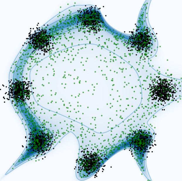
(a) $\lambda=0.1$

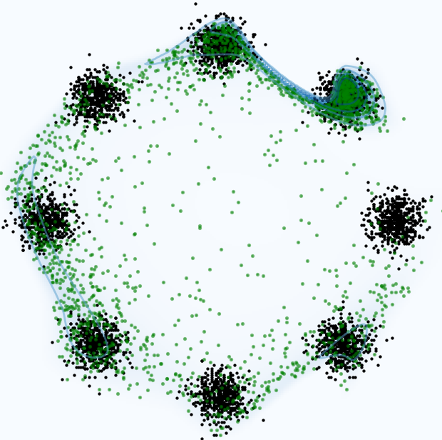
(b) $\lambda=1$

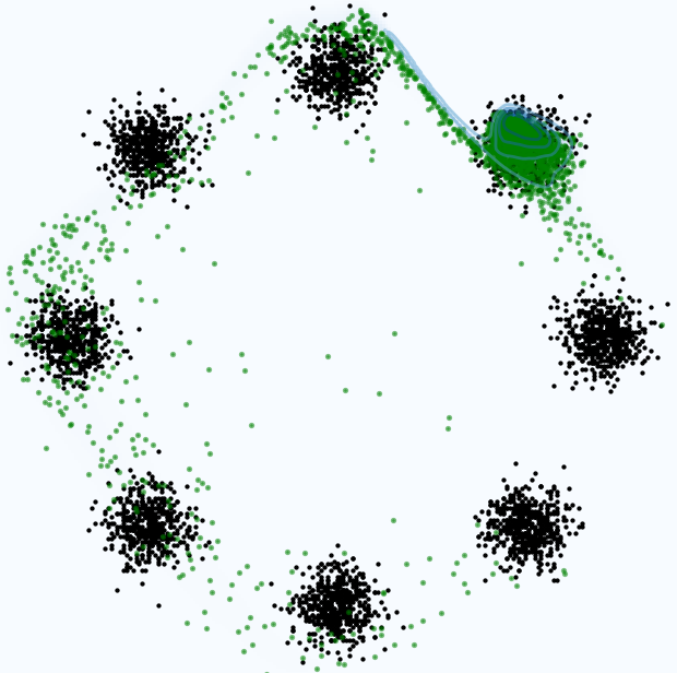
(c) $\lambda=10$

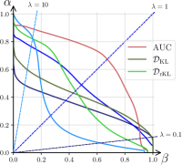
(d) PR Curves

Figure 1: Normalizing Flows (RealNVP) trained on two dimensional data-points sampled from 8 Gaussians. Fig. 1(a) to Fig. 1(c): three models trained to minimise the Precision-Recall Divergence with a different precision/recall trade-off. Samples drawn from the true distribution $P$ are represented in black, samples from trained models $\widehat{P}$ are represented in green, and the log-likelihood of $\widehat{P}$ is represented as the blue levels (darker means higher density). (a) $\lambda=0.1$, favours recall over precision. (b) $\lambda=1$, balanced precision vs. recall trade-off. (c) $\lambda=10$, favours precision over recall. Fig. 1(d): Precision-recall curves of models trained with different divergences. In blue, the three models from Figure 1 (a) to (c). In dark and light green respectively, models trained using $\mathcal{D}_{\mathrm{KL}}$ divergence, and $\mathcal{D}_{\mathrm{rKL}}$. In red, the model has been trained on the AUC. (See also Fig. 5(a), Fig. 5(b) and Fig. 5(c).)

In this paper, we address Questions 1 and 2 by making the following contributions.

• We show that achieving a specified precision-recall trade-off corresponds to minimising a particular f-divergence between $P$ and $\widehat{P}$. Specifically, in Theorem 4.3 we give a family of $f$-divergences (denoted by $\mathcal{D}_{\lambda{\scaleto{\mbox{-}\mathrm{PR}}{0.7ex}}}$, $\lambda\in[0,\infty]$) that are associated with various points along the precision-recall curve of the generative model.

• We show that any arbitrary $f$-divergence can be written as a linear combination of $f$-divergences from the $\mathcal{D}_{\lambda{\scaleto{\mbox{-}\mathrm{PR}}{0.7ex}}}$ family. This result makes explicit, the implicit precision-recall trade-offs made by generative models that minimise an arbitrary $f$-divergence.

• We propose a novel flow-based generative model that can achieve a user specified trade-off between precision and recall by minimising $\mathcal{D}_{\lambda{\scaleto{\mbox{-}\mathrm{PR}}{0.7ex}}}$ for any given $\lambda$.

Figure 1 shows how our model performs under various settings of $\lambda$. With a high $\lambda$, we can train the model to favour precision over recall and vice-versa.

Because the discriminator trained with $\mathcal{D}_{\lambda{\scaleto{\mbox{-}\mathrm{PR}}{0.7ex}}}$ is mostly flat away from the origin, it is not feasible to directly train an $f$-GAN to minimise $\mathcal{D}_{\lambda{\scaleto{\mbox{-}\mathrm{PR}}{0.7ex}}}$ lest we suffer from vanishing gradients. We solve this problem by adversarially training a normalizing flow in conjunction with a discriminator. Our model have the following novelties over existing works.

• The normalizing flow of our model minimises $\mathcal{D}_{\lambda{\scaleto{\mbox{-}\mathrm{PR}}{0.7ex}}}$ instead of the usual $\mathcal{D}_{\mathrm{KL}}$. In fact, one can train a normalizing flow to minimise any $f$-divergence using our scheme.

• To train the discriminator of our model, we use a divergence $\mathcal{D}_{f}$ that is different from $\mathcal{D}_{\lambda{\scaleto{\mbox{-}\mathrm{PR}}{0.7ex}}}$ in order to have stable training without vanishing gradients. This separates our training from the min-max training of GANs and flow-GANs, as we use different loss functions for generator and discriminator. The conditions for compatibility between the two divergences used for training are stated in Theorem 5.3.

Notation:

We use $\mathcal{P}(\mathcal{X})$ to denote the set of probability measures on the space $\mathcal{X}$. We use uppercase letters to denote probability measures and the corresponding lower case letters to denote their density functions. Throughout the paper, we use $\mathcal{X}\subseteq\mathbb{R}^{d}$ for the input space, $P\in\mathcal{P}(\mathcal{X})$ for the target distribution we want to model and $\widehat{P}\in\mathcal{P}(\mathcal{X})$ for the distribution estimated by a generative model. Further, we assume that $P$ and $\widehat{P}$ share the same support in $\mathcal{X}$.

2 Related works

The task of improving Normalizing Flows by tackling the trade-off between the natural effect of mass covering of $\mathcal{D}_{\mathrm{KL}}$ and a desired mode seeking result has been done in some previous work. Reject can be used to artificially improve the precision of a model (Stimper et al., 2022; Issenhuth et al., 2022; Tanielian et al., 2020). But by only focusing on the loss, an approach of Midgley et al. (2022b) trains a Normalizing Flow to minimise an $\alpha$-Divergence for $\alpha=2$, estimated with annealed importance sampling. While the work show the benefits from training with another $f$-divergence, it fixes the trade-off by fixing the $\alpha$. Moreover, their work requires to know the target distribution density $P$ as they aim to train the Flow to be sampler.

To generalise the approach of training a flow on any $f$-divergence divergence in an unsupervised setting, our method relies on the work of Nowozin et al. (2016) for GANs. This framework has been evaluated on Normalizing Flows by Grover et al. (2018). It has been shown that Flows can be trained with a discriminator and that adversarially trained model gain from a log-likelihood terms, however the authors restrain their evaluation to Wasserstein distance only and do not explore how the $f$-divergence affects the Flow.

Moreover, we make the link between $f$-divergences and Precision and Recall. Several works have been trying to evaluate the these values with clustering methods reduced dimension space (Sajjadi et al., 2018; Tanielian et al., 2020; Kynkäänniemi et al., 2019). We use likelihood ratio estimation to compute the metrics like (Simon et al., 2019), but we offer guaranties on the the quality of the estimation. Finally, while we formulate the precision as an $f$-divergence, Djolonga et al. (2020) introduce a different evaluation framework based on Rényi divergences. All theses previous works only focus on the evaluation of the model but we build method to train models based on this metric.

3 Background

3.1 Preliminaries on Normalising Flows

Let $\mathcal{Z}\subseteq\mathbb{R}^{d}$ be a latent space. Let $Q\in\mathcal{P}(\mathcal{Z})$ denote the standard normal distribution, $\mathcal{N}(0,\mathcal{I}_{d})$. Given a target distribution $P\in\mathcal{P}(\mathcal{X})$, one seeks a Normalizing Flow (Rezende & Mohamed, 2016) i.e., a bijection $F:\mathcal{X}\to\mathcal{Z}$ such that $P(A)=Q(F^{-1}(A))$ for any measurable $A\subseteq\mathcal{X}$. One can then use $F$ to generate samples from $P$ by applying $F^{-1}$ to samples from $Q$, or compute the density $p(x)$ for $x\in\mathcal{X}$ using the change of variable formula, $p(\boldsymbol{x})=q(F(\boldsymbol{x}))|\det\mathrm{Jac}_{F}(\boldsymbol{x})|$, where $\det\mathrm{Jac}_{F}(\boldsymbol{x})$ is determinant of Jacobian matrix of $F$ at $\boldsymbol{x}$.

In practice, $F$ is not known, and the goal is to find a mapping $F^{\prime}$ that yields the best approximation $\widehat{P}_{F^{\prime}}$ of $P$. To do so, we consider a class of invertible functions $\{F_{\theta}:\theta\in\Theta\}$ typically represented using invertible neural network (INN) architectures such as GLOW (Kingma & Dhariwal, 2018), RealNVP (Rezende & Mohamed, 2016) or ResFlow (Behrmann et al., 2019; Chen et al., 2020). We can then train the INN to minimise the KL-divergence between $P$ and $\widehat{P}_{F_{\theta}}$, or equivalently, by maximising the log-likelihood $\mathbb{E}_{\boldsymbol{x}\sim P}\left[\log\hat{p}_{F_{\theta}}(\boldsymbol{x})\right]$ estimating using a dataset $D$ of samples from $P$.

$$\begin{split}\min_{\theta}\ &\mathcal{D}_{\mathrm{KL}}(P\|\widehat{P}_{F_{\theta}})=\min_{\theta}\int_{\mathcal{X}}p(\boldsymbol{x})\log\frac{p(\boldsymbol{x})}{\hat{p}_{F_{\theta}}(\boldsymbol{x})}\mathrm{d}\boldsymbol{x}\\ &=H(P)-\max_{\theta}\mathbb{E}_{\boldsymbol{x}\sim P}\left[\log\hat{p}_{F_{\theta}}(\boldsymbol{x})\right],\end{split}$$ (1)

where $H(P)$ is the entropy of $P$. In the rest of this paper, we omit the dependence on $F_{\theta}$ in $\widehat{P}_{F_{\theta}}$ when it is clear from context.

In order to perform well in practice, the INN must satisfy several properties (Kobyzev et al., 2020): the forward pass and the inverse pass must be efficient to compute ; computing the determinant of the Jacobian matrix must be tractable; finally, $\{F_{\theta}:\theta\in\Theta\}$ should be expressive enough to model $P$. While a number of architectures have been introduced to solve the first two properties, expressivity remains a challenge because of the invertibility constraint. As a consequence $\widehat{P}\neq P$ in most practical scenarios, and thus the divergence that is used to measure the distance between $P$ and $\widehat{P}$ has a critical impact on the resulting model.

Table 1: List of usual $f$-divergences. The generator function $f$ is given with its Fenchel Conjugate. The optimal discriminator $T^{\mathrm{opt}}$ is given in order to compute $p(\boldsymbol{x})/\widehat{p}(\boldsymbol{x})$. Then $f^{\prime\prime}(1/\lambda)/\lambda^{3}$ is given to compute the $f$-divergence as combination of Precision-Recall Divergence.

Divergence	Notation	$f(u)$	$f^{*}(t)$	$T^{\mathrm{opt}}(\boldsymbol{x})$	$f^{\prime\prime}(1/\lambda)/\lambda^{3}$
KL	$\mathcal{D}_{\mathrm{KL}}(P\|\widehat{P})$	$u\log u$	$\exp(t-1)$	$1+\log p({\boldsymbol{x}})/\widehat{p}(\boldsymbol{x})$	$1/\lambda^{2}$
Reverse KL	$\mathcal{D}_{\mathrm{rKL}}(P\|\widehat{P})$	$-\log u$	$-1-\log-t$	$-\widehat{p}(\boldsymbol{x})/p(\boldsymbol{x})$	$1/\lambda$
$\chi^{2}$-Pearson	$\mathcal{D}_{\chi^{2}}(P\|\widehat{P})$	$(u-1)^{2}$	$\frac{1}{4}t^{2}+t$	$2\left(p(\boldsymbol{x})/\widehat{p}(\boldsymbol{x})-1\right)$	$2/\lambda^{3}$
Total Variation	$\mathcal{D}_{\mathrm{TV}}$	$|u-1|/2$	$t$	$\mathrm{sign}\left(p(\boldsymbol{x})/\widehat{p}(\boldsymbol{x})-1\right)/2$	NA

3.2 $f$-divergences

Following the work by Nowozin et al. (2016), we consider the family of $f$-divergences to measure the difference between the true distribution $P$ and the estimated distribution $\widehat{P}$. Given a convex lower semi-continuous function $f:\mathbb{R}^{+}\rightarrow\mathbb{R}$ satisfying $f(1)=0$, the $f$-divergence between two probability distributions $P$ and $\widehat{P}$ is defined as follows.

$$\mathcal{D}_{f}(P\|\widehat{P})=\int_{\mathcal{X}}\widehat{p}(\boldsymbol{x})f\left(\frac{p(\boldsymbol{x})}{\widehat{p}(\boldsymbol{x})}\right)\mathrm{d}\boldsymbol{x}.$$ (2)

Many well known statistical divergences such as the Kullback Leibler divergence ($\mathcal{D}_{\mathrm{KL}}$), the reverse Kullback Leibler ($\mathcal{D}_{\mathrm{rKL}}$) or the Total Variation ($\mathcal{D}_{\mathrm{TV}}$) are $f$-divergences (see Table 1). $D_{f}$ also admits a dual variational form (Nguyen et al., 2009).

$$\mathcal{D}_{f}(P\|\widehat{P})=\sup_{T\in\mathcal{T}}\left(\mathbb{E}_{P}\left[T(\boldsymbol{x})\right]-\mathbb{E}_{\widehat{P}}\left[f^{*}(T(\boldsymbol{x}))\right]\right),$$ (3)

where $\mathcal{T}$ is the set of measurable functions $\mathcal{X}\to\mathbb{R}$ and $f^{*}:\mathbb{R}\to\mathbb{R}$ is the convex conjugate (or Fenchel transform) of $f$ given by $f^{*}(t)=\sup_{u\in\mathbb{R}}\left\{tu-f(u)\right\}$. We use $T^{\mathrm{opt}}\in\mathcal{T}$ to denote the function that achieves the supremum in (3).

Defining,

$$\mathcal{D}^{\mathrm{dual}}_{f,T}(P\|\widehat{P})=\mathbb{E}_{\boldsymbol{x}\sim P}\left[T(\boldsymbol{x})\right]-\mathbb{E}_{\boldsymbol{x}\sim\widehat{P}}\left[f^{*}(T(\boldsymbol{x}))\right],$$ (4)

it is possible to train a generative model for $P$ by solving $\min_{F}\max_{T}\mathcal{D}^{\mathrm{dual}}_{f,T}(P\|\widehat{P})$, where $F$ and $T$ are represented by a neural network (Nowozin et al., 2016).

3.3 Precision-Recall curve for generative models

Typically, generative models are evaluated by a one-dimensional metric like the Inception Score (Salimans et al., 2016) or the Fréchet Inception Distance (Heusel et al., 2017), which are unable to distinguish between the distinct failure modes of low precision (i.e. failure to produce quality samples) and low recall (i.e. failure to cover all modes of $P$). The following definition introduced by Sajjadi et al. (2018) and later extended by Simon et al. (2019) remedies this problem.

Definition 3.1 (PRD set, adapted from Simon et al. (2019)).

For $P,\widehat{P}\in\mathcal{P}(\mathcal{X})$, the Precision-Recall set $\mathrm{PRD}(P,\widehat{P})$ is defined as the set of Precision-Recall pairs $(\alpha,\beta)\in\mathbb{R}^{+}~{}\times~{}\mathbb{R}^{+}$ such that there exists $\mu\in\mathcal{P}(\mathcal{X})$ for which $P\geq\beta\mu$ and $\widehat{P}\geq\alpha\mu$. The precision-recall curve (or PR curve) is defined as $\partial\mathrm{PRD}(P,\widehat{P})=\{(\alpha,\beta)\in\mathrm{PRD}(P,\widehat{P})\mid\nexists(\alpha^{\prime},\beta^{\prime})\mbox{ with }\alpha^{\prime}\geq\alpha\mbox{ and }\beta^{\prime}\geq\beta\}$.

Sajjadi et al. (2018) show that the PR curve is parametrised by $\lambda\in\mathbb{R}^{+}\cup \{+\infty\}$ as follows:

$$\begin{split}&\partial\mathrm{PRD}(P,\widehat{P})=\left\{\alpha_{\lambda}(P\|\widehat{P}),\beta_{\lambda}(P\|\widehat{P})~{}|~{}\lambda\in\mathbb{R}^{+}\cup \{+\infty\}\right\}\\ &\quad\mbox{with }\begin{cases}\alpha_{\lambda}(P\|\widehat{P})=\int_{\mathcal{X}}\min\left(\lambda p(\boldsymbol{x}),\widehat{p}(\boldsymbol{x})\right)\mathrm{d}\boldsymbol{x},\\ \beta_{\lambda}(P\|\widehat{P})=\int_{\mathcal{X}}\min\left(p(\boldsymbol{x}),\widehat{p}(\boldsymbol{x})/\lambda\right)\mathrm{d}\boldsymbol{x}.\end{cases}\end{split}$$ (5)

Note that $\beta_{\lambda}(P\| \widehat{P})=\alpha_{\lambda}(P\| \widehat{P})/\lambda$. We call $\lambda$ the trade-off parameter since it can be used to adjust the sensitivity to precision (or recall). An illustration of the PR curve is given in Figure 2 for a target distribution $P$ that is a mixture of two Gaussians, and two candidate models $\widehat{P}_{1}$ and $\widehat{P}_{2}$. We can see on Figure 2 that $\widehat{P}_{1}$ offers better results for large values of $\lambda$ (with high sensitivity to precision) whereas $\widehat{P}_{2}$ offers better results for low values of $\lambda$ (with high sensitivity to recall).

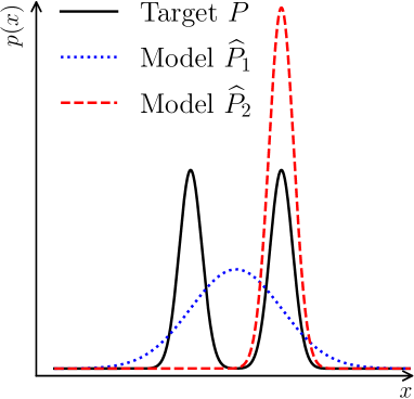
(a) Distributions

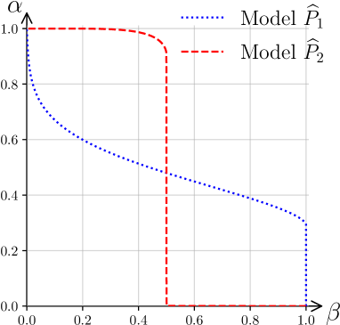
(b) $\partial\mathrm{PRD}(P,\widehat{P})$ curves

Figure 2: PR curves for two models $\widehat{P}_{1}$ and $\widehat{P}_{2}$ of $P$. Figure 2(a) shows $\widehat{P}_{1},\widehat{P}_{2}$ and $P$. Figure 2(a) shows PR curves for $\widehat{P}_{1},\widehat{P}_{2}$ against $P$. $\widehat{P}_{1}$ has good recall since it covers both modes of $P$ but low precision since it generates points between the modes. $\widehat{P}_{2}$ has good precision since it does not generate samples outside of $P$ but low recall since it can generate samples from only one mode.

4 Precision and Recall trade-off as a $f$-divergence

In this section, we formalise the link between precision-recall trade-off and $f$-divergences, and address Question 1. We will exploit this link in Section 5 to train models that optimise a particular trade-off between precision and recall.

4.1 Precision-Recall as an $f$-divergence

We start by introducing the PR-Divergence as follows.

Definition 4.1 (PR-divergence).

Given a trade-off parameter $\lambda\in\mathbb{R}^{+}\cup+\infty$, the PR-divergence (denoted by $\mathcal{D}_{\lambda{\scaleto{\mbox{-}\mathrm{PR}}{0.7ex}}}$) is defined as the $f_{\lambda}$-divergence for $f_{\lambda}:\mathbb{R}^{+}\to\mathbb{R}$ defined as

$$f_{\lambda}:u\mapsto\max(\lambda u,1)-\max(\lambda,1),$$

for $\lambda\in\mathbb{R}^{+}$ and $f_{\lambda}:u\mapsto 0$ for $\lambda=+\infty$.

Note that $f_{\lambda}$ is continuous, convex, and satisfies $f_{\lambda}(1)=0$ for all $\lambda$. A graphical representation of $f_{\lambda}$ can be found in Appendix  A.2. The following proposition gives some properties of $\mathcal{D}_{\lambda{\scaleto{\mbox{-}\mathrm{PR}}{0.7ex}}}$.

Proposition 4.2 (Properties of the PR-Divergence).

• The Fenchel conjugate $f_{\lambda}^{*}$ of $f_{\lambda}$ is defined on $\mathrm{dom}\left(f_{\lambda}^{*}\right)=\left[0,\lambda\right]$ and given by,

  $$f_{\lambda}^{*}\left(t\right)=\begin{cases}t/\lambda&\mbox{ if }\,\lambda\leq 1,\\ t/\lambda+\lambda-1&\mbox{otherwise.}\end{cases}$$ (6)

• The discriminator $T^{\mathrm{opt}}$ that achieves the supremum in the variational representation of $\mathcal{D}_{\lambda{\scaleto{\mbox{-}\mathrm{PR}}{0.7ex}}}(P\|\widehat{P})$ is

  $$T^{\mathrm{opt}}(\boldsymbol{x})=\lambda\mathrm{sign}\left\{\frac{p(\boldsymbol{x})}{\widehat{p}(\boldsymbol{x})}-1\right\}.$$ (7)

• $\mathcal{D}_{\lambda{\scaleto{\mbox{-}\mathrm{PR}}{0.7ex}}}(\widehat{P}\|P)=\lambda\mathcal{D}_{\frac{1}{\lambda}{\scaleto{\mbox{-}\mathrm{PR}}{0.7ex}}}(P\|\widehat{P})$.

• $\mathcal{D}_{1{\scaleto{\mbox{-}\mathrm{PR}}{0.7ex}}}(P\|\widehat{P})=\mathcal{D}_{\mathrm{TV}}(P\|\widehat{P})/2$.

Having defined the PR-divergence, we can now show that precision and recall w.r.t $\lambda$ can be expressed as a function of the divergence between $P$ and $\widehat{P}$.

Theorem 4.3 (Precision and recall as a function of $\mathcal{D}_{\lambda{\scaleto{\mbox{-}\mathrm{PR}}{0.7ex}}}$).

Given $P,\widehat{P}\in\mathcal{P}(\mathcal{X})$ and $\lambda\in\mathbb{R}^{+}\cup\{+\infty\}$, the PR curve $\partial\mathrm{PRD}(P,\widehat{P})$ is related to the PR-divergence $\mathcal{D}_{\lambda{\scaleto{\mbox{-}\mathrm{PR}}{0.7ex}}}(P\|\widehat{P})$ as follows.

$$\alpha_{\lambda}(P\| \widehat{P}) =\min(1,\lambda)-\mathcal{D}_{\lambda{\scaleto{\mbox{-}\mathrm{PR}}{0.7ex}}}(P\|\widehat{P}).$$ (8)

A direct consequence of Theorem 4.3 is that we can now train the parameters of a model $F_{\theta}$ to maximise precision and recall by minimising the corresponding PR-divergence.

$$\operatorname*{argmax}_{\theta}~{}\alpha_{\lambda}(P\|\widehat{P}_{F_{\theta}})=\operatorname*{argmin}_{\theta}~{}\mathcal{D}_{\lambda{\scaleto{\mbox{-}\mathrm{PR}}{0.7ex}}}(P\|\widehat{P}_{F_{\theta}}).$$ (9)

In other terms, training a model to minimise $\mathcal{D}_{\lambda{\scaleto{\mbox{-}\mathrm{PR}}{0.7ex}}}$ means that the model will specifically focus the set trade-off. One might wonder what is the trade-off, ie the function $a_{\lambda}$ minimised when the model is trained on the $\mathcal{D}_{\mathrm{KL}}$.

4.2 Relation between PR-divergences and other $f$-divergences

In the previous subsection, we showed that for each trade-off parameter $\lambda$, there exists an $f$-divergence that corresponds to optimising for it. This raises the converse question of what trade-off is achieved by optimizing for an arbitrary $f$-divergence. We answer this by showing in the following theorem that any $f$-divergence can be expressed as a weighted sum of PR-divergences.

Theorem 4.4 ($f$-divergence as weighted sums of PR-divergences).

For any $P,\widehat{P}\in\mathcal{P}(\mathcal{X})$ supported on all of $\mathcal{X}$ and any $\lambda\in\mathbb{R}^{+}$,

$$\mathcal{D}_{f}(P\|\widehat{P})=\int^{M}_{m}\frac{1}{\lambda^{3}}f^{\prime\prime}\left(\frac{1}{\lambda}\right)\mathcal{D}_{\lambda{\scaleto{\mbox{-}\mathrm{PR}}{0.7ex}}}(P\|\widehat{P})\mathrm{d}\lambda,$$ (10)

where $m=\min_{\mathcal{X}}\left(\frac{\widehat{p}(\boldsymbol{x})}{p(\boldsymbol{x})}\right)$ and $M=\max_{\mathcal{X}}\left(\frac{\widehat{p}(\boldsymbol{x})}{p(\boldsymbol{x})}\right)$.

Combining Theorem 4.4 with Theorem 4.3 we have the following relation that captures the implicit precision-recall trade-off made by minimising an arbitrary $f$-divergence.

$$\operatorname*{argmin}_{\theta}\mathcal{D}_{f}(P\|\widehat{P})=\operatorname*{argmax}_{\theta}\int_{m}^{M}\frac{1}{\lambda^{3}}f^{\prime\prime}\left(\frac{1}{\lambda}\right)\alpha_{\lambda}(P\|\widehat{P})\mathrm{d}\lambda,$$ (11)

In the following corollary, we apply Theorem 4.4 to compare $\mathcal{D}_{\mathrm{KL}}$ and $\mathcal{D}_{\mathrm{rKL}}$.

Corollary 4.5 ($\mathcal{D}_{\mathrm{KL}}$ and $\mathcal{D}_{\mathrm{rKL}}$ as an average of $\mathcal{D}_{\lambda{\scaleto{\mbox{-}\mathrm{PR}}{0.7ex}}}$).

The $\mathcal{D}_{\mathrm{KL}}$ Divergence and the $\mathcal{D}_{\mathrm{rKL}}$ can be written as weighted average of PR-Divergence $\mathcal{D}_{\lambda{\scaleto{\mbox{-}\mathrm{PR}}{0.7ex}}}$:

$$\mathcal{D}_{\mathrm{KL}}(P\|\widehat{P})=\int_{m}^{M}\frac{1}{\lambda^{2}}\mathcal{D}_{\lambda{\scaleto{\mbox{-}\mathrm{PR}}{0.7ex}}}(P\|\widehat{P})\mathrm{d}\lambda,$$ (12)

$$\mathcal{D}_{\mathrm{rKL}}(P\|\widehat{P})=\int_{m}^{M}\frac{1}{\lambda}\mathcal{D}_{\lambda{\scaleto{\mbox{-}\mathrm{PR}}{0.7ex}}}(P\|\widehat{P})\mathrm{d}\lambda.$$ (13)

As we can see in this Corollary, both $\mathcal{D}_{\mathrm{KL}}$ and $\mathcal{D}_{\mathrm{rKL}}$ can be decomposed into a sum of PR-divergences terms $\mathcal{D}_{\lambda{\scaleto{\mbox{-}\mathrm{PR}}{0.7ex}}}$, each weighted with $1/\lambda^{2}$ and $1\lambda$ respectively. Hence $\mathcal{D}_{\mathrm{KL}}$ gives more weight to small $\lambda$ (more sensitive to precision) than $\mathcal{D}_{\mathrm{rKL}}$. This explains the mode covering behaviour observed in Normalizing Flows trained with $\mathcal{D}_{\mathrm{KL}}$. Comparatively, the $\mathcal{D}_{\mathrm{rKL}}$ assigns more weight to terms with a large lambda and less weight to the terms with a small lambda, leading to the mode covering behaviour empirically observed with flows trained with the $\mathcal{D}_{\mathrm{rKL}}$ (Midgley et al., 2022a).

5 Optimising for specific Precision-Recall trade-offs

In this section, we address Question 2 by proposing a model that achieves a specified precision-recall trade-off. In light of Theorem 4.3, a natural approach would be to use the framework of Nowozin et al. (2016) and train an $f_{\lambda}$-GAN to minimize the dual variational form of $\mathcal{D}_{\lambda{\scaleto{\mbox{-}\mathrm{PR}}{0.7ex}}}$ for any given $\lambda$, as follows.

$$\min_{F}\max_{T}\mathcal{D}^{\mathrm{dual}}_{f_{\lambda},T}(P\|\widehat{P})$$

$$=\min_{F}\max_{T}\mathbb{E}_{\boldsymbol{x}\sim P}\left[T(\boldsymbol{x})\right]-\mathbb{E}_{\boldsymbol{x}\sim\widehat{P}}\left[f^{*}_{\lambda}(T(\boldsymbol{x}))\right],$$

where both $F$ and $T$ are parametrized by neural networks. As noted in Nowozin et al. (2016), we need to use an output activation function $\sigma_{\lambda}$ on $T(x)$ so that $\sigma(T(x))\in dom(f_{\lambda}^{*})$. From Proposition 4.2, we have that the domain of $f^{*}_{\lambda}$ is bounded (equal to $[0,\lambda]$) unlike most other popular $f$-divergences including $\mathcal{D}_{\mathrm{KL}}$ and $rKL$, $\chi^{2}$, Jensen-Shannon and Hellinger, except for the case of Total Variation. Due to this, we are forced to choose an output activation function like the sigmoid that suffers from vanishing gradients. Because of this, we find that $f_{\lambda}$-GAN is notoriously hard to train and performs poorly, not unlike the case of training $f$-GAN with the Total Variation metric.

We overcome this problem by using the primal form of $f$-divergence shown in (2) to minimise $\mathcal{D}_{\lambda{\scaleto{\mbox{-}\mathrm{PR}}{0.7ex}}}$ rather than the dual variational form in (3), as explained in the following subsection.

5.1 Minimising the primal estimation of $\mathcal{D}_{\lambda{\scaleto{\mbox{-}\mathrm{PR}}{0.7ex}}}$

Figure 3: Model architecture for training a Normalising Flow $F$ that minimises $\mathcal{D}_{g}$ using a discriminator $T$ that minimises $\mathcal{D}_{f}$.

As explained before, using the the $f$-GAN approach to minimise the dual variational form of $\mathcal{D}_{\lambda{\scaleto{\mbox{-}\mathrm{PR}}{0.7ex}}}$ is not a feasible approach. In this subsection, we introduce a novel approach to instead train a Normalizing Flow to minimise $\mathcal{D}_{\lambda{\scaleto{\mbox{-}\mathrm{PR}}{0.7ex}}}$. We do this by using the primal form of $f$-divergence, given by $\mathcal{D}_{f}(P\|\widehat{P})=\int_{\mathcal{X}}\widehat{p}(\boldsymbol{x})f\left(\frac{p(\boldsymbol{x})}{\widehat{p}(\boldsymbol{x})}\right)\mathrm{d}\boldsymbol{x}$. Computing $D_{f}$ with the primal form requires the likelihood ratio $p(x)/\widehat{p}(x)$. For this, we use the $T^{\mathrm{opt}}$ from the dual form of $D_{f}$. From the dual form, we have the following.

$$\mathcal{D}_{f}(P\|\widehat{P})=\sup_{T\in\mathcal{T}}\int_{\mathcal{X}}\left(p(x)T(x)-\widehat{P}(x)f^{*}(T(x))\right)dx.$$

Differentiating the expression inside the integral with respect to $T(x)$, we get the following.

$$\frac{p(x)}{\widehat{p}(x)}=\nabla f^{*}(T^{\mathrm{opt}}(x)).$$ (14)

We use the preceding equation to propose the following definition for a primal estimate of $f$-divergence.

Definition 5.1 (Primal estimate $\mathcal{D}^{\mathrm{primal}}_{g,T}$).

Let $P,\widehat{P}\in\mathcal{P}(\mathcal{X})$. For functions $T:\mathcal{X}\to\mathbb{R}$ and $f,g:\mathbb{R}^{+}\to\mathbb{R}$, we define the primal estimate $\mathcal{D}^{\mathrm{primal}}_{g,T}$ of the divergence $\mathcal{D}_{g}$ as follows.

$$\mathcal{D}^{\mathrm{primal}}_{g,T}(P\|\widehat{P})=\int_{\mathcal{X}}\widehat{p}(\boldsymbol{x})g\left(r(\boldsymbol{x})\right)\mathrm{d}\boldsymbol{x},$$ (15)

where $r:\mathcal{X}\rightarrow\mathbb{R}^{+}$ is given by, $r(\boldsymbol{x})=\nabla f^{*}(T(\boldsymbol{x}))$.

Crucially, when $T^{\mathrm{opt}}$ is as given in (14), we have $\mathcal{D}^{\mathrm{primal}}_{g,T}=\mathcal{D}_{g}$. Also note that $r(x)$ acts as the estimate for the likelihood $p(x)/\widehat{p}(x)$. With this, we propose the following scheme for training a Normalizing Flow $F$ that minimises $\mathcal{D}_{g}$ by using a discriminator $T$ that minimises $\mathcal{D}_{f}$.

• The discriminator $T$ is trained to minimise $\mathcal{D}_{f}$ with the dual variational form.

  $$\operatorname*{argmin}_{T}\mathcal{D}^{\mathrm{dual}}_{f,T}(P\|\widehat{P})$$

  $$=\operatorname*{argmin}_{T}\mathbb{E}_{P}\left[T(\boldsymbol{x})\right]-\mathbb{E}_{\widehat{P}}\left[f^{*}(T(\boldsymbol{x}))\right].$$

• The generator, a Normalizing Flow $F$, is trained to maximise $\mathcal{D}_{g}$ with the primal form.

  $$\operatorname*{argmin}_{T}\mathcal{D}^{\mathrm{primal}}_{g,T}$$

  $$=\operatorname*{argmin}_{T}\mathbb{E}_{\widehat{P}}\left[g(\nabla f^{*}(T(\boldsymbol{x})))\right].$$

Note that for $T=T^{\mathrm{opt}}$, we have $\mathcal{D}^{\mathrm{dual}}_{f,T}(P\|\widehat{P})=\mathcal{D}_{f}$, and consequently, $\mathcal{D}^{\mathrm{primal}}_{g,T}=\mathcal{D}_{g}$. Figure 3 shows the model architecture and Algorithm 1 depicts the training process.

Finally, in order to train a generator to minimise $\mathcal{D}_{\lambda{\scaleto{\mbox{-}\mathrm{PR}}{0.7ex}}}$, we use $g=f_{\lambda}$ and an $f$ for which $dom(f^{*})$ is not bounded, for example $KL$ or $rKL$ or Jensen-Shannon divergence. In the following subsection, we discuss how the choice of $f$ affects the model training.

Algorithm 1 Training

  Input: Flow $F$, Discriminator $T$, Dataset $D$

  for  epoch $e=1,\dots,E$ do

     $\mathcal{L}_{d},\mathcal{L}_{p}\leftarrow 0,0$

     for $\boldsymbol{x}_{\mathrm{real}}\in D$ do

        Generate $\boldsymbol{x}_{\mathrm{fake}}=F^{-1}(\boldsymbol{z})$ with $\boldsymbol{z}\sim\mathcal{N}(\boldsymbol{0}_{d},\boldsymbol{I}_{d})$

        $\mathcal{L}_{d}\leftarrow\mathcal{L}_{d}+T(\boldsymbol{x}_{\mathrm{real}})-f^{*}(T(x_{\mathrm{fake}}))$

        $\mathcal{L}_{d}\leftarrow\mathcal{L}_{d}+g\left(\nabla f^{*}(T(\boldsymbol{x}_{\mathrm{fake}})\right)$

     end for

     Update $T$ to maximise $\mathcal{L}_{d}$

     Update $F$ to minimise $\mathcal{L}_{p}$

  end for

5.2 Choosing the right $f$ to train T

To use the proposed model for optimizing for PR-divergences, we fix $g=f_{\lambda}$. This still leaves us with the flexibility to choose $f$ for which $dom(f^{*})$ is not bounded. The choice of $f$ affects the estimate $r(x)=\nabla f^{*}(T(x))$ of the likelihood $p(x)/\widehat{p}(x)$. In the following theorem, we show that the Bregman divergence associated with $f$ place a crucial role in the goodness of approximation of the dual form $\mathcal{D}^{\mathrm{dual}}_{f,T}(P\|\widehat{P})$.

Theorem 5.2 (Error of the estimation of an $f$-divergence under the dual form.).

For any discriminator $T:\mathcal{X}\rightarrow\mathbb{R}$ and $r\left(\boldsymbol{x}\right)=\nabla f^{*}(T(\boldsymbol{x}))$,

$$D_{f}(P\|\widehat{P})-D_{f,T}^{\mathrm{dual}}(P\|\widehat{P})=\mathbb{E}_{\widehat{P}}\left[\mathrm{Breg}_{f}\left(r(\boldsymbol{x}),\frac{p(\boldsymbol{x})}{\widehat{p}(\boldsymbol{x})}\right)\right].$$ (16)

In the next theorem, we bound the approximation error of $\mathcal{D}_{g,T}^{\mathrm{primal}}(P\|\widehat{P})$.

Theorem 5.3 (Bound on the estimation of an $f$-divergence using another $f$-divergence).

Let $f,g:\mathbb{R}^{+}\to\mathbb{R}$ be such that $f$ is $\mu$-strongly convex and $g$ is $\sigma$-Lipschitz. For discriminator $T:\mathcal{X}\rightarrow\mathbb{R}$, let $r\left(\boldsymbol{x}\right)=\nabla f^{*}(T(\boldsymbol{x}))$. If

$$\mathcal{D}_{f}(P\|\widehat{P})-\mathcal{D}^{\mathrm{dual}}_{f,T}(P\|\widehat{P})\leq\epsilon,$$

then,

$$\left|\mathcal{D}_{g}(P\|\widehat{P})-\mathcal{D}_{g,T}^{\mathrm{primal}}(P\|\widehat{P})\right|\leq\sigma\sqrt{\frac{2\epsilon}{\mu}}.$$

Note that $g=f_{\lambda}$ is indeed Lipschitz for any $\lambda$, and $\mathcal{D}_{f}$ can be chosen so that $f$ is strongly convex (for example, the $\chi^{2}$ divergence). Hence, Theorems 5.2 and 5.3 together provide theoretical support for the convergence of our proposed model. In Figure 4, we show empirical evidence for the convergence of primal and dual forms.

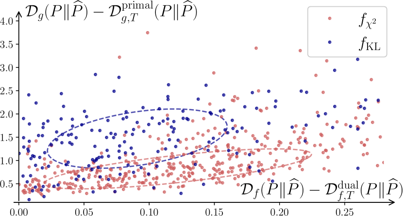
Figure 4: 200 different $P$ and $\widehat{P}$ composed of a mixture of 15 Gaussians have been used to train two discriminators: one on $\mathcal{D}_{\mathrm{KL}}$ and one on $\mathcal{D}_{\chi^{2}}$. For each discriminator, the distance between $\mathcal{D}_{g}$ and its primal and, the distance between $\mathcal{D}_{f}$ and its dual have been reported. The lower the point is on the $y$-axis, the better the estimation is. The red dots are discriminators train with $f_{\chi^{2}}$ and in blue with $f_{\mathrm{KL}}$. The ellipsoid represent the Mahalanobis of each set.

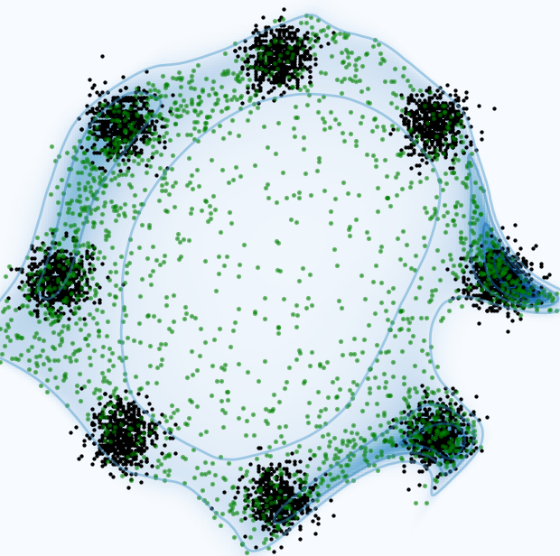
(a) $\mathcal{D}_{\mathrm{KL}}$

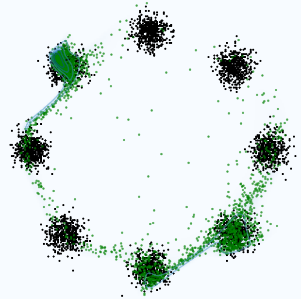
(b) $\mathcal{D}_{\mathrm{rKL}}$

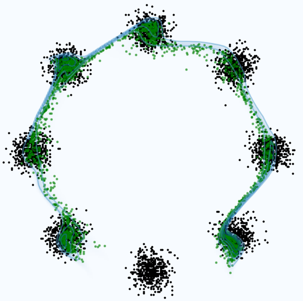
(c) AUC

Figure 5: RealNVP trained on a two dimensional 8 Gaussians Mixtures. Samples from $P$ are represented in black while samples drawn from $\widehat{P}$ are green. The log-likelihood of $\widehat{P}$ is represented as the blue levels, the darker the higher. The models have been trained to minimise (from left to right) the $\mathcal{D}_{\mathrm{KL}}$, the $\mathcal{D}_{\mathrm{rKL}}$ and the Aera Under the Curve (AUC). The corresponding PR-curves are plotted in Figure 1(d).

6 Practical considerations

6.1 A new approach to compute $\partial\mathrm{PRD}(P,\widehat{P})$

To evaluate our model, the frontier $\partial\mathrm{PRD}(P,\widehat{P})$ must be computed. The original work of Sajjadi et al. (2018) proposes a clustering method to estimate every point $\left(\alpha(\lambda),\beta(\lambda)\right)$ but was proven to fail estimate packed data points (Kynkäänniemi et al., 2019). A more recent approach (Simon et al., 2019) proposed to train a binary classifier to make the difference between points from $P$ and $\widehat{P}$ and then use false positive and false negative ratios to estimate the frontier. Since we have proven that the frontier can be estimated by the primal of $\mathcal{D}_{\lambda{\scaleto{\mbox{-}\mathrm{PR}}{0.7ex}}}$ and this for every $\lambda\in\mathbb{R}^{+}$, we can simply use the estimated ratio $\frac{p(\boldsymbol{x})}{p(\boldsymbol{x})}$ obtained with the Discriminator $T$. Therefore, with $r(\boldsymbol{x})=\nabla f^{*}(T(\boldsymbol{x}))$ as the estimated ratio, the estimated precision on the frontier can be written as. By using $\mathcal{D}_{\chi^{2}}$ to train $T$, we certify a bounded error on the estimated precision in opposition to the crossentropy (i.e $\mathcal{D}_{\mathrm{KL}}$) used in the previous approach.

6.2 Training for optimal AUC

Inspired by the work from classification, we can compute and even train the model to optimise the Area Under the Curve (AUC). This will result in a model that achieve good performance across the entire range of possible trade-off values $\lambda$ instead of maximising the performance for one particular trade-off. The AUC can be computed with its expression given in Proposition 6.1 and the model can be trained on this loss.

Proposition 6.1 (AUC under the $\partial\mathrm{PRD}(P,\widehat{P})$).

The aera under the curve is:

$$\mathrm{AUC}=\int_{0}^{+\infty}\alpha_{\lambda}(P\|\widehat{P})^{2}\mathrm{d}\lambda$$ (17)

7 Experiments

In this section, we report on a series of experiments conducted to illustrate the benefits of using the PR-divergence. A first series of experiments is conducted on a 2D dataset (8 gaussians) and the other uses higher dimensional image datasets, MNIST and CelebA. We train RealNVPs (Rezende & Mohamed, 2016) for the first dataset and GLOW (Kingma & Dhariwal, 2018) for the high dimensional datasets. For every model, the discriminator $T$ is trained to maximise $\mathcal{D}_{\chi^{2}}^{\mathrm{dual}}(P\|\widehat{P})$, then the models are trained to minimise different losses estimated with $T$ as described in Section 5.1.

8 Gaussian dataset

Figures 1(a), 1(b) and 1(c) present models trained on the 8 Gaussians dataset, with $\mathcal{D}_{\lambda{\scaleto{\mbox{-}\mathrm{PR}}{0.7ex}}}$ using $\lambda=0.1$, $\lambda=1$ and $\lambda=10$. As we can see, increasing $\lambda$ dramatically improves precision at the cost of recall and vice-versa. Figure 5(a), 5(b) and 5(c), presents models that have been trained to minimise respectively $\mathcal{D}_{\mathrm{KL}}$, $\mathcal{D}_{\mathrm{rKL}}$ and the AUC. The mass covering and the mode seeking behaviours of $\mathcal{D}_{\mathrm{KL}}$ and $\mathcal{D}_{\mathrm{rKL}}$ are clearly demonstrated on this figures. Notice however, that thanks to the flexibility of the PR-divergence, adjust $\lambda$ and choose every model in between these extreme behaviours.

The corresponding PR-curves are plotted in Figure 5. The two green curves are the frontier $\partial\mathrm{PRD}(P,\widehat{P})$ for the $\mathcal{D}_{\mathrm{KL}}$ and the $\mathcal{D}_{\mathrm{rKL}}$ and can be set as the reference. For $\lambda=1$, the model is in between both curves, worse recall than $\mathcal{D}_{\mathrm{KL}}$ and worse precision than $\mathcal{D}_{\mathrm{rKL}}$ but has a better precision than $\mathcal{D}_{\mathrm{KL}}$ and a better recall than $\mathcal{D}_{\mathrm{rKL}}$. With the high value of $\lambda$, we have set a relatively high importance on the precision, and the model performs better than $\mathcal{D}_{\mathrm{rKL}}$ in terms of precision. Finally, the AUC model is not always as good as more specialised models, but has the best AUC and the best $\mathcal{D}_{\mathrm{TV}}$.

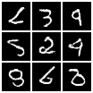
(a) $\lambda=\frac{1}{5}$

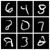
(b) $\lambda=1$

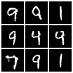
(c) $\lambda=5$

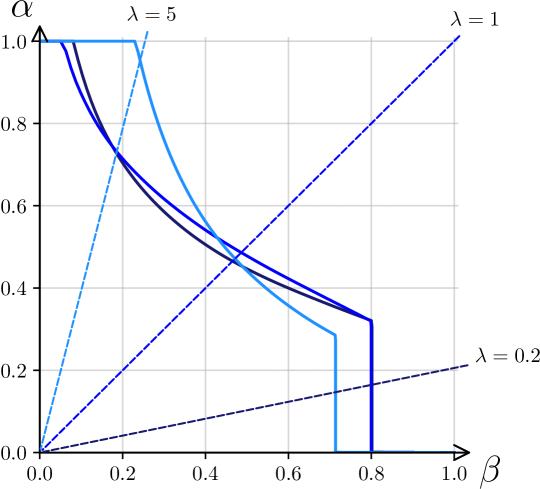
(d) PR-curves

Figure 6: Glow models trained on MNIST. Small batches of samples are given for the different models.

MNIST and CelebA

To test the framework on high dimensional image dataset, we have trained different multi-scale Glow models on the dataset MNIST (Yann LeCun et al., 2010) and a CelebA $64\small{\times}64$ (Liu et al., 2015). Three models for each data set have trained minimising $\mathcal{D}_{\lambda{\scaleto{\mbox{-}\mathrm{PR}}{0.7ex}}}$ with $\lambda=1/5$, $\lambda=1$ and $\lambda=5$. Samples of generated images are showed in Figure 6 for MNIST and Figure 7. (Larger batches are available in Appendix B.) For MNIST, we can see that for values of $\lambda\leq 1$, the generate images have a poor quality and it is represented on the PR-curve as both curves quickly decrease. However, the samples for the model trained with $\lambda=10$ generates samples with low variance (mostly from class $1$, $9$ $8$, $6$ and $4$) but with a better quality. The PR-curve is thus greater for high values of $\lambda$ and lower for low values of $\lambda$. On CelebA, most normalizing flows have trouble generating quality samples with various background. Here we can see that by setting the trade-off on recall, the model generates a wide spectrum of background but with poor quality faces. On the contrary, by setting the trade-off on precision, the model standardise the and improve the precision on the faces.

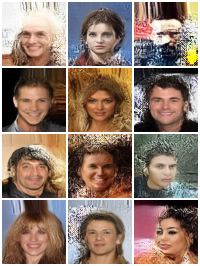
(a) $\lambda=\frac{1}{5}$

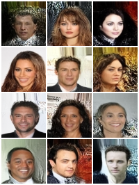
(b) $\lambda=1$

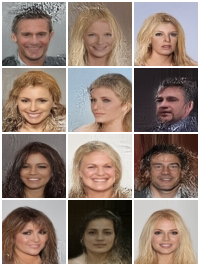
(c) $\lambda=5$

Figure 7: Glow models trained on MNIST. Small batches of samples are given for the different models.

8 Conclusion

In this paper, we present a method for training Normalizing Flows using a new Precision/Recall (PR) divergence within the framework of f-divergences. Our approach offers a unique advantage over other divergences as it allows for explicit control of the precision-recall trade-off in generative models. The PR-divergence results in models that range from extreme mode seeking (high precision) to extreme weight covering (high recall), as well as more balanced models that may be more suitable for various applications. Our framework also provides new insights into other well-known divergences, such as the KL and reverse KL. Our experiments indicate that models trained for high precision (using the reverse KL) often have high precision but poor recall. Given that detecting low recall in a model is more difficult than detecting low precision through visual inspection of model samples, we suspect that existing evaluation methodologies have overemphasised high precision models. As such, we hope that this research will ultimately lead to the development of better tools for evaluating the overall quality of generative models.

Appendix A Appendix A.

A.1 Proof for Theorem 4.3

We have to prove that $\alpha(\lambda)$ can be written as a function of an $f$-divergence for any $\lambda\in\mathbb{R}^{+}$. First we can develop the expression of $\alpha(\lambda)$:

$$\alpha(\lambda) =\int_{\mathcal{X}}\min\left(\lambda p(\boldsymbol{x}),\widehat{p}(\boldsymbol{x})\right)\mathrm{d}\boldsymbol{x}$$ (18)

$$=\int_{\mathcal{X}}\widehat{p}(\boldsymbol{x})\min\left(\lambda\frac{p(\boldsymbol{x})}{\widehat{p}(\boldsymbol{x})},1\right)\mathrm{d}\boldsymbol{x}$$ (19)

For this integral to be considered as an $f$-divergence, we need $f$ to be first convex lower semi-continuous and then to satisfy $f(1)=0$. However, for every $a,b\in\mathbb{R}$, the $\min$ satisfies $\min(a,b)=a+b-\max(a,b)$. Therefore,

$$\alpha(\lambda) =\int_{\mathcal{X}}\widehat{p}(\boldsymbol{x})\left[\lambda\frac{p(\boldsymbol{x})}{\widehat{p}(\boldsymbol{x})}+1-\max\left(\lambda\frac{p(\boldsymbol{x})}{\widehat{p}(\boldsymbol{x})},1\right)\right]\mathrm{d}\boldsymbol{x}$$ (20)

$$=\lambda\int_{\mathcal{X}}p(\boldsymbol{x})\mathrm{d}\boldsymbol{x}+1-\int_{\mathcal{X}}\max\left(\lambda\frac{p(\boldsymbol{x})}{\widehat{p}(\boldsymbol{x})},1\right)\mathrm{d}\boldsymbol{x}$$ (21)

$$=\lambda+1-\int_{\mathcal{X}}\widehat{p}(\boldsymbol{x})\max\left(\lambda\frac{p(\boldsymbol{x})}{\widehat{p}(\boldsymbol{x})},1\right)\mathrm{d}\boldsymbol{x}$$ (22)

Thus, we can take $f(u)=\max(\lambda u,1)-\max(\lambda,1)$ such that $f(1)=0$. The precision becomes:

$$\alpha(\lambda) =\lambda+1-\int_{\mathcal{X}}\widehat{p}(\boldsymbol{x})f(\left(\frac{p(\boldsymbol{x})}{\widehat{p}(\boldsymbol{x})}\right)-\max(\lambda,1)\int_{\mathcal{X}}\widehat{p}(\boldsymbol{x})\mathrm{d}\boldsymbol{x}$$ (23)

$$=\min(\lambda,1)-\int_{\mathcal{X}}\widehat{p}(\boldsymbol{x})f(\left(\frac{p(\boldsymbol{x})}{\widehat{p}(\boldsymbol{x})}\right)\mathrm{d}\boldsymbol{x}=\min(\lambda,1)-\mathcal{D}_{\lambda{\scaleto{\mbox{-}\mathrm{PR}}{0.7ex}}}(P,\widehat{P}).$$ (24)

Consequently, $\alpha(\lambda)$ can be written as a function of an $f$-divergence $\mathcal{D}_{\lambda{\scaleto{\mbox{-}\mathrm{PR}}{0.7ex}}}$ with $f(u)=\max\left(\lambda u,1\right)-\max\left(\lambda,1\right)$.

A.2 Proof of Proposition 4.2

If the generator function $f$ of the Precision-Recall Divergence is $f(u)=\max(\lambda u,1)-\max(\lambda,1)$ then its Fenchel conjugate function is:

$$f^{*}(t)=\sup_{u\in\mathrm{dom}(f)}\left\{tu-f(u)\right\}=\max(\lambda,1)+\sup_{u\in\mathbb{R}^{+}}\left\{tu-\max\left(\lambda u,1\right)\right\}$$ (25)

If $t>\lambda$ or $\lambda<0$, then the $\sup_{u\in\mathbb{R}^{+}}\left\{tu-\max\left(\lambda u,1\right)\right\}=\infty$ for respectively $u\rightarrow\infty$ and $u\rightarrow-\infty$. The domain of $f^{*}$ is thus restricted to $\left[0,\lambda\right]$. Thus for $0\leq t\leq\lambda$, the supremum is obtained for $u=1/\lambda$ since $0$ is in the sub-differential of the function in $1/\lambda$ as Figure 8(b).

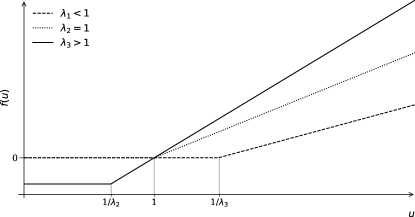
(a) Function $f(u)$ for different values of $\lambda$.

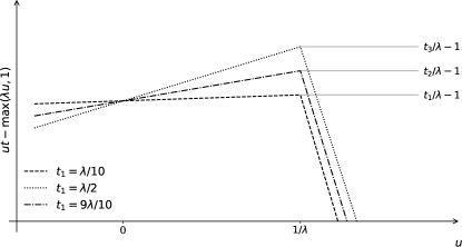
(b) Function $u\mapsto ut-\max(\lambda u,1)$ for values of $t$ between $0$ and $\lambda$.

Consequently the Fenchel conjugate of $f$ is:

$$\forall t\in\left[0,\lambda\right],\quad f^{*}(t)=\max(\lambda,1)+t\lambda-1=\begin{cases}t/\lambda&\mbox{if }\lambda\leq 1,\\ t/\lambda-1+\lambda&\mbox{otherwise. }\end{cases}$$ (26)

Finally, the optimal discriminator $T^{\mathrm{opt}}$ by taking the derivative of $f$ in $\frac{p(\boldsymbol{x})}{\widehat{p}(\boldsymbol{x})}$, we get:

$$T^{\mathrm{opt}}(\boldsymbol{x})=\nabla f\left(\frac{p(\boldsymbol{x})}{\widehat{p}(\boldsymbol{x})}\right)=\begin{cases}\lambda&\mbox{if }\frac{p(\boldsymbol{x})}{\widehat{p}(\boldsymbol{x})}\leq 1/\lambda,\\ 0&\mbox{otherwise}.\end{cases}$$ (27)

Then we can compute the compute the reverse $\mathcal{D}_{\lambda{\scaleto{\mbox{-}\mathrm{PR}}{0.7ex}}}$:

$$\mathcal{D}_{\lambda{\scaleto{\mbox{-}\mathrm{PR}}{0.7ex}}}(\widehat{P}\|P) =\int_{\mathcal{X}}p(\boldsymbol{x})f_{\lambda}\left(\frac{\widehat{p}(\boldsymbol{x})}{p(\boldsymbol{x})}\right)\mathrm{d}\boldsymbol{x}$$ (28)

$$=\int_{\mathcal{X}}\max(\lambda\widehat{p}(\boldsymbol{x}),p(\boldsymbol{x}))-p(\boldsymbol{x})\max(\lambda,1)\,\mathrm{d}\boldsymbol{x}$$ (29)

$$=\lambda\left(\int_{\mathcal{X}}\max(\widehat{p}(\boldsymbol{x}),p(\boldsymbol{x})/\lambda)\partial\boldsymbol{x}-\max(1,1/\lambda)\right)$$ (30)

$$=\lambda\int_{\mathcal{X}}\widehat{p}(\boldsymbol{x})\max(1,\frac{p(\boldsymbol{x})}{\widehat{p}(\boldsymbol{x})}/\lambda)-\widehat{p}(\boldsymbol{x})\max(1,1/\lambda)\,\mathrm{d}\boldsymbol{x}$$ (31)

$$=\lambda\int_{\mathcal{X}}\widehat{p}(\boldsymbol{x})f_{1/\lambda}\left(\frac{p(\boldsymbol{x})}{\widehat{p}(\boldsymbol{x})}\right)\mathrm{d}\boldsymbol{x}$$ (32)

$$=\lambda\mathcal{D}_{\frac{1}{\lambda}{\scaleto{\mbox{-}\mathrm{PR}}{0.7ex}}}(P\|\widehat{P}).$$ (33)

With this results, we can show that :

$$\mathcal{D}_{\mathrm{TV}}(P\|\widehat{P}) =\int_{\mathcal{X}}\left|p(\boldsymbol{x})-\widehat{p}(\boldsymbol{x})\right|\mathrm{d}\boldsymbol{x}$$ (34)

$$=\int_{\mathcal{X}}\max(p(\boldsymbol{x})-\widehat{p}(\boldsymbol{x}),0)+\max(\widehat{p}(\boldsymbol{x})-p(\boldsymbol{x}),0)\mathrm{d}\boldsymbol{x}$$ (35)

Then since $\mathcal{D}_{1{\scaleto{\mbox{-}\mathrm{PR}}{0.7ex}}}(P\|\widehat{P})=\int_{\mathcal{X}}\max(\widehat{p}(\boldsymbol{x}),p(\boldsymbol{x}))-p(\boldsymbol{x})\mathrm{d}\boldsymbol{x}=\int_{\mathcal{X}}p(\boldsymbol{x})\max(\widehat{p}(\boldsymbol{x})\mathrm{d}\boldsymbol{x}$ and $\mathcal{D}_{1{\scaleto{\mbox{-}\mathrm{PR}}{0.7ex}}}(P\|\widehat{P})=\mathcal{D}_{1{\scaleto{\mbox{-}\mathrm{PR}}{0.7ex}}}(\widehat{P}\|P)$, we have:

$$\mathcal{D}_{\mathrm{TV}}(P\|\widehat{P}) =\mathcal{D}_{1{\scaleto{\mbox{-}\mathrm{PR}}{0.7ex}}}(P\|\widehat{P})+\mathcal{D}_{1{\scaleto{\mbox{-}\mathrm{PR}}{0.7ex}}}(\widehat{P}\|\P)$$ (36)

$$=2\mathcal{D}_{1{\scaleto{\mbox{-}\mathrm{PR}}{0.7ex}}}(P\|\widehat{P}).$$ (37)

A.3 Proof of Theorem 5.2

From now on, assume the support of $P$ and $\widehat{P}$ coincide. For any $T:\mathcal{X}\rightarrow\mathbb{R}$,

$$\mathcal{D}^{\mathrm{dual}}_{f,T}(P\|\widehat{P}) =\mathbb{E}_{x\sim P}\left[d\left(x\right)\right]-\mathbb{E}_{x\sim Q}\left[f^{*}\left(d\left(x\right)\right)\right]$$

$$=\mathbb{E}_{x\sim Q}\left[\frac{p(\boldsymbol{x})}{\widehat{p}(\boldsymbol{x})}d\left(x\right)-f^{*}\left(d\left(x\right)\right)\right]$$

Let $T^{\mathrm{opt}}\in\arg\sup\mathcal{D}_{f,T}^{\mathrm{dual}}(P\|\widehat{P})$. For any $T:\mathcal{X}\rightarrow\mathbb{R}$

$$\mathcal{D}_{f}(P\|\widehat{P})-D_{f,T}^{\mathrm{dual}}(P\|\widehat{P}) =\mathcal{D}_{f,T^{\mathrm{opt}}}^{\mathrm{dual}}(P\|\widehat{P})-\mathcal{D}_{f,T}^{\mathrm{dual}}(P\|\widehat{P})$$

$$=\mathbb{E}_{\widehat{P}}\left[\frac{p(\boldsymbol{x})}{\widehat{p}(\boldsymbol{x})}\left(T^{\mathrm{opt}}(\boldsymbol{x})-T(\boldsymbol{x})\right)-f^{*}\left(T^{\mathrm{opt}}(\boldsymbol{x})\right)+f^{*}\left(T(\boldsymbol{x})\right)\right]$$

It is known that for all $x\in\mathcal{X}$ we have $\nabla f^{*}(T^{\mathrm{opt}}(\boldsymbol{x}))=\frac{p(\boldsymbol{x})}{\widehat{p}(\boldsymbol{x})}$:

$$\mathcal{D}_{f}(P\|\widehat{P})-\mathcal{D}_{f,T}^{\mathrm{dual}}(P\|\widehat{P}) =\mathbb{E}_{\widehat{P}}\left[\nabla f^{*}(T^{\mathrm{opt}}(\boldsymbol{x}))\left(T^{\mathrm{opt}}(\boldsymbol{x})-T(\boldsymbol{x})\right)-f^{*}\left(T^{\mathrm{opt}}(\boldsymbol{x})\right)+f^{*}\left(T(\boldsymbol{x})\right)\right]$$

Recall that for any continuously differentiable strictly convex function$f$, the Bregman divergence of $f$ is $\mathrm{Breg}_{f}\left(a,b\right)=f(a)-f(b)-\left\langle\nabla f(b),a-b\right\rangle$. So we have

$$\mathcal{D}_{f}(P\|\widehat{P})-\mathcal{D}_{f,T}^{\mathrm{dual}}(P\|\widehat{P}) =\mathbb{E}_{\widehat{P}}\left[\mathrm{Breg}_{f^{*}}\left(T(\boldsymbol{x}),T^{\mathrm{opt}}(\boldsymbol{x})\right)\right]$$

Let us now use the following property: $\mathrm{Breg}_{f}\left(a,b\right)=\mathrm{Breg}_{f^{*}}\left(a^{*},b^{*}\right)$ where $a^{*}=\nabla f(a)$ and $b^{*}=\nabla f(b)$.

$$\mathcal{D}_{f}(P\|\widehat{P})-\mathcal{D}_{f,T}^{\mathrm{dual}}(P\|\widehat{P}) =\mathbb{E}_{\widehat{P}}\left[\mathrm{Breg}_{f}\left(\nabla f^{*}(T(\boldsymbol{x})),\nabla f^{*}(T^{\mathrm{opt}}(\boldsymbol{x}))\right)\right]$$

$$=\mathbb{E}_{\widehat{P}}\left[\mathrm{Breg}_{f}\left(\nabla f^{*}(T(\boldsymbol{x})),\frac{p(\boldsymbol{x})}{\widehat{p}(\boldsymbol{x})}\right)\right]$$

Let us define $r\left(\boldsymbol{x}\right)=\nabla f^{*}T(\boldsymbol{x})$ as our estimator of $p(\boldsymbol{x})/\widehat{p}(\boldsymbol{x})$. So finally, we have

$$\mathcal{D}_{f}(P\|\widehat{P})-\mathcal{D}_{f,T}^{\mathrm{dual}}(P\|\widehat{P}) =\mathbb{E}_{\widehat{P}}\left[\mathrm{Breg}_{f}\left(r(\boldsymbol{x}),\frac{p(\boldsymbol{x})}{\widehat{p}(\boldsymbol{x})}\right)\right]$$

A.4 Proof of Theorem 5.3

Now assume that $f$ is $\mu$-strongly convex, then $\mathrm{Breg}_{f}(a,b)\geq\frac{\mu}{2}\left\|a-b\right\|^{2}$ If $\mathbb{E}_{\widehat{P}}\left[\mathrm{Breg}_{f}\left(r(\boldsymbol{x}),\frac{p(\boldsymbol{x})}{\widehat{p}(\boldsymbol{x})}\right)\right]\leq\epsilon$ and if $f$ is $\mu$-strongly convex, then

$$\mathbb{E}_{\widehat{P}}\left[\left(r(\boldsymbol{x})-\frac{p(\boldsymbol{x})}{\widehat{p}(\boldsymbol{x})}\right)^{2}\right]\leq\frac{2\epsilon}{\mu}.$$ (38)

Consider an arbitrary f-divergence $\mathcal{D}_{g}(P\|\widehat{P})=\int g\left(\frac{dP}{\mathrm{d}\widehat{P}}\right)\mathrm{d}\widehat{P}$. Define $\mathcal{D}_{g,T}^{\mathrm{primal}}(P\|\widehat{P})=\int g\left(r(\boldsymbol{x})\right)\mathrm{d}\widehat{P}$. Then,

$$\left|\mathcal{D}_{g}(P\|\widehat{P})-\mathcal{D}_{g,T}^{\mathrm{primal}}(P\|\widehat{P})\right| =\left|\mathbb{E}_{\widehat{P}}\left[g\left(\frac{p(\boldsymbol{x})}{\widehat{p}(\boldsymbol{x})}\right)-g\left(r(\boldsymbol{x})\right)\right]\right|$$

$$\leq\mathbb{E}_{\widehat{P}}\left[\left|g\left(\frac{p(\boldsymbol{x})}{\widehat{p}(\boldsymbol{x})}\right)-g\left(r(\boldsymbol{x})\right)\right|\right]$$

$$\stackrel{{\scriptstyle(a)}}{{\leq}}\mathbb{E}_{\widehat{P}}\left[\sigma\left|e(x)\right|\right]$$

$$=\sigma\mathbb{E}_{\widehat{P}}\left[\left|e(x)\right|\right]$$

$$\stackrel{{\scriptstyle(b)}}{{\leq}}\sigma\sqrt{\mathbb{E}_{\widehat{P}}\left[e(x)^{2}\right]}$$

$$\stackrel{{\scriptstyle(c)}}{{\leq}}\sigma\sqrt{\frac{2\epsilon}{\mu}},$$

where $(a)$ follows from the $\sigma$-Lipschitz assumption on $g$, $(b)$ follows from Jensen’s inequality and finally, $(c)$ follows from equation (38).

A.5 Proof of Theorem 10

Let $c:\mathbb{R}^{+}\mapsto\mathbb{R}$ be a $\mathcal{C}^{2}$ function and take $u_{\min}$ and $u_{\max}$. The goal is to express $f(u)$ for all $u\in[u_{\min},u_{\max}]$ as a weighted average of $f^{\mathrm{PR}}_{\lambda}$:

$$\forall u\in\mathbb{R}_{*}^{+},\int_{1/u_{\max}}^{1/u_{\min}}c^{\prime\prime}(\lambda)f^{\mathrm{PR}}_{\lambda}(u)\mathrm{d}\lambda=\int_{1/u_{\max}}^{1/u_{\min}}c^{\prime\prime}(\lambda)\left[\max(\lambda u,1)-\max\left(\lambda,1\right)\right]\mathrm{d}\lambda$$ (39)

First, let us assume that $u_{\min}\leq 1$ and $u_{\max}\geq 1$, then the terms can be decomposed and the integral split to evaluate the $\max$:

$$\int_{1/u_{\max}}^{1/u_{\min}}c^{\prime\prime}(\lambda)f^{\mathrm{PR}}_{\lambda}(u)\mathrm{d}\lambda =\int_{1/u_{\max}}^{1/u_{\min}}c^{\prime\prime}(\lambda)\max(\lambda u,1)\mathrm{d}\lambda-\int_{1/u_{\max}}^{1/u_{\min}}c^{\prime\prime}(\lambda)\max\left(\lambda,1\right)\mathrm{d}\lambda$$ (40)

$$=\begin{multlined}\int_{1/u_{\max}}^{1/u}c^{\prime\prime}(\lambda)\max(\lambda u,1)\mathrm{d}\lambda+\int_{1/u}^{1/u_{\min}}c^{\prime\prime}(\lambda)\max(\lambda u,1)\mathrm{d}\lambda\\ -\int_{1/u_{\max}}^{1}c^{\prime\prime}(\lambda)\max\left(\lambda,1\right)\mathrm{d}\lambda-\int_{1}^{1/u_{\min}}c^{\prime\prime}(\lambda)\max\left(\lambda,1\right)\mathrm{d}\lambda\end{multlined}\int_{1/u_{\max}}^{1/u}c^{\prime\prime}(\lambda)\max(\lambda u,1)\mathrm{d}\lambda+\int_{1/u}^{1/u_{\min}}c^{\prime\prime}(\lambda)\max(\lambda u,1)\mathrm{d}\lambda\\ -\int_{1/u_{\max}}^{1}c^{\prime\prime}(\lambda)\max\left(\lambda,1\right)\mathrm{d}\lambda-\int_{1}^{1/u_{\min}}c^{\prime\prime}(\lambda)\max\left(\lambda,1\right)\mathrm{d}\lambda$$ (43)

$$=\int_{1/u_{\max}}^{1/u}c^{\prime\prime}(\lambda)\mathrm{d}\lambda+\int_{1/u}^{1/u_{\min}}c^{\prime\prime}(\lambda)\lambda u\mathrm{d}\lambda-\int_{1/u_{\max}}^{1}c^{\prime\prime}(\lambda)\mathrm{d}\lambda-\int_{1}^{1/u_{\min}}c^{\prime\prime}(\lambda)\lambda\mathrm{d}\lambda.$$ (44)

By integrating by parts, we have: $\int_{1/u_{\max}}^{1/u_{\min}}c^{\prime\prime}(\lambda)\lambda\mathrm{d}\lambda=\left[c^{\prime}(\lambda)\lambda\right]_{1/u_{\max}}^{1/u_{\min}}-\int_{1/u_{\max}}^{1/u_{\min}}c^{\prime}(\lambda)\mathrm{d}\lambda$ so it satisfies:

$$\int_{1/u_{\max}}^{1/u_{\min}}c^{\prime\prime}(\lambda)f^{\mathrm{PR}}_{\lambda}(u)\mathrm{d}\lambda =\begin{multlined}\int_{1/u_{\max}}^{1/u}c^{\prime\prime}(\lambda)\mathrm{d}\lambda+u\left[c^{\prime}(\lambda)\lambda\right]_{1/u}^{1/u_{\min}}-u\int_{1/u}^{1/u_{\min}}c^{\prime}(\lambda)\mathrm{d}\lambda\\ -\int_{1/u_{\max}}^{1}c^{\prime\prime}(\lambda)\mathrm{d}\lambda-\left[c^{\prime}(\lambda)\lambda\right]_{1}^{1/u_{\min}}+\int_{1}^{1/u_{\min}}c^{\prime}(\lambda)\mathrm{d}\lambda\end{multlined}\int_{1/u_{\max}}^{1/u}c^{\prime\prime}(\lambda)\mathrm{d}\lambda+u\left[c^{\prime}(\lambda)\lambda\right]_{1/u}^{1/u_{\min}}-u\int_{1/u}^{1/u_{\min}}c^{\prime}(\lambda)\mathrm{d}\lambda\\ -\int_{1/u_{\max}}^{1}c^{\prime\prime}(\lambda)\mathrm{d}\lambda-\left[c^{\prime}(\lambda)\lambda\right]_{1}^{1/u_{\min}}+\int_{1}^{1/u_{\min}}c^{\prime}(\lambda)\mathrm{d}\lambda$$ (47)

$$=\begin{multlined}\left[c^{\prime}(\lambda)\right]_{1/u_{\max}}^{1/u}+u\left[c^{\prime}(\lambda)\lambda\right]_{1/u}^{1/u_{\min}}-u\left[c(\lambda)\right]_{1/u}^{1/u_{\min}}\\ -\left[c^{\prime}(\lambda)\right]_{1/u_{\max}}^{1}-\left[c^{\prime}(\lambda)\lambda\right]_{1}^{1/u_{\min}}+\left[c(\lambda)\right]_{1}^{1/u_{\min}}\end{multlined}\left[c^{\prime}(\lambda)\right]_{1/u_{\max}}^{1/u}+u\left[c^{\prime}(\lambda)\lambda\right]_{1/u}^{1/u_{\min}}-u\left[c(\lambda)\right]_{1/u}^{1/u_{\min}}\\ -\left[c^{\prime}(\lambda)\right]_{1/u_{\max}}^{1}-\left[c^{\prime}(\lambda)\lambda\right]_{1}^{1/u_{\min}}+\left[c(\lambda)\right]_{1}^{1/u_{\min}}$$ (50)

$$=\begin{multlined}c^{\prime}\left(\frac{1}{u}\right)-c^{\prime}(0)+uc^{\prime}\left(\frac{1}{u_{\min}}\right)-uc^{\prime}\left(\frac{1}{u}\right)\frac{1}{u}-uc\left(\frac{1}{u_{\min}}\right)+uc\left(\frac{1}{u}\right)-c^{\prime}(1)\\ +c^{\prime}(0)-c^{\prime}\left(\frac{1}{u_{\min}}\right)\frac{1}{u_{\min}}+c^{\prime}(1)\times 1+c\left(\frac{1}{u_{\min}}\right)-c(1)\end{multlined}c^{\prime}\left(\frac{1}{u}\right)-c^{\prime}(0)+uc^{\prime}\left(\frac{1}{u_{\min}}\right)-uc^{\prime}\left(\frac{1}{u}\right)\frac{1}{u}-uc\left(\frac{1}{u_{\min}}\right)+uc\left(\frac{1}{u}\right)-c^{\prime}(1)\\ +c^{\prime}(0)-c^{\prime}\left(\frac{1}{u_{\min}}\right)\frac{1}{u_{\min}}+c^{\prime}(1)\times 1+c\left(\frac{1}{u_{\min}}\right)-c(1)$$ (53)

$$=\left[c^{\prime}\left(\frac{1}{u_{\min}}\right)\frac{1}{u_{\min}}-c\left(\frac{1}{u_{\min}}\right)\right]\left(u-1\right)+uc\left(\frac{1}{u}\right)-c(1).$$ (54)

We would like $\int_{1/u_{\max}}^{1/u_{\min}}c^{\prime\prime}(\lambda)f^{\mathrm{PR}}_{\lambda}(u)\mathrm{d}\lambda$ to be equal to $f$ between $u_{\min}$ and $u_{\max}$. But since two $f$-divergences generated by $f$ and $g$ are equals if there is a $c\in\mathbb{R}$ such that $f(u)=g(u)+c(u-1)$, the Divergence generated by $\int_{1/u_{\max}}^{1/u_{\min}}c^{\prime\prime}(\lambda)f^{\mathrm{PR}}_{\lambda}(u)\mathrm{d}\lambda$ is equal to the divergence generated by $uc\left(\frac{1}{u}\right)-c(1)$. Therefore, we require $c$ to satisfy:

$$\forall u\in[u_{\min},u_{\max}],\quad f(u)=uc\left(\frac{1}{u}\right)-c(1).$$

By differentiating with respect to $u$, we have:

$$f^{\prime}(u)=\lim_{\lambda\rightarrow\infty}\left[c^{\prime}(\lambda)\lambda-c(\lambda)\right]+c\left(\frac{1}{u}\right)-\frac{1}{u}c^{\prime}\left(\frac{1}{u}\right).$$ (55)

And finally:

$$f^{\prime\prime}(u) =-\frac{1}{u^{2}}c\left(\frac{1}{u}\right)+\frac{1}{u^{2}}c^{\prime}\left(\frac{1}{u}\right)+\frac{1}{u^{3}}c^{\prime\prime}\left(\frac{1}{u}\right)$$ (56)

$$=\frac{1}{u^{3}}c^{\prime\prime}\left(\frac{1}{u}\right).$$ (57)

Consequently, with $\lambda=1/u$, we have that:

$$c^{\prime\prime}(\lambda)=\frac{1}{\lambda^{3}}f^{\prime\prime}\left(\frac{1}{\lambda}\right).$$ (58)

With such a results, with $m=\min_{\mathcal{X}}(\frac{\widehat{p}(\boldsymbol{x})}{p(\boldsymbol{x})})$ and $M=\max_{\mathcal{X}}(\frac{\widehat{p}(\boldsymbol{x})}{p(\boldsymbol{x})})$, we can write any $f$-divergence as:

$$\mathcal{D}_{f}(P\|\widehat{P}) =\int_{\mathcal{X}}\widehat{p}(\boldsymbol{x})f\left(\frac{p(\boldsymbol{x})}{\widehat{p}(\boldsymbol{x})}\right)\mathrm{d}\boldsymbol{x}$$

$$=\int_{\mathcal{X}}\widehat{p}(\boldsymbol{x})\int_{m}^{M}\frac{1}{\lambda^{3}}f^{\prime\prime}\left(\frac{1}{\lambda}\right)f^{\mathrm{PR}}_{\lambda}\left(\frac{p(\boldsymbol{x})}{\widehat{p}(\boldsymbol{x})}\right)\mathrm{d}\lambda\mathrm{d}\boldsymbol{x}$$

$$=\int_{m}^{M}\int_{\mathcal{X}}\frac{1}{\lambda^{3}}f^{\prime\prime}\left(\frac{1}{\lambda}\right)\widehat{p}(\boldsymbol{x})f^{\mathrm{PR}}_{\lambda}\left(\frac{p(\boldsymbol{x})}{\widehat{p}(\boldsymbol{x})}\right)\mathrm{d}\lambda\mathrm{d}\boldsymbol{x}$$

$$=\int_{m}^{M}\frac{1}{\lambda^{3}}f^{\prime\prime}\left(\frac{1}{\lambda}\right)\left[\int_{\mathcal{X}}\widehat{p}(\boldsymbol{x})f^{\mathrm{PR}}_{\lambda}\left(\frac{p(\boldsymbol{x})}{\widehat{p}(\boldsymbol{x})}\right)\mathrm{d}\boldsymbol{x}\right]\mathrm{d}\lambda$$

$$=\int_{m}^{M}\frac{1}{\lambda^{3}}f^{\prime\prime}\left(\frac{1}{\lambda}\right)\mathcal{D}_{\lambda{\scaleto{\mbox{-}\mathrm{PR}}{0.7ex}}}(P\|\widehat{P})\mathrm{d}\lambda$$

A.6 Proof of Corollary 4.5

In particular for the $\mathcal{D}_{\mathrm{KL}}$, $f(u)=u\log u$, therefore $f^{\prime\prime}(u)=1/u$ which gives:

$$\mathcal{D}_{\mathrm{KL}}(P\|\widehat{P})=\int_{m}^{M}\frac{1}{\lambda^{2}}\mathcal{D}_{\lambda{\scaleto{\mbox{-}\mathrm{PR}}{0.7ex}}}(P\|\widehat{P})\mathrm{d}\lambda.$$ (59)

And for the $\mathcal{D}_{\mathrm{rKL}}$ we can either use Equation 58 with $f(u)-\log u$ or use the fact that $\mathcal{D}_{\lambda{\scaleto{\mbox{-}\mathrm{PR}}{0.7ex}}}(P\|\widehat{P})=\lambda\mathcal{D}_{1/\lambda{\scaleto{\mbox{-}\mathrm{PR}}{0.7ex}}}(\widehat{P}\|P)$:

$$\mathcal{D}_{\mathrm{rKL}}(P\|\widehat{P})=\int_{m}^{M}\frac{1}{\lambda}\mathcal{D}_{\lambda{\scaleto{\mbox{-}\mathrm{PR}}{0.7ex}}}(P\|\widehat{P})\mathrm{d}\lambda.$$ (60)

A.7 Proof of Proposition 6.1

The AUC can be computed by integrating with respect to an angle $\theta$ on the quadrant:

$$\mathrm{AUC}=\int_{0}^{\pi/2}r^{2}(\theta)\mathrm{d}\theta.$$ (61)

Therefore with $\lambda=\tan\theta$, we have $r(\theta)=\alpha_{\tan(\theta)}(P\|\widehat{P})/\cos\theta$. Thus:

$$\mathrm{AUC} =\int_{0}^{\pi/2}\frac{\alpha_{\tan(\theta)}(P\|\widehat{P})^{2}}{\cos^{2}\theta}\mathrm{d}\theta$$ (62)

$$=\int_{0}^{+\infty}\alpha_{\lambda}(P\|\widehat{P})^{2}\cos^{2}\theta\mathrm{d}\lambda\quad\mbox{with }\quad\frac{\mathrm{d}\theta}{\cos^{2}\theta}=\partial\lambda.$$ (63)

Figure A.8: Illustration of the change of variable to compute the AUC. Instead of parametrising the frontier $\partial\mathrm{PRD}(P,\widehat{P})$ with $\lambda\in\mathbb{R}\cup\left\{\infty\right\}$, we take $\theta\in\left[0,\frac{\pi}{2}\right]$ with $\lambda=\tan\theta$.

Appendix B Experiments

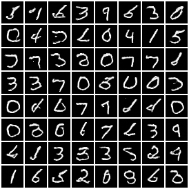
(a) $\lambda=\frac{1}{5}$

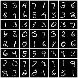
(b) $\lambda=1$

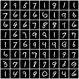
(c) $\lambda=5$

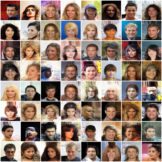
(d) $\lambda=\frac{1}{5}$

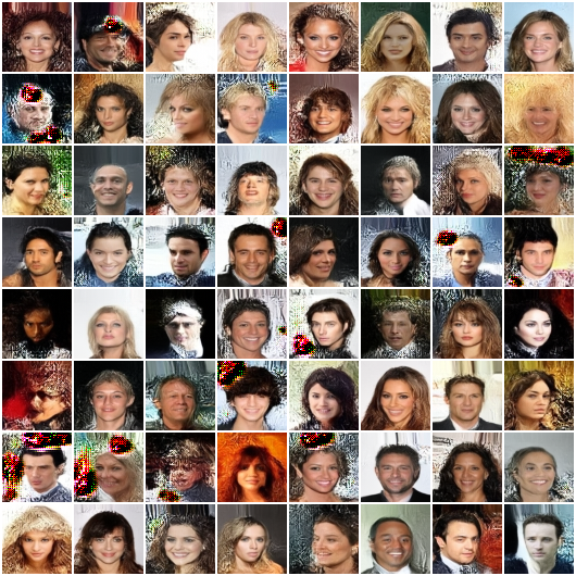
(e) $\lambda=1$

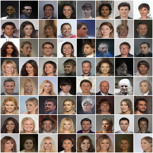
(f) $\lambda=5$

Figure B.9: Large batch of samples for different Glow models trained on MNIST ((a), (b) and (c)) and CelebaA ((d), (e) and (f)). Models have been trained to minimise $\mathcal{D}_{\lambda{\scaleto{\mbox{-}\mathrm{PR}}{0.7ex}}}$ with different $\lambda$ given in caption. The lower $\lambda$ is, the greater the model will value the recall, while precision is highly considered for high values of $\lambda$.

The details of the experiments are described in Table LABEL:app:xptab

Dataset	Model	#Parameters $F$	#Parameters $D$
8 Gaussians	RealNVP	$540$k	$659$k
MNIST	Glow	$85$M	$1.7$M
CelabA	Glow	$188$M	$13.2$M

Table 2: Details of the models for the different experiments.

References

- Arjovsky et al. (2017) Arjovsky, M., Chintala, S., and Bottou, L. Wasserstein GAN. In Proceedings of the 34th International Conference on Machine Learning, Sydney, Australia,, December 2017. URL http://arxiv.org/abs/1701.07875. arXiv: 1701.07875.
- Behrmann et al. (2019) Behrmann, J., Grathwohl, W., Chen, R. T. Q., Duvenaud, D., and Jacobsen, J.-H. Invertible Residual Networks. In Proceedings of the 36 th International Conference on Machine Learning, Long Beach, California, PMLR 97, 2019, May 2019. arXiv: 1811.00995.
- Chen et al. (2020) Chen, R. T. Q., Behrmann, J., Duvenaud, D., and Jacobsen, J.-H. Residual Flows for Invertible Generative Modeling. In 33rd Conference on Neural Information Processing Systems (NeurIPS 2019), Vancouver, Canada., July 2020. arXiv: 1906.02735.
- Djolonga et al. (2020) Djolonga, J., Lucic, M., Cuturi, M., Bachem, O., Bousquet, O., and Gelly, S. Precision-Recall Curves Using Information Divergence Frontiers, June 2020. URL http://arxiv.org/abs/1905.10768. arXiv:1905.10768 [cs, stat].
- Grover et al. (2018) Grover, A., Dhar, M., and Ermon, S. Flow-GAN: Combining Maximum Likelihood and Adversarial Learning in Generative Models, January 2018. URL http://arxiv.org/abs/1705.08868. arXiv:1705.08868 [cs, stat].
- Heusel et al. (2017) Heusel, M., Ramsauer, H., Unterthiner, T., Nessler, B., and Hochreiter, S. GANs Trained by a Two Time-Scale Update Rule Converge to a Local Nash Equilibrium. In Advances in Neural Information Processing Systems, volume 30. Curran Associates, Inc., 2017. URL https://proceedings.neurips.cc/paper/2017/hash/8a1d694707eb0fefe65871369074926d-Abstract.html.
- Issenhuth et al. (2022) Issenhuth, T., Tanielian, U., Picard, D., and Mary, J. Latent reweighting, an almost free improvement for GANs. In 2022 IEEE/CVF Winter Conference on Applications of Computer Vision (WACV), pp. 3574–3583, Waikoloa, HI, USA, January 2022. IEEE. ISBN 978-1-66540-915-5. doi: 10.1109/WACV51458.2022.00363. URL https://ieeexplore.ieee.org/document/9706934/.
- Kingma & Dhariwal (2018) Kingma, D. P. and Dhariwal, P. Glow: Generative Flow with Invertible 1x1 Convolutions. In 32nd Conference on Neural Information Processing Systems (NeurIPS 2018), Montréal, Canada., volume 31, 2018.
- Kobyzev et al. (2020) Kobyzev, I., Prince, S. J. D., and Brubaker, M. A. Normalizing Flows: An Introduction and Review of Current Methods. IEEE Transactions on Pattern Analysis and Machine Intelligence, pp. 1–1, 2020. ISSN 0162-8828, 2160-9292, 1939-3539. doi: 10.1109/TPAMI.2020.2992934. URL http://arxiv.org/abs/1908.09257. arXiv: 1908.09257.
- Kynkäänniemi et al. (2019) Kynkäänniemi, T., Karras, T., Laine, S., Lehtinen, J., and Aila, T. Improved Precision and Recall Metric for Assessing Generative Models. In 33rd Conference on Neural Information Processing Systems (NeurIPS 2019), Vancouver, Canada., October 2019. arXiv: 1904.06991.
- Liu et al. (2015) Liu, Z., Luo, P., Wang, X., and Tang, X. Deep Learning Face Attributes in the Wild, September 2015. URL http://arxiv.org/abs/1411.7766. arXiv:1411.7766 [cs].
- Midgley et al. (2022a) Midgley, L. I., Stimper, V., Simm, G. N. C., and Hernández-Lobato, J. M. Bootstrap Your Flow, March 2022a. URL http://arxiv.org/abs/2111.11510. arXiv:2111.11510 [cs, stat].
- Midgley et al. (2022b) Midgley, L. I., Stimper, V., Simm, G. N. C., Schölkopf, B., and Hernández-Lobato, J. M. Flow Annealed Importance Sampling Bootstrap, November 2022b. URL http://arxiv.org/abs/2208.01893. arXiv:2208.01893 [cs, q-bio, stat].
- Minka (2005) Minka, T. Divergence measures and message passing. pp. 17, 2005.
- Nguyen et al. (2009) Nguyen, X., Wainwright, M. J., and Jordan, M. I. On surrogate loss functions and $f$-divergences. The Annals of Statistics, 37(2), April 2009. ISSN 0090-5364. doi: 10.1214/08-AOS595. URL http://arxiv.org/abs/math/0510521. arXiv:math/0510521.
- Nowozin et al. (2016) Nowozin, S., Cseke, B., and Tomioka, R. f-GAN: Training Generative Neural Samplers using Variational Divergence Minimization, June 2016. URL http://arxiv.org/abs/1606.00709. arXiv:1606.00709 [cs, stat].
- Rezende & Mohamed (2016) Rezende, D. J. and Mohamed, S. Variational Inference with Normalizing Flows. In arXiv:1505.05770 [cs, stat], June 2016.
- Sajjadi et al. (2018) Sajjadi, M. S. M., Bachem, O., Lucic, M., Bousquet, O., and Gelly, S. Assessing Generative Models via Precision and Recall. In 32nd Conference on Neural Information Processing Systems (NeurIPS 2018), Montréal, Canada, October 2018. URL http://arxiv.org/abs/1806.00035. arXiv: 1806.00035.
- Salimans et al. (2016) Salimans, T., Goodfellow, I., Zaremba, W., Cheung, V., Radford, A., and Chen, X. Improved Techniques for Training GANs, June 2016. URL http://arxiv.org/abs/1606.03498. arXiv:1606.03498 [cs].
- Simon et al. (2019) Simon, L., Webster, R., and Rabin, J. Revisiting precision recall definition for generative modeling. In Proceedings of the 36th International Conference on Machine Learning, pp. 5799–5808. PMLR, May 2019. URL https://proceedings.mlr.press/v97/simon19a.html. ISSN: 2640-3498.
- Stimper et al. (2022) Stimper, V., Schölkopf, B., and Hernández-Lobato, J. M. Resampling Base Distributions of Normalizing Flows. arXiv:2110.15828 [cs, stat], February 2022. URL http://arxiv.org/abs/2110.15828. arXiv: 2110.15828.
- Tanielian et al. (2020) Tanielian, U., Issenhuth, T., Dohmatob, E., and Mary, J. Learning disconnected manifolds: a no GANs land. In Proceedings of the 37 th International Conference on Machine Learning, Vienna, Austria, PMLR 119, 2020, December 2020. arXiv: 2006.04596.
- Yann LeCun et al. (2010) Yann LeCun, Corinna Cortes, and Burges, C. MNIST handwritten digit database. ATT Labs, 2, 2010. URL http://yann.lecun.com/exdb/mnist.