Open-VCLIP: Transforming CLIP to an Open-vocabulary Video Model
via Interpolated Weight Optimization

Abstract

Contrastive Language-Image Pretraining (CLIP) has demonstrated impressive zero-shot learning abilities for image understanding, yet limited effort has been made to investigate CLIP for zero-shot video recognition. We introduce Open-VCLIP, a simple yet effective approach that transforms CLIP into a strong zero-shot video classifier that can recognize unseen actions and events at test time. Our framework extends CLIP with minimal modifications to model spatial-temporal relationships in videos, making it a specialized video classifier, while striving for generalization. We formally show that training an Open-VCLIP is equivalent to continual learning with zero historical data. To address this problem, we propose Interpolated Weight Optimization, which utilizes the benefit of weight interpolation in both training and test time. We evaluate our method on three popular and challenging action recognition datasets following various zero-shot evaluation protocols and we demonstrate our approach outperforms state-of-the-art methods by clear margins. In particular, we achieve 87.9%, 58.3%, 81.1% zero-shot accuracy on UCF, HMDB and Kinetics-600 respectively, outperforming state-of-the-art methods by 8.3%, 7.8% and 12.2%. Code is released at https://github.com/wengzejia1/Open-VCLIP.

1 Introduction

Zero-shot learning is a challenging problem that requires deep neural networks to recognize novel unseen classes during testing without having seen them during training. The generalization ability of classifying new classes without the need for manual annotations makes it particularly useful in real-world applications. While extensive studies have been conducted on zero-shot learning (Zellers & Choi, 2017; Brattoli et al., 2020; Xu et al., 2017), CLIP (Radford et al., 2021) recently demonstrates surprising zero-shot abilities in a variety of tasks, such as image segmentation (Wang et al., 2022; Ghiasi et al., 2021, 2022), image editing (Zheng et al., 2022; Crowson et al., 2022), by pretraining on web-scale image and text pairs in a contrastive manner.

Figure 1: While CLIP has shown impressive results for zero-shot image recognition, it cannot effectively recognize novel actions in videos. This paper aims to transform CLIP to a strong zero-shot video classifier with minimal modifications.

While significant zero-shot results are achieved in the image domain, limited effort has been made to explore CLIP for zero-shot video action recognition. Extending CLIP, designed for image tasks, to the video domain, is extremely challenging, particularly in the zero-shot setting. On one hand, to better recognize actions and events in videos, the rich temporal dynamics encoded in videos are expected to be carefully captured. Although one could treat videos as a bag of frames and perform temporal pooling over frame-based predictions (Wang et al., 2021), it is found that fine-tuning pretrained models like CLIP with specialized temporal modeling components on top of off-the-shelf image models produces better results (Ni et al., 2022). However, the improved results come at the cost of reduced generalization as optimizing specialized parameters will inevitably requires fine-tuning the pretrained CLIP model. The derived model then tends to overfit to the video dataset used for fine-tuning, which are substantially smaller than the image-text dataset used to train CLIP. As a result, the zero-shot ability of CLIP diminishes over the course of fine-tuning.

It is worth noting that the start point of the fine-tuning process is CLIP, an image classifier with strong zero-shot abilities, while the end point is a specialized model for video understanding. This motivates us to seek a middle ground between generalization and specialization—adapting a pretrained CLIP model to the video domain, and the resulting model is expected to not only recognize known actions and events seen during training but also enjoy the zero-shot learning abilities as CLIP for novel video categories. Interestingly, we discover from a theoretical perspective that this problem is essentially a continual learning problem, which aims to adapt a pretrained model to new tasks with less forgetting on previous knowledge. Traditional continual learning typically seeks decent performance on all seen tasks with access to historical data (Hu et al., 2021; Balaji et al., 2020; Shin et al., 2017). However, this is particularly challenging for adapting CLIP as raw data used for training are private. Furthermore, our goal is slightly beyond continual learning: we hope to adapt CLIP to be a strong zero-shot video learner that generalizes well to unknown video actions and events, rather than exactly preserving its knowledge for image tasks, which again is difficult without access to the training data of CLIP.

With this in mind, we explore the problem of constructing an open-vocabulary video CLIP by simply leveraging the pretrained weights that are publicly available. More specifically, we build upon CLIP with minimal modifications so as to derive a video action recognition model that can not only capture temporal information among different frames but also generalizes well to unseen actions and events during testing. To optimize the continual learning-based training formulation, we propose a novel method called Interpolated Weight Optimization which regularizes the fine-tuning process of the CLIP model by adding a link between the original CLIP model and the current model. This prevents the derived model from drifting away from CLIP, which we argue is beneficial for generalization. Furthermore, in addition to training, we also link derived optima along the optimization trajectory at test time for improved generalization.

We conduct extensive experiments to evaluate the performance of Open-VCLIP. In particular, we use Kinetics-400 as a proxy dataset to extend CLIP to the video domain and evaluate its zero-shot performance on UCF-101, HMDB-51 and Kinetics-600 with various evaluation protocols. Open-VCLIP achieves state-of-the-art zero-shot video action recognition performance, offering 87.9%, 58.3%, 81.1% zero-shot accuracy on UCF, HMDB and Kinetics-600 respectively, which are 8.3%, 7.8% and 12.2% better compared to alternative methods. Furthermore, Open-VCLIP also achieves the best trade-off between close-set and zero-shot performance across all the benchmarks.

2 Related Work

Zero-shot Video Action Recognition. Zero-shot video action recognition requires models to recognize new actions that are not seen during training, which is useful in real-world applications where data and their corresponding labels are difficult to collect. Early work focuses more on how to represent actions properly. For example, manually-crafted attributes (Liu et al., 2011; Zellers & Choi, 2017), object features (Jain et al., 2015; Gao et al., 2019) are used to represent actions. Researchers also use word embeddings of actions (Brattoli et al., 2020; Xu et al., 2017) as textual semantic representations. Recently, pretraining with large-scale vision-text data is gaining attention, as it achieves impressive results for zero-shot image classification (Radford et al., 2021; Jia et al., 2021). There is also a plethora of work using knowledge learned in large-scale pretrained vision-language models to down-stream tasks in a zero-shot manner (Wang et al., 2022; Ghiasi et al., 2021, 2022). While extensive studies have been conducted for zero-shot image understanding, zero-shot video classification remains less explored. ActionCLIP (Wang et al., 2021) and XCLIP experiment with zero-shot setting for action recognition (Ni et al., 2022), but use the same strategy as in images for zero-shot learning and ignore the forgetting problem when adapting the CLIP model. In contrast, our goal is to explicitly build a strong open-vocabulary zero-shot video classifier by regularizing the fine-tuning process.

Continual Learning. Continual learning aims at training a model on multiple sequential tasks without catastrophically forgetting knowledge from previous tasks. Existing approaches can be divided into three categories: memory-based, expansion based and regularization-based methods. Memory-based methods typically utilize a replay buffer to store past examples or related information such as gradients (Farajtabar et al., 2020). In addition, memory replay is effective for continual learning (Hu et al., 2021; Balaji et al., 2020), however, in our case, it is not feasible to directly use these approaches as historical data are not available. Expansion-based methods (Rusu et al., 2016) expand the network over time in order to maintain past performance. Closest to our approach, perhaps are regularization-based methods (Yin et al., 2020) such as EWC (Kirkpatrick et al., 2017), which add a regularization term to the optimization that constrains new model weights to be close to the original ones. But still historical data need to be used to calculate the Fisher information matrix for approaches like (Kirkpatrick et al., 2017). Our approach differs from standard continual learning in that we wish to transfer the knowledge, i.e. the ability to perform zero-shot learning, from a previous image task to video tasks without access to historical data at all.

3 Preliminary: Video Action Recognition Using CLIP

Video action recognition is a fundamental yet challenging task that often requires intensive model training on large-scale datasets. Inspired by the success of contrastive language-image pretraining (CLIP) (Radford et al., 2021), recent work has proposed to fine-tune the well-trained CLIP model on the target video dataset and has achieved state-of-the-art results (Xu et al., 2021; Wu et al., 2023).

To adapt CLIP for video action recognition (VCLIP), a common strategy (Arnab et al., 2021; Bulat et al., 2021; Bertasius et al., 2021; Xing et al., 2022) is to extend the image encoder to capture temporal dynamics in videos and, in the meanwhile, align the video representation with the text representations of its corresponding label (e.g., “playing drums”). Specifically, given a video clip $V\in\mathcal{V}_{B}$ and an action label described in textual prompts $T\in\mathcal{T}_{B}$, the goal of fine-tuning is to maximize the similarity:

$$\text{sim}(v,t)=\frac{\langle v,t\rangle}{\|v\|\|t\|},\;\;\;v=f_{\theta_{B}^{V}}(V),\;t=f_{\theta_{B}^{T}}(T),$$ (1)

if $V$ and $T$ represent the same video. Here, $\mathcal{V}_{B}$ denotes the video dataset for task $B$, $\mathcal{T}_{B}$ denotes the corresponding label set, $f_{\theta_{B}^{T}}$ denotes the text encoder and $f_{\theta_{B}^{V}}$ denotes the visual encoder. As the text encoder is typically frozen  (Ilharco et al., 2022; Thengane et al., 2022), the fine-tuning stage primarily focuses on optimizing the visual encoder for adaptation to the video domain. We drop the superscript in the subsequent paragraphs for brevity.

4 Our Approach

We introduce our approach in this section which consists of two major components: (1) constructing a VCLIP model from the image-based CLIP in order to better explore spatial-temporal relationships in videos, and (2) regularizing the fine-tuning process so that the derived model can generalize well to unseen actions and events.

4.1 Constructing VCLIP for Video Understanding

Temporal relations among video frames contain important information for identifying actions. The image CLIP model does not have the ability to aggregate temporal features and thus is no longer suitable for video tasks. So we devote to injecting temporal modeling ability to the original CLIP model for a better transfer from images to videos.

Adding additional temporal modeling networks is the most convenient way to achieve this, however, this generally incurs extra parameters that are computationally expensive and makes it harder for weight interpolation that greatly benefits zero-shot abilities, as will be described later. We observe that the self-attention layer in vision transformer is quite scalable, operating on image frame patches as:

$$y_{s,t}=\text{Softmax}(\frac{q_{s,t}K_{t}^{\text{T}}}{\sqrt{d}})V_{t},$$ (2)

where $d$ refers to the dimention of vectors, $q_{s,t}$ refers to the query vector of the $s$-th token in the $t$-th frame, $K_{t}^{\text{T}}$ is the transpose of the matrix composed of key vectors in the $t$-th frame, and $V_{t}$ is the matrix composed of value vectors in the $t$-th frame. Obviously, each token will only obtain information from its belonging frame. To overcome this issue, we expand the temporal attention view for every self-attention layer for aggregating the global temporal information thanks to the stacking of self-attention layers. The new self-attention layer is implemented as follows:

$$y_{s,t}=\text{Softmax}\left(\frac{q_{s,t}[K_{(t-1)\sim(t+1)}]^{\text{T}}}{\sqrt{d}}\right)[V_{(t-1)\sim(t+1)}].$$ (3)

At this time, each patch will obtain information from its belonging frame and its neighbouring frames. The special modification lies in $[K_{(t-1)\sim(t+1)}]$ and $[V_{(t-1)\sim(t+1)}]$ which refers to the Key/Value matrix be composed with key/value vectors belonging to not only the $t$-th frame, but also the neighbour frames. Such a small modification helps the model to gain better temporal information aggregation ability, while perfectly fitting our algorithm since no extra parameters are added.

4.2 Training Open-VCLIP

We now introduce the training method with a carefully designed optimization strategy for improved zero-shot video classification. We start by formulating the problem from its original purpose and then derive its approximation which leads to a challenging continual learning problem with zero historical data. We propose a novel regularization-based method to optimize VCLIP, named Interpolated Weight Regularization (IWR). A model-averaging approach called Stochastic Weight Averaging (SWA) is further incorporated to improve model generalizability.

4.2.1 Problem Definition

While fine-tuning the CLIP model yields impressive results for close-set video classification (Wang et al., 2021; Ni et al., 2022), its performance on unseen categories is poor—might be worse than the original CLIP model as shown in Table 4. Below, we elaborate on how to construct a robust open-vocabulary video model from a pretrained CLIP model.

Formally, our goal is to obtain the optimal vision encoder $f_{\theta_{U}}$ that satisfies:

$$\theta_{U}=\arg\min_{\theta}L(\theta;D_{U}).$$ (4)

Here, $D_{U}=\left\{\mathcal{V}_{U},\mathcal{T}_{U}\right\}$ is a hypothetical universal dataset that contains all possible videos and their corresponding text descriptions (i.e., action labels). $L$ is the loss function defined on the video-text pairs. Optimizing such an objective directly is infeasible, yet luckily it can be approximated by training on a large-scale dataset with sufficiently diverse video and text data.

4.2.2 An Approximation Equivalent to Continual Learning

We first consider a video action recognition dataset $D_{B}=\left\{\mathcal{V}_{B},\mathcal{T}_{B}\right\}$ used for fine-tuning. Unfortunately, even though the abundant video data $\mathcal{V}_{B}$ serve as a good approximation of $\mathcal{V}_{U}$, its text space is extremely limited, bounded by the number of annotated action categories (e.g., $|\mathcal{T}_{B}|=400$ for Kinetics-400 (Kay et al., 2017)). As a result, the video representation is prone to overfitting to the highly skewed text space and the zero-shot ability of the CLIP model diminishes over the fine-tuning process. On the other hand, the scale of the image training dataset for CLIP, is sufficiently large to approximate $D_{U}$, but there exists a domain gap between the image space and the video space. Even worse, this dataset is a private dataset and only the CLIP model weights $\theta_{A}$ are accessible for fine-tuning.

With these pros and cons in mind, we now seek to leverage both $\theta_{A}$ and $D_{B}$ to construct a strong open-vocabulary model. We believe that $\theta_{A}$ should contain useful information from the large image dataset that CLIP was originally trained on. Following this intuition, we notice that the initial VCLIP model (without any fine-tuning) $\theta_{A}$ is indeed an optimal solution to a large-scale video dataset $D_{A}$ with a sufficiently diverse text space $\mathcal{T}_{A}$ (Lemma 4.1).

Lemma 4.1.

Suppose the image CLIP model was trained on an image-text dataset $D_{\bar{A}}=\{\mathcal{I}_{\bar{A}},\mathcal{T}_{\bar{A}}\}$ with $N$ examples. Then, there exists a diverse video-text dataset $D_{A}=\{\mathcal{V}_{A},\mathcal{T}_{A}\}$ containing $N$ examples where the video CLIP model with original CLIP parameters $\theta_{A}$ is optimal.

Proof.

See Appendix. ∎

Although $D_{A}$ is unknown, it is helpful to understand our problem. Given the fact that $\theta_{A}$ is an optimal solution in a large scale dataset $D_{A}$, a natural idea for approximating the universal objective is to combine both datasets in the derivation, although $D_{A}$ is unknown in reality.

Following this idea, Equation 4 is transformed into:

$$\arg\min_{\theta}L(\theta;D_{A})+L(\theta;D_{B})$$ (5)

where $D_{A}$ is completely unknown and only $D_{B}$ is present. However, we have the optimal solution $\theta_{A}$ on $D_{A}$. In that case, the formulation becomes equivalent to continual learning, i.e., continually training the model on a new dataset while preserving its performance on historical data so as to achieve sufficient generalizability.

4.2.3 Interpolated Weight Regularization

While there have been many methods of studying continual learning, most of them are based on storing historical data or information, which is not applicable in our case. It is due to the fact that we do not have access to $D_{A}$ at all. Inspired by empirical results in (Ilharco et al., 2022), we propose to lowing the first loss term in Equation 5 by introducing an optimization-free weight interpolation strategy:

$$\theta=\lambda\theta_{A}+(1-\lambda)\theta_{B},$$ (6)

where $\lambda$ is a trade-off hyperparameter. Equation 6 is called model patching (Ilharco et al., 2022), which is commonly used between two converged model weights, i.e., $\theta_{B}$ is trained separately on $D_{B}$ only. A potential risk of this method is that we have no explicit optimization on the curve fitting performance of the final patched model, i.e., the patch may be severely underfitting to $D_{B}$ or sensitive to the trade-off parameter $\lambda$.

To address this issue, we propose Interpolated Weight Regularization as part of the training procedure, which regularizes the loss of the interpolated weights on $D_{B}$. Given that the $\lambda$ is a hyperparameter that may vary, instead of optimizing a single point, we look for a solution such that the patched model’s performance w.r.t. a range of interpolation coefficients are optimized. This is achieved by sampling a balancing coefficient during training. The final optimization objective becomes:

$$\operatorname*{arg\,min}_{\theta_{B}}\ \mathcal{L}=L(\theta_{B};D_{B})+\beta{L(\alpha\theta_{A}+(1-\alpha)\theta_{B};D_{B})}$$ (7)

where $\alpha\sim\texttt{U}(0,\lambda)$. The $(0,\lambda)$ interval corresponds to the low-level region between the interpolated and end weights. $\beta$ is the trade-off coefficient for regularization and it is set as $\beta=C\frac{1}{1-\alpha}$ in practice where $C$ is a constant value. The loss can be optimized by calculating its derivative as follows:

$$\frac{d\mathcal{L}}{d\theta} =\left.\frac{dL}{d\theta}\right|_{\theta=\theta_{B}}+\beta(1-\alpha)\left.\frac{dL}{d\theta}\right|_{\theta=\alpha\theta_{A}+(1-\alpha)\theta_{B}}$$ (8)

$$=\left.\frac{dL}{d\theta}\right|_{\theta=\theta_{B}}+C\left.\frac{dL}{d\theta}\right|_{\theta=\alpha\theta_{A}+(1-\alpha)\theta_{B}}~{}.$$ (9)

After we obtain the optimal $\theta_{B}$, Equation 6 is applied to achieve the final VCLIP model weights.

4.2.4 Stochastic Weight Averaging

Improved zero-shot predicting ability lies in good generalization ability. We further introduce an upgrade to the above method by applying Stochastic Weight Average (SWA) on the interpolated weights along the training process to find the “flat minimum”, which refer to a region in the weight space where the loss function is relatively flat and the test error is relatively low according to (Izmailov et al., 2018). Equation 10 showcases our solution:

$$\sum_{i}^{N}\frac{{\lambda\theta_{A}+(1-\lambda)\theta_{i}}}{N}=\lambda\theta_{A}+(1-\lambda)\,\boxed{\frac{1}{N}\sum_{i}^{N}\theta_{i}}$$ (10)

where $\theta_{i}$ refers to the $i$-th set of parameters we select during the training process. As Equation 10 shows, the moving average of the interpolated weights equals to interpolating the moving average of the updated weights, showing the order of the SWA and the weight interpolation is interchangable. So, in practice, we maintain the moving average of the model’s weights during training and do weight interpolation in the end. By averaging model weights from the optimization trajectories, we will get a robust model with better generalization to unseen classes.

4.3 Algorithm Summary

We show implementation of Open-VCLIP in the following pseudo code.

Algorithm 1 Training

  Input: Dataset $D=\{V_{i},y_{i}\}^{N}$, Model $f_{\theta}$, Step = 0.

  Require: SWA begins at $T$ step with a cycle length $c$. SWA Param ${\theta_{\texttt{SWA}}}$. Counting flag $l=0$. Model Param $\theta$ is initialized by the CLIP Param $\theta_{\texttt{CLIP}}$. Hyper-param R, $\beta$. Learning rate $\delta$.

  repeat

    Step $\leftarrow$ Step + 1

    sample $\{V_{i},y_{i}\}^{M}\subseteq D$, $\widetilde{V}\leftarrow\{V_{i}\}^{M}$, $\widetilde{y}\leftarrow\{y_{i}\}^{M}$ // normal supervision loss.

    $L(f_{\theta})\leftarrow\frac{1}{M}\sum_{i=1}^{M}L(\widetilde{V}_{i},\widetilde{y}_{i},\theta)$// interpolation regularization.

    Sample $\alpha\sim\texttt{Uniform(0, R)}$

    Initialize $\widetilde{\theta}\leftarrow\alpha\cdot\theta_{\texttt{CLIP}}+(1-\alpha)\cdot\theta$

    $L(f_{\widetilde{\theta}})\leftarrow\frac{1}{M}\sum_{i=1}^{M}L(\widetilde{V}_{i},\widetilde{y}_{i},\widetilde{\theta})$ // update model with combined loss. $\theta\leftarrow\theta-\delta\nabla_{\theta}(L(f_{\theta})+\beta\cdot L(f_{\widetilde{\theta}}))$  // stochastic weight average.

    if $\text{Step}>T$ and $\text{mod}(\text{Step}-T,c)==0$ then

       ${\theta_{\texttt{SWA}}}\leftarrow({\theta_{\texttt{SWA}}}*l+\theta)/({l+1})$

       $l\leftarrow l+1$

    end if

  until converge

Algorithm 2 Inference

  Input: Testing Set $D=\{V_{i}\}^{N}$, Model Param ${\theta_{\texttt{SWA}}}$, Original CLIP Param ${\theta_{\texttt{CLIP}}}$.

  Require: Set Interpolation Ratio as $\lambda$

  Initialize: $\theta_{\texttt{FINAL}}=\lambda*\theta_{\texttt{CLIP}}+(1-\lambda)*{\theta_{\texttt{SWA}}}$

  $\text{Predict}=f(D;\theta_{\texttt{FINAL}})$

Table 1: Zero-shot classification performance for various algorithms on UCF and HMDB with different protocols (see Section 5.1.2 ).

Method	encoder	UCF		HMDB
		EP1	EP2	EP1	EP2
GA (Mishra et al., 2018)	C3D	17.3$\pm$1.1	-	19.3$\pm$2.1	-
TARN (Bishay et al., 2019)	C3D	19.0$\pm$2.3	-	19.5$\pm$4.2	-
CWEGAN (Mandal et al., 2019)	I3D	26.9$\pm$2.8	-	30.2$\pm$2.7	-
TS-GCN (Gao et al., 2019)	GLNet	34.2$\pm$3.1	-	23.2$\pm$3.0	-
PS-GNN (Gao et al., 2020)	GLNet	36.1$\pm$4.8	-	25.9$\pm$4.1	-
E2E (Brattoli et al., 2020)	R(2+1)D	48.0	37.6	32.7 / 26.9
DASZL (Kim et al., 2021)	TSM	48.9$\pm$5.8	-	-	-
ER (Chen & Huang, 2021)	TSM	51.8$\pm$2.9	-	35.3$\pm$4.6	-
ResT (Lin et al., 2022)	ResNet101	58.7$\pm$3.3	40.6	41.1$\pm$3.7	34.4
ActionCLIP (Wang et al., 2021)	ViT-B/16	-	69.5	-	50.5
Text4Vis (Wu et al., 2023)	ViT-L/14	85.8$\pm$3.3	79.6	58.1$\pm$5.7	49.8
Open-VCLIP	ViT-B/32	87.1$\pm$2.4	79.5	62.3$\pm$4.0	49.9
	ViT-B/16	89.9$\pm$1.7	83.5	64.5$\pm$4.5	53.2
	ViT-L/14	93.1$\pm$1.9	87.9	68.5$\pm$4.0	58.3

5 Experiments

We present in this section our experimental evaluation. We compare our Open-VCLIP method with state-of-the-art video models and perform ablation studies to reveal the characteristics of our method.

5.1 Experimental Setup

5.1.1 Datasets

In our experiments, we use the following four datasets:

Kinetics-400&600: Kinetics-400 (Kay et al., 2017) and Kinetics-600 (Carreira et al., 2018) datasets are large-scale datasets for human action recognition, containing 400 and 600 action classes, respectively. The Kinetics-600 dataset is an extension of the Kinetics-400 dataset, including 220 new categories. These additional classes provide a valuable resource for evaluating the zero-shot ability of models trained on the Kinetics-400. Each video is a 10-second around action moment annotated from YouTube videos.

UCF-101: The UCF-101 dataset (Soomro et al., 2012) is a widely used dataset for human action recognition, which contains 13,320 video clips from 101 action categories. Each video in the dataset is a short clip of an action, with an average length of 7.21 seconds, that is captured from real-world scenarios. Officially, three different training/testing splits files are provided.

HMDB-51: HMDB-51 (Kuehne et al., 2011) contains 6,849 clips divided into 51 action categories with each category containing at least 101 clips. Officially, three different training/testing splits are provided to evaluate the model. To ensure a balance in the number of samples per category, 1,746 videos are left “unused” in each split, while each category is guaranteed to have 70 training samples and 30 test samples. Having a consistent number of testing samples for each category allows for a fair evaluation.

We use the Kinetics-400 dataset as the training set and use UCF-101, HMDB-51, and a subset of the Kinetics-600 dataset as test datasets. By testing on datasets that contain no/few overlapping categories with the training dataset, we are able to provide a realistic and comprehensive evaluation of the zero-shot capabilities. Detailed evaluation protocols are described below.

5.1.2 Evaluation protocols

UCF-101&HMDB-51: Following (Brattoli et al., 2020) and (Ni et al., 2022), there are three protocols for zero-shot evaluation on these two datasets.

• Evaluation Protocol 1 (EP1): We first randomly choose half of the classes in the test dataset, i.e., 50 for UCF and 25 for HMDB, and repeat ten times and report averaged results for each dataset. (Brattoli et al., 2020)

• Evaluation Protocol 2 (EP2): We test the model on full UCF and HMDB, i.e., evaluating on all 101 UCF classes and all 51 HMDB classes (Brattoli et al., 2020).

• Evaluation Protocol 3 (EP3): We perform testing using three official splits and average the results of each split (Ni et al., 2022). The average top-1 accuracy and standard deviation are reported.

Kinetics-600: (Chen & Huang, 2021) randomly split 220 new classes in Kinetics-600 into 60 validation classes and 160 testing classes, respectively, three times. We use the same splits provided by (Chen & Huang, 2021). We report the average top-1 accuracy as well as the standard deviation.

5.1.3 Implementation Details

The initial learning rate is set to $3.33\times 10^{-6}$ and is decayed to $3.33\times 10^{-8}$ following the cosine decay scheduler. We use 2 epochs to warm up the training and another 20 epochs for fine-tuning on Kinetics-400. Th learning rate for warm-up is set to $3.33\times 10^{-8}$ and we use 8 GPUs for training, each contains a batch of 8 samples. Since we are performing vision-text alignment during the training process, augmentations such as mixup and cutmix significantly impact the alignment process. Therefore, we do not use them to avoid any potential negative effects for alignment. Instead, we simply use basic augmentations like color jittering, random flipping, and random cropping. Each video clip is extracted every 16 frames for a total of 8 frames to form an input video clip. During testing, 3 clips with 1 crop (“$3\times 1$ views”) per video will be sampled to produce a prediction and the results will be further aggregated linearly. Furthermore, we set the interval of regularization to (0.0, 0.6), the balance ratio $C$ of the regularization is set to 0.5, and we start SWA from the second epoch when the warm-up stage finishes.

5.2 Main Results

5.2.1 Comparison to state-of-the-arts

We compare our method to state-of-the-art zero-shot video action recognition methods using the UCF-101, HMDB-51, and a subset of Kinetics-600 datasets for evaluation. We first present the results under Evaluation Protocol 1 and Evaluation Protocol 2, summarized in Table 1. The first block of Table 1 presents methods that do not rely on large-scale vision-language pretrained models, while the last two blocks of Table 1 show the performance of CLIP-based methods that transfer the image CLIP model to the video domain by fine-tuning on the Kinetics-400 dataset.

As shown in the table, the results of CLIP-based methods, i.e. ActionCLIP, TEXT3VIS, and ours, are significantly better than other methods. This indicates that knowledge from large-scale vision-language pretrained models is important for zero-shot video action recognition performance. Furthermore, when using the ViT-B/16 encoder, our method outperforms ActionCLIP by 14% (83.5% vs 69.5%) and 2.7% (53.2% vs 50.5%); when using the ViT-L/14 encoder, our method outperforms TEXT4VIS by 8.3% (87.9% vs 79.6%) and 8.5% (58.3% vs 49.8%). These substantial improvements in accuracy highlight that our approach can effectively adapt the CLIP model to the video domain for improved zero-shot recognition. We also compare with X-CLIP (Ni et al., 2022) under Evaluation Protocol 3 on UCF and HMDB datasets. Results in Table 2 reveal that Open-VCLIP outperforms X-CLIP by 11.4% (83.4% vs 72.0%) on UCF and 9.3% (53.9% vs 44.6%) on HMDB using ViT-B/16, suggesting the effectiveness of our approach.

Table 2: We compare the zero-shot classification performance with X-CLIP on UCF and HMDB dataset with Evaluation Protocol 3.

Method	encoder	UCF	HMDB
X-CLIP	ViT-B/16	72.0$\pm$2.3	44.6$\pm$5.2
Open-VCLIP	ViT-B/32	79.4$\pm$1.1	50.6$\pm$0.3
	ViT-B/16	83.4$\pm$1.2	53.9$\pm$1.2
	ViT-L/14	87.6$\pm$1.2	59.0$\pm$0.6

As for Kinetics-600 dataset, as shown in Table 3, we see that our method also performs favorably, especially compared to X-CLIP (Ni et al., 2022) and TEXT4VIS (Wu et al., 2023).

Table 3: Comparisons of zero-shot video action recognition performance of different algorithms on Kinetics-600.

Method	Top-1 Acc	Top-5 Acc
ER (Chen & Huang, 2021)	42.1$\pm$1.4	73.1$\pm$0.3
X-CLIP ViT-B/16 (Ni et al., 2022)	65.2$\pm$0.4	86.1$\pm$0.8
Text4Vis ViT-L/14 (Wu et al., 2023)	68.9$\pm$1.0	-
Open-VCLIP    ViT-B/32	69.5$\pm$0.6	91.7$\pm$0.1
ViT-B/16	73.0$\pm$0.8	93.2$\pm$0.1
ViT-L/14	81.1$\pm$0.8	96.3$\pm$0.3

5.2.2 Results with Different Backbones

Table 4: Comparing our method with various alternative methods using different backbone networks, including ViT-B/32, ViT-B/16 and ViT-L/14. “CLIP^∗” denotes the results of directly applying the image pretrained CLIP model. “FINE-TUNE” denotes the standard fine-tuning process using the same model as Open-VCLIP.

Net	Dset	CLIP∗	Fine-tune	Open-VCLIP
B/32	UCF	69.1	78.0$\uparrow$8.9	79.5$\uparrow$10.4
	HMDB	45.4	47.3$\uparrow$1.9	49.9$\uparrow$4.5
	K600	64.8	62.8$\downarrow$2.0	69.5$\uparrow$4.7
B/16	UCF	74.2	79.7$\uparrow$5.5	83.5$\uparrow$9.3
	HMDB	47.6	49.2$\uparrow$1.6	53.2$\uparrow$5.6
	K600	68.1	65.9$\downarrow$2.2	73.0$\uparrow$4.9
L/14	UCF	80.5	85.0$\uparrow$4.5	87.9$\uparrow$7.4
	HMDB	55.0	51.9$\downarrow$3.1	58.3$\uparrow$3.3
	K600	76.2	74.9$\downarrow$1.3	81.1$\uparrow$4.9

We compare Open-VCLIP with the CLIP baseline and standard fine-tuning using various backbone networks. In particular, the results in the “CLIP^∗” column of Table 4 show the performance of the pretrained CLIP model, which predicts each image frame of the video seperately. The “FINE-TUNE” column shows the results of a standard fine-tuning process using the same model as Open-VCLIP. We see from Table 4 that larger backbone networks (ViT-L/14 $>$ ViT-B/16 $>$ ViT-B/32) consistently improve zero-shot performance. For example, the results in the “CLIP^∗” column show that the ViT-L/14 model outperforms the ViT-B/16 by 6.3% (80.5% vs 74.2%), 7.4% (55.0% vs 47.6%), and 8.1% (76.2% vs 68.1%) on the UCF, HMDB, and Kinetics-600 datasets, respectively, while similar trends can be found in the last two columns of Table 4, demonstrating that larger-scale vision-language pretrained models contain stronger zero-shot knowledge and are more robust when transferred from image to video tasks. However, as we can see from the results of “FINE-TUNE” and “CLIP^∗” in Table 4, the fine-tuning process does not always result in improved performance. For example, the fine-tuning process leads to worse zero-shot results on the HMDB dataset when using the ViT-L/14 backbone, and all zero-shot testing results on the Kinetics-600 show a performance drop after models are fine-tuned on Kinetics-400 under a standard paradigm. The results indicate that the knowledge stored in CLIP cannot always be transferred with conventional fine-tuning.

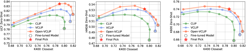
Figure 2: We evaluate the effectiveness of temporal modeling and weight interpolation with a VCLIP B/16 model. Points on each curve represent interpolation ratios of 0.8, 0.7, 0.6, 0.5, 0.4, 0.3, 0.2 and 0.0 from left to right, respectively. The red star marks correspond to our reported main results. We test on the full UCF, HMDB and the first split in (Chen & Huang, 2021) on Kinetics-600.

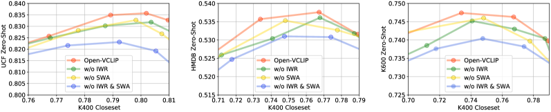
Figure 3: We evaluate the effectiveness of IWR and SWA with a VCLIP B/16 on the full UCF, HMDB and the first split in (Chen & Huang, 2021) on Kinetics-600.

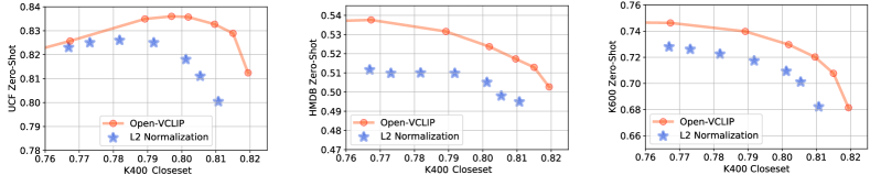
Figure 4: We compare Open-VCLIP with an $\ell_{2}$ regularization imposed on weigths on the full UCF, HMDB and the first split in (Chen & Huang, 2021) on Kinetics-600.

Compared to the baselines, our approach demonstrates significant and consistent improvements in zero-shot video action recognition across various datasets and models, as shown in the last column of Table 4. Taking experimental results on Kinetics-600 as an example, our approach not only avoids the performance drop seen in the “FINE-TUNE” method, but also significantly improves zero-shot recognition. This highlights the effectiveness of our method in effectively using annotated video datasets with limited labels for transfer learning and effectively preventing knowledge from forgetting, offering stable and decent results.

5.3 Discussion and Ablation Studies

The effectiveness of temporal modeling and weight interpolation. We also investigate whether temporal modeling is needed for transferring CLIP to the video domain. To this end, we compare the performance of the CLIP, VCLIP, and Open-VCLIP, represented by green, blue and red curves in Figure 2, respectively. In particular, VCLIP expands the original spatial attention of CLIP to spatial-temporal attention without additional parameters as in Open-VCLIP. The curves illustrate weight interpolations with different mixing coefficients between CLIP and the fine-tuned model. Concretely, the $y$-axis displays the accuracy on the zero-shot video dataset, while the $x$-axis displays accuracy on the fine-tunning dataset, Kinetics-400.

Comparing the tails of the green and blue curves, we see that VCLIP achieves not only better close-set performance, but also better zero-shot performance on all of the three datasets. At the same time, when applying weight interpolation with different ratios, VCLIP achieves better trade-off than CLIP, as evidenced by the fact that the blue curve is always on top of the green curve in Figure 2. This strongly suggests the significant advantages that come with incorporating temporal modeling in the context of zero-shot video action recognition.

Furthermore, the clear margins observed between the red curves and the other curves in Figure 2 show that our proposed solution achieves the best trade-off compared to pure fine-tuning. With the same-level of close-set results, our approach always produces better zero-shot accuracy. In addition, the star marks on the red curves, which correspond to the reported main results in Tables 1, 2 and 3, are always better than the other baseline curves.

IWR v.s. SWA. Our approach is composed of two weight interpolation modules: IWR which is used during training to regularize the fine-tuning process and SWA to improve generalization. We investigate their contributions to the final results in Figure 3. Overall, removing either IWR (green curve) or SWA (yellow curve) from the model leads to significant drops, i.e. the red curve outperforms all other curves, suggesting IWR and SWA are complimentary to each other. Furthermore, we see using only IWR or SWA is able to produce a good zero-shot performance improvement, compared to the results with no interpolation at all.

Table 5: Comparison of zero-shot video-to-text/text-to-video Retrieval performance for various algorithms. “T2VRN” denotes the recall@N of text-to-video retrieval. “V2TRN” denotes the recall@N of video-to-text retrieval.

Method	K400 Tune	$\lambda$	K400	t2vR1	t2vR5	t2vR10	v2tR1	v2tR5	v2tR10
Frozen (Bain et al., 2021)	$\times$	-	-	24.7	46.9	57.2	-	-	-
CLIP (Portillo et al., 2021)	$\times$	-	-	31.2	53.7	64.2	27.2	51.7	62.6
CLIP (our implement)	$\times$	-	57.5	31.1	54.2	63.8	28.9	53.0	64.9
Open-VCLIP	$\checkmark$	0.5	78.9	31.3	54.3	65.6	33.6	59.1	70.0
Open-VCLIP	$\checkmark$	0.7	73.4	33.2	57.1	67.4	34.4	59.8	71.2

Weight regularization during fine-tuning. IWR is conceptually similar to EWC (Kirkpatrick et al., 2017), which penalizes the changes of important parameters for solving previous tasks. However, EWC needs to assess the importance of parameters through historical data which is not feasible to our setting. Instead, we simply constrain the optimization by penalizing the weight changes using an $\ell_{2}$ norm. Concretely, we use the $\ell_{2}$ distance between the updated weights and the original weights as the regularization loss term during training, assigning various weights to the regularization loss term. As shown in Figure 4, our method achieves the best trade-off. Open-VCLIP achieves higher close-set and zero-shot accuracy across all the datasets compared with simply applying an $\ell_{2}$ normalization, demonstrating the effectiveness of Open-VCLIP.

Text-to-Video/Video-to-Text Retrieval Performance. Assessing the model via text-to-video/video-to-text retrieval tasks offers insight into its generalizability within the video domain. We follow the paradigm of training models on Kinetics-400 dataset and testing them on MSR-VTT dataset (Xu et al., 2016), which is a large video description dataset. We firstly report the result of our own implementation using CLIP for retrieval as shown in the third row of Table 5, which is similar to the results in (Portillo et al., 2021). This guarantees fair comparisons. Then, we evaluate Open-VCLIP on MSR-VTT. We find that our text-to-video retrieval (given a text to retrieve the corresponding video) recall is comparable to that of raw CLIP but with a much higher close-set score on K400 (78.9% vs 57.5%). Further increasing the mixing coefficient $\lambda$ improves the text-to-video retrieval performance of Open-VCLIP, surpassing the CLIP baseline by 2%. We also show that the video-to-text retrieval (given a video to retrieve the corresponding text) performance of Open-VCLIP is significantly higher than that of the CLIP baseline, demonstrating the effectiveness of our method in preserving the alignment capability when transferring to video domains.

Comparison with parameter-efficient fine-tuning. Fine-tuning only a part of the weights of a network is an effective approach for adapting the CLIP model to video in a parameter-efficient manner. A noteworthy method that employs this strategy is the ST-Adapter (Pan et al., 2022), which accomplishes effective video classification by training added adapter modules, while keeping the original parameters of the CLIP model frozen. We compare ST-Adapter with our approach. More specifically, ST-Adapter forgoes the text encoder of CLIP, while introducing an additional linear classifier instead. This change prevents the model from being used in zero-shot testing. To circumvent this problem, we incorporate the text encoder of CLIP into our implementation of the ST-Adapter. The results presented in Table 6 illustrates that the ST-Adapter, while preserving the original CLIP weights and only fine-tuning the added adapters, fails to match the performance of our proposed method in zero-shot action recognition. In particular, we observe a marked degradation in the zero-shot performance of the ST-Adapter on the K600 dataset, suggesting that parameter-efficient fine-tuning does not effectively address the issue of catastrophic forgetting.

Table 6: Comparison with parameter efficient fine-tuning method.

Method	UCF	HMDB	K-600
CLIP	74.2	47.6	68.1$\pm$1.0
Fine-tuned VCLIP	79.7	49.2	65.9$\pm$1.0
ST-Adapter	77.3	49.8	60.2$\pm$1.8
Open-VCLIP	83.5	53.2	73.0$\pm$0.8

6 Conclusion

We presented Open-VCLIP, an effective approach that enables CLIP to be transformed to an open-vocabulary video model. Open-VCLIP contains lightweight temporal modeling modules that equip CLIP with the ability to capture spatial and temporal relationships in videos. More importantly, Open-VCLIP is optimized with a carefully designed regularization strategy that strives for generalization to preserve the zero-shot abilities of CLIP. Extensive experiments are conducted and the results demonstrate that Open-VCLIP outperforms state-of-the-art methods with clear margins on zero-shot video action recognition and achieves the best trade-off between close-set and zero-shot video action recognition. One potential limitation is that adversaries could craft membership inference attacks to steal information from the model.

Appendix A Proof

Lemma A.1.

Suppose the image CLIP model was trained on an image-text dataset $D_{\bar{A}}=\{\mathcal{I}_{\bar{A}},\mathcal{T}_{\bar{A}}\}$ with $N$ examples. Then, there exists a diverse video-text dataset $D_{A}=\{\mathcal{V}_{A},\mathcal{T}_{A}\}$ containing $N$ examples where the video CLIP model with original CLIP parameters $\theta_{A}$ is optimal.

Proof.

We denote the large-scale visual-language pretraining dataset used to train CLIP as $D_{\bar{A}}=\{\mathcal{I}_{\bar{A}},\mathcal{T}_{\bar{A}}\}$. To bridge the gap between image and video domains, we extend images in $D_{\bar{A}}$ by repeating frames to create a set of static videos $\mathcal{V}_{A}=\{\mathcal{V}_{i}=[\mathcal{I}_{\bar{A}i},\mathcal{I}_{\bar{A}i},...,\mathcal{I}_{\bar{A}i}]\}^{N}$ and let $\mathcal{T}_{A}=\mathcal{T}_{\bar{A}}$. Videos in $D_{A}=\{\mathcal{V}_{A},\mathcal{T}_{A}\}$ are static and do not provide any additional information for prediction. As a result, $\theta_{A}$ which offers the best results for $D_{\bar{A}}$ is also optimal on $D_{A}$. ∎

References

- Arnab et al. (2021) Arnab, A., Dehghani, M., Heigold, G., Sun, C., Lučić, M., and Schmid, C. Vivit: A video vision transformer. In ICCV, 2021.
- Bain et al. (2021) Bain, M., Nagrani, A., Varol, G., and Zisserman, A. Frozen in time: A joint video and image encoder for end-to-end retrieval. In ICCV, 2021.
- Balaji et al. (2020) Balaji, Y., Farajtabar, M., Yin, D., Mott, A., and Li, A. The effectiveness of memory replay in large scale continual learning. arXiv preprint arXiv:2010.02418, 2020.
- Bertasius et al. (2021) Bertasius, G., Wang, H., and Torresani, L. Is space-time attention all you need for video understanding? In ICML, 2021.
- Bishay et al. (2019) Bishay, M., Zoumpourlis, G., and Patras, I. Tarn: Temporal attentive relation network for few-shot and zero-shot action recognition. arXiv preprint arXiv:1907.09021, 2019.
- Brattoli et al. (2020) Brattoli, B., Tighe, J., Zhdanov, F., Perona, P., and Chalupka, K. Rethinking zero-shot video classification: End-to-end training for realistic applications. In CVPR, 2020.
- Bulat et al. (2021) Bulat, A., Perez Rua, J. M., Sudhakaran, S., Martinez, B., and Tzimiropoulos, G. Space-time mixing attention for video transformer. In NeurIPS, 2021.
- Carreira et al. (2018) Carreira, J., Noland, E., Banki-Horvath, A., Hillier, C., and Zisserman, A. A short note about kinetics-600. arXiv preprint arXiv:1808.01340, 2018.
- Chen & Huang (2021) Chen, S. and Huang, D. Elaborative rehearsal for zero-shot action recognition. In ICCV, 2021.
- Crowson et al. (2022) Crowson, K., Biderman, S., Kornis, D., Stander, D., Hallahan, E., Castricato, L., and Raff, E. Vqgan-clip: Open domain image generation and editing with natural language guidance. In ECCV, 2022.
- Farajtabar et al. (2020) Farajtabar, M., Azizan, N., Mott, A., and Li, A. Orthogonal gradient descent for continual learning. In IJCAI, 2020.
- Gao et al. (2019) Gao, J., Zhang, T., and Xu, C. I know the relationships: Zero-shot action recognition via two-stream graph convolutional networks and knowledge graphs. In AAAI, 2019.
- Gao et al. (2020) Gao, J., Zhang, T., and Xu, C. Learning to model relationships for zero-shot video classification. TPAMI, 2020.
- Ghiasi et al. (2021) Ghiasi, G., Gu, X., Cui, Y., and Lin, T.-Y. Open-vocabulary image segmentation. arXiv preprint arXiv:2112.12143, 2021.
- Ghiasi et al. (2022) Ghiasi, G., Gu, X., Cui, Y., and Lin, T.-Y. Scaling open-vocabulary image segmentation with image-level labels. In ECCV, 2022.
- Hu et al. (2021) Hu, H., Li, A., Calandriello, D., and Gorur, D. One pass imagenet. arXiv preprint arXiv:2111.01956, 2021.
- Ilharco et al. (2022) Ilharco, G., Wortsman, M., Gadre, S. Y., Song, S., Hajishirzi, H., Kornblith, S., Farhadi, A., and Schmidt, L. Patching open-vocabulary models by interpolating weights. arXiv preprint arXiv:2208.05592, 2022.
- Izmailov et al. (2018) Izmailov, P., Podoprikhin, D., Garipov, T., Vetrov, D., and Wilson, A. G. Averaging weights leads to wider optima and better generalization. arXiv preprint arXiv:1803.05407, 2018.
- Jain et al. (2015) Jain, M., Van Gemert, J. C., Mensink, T., and Snoek, C. G. Objects2action: Classifying and localizing actions without any video example. In ICCV, 2015.
- Jia et al. (2021) Jia, C., Yang, Y., Xia, Y., Chen, Y.-T., Parekh, Z., Pham, H., Le, Q., Sung, Y.-H., Li, Z., and Duerig, T. Scaling up visual and vision-language representation learning with noisy text supervision. In ICML, 2021.
- Kay et al. (2017) Kay, W., Carreira, J., Simonyan, K., Zhang, B., Hillier, C., Vijayanarasimhan, S., Viola, F., Green, T., Back, T., Natsev, P., et al. The kinetics human action video dataset. arXiv preprint arXiv:1705.06950, 2017.
- Kim et al. (2021) Kim, T. S., Jones, J., Peven, M., Xiao, Z., Bai, J., Zhang, Y., Qiu, W., Yuille, A., and Hager, G. D. Daszl: Dynamic action signatures for zero-shot learning. In AAAI, 2021.
- Kirkpatrick et al. (2017) Kirkpatrick, J., Pascanu, R., Rabinowitz, N., Veness, J., Desjardins, G., Rusu, A. A., Milan, K., Quan, J., Ramalho, T., Grabska-Barwinska, A., et al. Overcoming catastrophic forgetting in neural networks. PNAS, 2017.
- Kuehne et al. (2011) Kuehne, H., Jhuang, H., Garrote, E., Poggio, T., and Serre, T. Hmdb: a large video database for human motion recognition. In ICCV, 2011.
- Lin et al. (2022) Lin, C.-C., Lin, K., Wang, L., Liu, Z., and Li, L. Cross-modal representation learning for zero-shot action recognition. In CVPR, 2022.
- Liu et al. (2011) Liu, J., Kuipers, B., and Savarese, S. Recognizing human actions by attributes. In CVPR, 2011.
- Mandal et al. (2019) Mandal, D., Narayan, S., Dwivedi, S. K., Gupta, V., Ahmed, S., Khan, F. S., and Shao, L. Out-of-distribution detection for generalized zero-shot action recognition. In CVPR, 2019.
- Mishra et al. (2018) Mishra, A., Verma, V. K., Reddy, M. S. K., Arulkumar, S., Rai, P., and Mittal, A. A generative approach to zero-shot and few-shot action recognition. In WACV, 2018.
- Ni et al. (2022) Ni, B., Peng, H., Chen, M., Zhang, S., Meng, G., Fu, J., Xiang, S., and Ling, H. Expanding language-image pretrained models for general video recognition. In ECCV, 2022.
- Pan et al. (2022) Pan, J., Lin, Z., Zhu, X., Shao, J., and Li, H. St-adapter: Parameter-efficient image-to-video transfer learning. In NeurIPS, 2022.
- Portillo et al. (2021) Portillo, Quintero, J. A., Ortiz-Bayliss, J. C., and Terashima-Marín, H. A straightforward framework for video retrieval using clip. In MCPR, 2021.
- Radford et al. (2021) Radford, A., Kim, J. W., Hallacy, C., Ramesh, A., Goh, G., Agarwal, S., Sastry, G., Askell, A., Mishkin, P., Clark, J., et al. Learning transferable visual models from natural language supervision. In ICML, 2021.
- Rusu et al. (2016) Rusu, A. A., Rabinowitz, N. C., Desjardins, G., Soyer, H., Kirkpatrick, J., Kavukcuoglu, K., Pascanu, R., and Hadsell, R. Progressive neural networks. arXiv preprint arXiv:1606.04671, 2016.
- Shin et al. (2017) Shin, H., Lee, J. K., Kim, J., and Kim, J. Continual learning with deep generative replay. In NeurIPS, 2017.
- Soomro et al. (2012) Soomro, K., Zamir, A. R., and Shah, M. Ucf101: A dataset of 101 human actions classes from videos in the wild. arXiv preprint arXiv:1212.0402, 2012.
- Thengane et al. (2022) Thengane, V., Khan, S., Hayat, M., and Khan, F. Clip model is an efficient continual learner. arXiv preprint arXiv:2210.03114, 2022.
- Wang et al. (2021) Wang, M., Xing, J., and Liu, Y. Actionclip: A new paradigm for video action recognition. arXiv preprint arXiv:2109.08472, 2021.
- Wang et al. (2022) Wang, Z., Lu, Y., Li, Q., Tao, X., Guo, Y., Gong, M., and Liu, T. Cris: Clip-driven referring image segmentation. In CVPR, 2022.
- Wu et al. (2023) Wu, W., Sun, Z., and Ouyang, W. Revisiting classifier: Transferring vision-language models for video recognition. In AAAI, 2023.
- Xing et al. (2022) Xing, Z., Dai, Q., Hu, H., Chen, J., Wu, Z., and Jiang, Y.-G. Svformer: Semi-supervised video transformer for action recognition. arXiv preprint arXiv:2211.13222, 2022.
- Xu et al. (2021) Xu, H., Ghosh, G., Huang, P.-Y., Okhonko, D., Aghajanyan, A., Metze, F., Zettlemoyer, L., and Feichtenhofer, C. Videoclip: Contrastive pre-training for zero-shot video-text understanding. arXiv preprint arXiv:2109.14084, 2021.
- Xu et al. (2016) Xu, J., Mei, T., Yao, T., and Rui, Y. Msr-vtt: A large video description dataset for bridging video and language. In CVPR, 2016.
- Xu et al. (2017) Xu, X., Hospedales, T., and Gong, S. Transductive zero-shot action recognition by word-vector embedding. IJCV, 2017.
- Yin et al. (2020) Yin, D., Farajtabar, M., and Sola, A. L. Continual learning with second-order loss approximation. arXiv preprint arXiv:2006.10974, 2020.
- Zellers & Choi (2017) Zellers, R. and Choi, Y. Zero-shot activity recognition with verb attribute induction. arXiv preprint arXiv:1707.09468, 2017.
- Zheng et al. (2022) Zheng, W., Li, Q., Guo, X., Wan, P., and Wang, Z. Bridging clip and stylegan through latent alignment for image editing. arXiv preprint arXiv:2210.04506, 2022.