Modeling barrier-top fission dynamics in a discrete-basis formalism

Abstract

A configuration-interaction model is presented for the barrier region of induced fission. The configuration space is composed of seniority-zero configurations constructed from self-consistent mean-field wave functions. The Hamiltonian matrix elements between configurations include diabatic and pairing interactions between particles. Other aspects of the Hamiltonian are treated statistically, guided by phenomenological input of compound-nucleus transmission coefficients. In this exploratory study the configuration space is restricted to neutron excitations only. A key observable calculated in the model is the fission-to-capture branching ratio. We find that both pairing and diabatic interactions are important for achieving large branching to the fission channels. In accordance with the transition-state theory of fission, the calculated branching ratio is found to be quite insensitive to the fission decay widths of the pre-scission configurations. However, the barrier-top dynamics appear to be quite different from transition-state theory in that the transport is distributed over many excited configurations at the barrier top.

I Introduction

The theory of fission at a barrier top energies has been one of the few topics in low-energy nuclear physics that has been beyond the purview of the configuration-interaction (CI) framework of modern nuclear theory. In that framework one builds a matrix Hamiltonian in a space of Slater determinants composed of nucleon orbitals, with matrix elements derived from nucleon-nucleon interactions. In this work we construct a CI model of fission dynamics with parameters guided by our present knowledge of the nuclear Hamiltonian. From a computational point of view, this formulation has some of the ingredients of the Generator Coordinate Method (GCM) which has also been applied to fission theory re16 . However, the GCM method treats the dynamics as a Schrödinger equation of a few collective coordinates rather than as a discrete-basis matrix Hamiltonian equation.

The present CI model is too simplified to provide a quantitative theory, but hopefully it is sufficiently realistic to allow qualitative conclusions about the fission dynamics at the barrier. See Refs. be22 ; 388 ; 385 ; ha20 for our previous simplified models to that end. While the model is realistic in that the configurations are built from well-documented energy-density functionals, that space is severely truncated, allowing only neutron excitations in seniority-zero configurations. There are two types of residual interaction that are active in a seniority-zero basis, namely the pairing interaction and an interaction associated with diabatic evolution of the wave function.

In order to make a complete theory of reaction cross sections, the Hamiltonian bridge across the barrier must also be augmented with statistical reservoirs. That includes the configurations that make up the compound nucleus and those that link the bridge states to the final fission channels. They will be treated in a statistical way based on the Gaussian Orthogonal Ensemble (GOE).

The basic physical quantities to be computed are the $\mathcal{S}$-matrix reaction probabilities $\mathcal{T}_{{\rm in},k}$ to capture or fission channels,

$$\mathcal{T}_{{\rm in},k}=\sum_{j\in k}|\mathcal{S}_{{\rm in},j}|^{2}.$$ (1)

Here “in” is the neutron entrance channel, and $k$ = “cap” or “f” is the set of exit channels of a given type. The present model is not detailed enough to calculate the absolute reaction probabilities, but we believe it has enough microscopic input to treat the energy dependence of $\mathcal{T}_{{\rm in},k}$ and some aspects of the branching ratio, defined experimentally as

$$\alpha^{-1}=\frac{\int dE\,\mathcal{T}_{\rm in,f}(E)}{\int dE\,\mathcal{T}_{\rm in,cap}(E)}$$ (2)

where the integral is taken over some experimentally defined energy interval.

In the next three sections below, we present the reaction theory formalism, the construction of the bridge Hamiltonian $H_{\rm bridge}$, and the results of calculations with a full Hamiltonian that links an entrance channel to a set of exit channels. In this paper, we only discuss the barrier-top fission of ²³⁶U, but the formalism is general and can be applied to other nuclei as well.

II Reaction theory formalism

There are several ways to formulate reaction theory in a CI framework. The ones that we have employed are the $\mathcal{S}$-matrix theory leading to the Datta formula da01 , the $K$-matrix formulabertsch2000 , and the direct solution for the wave function. The methods are algebraically equivalent al20 ; al21 . The theory requires two matrices, one for the Hamiltonian of the internal states and one for its couplings to the various continuum channels. The Hamiltonian $H$ is a real matrix of dimension $N_{\mu}$ where $N_{\mu}$ is the number of configurations in the fused system. The other matrix is $W$, a real matrix of dimension $N_{\mu}\times N_{\rm ch}$ composed of reduced-width amplitudes $W_{\mu,i}$ coupling configuration $\mu$ to channel $i$. Here, $N_{\rm ch}$ is the number of channels. The partial width to decay from the state $\mu$ through the channel $i$ is

$$\Gamma_{\mu,i}=2W_{\mu,i}^{2}.$$ (3)

In case the channel couples to more than one state, one needs to consider the full decay matrix associated with the channel,

$$\Gamma_{\mu,\mu^{\prime},i}=2W_{\mu,i}W_{\mu^{\prime},i}.$$ (4)

The basis states constructed by the GCM are not necessarily orthogonal and one also needs the matrix of overlaps $S$ between configurations.

In this work we do not need the $\mathcal{S}$-matrix itself, but only reaction probabilities $\mathcal{T}_{i,j}$ between one channel $i$ and another $j$, as given in Eq. (1) above. They can be conveniently calculated by the trace formula,

$$\mathcal{T}_{i,j}(E)={\rm Tr}\,\left(\Gamma_{i}G(E)\Gamma_{j}G^{\dagger}(E)\right),$$ (5)

where $G(E)$ is the Greens’ function

$$G(E)=\left(H-i\sum_{k}\Gamma_{k}/2-SE\right)^{-1}.$$ (6)

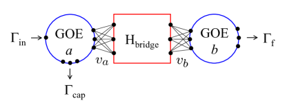
Figure 1: Connectivity of the Hamiltonian for calculating reaction transmission factors. The large circles represent states of the compound nucleus (a) and of the post-barrier configurations (b), both modeled by Hamiltonians of the Gaussian Orthogonal Ensemble (GOE). The rectangular box contains the bridge configurations modeled by an explicit microscopic Hamiltonian. The black dots represent states that connect the different domains of the full Hamiltonian. There is a single entrance channel but multiple exit channels to bound states of the compound nucleus and to states that decay by fission. Couplings to the entrance, capture, and fission channels have associated decay widths given by $\Gamma_{\rm in},\Gamma_{\rm cap}$ and $\Gamma_{f}$, respectively.

III CI model space and Hamiltonian matrix elements

The space of internal states is composed of three sets: those of the compound nucleus, those of the bridge configurations, and those beyond the bridge that ultimately lead to fission. Their Hamiltonian connections are schematically shown in Fig. 1. The dots identify individual configurations at the borders of different sets of states. The circle $a$ denotes the compound-nucleus Hamiltonian as defined by a GOE. We also treat the configurations beyond the barrier (circle b) statistically in the same way. Specific details on their definition and properties are given in Appendix A. The rectangular block represents the bridge states that cross the barrier. They are composed of configurations constructed by a constrained minimization procedure, as is done in the first steps of the GCM. The configurations are linked by parameterized nucleon-nucleon interaction matrix elements. Details are described in the next section below.

The reaction theory also requires decay-width matrices for the entrance channel, the capture channels, and the fission channels. They are depicted in Fig. 1 as $\Gamma_{\rm in},\Gamma_{\rm cap}$, and $\Gamma_{\rm f}$. For the present model, we have good information about the first two widths but no quantitative information about the fission widths on the end.

III.1 Bridge Hamiltonian

We wish to construct the bridge Hamiltonian $H_{\rm bridge}$ as realistically as possible, recognizing that the large dimensions and the number of configuration-interaction matrix elements require severe compromises. The general scheme is easy to describe. The first step is to define a set of reference states along an assumed fission path. These are Slater determinants of nucleon orbitals calculated by constrained density-functional theory. Next one builds a configuration space of particle-hole excitations on each reference state. We call that space a $Q$-block. Finally one computes matrix elements. It should be emphasized that the Slater-determinant basis, also called a Hartree-Fock (HF) basis, is fundamental to the CI approach. It has a certain advantage with respect to quasi-particle bases (called HFB) which require projections to treat specific nuclei.

The bridge Hamiltonian $H_{\rm bridge}$ can be written as

$$H_{\rm bridge}=\sum_{q}H_{q}+\sum_{qq^{\prime}}V_{qq^{\prime}}.$$ (7)

Here $H_{q}$ is the full Hamiltonian within a Q-block and $V_{qq^{\prime}}$ is the interaction Hamiltonian between configurations in different Q-blocks. The next section discusses the selection of reference configurations $q$. The construction of the $H_{q}$ configuration space with its diagonal and off-diagonal matrix elements is given in the sections following that.

The needed computational tools for the diagonal elements of $H_{q}$ are available for several EDF’s, notably the code Skyax for Skyrme functionals skyax and the code HFBaxial for Gogny functionals robledo . In building the reference states, the single-particle potential is assumed to be axially symmetric with good parity. This allows the orbitals as well as the configurations to be classified by quantum numbers for angular momentum about the symmetry axis and parity, $K^{\pi}$ byr18 . To determine the diagonal energies in the Hamiltonian we separate the tasks of setting the absolute energies $E_{q}$ of the reference states and setting the excitation energies $E_{\rm ex}(q\,\mu)$ for configurations $\mu$ within a $Q$-block,

$$\langle q\,\mu|H_{q}|q\,\mu\rangle=E_{q}+E_{\rm ex}(q\,\mu).$$ (8)

For the present model of $H_{q}$, we use the Skyrme energy functional unedf1 unedf1 in the Skyax code. Notice that the effective mass for this interaction is close to unity. The choice is motivated by need to reproduce physical level densities as accurately as possible.

III.1.1 Fission path and reference configurations

Figure 2: The potential energy surface (PES) for the fission path in ²³⁶U  as calculated in the HF and HFB frameworks, shown as solid and dashed lines, respectively. The energy functionals are the Skyrme unedf1 functional (black circles and triangles) and the Gogny D1S functional (blue circles and triangles).

The reference states are placed along a fission path {$q$} defined by some set of constraints, as in the usual GCM. The obvious choice is a single constraint on the elongation of the nucleus; we use the mass quadrupole operator

$$Q=r^{2}P_{2}(\cos\theta)\equiv z^{2}-(x^{2}+y^{2})/2.$$ (9)

The reference states and associated $Q$-blocks will be labeled by an integer $q$ set by the expectation value $\langle Q\rangle$ in units of barns. The energy as a function of the constraint is the so-called potential energy surface (PES). Fig. 2 shows a few PES plots for the nucleus ²³⁶U. In our CI approach we only have discrete points $E_{q}$ on the PES. In the graph the deformation ranges from $q\approx 14$ at the ground state minimum to $q\approx 40$ near the second minimum, with the points spaced by roughly $\Delta\langle Q\rangle\approx 1$ b. The black and blue points were calculated with the Skyrme unedf1 and Gogny D1S EDF’s respectively. The minimizations were carried out in HF and HFB spaces for the circles and squares, respectively. Note that HF PES is far from smooth. There are numerous orbital crossings along the fission path and they are responsible for abrupt changes in slope for both the Gogny and Skyrme EDF, although the locations of the crossings differ. Both HF barriers are much higher than the accepted value between 5 and 6 MeV. As is well known, the calculated barrier height is significantly lowered when the pairing interaction is taken into account. Black squares show the Skyrme PES with neutron pairing included as described in Section III.1.3 below. The lowering is not sufficient to bring the barrier close to the empirical value, and the PES remains bumpy. Ones sees a stronger decrease in barrier height for the Gogny EDF in the HFB treatment, but it is still insufficient to be realistic. Note that the HFB PES is quite smooth. This is likely an unphysical consequence of the HFB space, which inevitably averages over nuclei near the target one.

Since the barrier is unacceptably high we shall rescale the reference state energies $E_{q}^{\rm EDF}$ to bring the PES closer to the empirical. The rescaled energies are given by

$$E_{q}=f_{\rm pes}E_{q}^{\rm EDF}.$$ (10)

Here $E_{q}^{\rm EDF}$ is the reference energy calculated as the difference of energies of the reference state and the ground state at $\langle Q\rangle\approx 14$ b. The scaling parameter $f_{\rm pes}$ is set to $f_{\rm pes}=0.37$ in the $H_{\rm bridge}$ baseline model.

The basis of states in a GCM model need not be orthogonal. This does not impose any conceptual difficulties for the theory but it does add complications. If the reference states are too close together, the wave functions will have large overlaps and the CI calculational framework becomes unstable. On the other hand, the reference states need to be close enough to adequately represent the wave function at all points along the path. A useful measure bo90 ; be19a for setting the spacing of the reference states $|q\,{\rm ref}\rangle$ is the quantity $\zeta$ defined for a chain of $N$ states as

$$\zeta=\sum_{n=0}^{N-1}\Delta\zeta_{n,n+1}$$ (11)

$$\Delta\zeta_{qq^{\prime}}=(-\ln|\langle q\,{\rm ref}|q^{\prime}\,{\rm ref}\rangle|)^{1/2}.$$ (12)

This assumes that the $K^{\pi}$ occupancy of the orbitals is the same all along the chain. It has been shown in a simplified model be22 that spacing the states along the chain by $\Delta\zeta\approx 1$ gives a fairly good approximation to the reaction probabilities. It requires only 5 to 6 reference states along the ²³⁶U fission path from q=18 to q=36, and it is large enough to neglect interactions between $Q$-blocks that are not nearest neighbors.

The definition Eq. (12) fails when the occupation numbers of $K^{\pi}$-partitioned orbitals are different in the two configurations, in which case $\Delta\zeta=0$. This is true for many of the links between reference states. For example, we found that five orbital pair jumps are needed to connect the reference configurations at each end. One can still keep $\zeta$ as a rough measure of distance by extending the configuration space to include the particle-hole excitations in the $Q$-blocks. If the spaces are large enough, all reference state will have a partner in the neighboring $Q$-blocks. To determine the linking, we examine overlaps of the occupied orbitals in the reference configuration with all orbitals of the same $K^{\pi}$ in the other $Q$-block. The desired configuration in the second $Q$-block is the Slater determinant of orbitals with the highest overlaps. We call that configuration the diabatic partner of the reference state. Of course the derived $\Delta\zeta$ for other configurations would vary, but for rough studies the difference should not be important.

Figure 3: Overlap distances of $Q$-blocks along the fission path as defined by Eq. (11). Black dots: a chain of 21 $Q$-blocks separated by roughly $\Delta Q\approx 1$ b. Red dots: the chain of the 6 $Q$-blocks used to construct $H_{\rm bridge}$. Blue dots: an alternative set of 6 $Q$-blocks covering about the same range of deformation.

Fig. 3 shows the $\zeta$ distance function across the barrier for the unedf1 functional with several choices for the reference states, taking the ground state of the left-hand configuration and the diabatic link for the right-hand configuration. Note that the distance between the endpoint configurations is somewhat smaller with the coarser mesh. This is to be expected since the finer mesh path gives more sensitivity to fluctuations in other degrees of freedom. In fact, the adiabatic prescription for defining the path is not optimal for subbarrier fission gu14 ; ha20 .

For the present model, we build the $Q$-blocks on a set of 6 reference states at deformations $q=(18,22,26,29,33,37)$. The configurations beyond those on either side are assumed to be in the statistical reservoirs. We call this the Q6 model. In it, we assume that the diabatic links between the neighboring Q-blocks have the overlap $e^{-(\Delta\zeta)^{2}}$ with the overlap distance of $\Delta\zeta=1$. The overlaps between other configurations, except for those between the same configurations, are simply set to be zero.

III.1.2 $Q$-block spectrum

The spectrum of excited configurations in a $Q$-block is generated in the independent-particle approximation using the orbital energies $\varepsilon_{qi}$ extracted from the same computer code that produced the reference states. The excitation energy is calculated as

$$E_{\rm ex}(q\,\mu)=\sum_{i}\varepsilon_{qi}(\langle q\,\mu|a^{\dagger}_{i}a_{i}|q\,\mu\rangle-\langle q\,{\rm ref}|a^{\dagger}_{i}a_{i}|q\,{\rm ref}\rangle)$$ (13)

in an obvious notation.

Normally the occupied orbitals in the reference state are the lowest ones in the orbital energy spectrum, in which case $E_{\rm ex}$ is always positive. In a few cases the HF minimization fails because the occupation numbers change from one iteration to the next. This is avoided by freezing the $K^{\pi}$ partition after 1500 iterations. In such cases the converged reference state may have one or more empty orbitals below the energy of the highest occupied orbital. Then Eq. (13) gives an unphysical negative energy. This might be corrected by introducing the particle-hole interaction in the Hamiltonian. Rather than complicating the theory this way, we simply ignore the sign in Eq. (13), keeping few with negative energy. This is equivalent to redefining the reference configuration in the PES as the one with the lowest energy in Eq. (13).

To keep the dimensions manageable, we include only neutron excitation in the $Q$-block spaces, Beyond that, we only allow seniority-zero configurations in the neutron spectrum. The occupation numbers are thus the same for both orbitals of a Kramers’ pair. We also restrict the dimension of the space keeping only configurations below an energy $E_{\rm max}$,

$$E_{\rm ex}(q\mu)\leq E_{\rm max}.$$ (14)

Here and in the construction of the full Hamiltonian in Sec. III.2 below we set $E_{\rm max}=4$ MeV.

Table 1 presents some characteristics of the $Q$-blocks constructed in this way. The largest block has a dimension $N_{q}=153$ and total dimension of the bridge configurations is 514. These are small enough for calculations on laptop computers. Notice that the largest dimensions are in the middle region of the barrier. This is consistent with the common understanding that the single-particle density of states at the Fermi level is higher on top of the barrier than elsewhere.

$Q$ (b)	$N_{k}$	$N_{p}$	$N_{p}^{od}$	${N_{db}}^{od}$
18	42	253	416	17
22	97	718	1183	40
26	153	1391	1930	77
29	125	1046	1109	48
33	65	434	322	16
37	32	159
sum	514

Table 1: Dimension $N_{k}$ of Q-blocks on the fission barrier of ²³⁶U based on the unedf1 energy functional and an excitation energy cutoff $E_{\rm cut}=4$ MeV. The column $N_{\rm p}$ shows the number of upper off-diagonal pairing matrix elements in each $Q$-block. Column 4 shows the number of pairing matrix elements between one $Q$-block and the next. Similarly column 5 shows the number of diabatic matrix elements.

Figure 4: Energies of configurations in the Q6 model of $H_{\rm bridge}$. The baseline has been shifted by 1 MeV to take into account the pairing energy in the Q=14 Q-block. Blue line: the scaled PES $E_{q}$; blue dots: diagonal configuration energies $\langle q\,\mu|H_{q}|q\,\mu\rangle$ including $V_{q}$ and the excitation energies $E_{\rm ex}$ of the excited particle-hole configurations; red dots: $Q$-block eigenenergies with pairing interaction included in $H_{q}$; red line: scaled PES with pairing. The cut-off energy of the particle-hole excitation spectrum is $E_{\rm max}=4$ MeV and the pairing strength in the $Q$-block Hamiltonians is $G=0.2$ MeV.

The diagonal spectrum of $H_{\rm bridge}$ is shown in Fig. 4. We use these matrix elements in the full Hamiltonian model treated in Sec. III.2 below.

III.1.3 Interactions

Except for the very lightest systems, microscopic Hamiltonians rely on a reduction of the interaction terms to an effective two-body nucleon-nucleon interaction, see e.g. Ref. ro12 . In this work, we will use simplified interactions whose overall strengths are guided by previous experience. There are two kinds of interaction that can mix configurations in the seniority-zero configuration space. The first is the pairing interaction, which is crucial for promoting spontaneous fission ro14 . It is implicit in the BCS and HFB approximations, but must be explicitly included as a residual interaction in a HF-based configuration space. Following common practice, we parameterize it as the Fock-space operator

$$\hat{v}_{\rm pairing}=-G_{qq^{\prime}}\sum_{i\neq j}a^{\dagger}_{i}a^{\dagger}_{\bar{i}}a_{\bar{j}}a_{j}.$$ (15)

Here $i$ and $\bar{i}$ are time-reversed partner orbitals.

We next determine the interaction strength $G=G_{qq}$ within the $Q$-blocks. The effective strength depends on the size of the configuration space; see Ref. pi05 for numerical studies of that dependence. A typical BCS calculation might be carried out in a full major shell; the observables such as the odd-even binding energy differences can be fitted with a pairing strength $G\approx 25/A$ MeV. This gives $G\approx 0.1$ MeV in the actinide region. However, for our much more limited space the strength should be larger. We choose to set the strength to reproduce the excitation of the first excited $0^{+}$ state in the seniority-zero configuration space of ²³⁶U, $E_{\rm ex}(1)=0.92$ MeV. This yields $G\approx 0.17$ MeV as may be seen in Fig. 5. This is close to the value $G=0.2$ MeV that we use within the $Q$-blocks in the full Hamiltonian.

The pairing strength has to be modified for matrix elements between configurations in different $Q$-blocks. The general formula lowdin for calculating two-body matrix elements in a nonorthogonal CI basis could be used, but it is very time-consuming to carry out. Another formula based on the generalized Wick’s theorem ba69 is fast. However, it requires the two configurations to have a nonzero overlap which is hardly the case for the pairing interaction. In our present model, we will simply assume that overlaps of the configurations attenuate all matrix elements by the same factor,

$$G_{qq^{\prime}}=c\,G.$$ (16)

Here $q$ and $q^{\prime}$ are neighboring Q-blocks and $c=e^{-1}$ is a constant set by the target overlap distance $\Delta\zeta=1$.

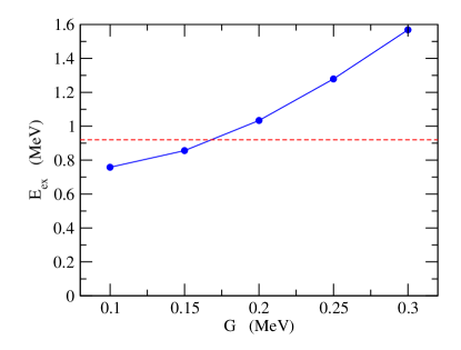
Figure 5: Excitation energy of the first $K^{\pi}=0^{+}$ excited state in the spectrum generated from the ground-state reference state at $Q=14$ b as a function of the pairing strength $G$. Other parameters are the same as used in $H_{\rm bridge}$.

The second kind of interaction matrix element is the coupling to diabatic partner configurations. The diabatic matrix elements are nonzero only for configurations that have large overlaps, so the generalized Wick’s theorem can be applied to calculate them. However, we would still like to make simplifying approximations that make the model calculations more transparent. A convenient functional form for parameterizing the interaction is 388

$$\langle\Psi_{q\mu}|\hat{v}_{db}|\Psi_{q^{\prime}\mu}\rangle=$$ (17)

$$\langle q\mu|q^{\prime}\mu\rangle\left(\frac{1}{2}(E_{q\mu}+E_{q^{\prime}\mu})-h_{2}(\bar{Q})(\Delta\zeta)^{2}\right)$$

where $\bar{Q}=(q+q^{\prime})/2$ and $E_{q\mu}$ is the energy of the configuration including the modified PES. For the present study we will assume a fixed value for the interaction strength, $h_{2}=1.5$ MeV. The motivation for the functional form of Eq. (17) and the choice of the strength parameter $h_{2}$ are discussed in Appendix B. The formula is implemented in the Q6 model with $\langle q\mu|q^{\prime}\mu\rangle=e^{-1}$ for neighboring Q-blocks and $\langle q\mu|q^{\prime}\mu\rangle=0$ when $q$ and $q^{\prime}$ are farther away from each other.

Before going on to the full Hamiltonian we can get a sense of the transmittance of $H_{\rm bridge}$ by calculating the quantity

$$F(E)=\sum_{\mu\in q_{a}}\sum_{\mu^{\prime}\in q_{b}}|(H_{\rm bridge}-S(E-iw))^{-1})_{\mu\mu^{\prime}}|^{2}.$$ (18)

Here $q_{a}$ and $q_{b}$ are the first and last $Q$-blocks in $H_{\rm bridge}$ and $w=0.2$ MeV is an averaging parameter. The result is shown in Fig. 6. There is a large peak just above 4 MeV which is just below the barrier top at 4.6 MeV. There are also smaller peaks below 3.5 MeV that are probably composed of strongly paired configurations. The lowest ones can be identified with the eigenvalues of the $H_{\rm bridge}$ spectrum.

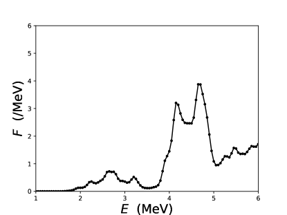
Figure 6: Transmittance of $H_{\rm bridge}$ as measured by Eq. (18). The smearing parameter $w$ is set to be 0.2 MeV.

III.2 The full Hamiltonian

It remains to add the two GOE reservoirs to complete the Hamiltonian depicted in Fig.1. As discussed in Appendix A we have a certain freedom to set the dimension of a GOE reservoir provided the decay widths are modified to keep the transmission factors Eq. (21) fixed. The relevant properties of the entrance and capture channels are well-known experimentally, and we set the transmission coefficients accordingly. Somewhat arbitrarily, we set the dimension of the reservoirs to $N_{\rm GOE}=100$ and the internal interaction strengths in the GOE Hamiltonian to $v=0.1$ MeV. This produces a level density of $\rho_{0}=31.8$ MeV^-1 in the middle of the spectrum. With $\Gamma_{\rm in}=10$ keV, the resulting transmission factor for an $s$-wave neutron entrance channel at $E_{n}=1$ keV is $T_{\rm in}=0.02$. The scaled capture width of the GOE states is $\Gamma_{c}=1.25$ keV. As discussed elsewhere, the fission reaction probability $\mathcal{T}_{{\rm in},f}$ is rather insensitive to the partial widths in reservoir $b$; we have chosen the value $\Gamma_{f}=15$ keV. This is well within the plateau region.

Two sets of interaction matrix elements are still needed to have a complete Hamiltonian, namely those between the GOE reservoirs and $H_{\rm bridge}$. These are placed as depicted in Fig. 1. We parameterize these as Gaussian-distributed random variables with rms strengths $v_{a}$ and $v_{b}$. Each set connects all of the states in the reservoir to all of the configurations in the adjacent $Q$-block. Unfortunately, the strength of these interactions cannot be calculated from microscopic nucleon-nucleon Hamiltonians without a better understanding of the structure of the reservoir states. Thus the overall magnitude of the fission branch is beyond the scope of the model. Nevertheless, the model can still shed light on aspects of the barrier-top dynamics. One aspect is the energy dependence of the reaction probabilities, and another is the importance of the diabatic interaction in the bridge dynamics. These are discussed in the next section. For a baseline model we take $v_{a}=0.02$ and $v_{b}=0.03$ MeV. With these parameters the branching ratio $\alpha^{-1}$ can approach the order of magnitude seen experimentally. Figure 7 shows the reaction probabilities for the Hamiltonian in a small interval of energy. The entrance transmission factor is small enough to show individual compound-nucleus resonances.

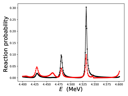
Figure 7: Resonances of the full Hamiltonian at $V_{b}=4$ and $E$ around 3.5 MeV. The black and red points show reaction probabilities for $T_{\rm in,c}$ and $T_{\rm in,f}$ respectively.

IV Reaction probabilities

IV.1 Energy dependence

In this work, we are mainly interested in average reaction probabilities . The averages are obtained by integrating over some interval of energy that includes multiple resonances, and then averaging over the random GOE samples in the Hamiltonian. Fig. 8 shows the reaction probabilities for capture and fission calculated this way. The points were obtained by integrating over an interval of 0.5 MeV and averaging over 400 GOE samples.

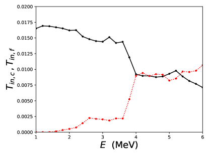
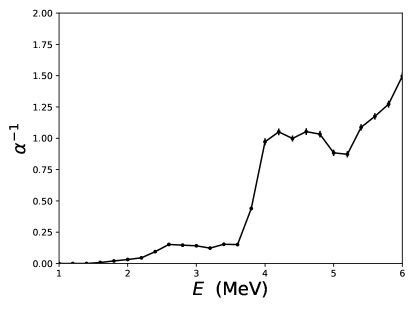
Figure 8: Average reaction probabilities for capture (black circles) and fission (red circles) as a function of energy $E$ are displayed in the upper panel. The branching ration $\alpha^{-1}$ is shown in the lower panel. In the calculation, the two GOE reservoir Hamiltonians are centered at $E$ with fixed decay widths to isolate the energy dependence of transmittance through $H_{\rm bridge}$.

Notice that the total reaction probability remains fairly constant at $\mathcal{T}=\mathcal{T}_{{\rm in},c}+\mathcal{T}_{{\rm in},f}\approx 0.02$ over the entire range plotted. This is required of compound nucleus theory when the entrance channel transmission factor is small compared to the others. Notice also that the fission probability does not increase smoothly at subbarrier energies. This goes against the Hill-Wheeler barrier-penetration formula. There are small windows well below the barrier for transmission that are probably due to the paired $Q$-block ground states. Note also that the reaction probability for fission is monotonically increasing in the energy region shown, contrary to Eq. (18).

IV.2 Branching ratio

The branching ratio $\alpha^{-1}$ (Eq. (2)) as a function of energy $E$ is displayed in the bottom panel of Fig. 8 as a function of energy $E$. The ratio roughly tracks the same irregular increase as that found in the reaction probability shown in the upper panel. It reaches a level of $\alpha^{-1}\approx 1$ at the higher energies. This is less than the experimental ratio of $\approx 3$ in the fission of ²³⁵U by low-energy neutrons. Since the experimental order of magnitude is achieved, the model should be useful for qualitative insights into the transport mechanisms.

We next examine the dependence of the branching ratio on the Hamiltonian parameters. Table 2 presents the results of calculations with different sets of parameters. The calculation for a baseline set of parameters is shown on the top line of the table.

Model	$\Gamma_{c}$	$\Gamma_{f}$	$v_{p}$	$h_{2}$	$v_{a}$	$v_{b}$	$\alpha^{-1}$
base	0.00125	0.015	0.2	1.5	0.02	0.03	$0.95$
A	0.0025						$0.55$
B		0.03					$1.14$
C		0.045					$1.23$
D		0.15					$1.65$
E				3.0			$1.10$
F				0.0			$0.13$
G			0.1				$0.37$
H					0.01		$0.59$
I					0.04		$1.29$
J						0.015	$0.60$
K						0.06	$1.20$

Table 2: Branching ratios calculated with Eqs. (2) and (5) for several sets of energy parameters. Units are MeV. The base parameters are given in the top line. For the other cases only the changes from base are shown in the table. In the calculations, Eq. (2) was evaluated by averaging over an interval from 4.25 to 4.75 MeV. The column shows the mean branching ratio obtained with 400 samples of the compound-nucleus GOE. The resulting in uncertainty limits are about $\pm 0.02$.

It gives $\alpha^{-1}\approx 1.00\pm 0.02$ at 4.5 MeV which is still well below the observed value $\alpha^{-1}\approx 3$ at the physical neutron threshold at 6.5 MeV. One obvious reason is that the excited states of the protons have been left out. Their inclusion might increase the branching ratio. Also, the off-diagonal neutron-proton matrix elements are not active due to the zero-seniority structure of the configurations. However, if no reasonable parameter sets can be found to reproduce the experimental $\alpha^{-1}$ in seniority-zero configuration space, it would be indirect evidence that the space must be extended to include the far more numerous broken-pair configurations.

The other entries in the table indicate the sensitivity of $\alpha^{-1}$ to the Hamiltonian parameters. Lines A-D show the dependence on the decay widths, $\Gamma_{i}$. Entry A is a preliminary check on the model to confirm that an increase in the capture branch produces a corresponding decrease in the fission branch. This is expected in compound nucleus theory when there are many channels for each branch. We see from the B to D entries that the branching ratio is insensitive to the fission branch over a wide range of fission widths. The entries E -K test the dependence on interaction parameters in the Hamiltonian. Entries E and F show that the diabatic interaction cannot be ignored, but the ratio is insensitive to increase beyond the value in the baseline Hamiltonian. One sees from entry G that an error in the pairing strength is likely to propagate to a similar relative error in the branching ratio. This may be contrasted with spontaneous fission, where theoretical lifetimes are very strongly dependent on the pairing strength ro14 . Entries H - K in the table show the effect of changing the matrix elements between $H_{\rm bridge}$ and the GOE reservoirs. As expected, weaker interactions produce smaller fission probability. Doubling $v_{b}$ from its baseline value does not make a significant change in $\alpha^{-1}$, as might be expected from the experience with the fission decay widths. However, there is a substantial decrease when $v_{b}$ is reduced, indicating that the baseline value is at the beginning of a plateau.

V Conclusion and Outlook

The model Hamiltonian in this work introduces for the first time a CI computational framework to describe the many-body dynamics at the fission barrier. A primary conclusion of the study is that the transport appears not to be carried by a small number of internal channels, but rather is diffuse and spread over many barrier topic configurations. If so, it invalidates the transition-state theory that has been accepted uncritically since the earliest work on the subject. However, the model may be deficient in a way that could alter that conclusion. For example, the space of wave functions was generated with time-even constraints which produce only time-even paired wave functions. These have limited band width to transport flux, as was demonstrated in Ref. be22 . If one added time-odd configurations by constraining with a collective momentum operator hizawa2021 ; hizawa2022 as well, the bandwidths would certainly increase.

On the other hand, increasing the space and the scope of the Hamiltonian in other ways is not likely to bring the model closer to the transition-state physics. The pairing interaction acts independently in the neutron and proton subspaces, so inclusion of seniority-zero proton configurations would not make a qualitative change in the excitation function.

The off-diagonal proton-neutron interaction matrix elements may become dominant when broken-pair configurations are included in the CI spacebush92 , and they may work against the collectivity promoted by the pairing interaction. In the limit of large off-diagonal elements with random signs, the dynamics would become diffusive. This probably happens anyway at large excitation energy, but the question remains open for barrier-top energies.

One conclusion points favorably toward future efforts to build a microscopic theory of fission. one sees that the transport properties are determined around the barrier as in the transition-state theory. The branching ratios can thus be calculated without detailed information about the post-barrier Hamiltonian. We called this the “insensitivity property”. The qualitative explanation is very simple: once the system gets past the barrier, it can go so many directions in phase space to get to a fission channel that one can neglect the possibility that it may come back.

We also investigated the relative importance of pairing and diabatic interactions. As expected, the branch ratio is quite sensitive to the pairing interaction strength. In fact the nucleus would not fission at barrier-top energies without pairing being included in some way in the GCM or time-dependent HF approximation scamps2015 ; tanimura2015 . In contrast, the diabatic interaction is not essential for fission, but it substantially enhances the fission branch at a physically relevant strength level.

The prospects for making the model more realistic depend very much on the size of the configuration space in $H_{\rm bridge}$. Some dimensions for extended spaces are shown in Table 3. The costliest numerical task in the reaction theory is the matrix inversion in Eq. (5), but it can be speeded up by taking advantage of its tridiagonal block structure ha20 ; pe08 . Inclusion of proton excitations in the zero-seniority model space requires only $Q$-block dimensions of the order of a few thousands. This is certainly feasible, even with the limited computational power of desk-top computers.

	seniority zero			all $K^{\pi}=0^{+}$
$q$	$n$ only	$p$ only	$n+p$	$n$ only	$n+p$
18	42	23	966	738	$3.2\times 10^{4}$
22	97	46	4462	3088	$3.5\times 10^{5}$
26	153	25	3825	8232	$3.1\times 10^{5}$
29	125	33	4125	5080	$4.3\times 10^{5}$
33	65	18	1170	1455	$1.7\times 10^{4}$
37	32	43	1419	409	$3.9\times 10^{4}$
sum	514	188	15967	19002	$1.1\times 10^{6}$

Table 3: Dimensions of extended spaces to include proton configurations and all seniorities. The cutoff in the configuration spaces is $E_{\rm max}=4$ for both neutrons and protons. The seniority-zero all-nucleon space thus extends up to 8 MeV.

Including all seniorities in the $Q$-block configuration space is much more challenging. The last column in Table III shows the resulting dimensions. The number of $K^{\pi}=0^{+}$ configurations with $E_{\rm max}=4$ MeV is of the order $10^{5}$. With 6 reference states in the bridge region the total dimension is $10^{6}$. To put this in perspective, shell model diagonalizations have been reported for configuration-space dimensions of the order of 10^10-11 shimizu2019 .

Instead of taking brute-force approach to the large configuration spaces, it might be more productive to look for more sophisticated schemes to truncate the active space of states. The theory is already a statistical one due to the GOE reservoirs, but we have not been able to avoid the time-consuming task of numerically sampling the GOE Hamiltonians. Eq. (18) was an attempt to estimate the transmittance of $H_{\rm bridge}$ without the Monte Carlo sampling, but the accord with the full Hamiltonian is not satisfactory. Finally, we need a better understanding of statistical aspects of the interaction matrix elements, since calculating them individually is out of the question.

So far the model does not provide a crisp answer to the question, “How many channels are active in barrier-top fission”? There are at least two ways that one could investigate the question. One is to examine how the probability flux between $Q$-blocks is distributed over the linkages between the block eigenstates: many active links imply many channels. Another way is to examine the resonance width fluctuations in the region of isolated resonances. The fission widths should satisfy the formulava73

$$\nu=\frac{2\langle\Gamma_{f}\rangle^{2}}{\langle\Gamma_{f}^{2}\rangle-\langle\Gamma_{f}\rangle^{2}}$$ (19)

where $\nu$ is the effective number of channels. We intend to investigate this issue in a future publication.

The main codes used in the work will be available on request and later in the Supplementary Material accompanying the published article.

Appendix A GOE model of the statistical reservoirs

This appendix reviews the basic properties of the GOE as a model for the compound nucleus and other statistical reservoirs. It is characterized by two parameters, the dimension of the space $N_{\rm GOE}$ and the strength of the Gaussian-distributed residual interaction $\langle v^{2}\rangle^{1/2}$. We shall also refer to the level density at the center of the distribution, given by

$$\rho_{0}=N_{\rm GOE}^{1/2}/\pi\langle v^{2}\rangle^{1/2}.$$ (20)

For a model of a compound nucleus that can decay by gamma emission (capture) or by fission, there are five additional parameters. They are the decay widths $\Gamma_{\rm in},\Gamma_{\rm cap}$ and $\Gamma_{\rm f}$, together with the number of capture and fission channels, $N_{\rm cap}$ and $N_{\rm f}$. Each channel is paired with a state $\mu$ in the GOE space and given the appropriate decay width $E_{\mu}\rightarrow E_{\mu}-i\Gamma/2$. In compound-nucleus phenomenology the couplings between the channels and the reservoir are better parameterized by transmission coefficients defined as

$$T_{i}\equiv 2\pi\rho_{0}\Gamma_{i}.$$ (21)

We will now set the GOE parameters for the compound-nucleus treatment of the $n+^{235}$U $\rightarrow$ ²³⁶U^∗ reaction. The transmission factor for the entrance channel is taken from the optical model systematics; it is roughly parameterized as

$$T_{\rm in}=2\pi S_{0}E_{n}^{1/2}$$ (22)

where $S_{0}\approx 10^{-4}$ is the strength function (ripl3, , Fig. 10) and $E_{n}$ is the neutron bombarding energy in eV units. For our numerical studies below we take $E_{n}=10$ keV which implies $T_{\rm in}=0.063$. The average gamma decay width of the states in the reservoir is $\Gamma_{\rm cap}\approx 0.04$ eV. The empirical level density associated with an entrance channel is $\rho_{0}\approx 1$ eV^-1, giving

$$T_{\gamma}=2\pi\rho_{0}\Gamma_{\rm cap}\approx 0.25.$$ (23)

We also know that there are many gamma decay channels, so $N_{\rm cap}\gg 1$.

It is not as easy to specify the coupling to the fission channels. For the moment we take the fission width to be $\Gamma_{\rm f}=0.42$ eV as in an example from Ref. BK17 . From the empirical data one can only extract qualitative information about the number of exit channels. As a simple exercise to see how the physical observables depend on the GOE parameters, we take the above parameters plus $(N_{\rm GOE},N_{\rm cap},N_{\rm f})=(50,10,1)$ as a baseline for numerical modeling.

A key attribute of the compound nucleus is that its decay properties are independent of how it was formed, subject to some well-known caveats. The independence is encapsulated in the compound nucleus formula for $\mathcal{T}$:

$$\mathcal{T}_{\rm in,i}=T_{\rm in}\frac{T_{i}}{\sum_{i}T_{i}}.$$ (24)

If the entrance channel width is small compared to other decay widths, the reaction probabilities should sum to $T_{{\rm in}}$:

$$T_{\rm in}\approx\sum_{i}\mathcal{T}_{\rm in,i}.$$ (25)

Table 4 shows how well this works for several treatments of the dimensions $N_{\rm GOE},N_{\rm cap}$ and $N_{\rm f}$.

Model	$N_{\rm GOE}$	$N_{\rm cap}$	$N_{\rm f}$	$\sum_{i}T_{\rm in,i}$	$\alpha^{-1}$
A	50	10	1	0.051	2.03
B	100	10	1	0.050	1.98
C	800	10	1	0.047	2.07
D	50	20	1	0.050	1.99
E	200	20	1	0.049	2.00
F	50	10	2	0.054	3.75
G	50	10	10	0.057	8.57

Table 4: Reaction probability and branching ratio Eq. (2) for GOE models of the $n+^{235}$U compound nucleus reactions. The nominal transmission factors are $(T_{\rm in},T_{\rm cap},T_{\rm f})=(0.063,0.25,2.64)$. The integration interval for calculating the branching ratio covers the center third of the GOE eigenspectrum. Statistical errors associated with the GOE sampling are about 1%.

One sees that Eq. (25) is quite well satisfied and is independent of the dimensional parameters, at least in the range we have computed.

One of the most important physical observables is the branching ratio. The calculated results for GOE model are shown in the last column of Table 4. The dimensions of the GOE space $N_{\rm GOE}$ is varied in the first three lines, which gives one confidence that the enormous size of the physical space is not an obstacle to constructing a practical model. The branching ratio is also nearly independent of $N_{\rm cap}$, provided that the number is large. However, the models F and G show that there is a strong dependence on $N_{\rm f}$. This is a well-known phenomenon and is included in compound-nucleus theory as the Moldauer correction factor va73 ; mo75 .

Appendix B Insensitivity to fission widths

The fission widths in the model are incorporated into the GOE of the post-barrier reservoir. It would be difficult to calculate those widths from a microscopic Hamiltonian. However, we expect that the dimension of the post-barrier reservoir is largely independent of fission exit channels. In that situation the effective decay width is controlled by the coupling to the bridge states 385 . As an example, Fig. 9 shows the structure of a simple GOE model to test the sensitivity to the final-state decay widths. In it, the entrance channel is represented by a chain of two states

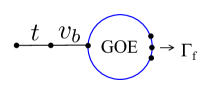
Figure 9: Hamiltonian structure to test the transmission properties of the post-barrier reservoir. The Hamiltonian parameters used in the calculations for Fig. 10 below are: diagonal energies $E_{i}=0$ for the two states $i$ in the entrance channel; $t=1$ for the interaction linking those states; $v_{b}=0.6$ for the interaction connecting the entrance channel to a state in the GOE matrix; $\langle v^{2}\rangle^{-1/2}=0.1$ for the internal interaction strength in the GOE matrix; and $N_{\rm GOE}=100$ and $N_{\rm f}=100$ for the dimension of the GOE Hamiltonian and the number of fission channels.

that couple to the GOE reservoir.

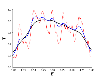
Figure 10: Transmission probability $T_{\rm in,f}$ to decay channels in the post-barrier GOE for a Hamiltonian with the connectivity shown in the previous figure. The decay widths $\Gamma_{f}$ of the GOE states are: 0.05 (dotted red line); 0.2 (dashed blue line); and 0.4 (solid black line). The other Hamiltonian parameters are given in the caption to Fig. 9.

In Fig. 10, the reaction probability $\mathcal{T}$ is plotted as a function of energy for a range of final state widths. One sees that the average $\mathcal{T}$ remains the same over an 8-fold increase in $\Gamma_{f}$. In this situation, the entrance transmission factor is approximately given by

$$T_{\rm in}=(2\pi\rho_{0})^{2}\langle v^{2}\rangle$$ (26)

where $\langle v^{2}\rangle^{1/2}$ is the average interaction matrix element between the entry chain and the reservoir.

We have also made a test of the insensitivity property with the full Hamiltonian. Fig. 11 shows the branching ratio as a function of the assumed fission width $\Gamma_{f}$ of the post-barrier reservoir states. One sees that the $\alpha^{-1}$ varies only by a factor of 1.5 over variation of $\Gamma_{f}$ by a factor of 20. In short, the branching ratio is largely determined by the probability to cross the bridge, rather than the decay rates on the far side.

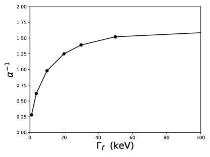
Figure 11: Branching ratio $\alpha^{-1}$ for the full Hamiltonian as a function of fission width $\Gamma_{f}$.

Appendix C Diabatic interaction

In this appendix we examine the diabatic interaction along the $H_{\rm bridge}$ chain to confirm its systematic properties and estimate its overall magnitude. They are calculated with the code GCMaxial robledo which evaluates the matrix elements by the Balian-Brezin formula ba69 . The energy functional employed here is the Gogny D1S functional; its PES was displayed in Fig. 2. For our application, the PES configurations were obtained by the HF minimization procedure. We first demonstrate that Eq. (17) offers

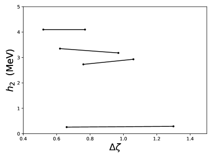
Figure 12: The diabatic matrix element $h_{2}$ given by Eq. (17) for several sets of $(q_{1},q_{2})$ which satisfy $(q_{1}+q_{2})/2=\bar{Q}=25$ b. The Gogny D1S funtional is employed. The quantity is plotted as a function of $\Delta\zeta$ for each set of $(q_{1},q_{2})$.

a reasonable parameterization of the dependence on $\zeta$, as was found in an early study bo90 . In Fig. 12 the diabatic matrix element between configurations at deformations $(q_{1}+q_{2})/2=\bar{Q}=25$ b are calculated as a function of $q_{1}-q_{2}$. The plots show the derived value of $h_{2}$ in Eq. (17) as a function of $\Delta\zeta$. One sees that it is rather insensitive to $\Delta\zeta$. On the other hand, $h_{2}$ has a considerable variation among the different configurations.

In this exploratory study we did not attempt to calculate these matrix elements individually for each diabatic link in the $H_{\rm bridge}$ chain. Instead, we evaluated them for a sample of configurations and used the average for constructing $H_{\rm bridge}$. Fig. 13 shows the results for samples at $\bar{Q}$ between 20 and 30 b, sampling 10 particle-hole configurations at each point. The dots show the averages at each $\bar{Q}$ with the variance shown by the error bars. The overall average $\langle i_{q_{1}}|H|i_{q_{2}}\rangle$ is about 1.5 MeV, and this is the value which we employed in the base parameters shown in Table II.

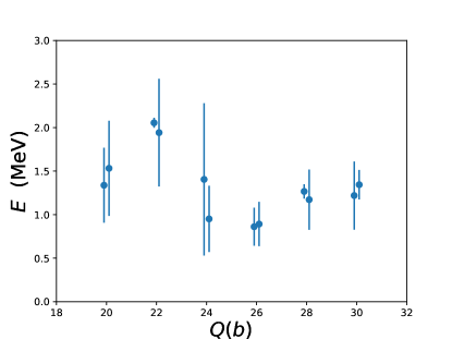
Figure 13: The average and the variance of $h_{2}$, evaluated by sampling 10 particle-hole configurations at each $\bar{Q}$.

References

- (1) D. Regnier, N. Dubray, N. Schunck, and M. Verrière, Phys. Rev. C 93, 054611 (2016).
- (2) G.F. Bertsch and H. Hagino, Phys. Rev. C 105, 034618 (2022).
- (3) K. Hagino and G.F. Bertsch, Phys. Rev. C 105, 034323 (2022).
- (4) G.F. Bertsch and K. Hagino, J. Phys. Soc. Japan 90, 114005 (2021).
- (5) K. Hagino and G.F. Bertsch, Phys. Rev. C 102, 024316 (2020).
- (6) P.S. Damle, A.W. Ghosh, and S. Datta, Phys. Rev. B 64, 201403 (2001).
- (7) G.F. Bertsch, Phys. Rev. C101, 034617 (2000).
- (8) Y. Alhassid, G.F. Bertsch, and P. Fanto, Ann. Phys. (N.Y.) 419, 168233 (2020).
- (9) Y. Alhassid, G.F. Bertsch, and P. Fanto, Ann. Phys. (N.Y.) 424, 168381 (2021).
- (10) S. Yoshida and S. Adachi, Z. Phys. A 325, 441 (1986).
- (11) G. Coló, et al., Phys. Rev. C 50, 1496 (1994), Eq. (B1).
- (12) G.F. Bertsch and W. Younes, Ann. Phys. 403, 68 (2019).
- (13) P.-G. Reinhard, B. Schuetrumpf, and J.A. Maruhn, Comp. Phys. Comm. 258, 107603 (2021).
- (14) L.M. Robledo, private communication.
- (15) G.F. Bertsch, W. Younes, and L.M. Robledo, Phys. Rev. C97, 064619 (2018).
- (16) M. Kortelainen, J. McDonnell, W. Nazarewicz, P.-G. Reinhard, J. Sarich, N. Schunck, M. V. Stoitsov, and S. M. Wild, Phys. Rev. C85, 024304 (2012).
- (17) N. Dubray and N. Regnier, Comp. Phys. Comm. 183, 2035 (2012).
- (18) P. Bonche, J. Dobacaewski, H. Flocard, et al., Nucl. Phys. A 510, 466 (1990).
- (19) G.F. Bertsch, W.Younes, and L.M. Robledo, Phys Rev. C 100, 024607 (2019)
- (20) S. Guiliani, L.M. Robledo and R. Rodriguez-Guzmán, Phys. Rev. C 90, 0543311 (2014).
- (21) R.Roth et al., Phys. Rev. Lett. 109, 052501 (2012).
- (22) R. Rodriguez-Guzmán and L.M. Robledo, Phys. Rev. C 89, 054310 (2014).
- (23) N. Pillet et al., Phys. Rev. C 71, 044306 (2005).
- (24) P. Löwdin, Phys. Rev. 97, 1474 (1955).
- (25) R. Balian and E. Brezin, Il Nouvo Cimento 64, 27 (1969).
- (26) N. Hizawa, K. Hagino, and K. Yoshida, Phys. Rev. C103, 034313 (2021).
- (27) N. Hizawa, K. Hagino, and K. Yoshida, Phys. Rev. C105, 064302 (2022).
- (28) B.W. Busch, G.F. Bertsch, and B.A. Brown, Phys. Rev. C45, 1709 (1992).
- (29) G. Scamps, C. Simenel, and D. Lacroix, Phys. Rev. C92, 011602(R), 2015.
- (30) Y. Tanimura, D. Lacroix, and G. Scamps, Phys. Rev. C92, 034601 (2015).
- (31) D.E. Petersen, et al., J. Comp. Phys. 227, 3174 (2008).
- (32) N. Shimizu et al., Comp. Phys. Comm. Phys. 244, 372 (2019).
- (33) R. Capote et al., Nuclear Data Sheets 110, 3107 (2009).
- (34) G.F. Bertsch and T. Kawano, Phys. Rev. Lett. 119, 222504 (2017).
- (35) R. Vandenbosch and J.R. Huizenga, Nuclear Fission, (Academic Press, New York, 1973), Eq. (IV-4).
- (36) P.A.Moldauer, Phys. Rev. C 11, 426 (1975).