Energy hierarchies governing quarkonium dynamics in Heavy Ion Collisions

Abstract

In this paper, we critically examine hierarchies between energy scales that determine quarkonium dynamics in the quark gluon plasma. A particularly important role is played by the ratio of the binding energy of species ($E_{b}$) and the medium scales; temperature ($T$) and Debye mass ($m_{D}$). It is well known that if these ratios are much larger than one then the dominant process governing quarkonium evolution is dissociation by thermal gluons (gluo-dissociation). On the other hand, if this ratio is much smaller than one then quarkonium dynamics is dominated by screening and Landau damping of the exchanged gluons. Here we show that over most of the evolution, the scale hierarchies do not fall in either limit and one needs to use the full structure of the gluonic spectral function to follow the dynamics of the $Q\bar{Q}$ pair. This has a significant bearing when we follow the quantum dynamics of quarkonia in the medium. The inverse medium relaxation time is also $\sim T$ and if $E_{b}$ is comparable (or larger) in magnitude to $T$, the quantum evolution of $Q\bar{Q}$ is non-local in time within the Brownian approximation.

I Introduction

In the vacuum, the bound states of heavy quarks ($Q$ which can be $b$ or $c$) and anti-quarks ($\bar{Q}$) feature three prominent momentum scales: the heavy quark masses $M$, the inverse relative separation $\frac{1}{r}$, and the binding energies $E_{b}$ (see Ref. N. Brambilla, A. Pineda, J. Soto and A. Vairo (2000) for a comprehensive review). These scales satisfy the hierarchies $M\gg\frac{1}{r}\gg E_{b}$, which justifies non-relativistic treatments of these states. An additional relevant scale for their description is the scale of quantum Chromodynamics ($\Lambda_{QCD}$) which may or may not be somewhat smaller than $E_{b}$ N. Brambilla, A. Pineda, J. Soto and A. Vairo (2000) but can be assumed to be significantly smaller than $1/r$ (especially for $\bar{b}b$ pair). The hierarchy of these scales allows one to integrate out modes at the scale $M$, and $1/r$ systematically, and derive a low energy effective field theory (EFT) valid at the scale $E_{b}$. At the lowest order in $rE_{b}$, the EFT consists of non-relativistic quarks bound by a potential A. Pineda and J. Soto (1998). At higher order, the theory features interactions mediated by gluons of wavelength $1/E_{b}$. Effects of higher order terms are suppressed by positive powers of $rE_{b}$, where factors of $r$ can be seen as arising from a long wavelength expansion of the fields. This framework is called pNRQCD N. Brambilla, A. Pineda, J. Soto and A. Vairo (2000).

In a thermal medium at temperature $T$, new scales appear which govern the dynamic properties of quarkonia in the medium. It was pointed out in a classic paper  T. Matsui and H. Satz (1986) that the screening of the $Q\bar{Q}$ interaction on an inverse length scale $m_{D}$ could lead to the “melting” of the bound states. Moreover, later on, it was realized that scattering between bound states and the thermal constituents of the medium plays a major role in the dissociation of the quarkonium states. This leads to the generation of the imaginary part of the quarkonium potential in a thermal medium Laine et al. (2007). Additionally, absorption of thermal gluons in the medium could lead to gluo-dissociation G. Bhanot and M. E. Peskin (1979). It was shown N. Brambilla, J. Ghiglieri, A. Vairo and P. Petreczky (2008) that pNRQCD naturally incorporates processes leading to gluo-dissociation Peskin (1979); G. Bhanot and M. E. Peskin (1979) as its dynamical degree of freedom that includes low energy gluonic degrees of freedom (and other light degrees of freedom if any) in addition to the wavefunctions of $Q\bar{Q}$ pair. The corresponding emergent scale $\Gamma\sim{1}/{\tau_{R}}$ (where $\tau_{R}$ is the relaxation time of quarkonia) is related to the dynamics of inelastic interactions of $\bar{Q}Q$ with the medium. Furthermore, $E_{b}$ and $\frac{1}{r}$ might themselves be modified from their vacuum values by these thermal effects.

Two medium scales that play a role in quarkonium dynamics in the quark gluon plasma (QGP) are $T$ and $m_{D}$. In the weak coupling limit, there is a hierarchy between $m_{D}$ and $T$ Braaten and Pisarski (1990). In this regime the coupling $g$ is small and $m_{D}\sim gT\ll T$. However, for the temperatures of interest ($150-500$ MeV), lattice results suggest that $m_{D}/T\sim 2$ Kaczmarek et al. (2004). Using $2\pi T$ as the relevant energy scale Brambilla et al. (2021) at which $\alpha_{s}$ is computed also gives similar values of $g$.

This implies that in this regime leading order weak coupling expressions in $g$ are not quantitatively reliable. For example, it is known that the higher order corrections to the momentum diffusion coefficient are larger than the leading order value S. Caron-Huot and G. D. Moore (2008). However, non-perturbative calculations of some relevant dynamical processes is still challenging and weak-coupling calculations are still useful. An important result in weak-coupling was obtained in Ref. Laine et al. (2007) which showed that the potential between quark-antiquark pair is complex at finite $T$.

Such weak-coupling calculations have given insight into the problem and results from these calculations can be used to obtain estimates for experimental observables of interest: for example $R_{AA}$ in heavy ion collisions (HIC).

Many such calculations have been attempted to address the phenomenology of quarkonium states in the QGP (see Ref. Andronic et al. (2016) for a review). For approaches using a medium-modified $T$-matrix approach see Refs. L. Grandchamp, R. Rapp and G. E. Brown (2004); R. Rapp and H. van Hees (2010); X. Zhao and R. Rapp (2011); Emerick et al. (2012); Zhao et al. (2013); Du et al. (2017a); X. Du and R. Rapp (2019). Gluo-dissociation as the dominant mechanism for dissociation has been used in Refs. F. Brezinski and G. Wolschin (2012); F. Nendzig and G. Wolschin (2013); J. Hong and H. Su Lee (2019). For approaches based on the complex potentials derived by Laine et al. (2007) see Refs. Michael Strickland (2011); M. Strickland and D. Bazow (2012); Margotta et al. (2011); Krouppa et al. (2015, 2018, 2019). For approaches based on Schrödinger-Langevin equation see Refs. R. Katz and P. B. Gossiaux (2016); P. B. Gossiaux and R. Katz (2016, 2017). Quarkonia at high $p_{T}$ have been explored in Refs. R. Sharma and I. Vitev (2013); Aronson et al. (2018); Y. Makris and I. Vitev (2019). For quantum dynamics in weak coupling see Refs. Kajimoto et al. (2018); Brambilla et al. (2017, 2018); Islam and Strickland (2020); Sharma and Tiwari (2020).

In this paper, we will focus on bottomonia and use leading order expressions for the gluon polarization tensor. But we will not assume $m_{D}/T$ is small. While this is not a formal expansion in $g$ but might better capture some important qualitative dynamical properties of the QGP. This has been used in other papers for open heavy flavor Moore and Teaney (2005).

The next question is how the thermal scales compare to the scales associated with bound states. Clearly, $M\gg T$ and a non-relativistic treatment is applicable for quarkonia slowly moving in the medium. For bottomonia, the values of $1/r$ are comparable to $\sim 1$GeV A. Mocsy and P. Petreczky (2007) and we will assume that $1/r\gg T$ and hence use pNRQCD to describe the system. However, we do not assume that the hierarchy between $1/r$ and the screening mass $m_{D}$ is so strong that we can ignore the screening of the $Q\bar{Q}$ potential when calculating quarkonium properties in the medium. In practice, we see that the effect of screening on the $\Upsilon(1{\rm{S}})$ wavefunction is small, but the $\Upsilon(2{\rm{S}})$ and $\Upsilon(3{\rm{S}})$ states are affected by screening.

On the other hand, there is no clear separation between $E_{b}$ and $m_{D},T$ (FIG. 4 below). Moreover, their relative order depends on the species and can change as the medium cools down as it evolves. In this paper, we will take all three to be of the same order. Therefore, a non-relativistic treatment is still applicable. However, the integration of modes from $1/r$ to $E_{b}$ includes thermal effects.

Here we would like to point out that further assuming scale separations between $E_{b}$, $m_{D}$, and $T$ can allow us to write simpler EFTs assuming specific choices of these hierarchies. These have been investigated in detail in a series of papers N. Brambilla, J. Ghiglieri, A. Vairo and P. Petreczky (2008); Brambilla et al. (2010, 2011, 2013). Our goal in this paper is to avoid assuming a clear separation between the three scales. In specific regimes where the separations exist, our results will clearly reduce to results from Brambilla et al. (2010, 2013). However, we shall see that in a wide range of parameters, physics lies in an intermediate regime where clear separations do not exist.

To do this we use the full perturbative form of the gluon spectral function. We include contributions from the transverse and longitudinal gluons both in the Landau damping (LD) regime and in the space-like regime where gluo-dissociation occurs. This gives a clear framework to include both processes in a unified language and allows us to compare the contributions to decay from the various process. This is the first time the full gluonic spectral function applicable in both kinematic regimes has been used to compute the total decay rates. In our calculation, the singlet wavefunction is approximated to be the instantaneous eigenstate of a lattice inspired thermal potential and hence incorporates screening. For the octet state, the spectrum is fixed by the constraint that at large $r$ the real part of the octet potential approaches the real part of the singlet potential. For the wavefunction, we systematically compare two limiting cases. One where the screening is strong that the potential is flat in $r$ and the other where the screening is very weak. These can be seen as limiting cases of the physical situation where the screening length is comparable to that in the singlet channel Bala and Datta (2021).

The comparison between $E_{b}$ and $T$ is shown in FIG. 4 which clarifies that these two scales are close to each other. The consequence of this is shown in FIG. 7 where we show for the $\Upsilon(1{\rm{S}})$ state gluo-dissociation dominates in a wide temperature region of interest. FIG. 8 shows that for the $\Upsilon(2{\rm{S}})$ state also both contributions are comparable.

Finally, we find that (FIG. 6) the imaginary potential over-predicts the contribution from LD substantially.

The plan of the paper is as follows. In Sec. II we will review the formalism and highlight the assumptions and approximations involved in our method. In Sec. III, we discuss the connection between $EE$ correlator and the momentum diffusion coefficient of heavy quark, particularly, in the static limit. In Sec. IV, we discuss the implementation of the real part of the singlet potential to obtain the singlet wave function at a given T. We also discuss the two extreme cases of complete screening and no screening for octet interactions. Finally, in Sec. V, we discuss our results followed by the conclusion and future directions in Sec. VI.

II Formalism 

pNRQCD N. Brambilla, A. Pineda, J. Soto and A. Vairo (2000) is an EFT for bound states of quarkonia. In vacuum, it relies on the hierarchy of scales $M\gg\frac{1}{r}\gg E_{b}$. The scale separation $M\gg\frac{1}{r}$ ensures that the $Q$ and $\bar{Q}$ are non-relativistic, and $\frac{1}{r}\gg E_{b}$ means that the interactions between $Q$ and $\bar{Q}$ (at leading order in $1/M$) can be written as potentials.

One can think of it as a two-step process where relativistic dynamics of $Q$ and $\bar{Q}$ are integrated out first, to obtain NRQCD at scales $1/r$ Bodwin et al. (1995). If $\frac{1}{r}\gg T,m_{D}$, the energies corresponding to the thermal scales is much smaller than the relative momentum between $Q\bar{Q}$ ($\sim 1/r$) then NRQCD at this scale is unaffected by $T,m_{D}$, and hence this theory is the same as the theory in vacuum Bodwin et al. (1995).

The pNRQCD lagrangian is obtained by integrating out modes from $1/r$ to $E_{b}$. The structure of the EFT is governed only by the symmetries and the particle content of the theory. In the rest frame of $Q\bar{Q}$ in vacuum, this theory has been extensively studied N. Brambilla, A. Pineda, J. Soto and A. Vairo (2000).

While the medium introduces a new vector $u^{\mu}$ associated with the medium rest frame which can lead to additional operators in the lagrangian Brambilla et al. (2011, 2013), we only consider the case where the quarkonium is (nearly) at rest in the medium, and hence the form of the lagrangian is unchanged from that in vacuum. The lagrangian is of the form

$$\begin{split}\mathcal{L}&=S^{\dagger}\bigg{(}i\partial_{t}+\frac{\nabla^{2}}{M}-V_{s}(r)\bigg{)}S\\ &+O^{\dagger}\bigg{(}i\partial_{t}+\frac{\nabla^{2}}{M}-V_{o}(r)\bigg{)}O\\ &+gV_{A}(r)[S^{\dagger}r\cdot EO+O^{\dagger}r\cdot ES]\\ &+gV_{B}(r)[O^{\dagger}r\cdot EO+O^{\dagger}Or\cdot E]+\cdot\cdot\;.~{}\end{split}$$ (1)

Here $S(O)$ is the singlet (octet) wavefunction in the relative coordinate between $Q$ and $\bar{Q}$. $V_{s}(V_{o})$ is the $Q\bar{Q}$ potential in the singlet (octet) channel. $M/2$ is the reduced mass.

The lagrangian (Eq. 1) is obtained by systematically performing a multipole expansion which encodes the factorization of wavelengths of the order of $1/E_{b}$ compared to the short distance $r$. The dots represent higher order terms in this expansion.

The low energy coefficients (LEC’s) $V_{A}(r)$, $V_{B}(r)$ are $1$ at leading order in perturbation theory and are expected to be close to $1$ at a short distance. In our paper, we will take them to be $1$. The other input to the theory are the potentials, $V_{s}(r)$ and $V_{o}(r)$. If $E_{b}\sim T,m_{D}$, then the integration of modes from $1/r$ to $E_{b}$ is affected by the medium and hence the functional forms of $V_{s}(r)$ and $V_{o}(r)$ is different from their forms in vacuum. If the $Q$ and $\bar{Q}$ can be treated as static (for example if their mass is so high that their kinetic energy can be ignored), then one can run the integration of modes all the way to zero energy. It is well known that in this limit $V_{s}$ and $V_{o}$ are complex Laine et al. (2007); N. Brambilla, J. Ghiglieri, A. Vairo and P. Petreczky (2008). The real and imaginary parts of the static potentials have been calculated in weak coupling limit Laine et al. (2007); N. Brambilla, J. Ghiglieri, A. Vairo and P. Petreczky (2008); Akamatsu (2013). Moreover, we also expect that non-perturbative contributions to the potential are substantial especially for the excited states of bottomonia, because while $1/r$ is large compared to $\Lambda_{QCD}$ the hierarchy is not very strong. Additionally, neither $E_{b}$ nor $T$ are much larger than $\Lambda_{QCD}$ and hence the medium itself at this scale is strongly coupled.

Both the real and imaginary parts of $V_{s}$ Rothkopf et al. (2012); Burnier et al. (2015); Petreczky (2012); Bala and Datta (2020); Bala et al. (2022) and $V_{o}$ Bala and Datta (2021) have been computed non-perturbatively on the lattice.

Let us note that the static calculation gives the $Q\bar{Q}$ potential under the assumption that $E_{b}$ is the smallest scale in the problem and the kinetic energies of the $Q$ and $\bar{Q}$ are negligible. However, if $E_{b}$ and $T$ are comparable, one needs to go beyond the static approximation. In this case the thermal losses can not be captured by an imaginary potential.

In this work we assume that the real part of the potential at scale $E_{b}$ is captured by the static value. Thus, we take the real part of the potentials to be in the range considered by lattice inspired potentials Islam and Strickland (2020). On the other hand to estimate losses due to thermal process, we compute the imaginary part of the singlet self energy diagram in the multipole expansion. The key assumption here is that in the pNRQCD lagrangian (Eq.1) at scale $\sim E_{b}$, the imaginary part of the potential is small and losses predominantly arise from dynamics at scales $\sim E_{b}$. The advantage of this approach is that it captures finite frequency effects of thermal excitation due to the medium. However, this approach misses finite frequency effects in the real parts of the self-energy. These corrections will change the energy of the singlet states and similarly for the octet state and hence change the binding energy of the singlet states. However, the effect of this contribution on the decay rate of the singlet state is higher order in the multipole expansion ($r^{4}$ instead of $r^{2}$) and can be safely ignored in our calculation.

Finally, we assume that the octet state, once formed, decoheres rapidly and can no longer lead to a reformation of the singlet state. In quantum calculations Brambilla et al. (2017); Miura et al. (2019); Sharma and Tiwari (2020) these processes can be taken into account but this is beyond the scope of our paper.

Figure 1: Cut diagrams contributing to the decay width. Single solid line is for singlet and double lines for octet. The gluon line corresponds to a dressed gluon.

With this setup, let us start from a singlet state. The dissociation is given by the imaginary part of the singlet self-energy correction. The corresponding diagram is shown in FIG. 1. Here, the gluon line is resummed and gets contributions both from LD which arises from the imaginary part of the gluon self-energy and pole of the gluon propagator. In FIG.1, gluon momentum ($k_{0}$,${k}$) is directed inward at the first vertex and octet momentum ($q_{0}$,${q}$) is directed outward from the same vertex. The incoming momentum of the singlet is $p_{\mu}=q_{\mu}-k_{\mu}$.

In order to calculate the imaginary part of the singlet self-energy, we follow the cutting rules at the finite temperature are given in Refs. Kobes (1991); Kobes and Semenoff (1986). There are two cut diagrams as shown in FIG. 1 . Following the cut rules and implementing appropriate propagator for each cut diagram, the imaginary part of the self-energy reads as

$$\Im\Sigma_{11}(p_{0},p,r)=\frac{g^{2}C_{F}}{6}r_{i}\bigg{(}\int\frac{d^{4}k}{(2\pi)^{4}}\bigg{\{}\rho_{o}\theta(q_{0})(\theta(-k_{0})$$

$$\qquad+f(|k_{0}|))[k_{0}^{2}\rho_{jj}(k_{0},k)+k_{j}^{2}\rho_{00}(k_{0},k)]\bigg{\}}$$

$$+\int\frac{d^{4}k}{(2\pi)^{4}}\bigg{\{}\rho_{o}\theta(-q_{0})(\theta(k_{0})+f(|k_{0}|))$$

$$\times[k_{0}^{2}\rho_{jj}(k_{0},k)+k_{j}^{2}\rho_{00}(k_{0},k)]\bigg{\}}\bigg{)}r_{i}.$$ (2)

To avoid this lengthy expression, from here onwards, we use the following shorthand notation for the above equation

$$\Im\Sigma_{11}(p_{0},p,r)=r_{i}\hat{\cal{O}}(p_{0},p,r)r_{i}.$$ (3)

In Eq. 2, $C_{F}$ ($=4/3$) is color factor. $\rho_{00}(k_{0},k)$ and $\rho_{jj}(k_{0},k)$ are gluon spectral functions that are discussed in the next section. $p_{\mu}=(p_{0},{\bf{0}})$ is the four-momentum of the incoming singlet state and $\rho_{o}$ is the tree level $Q\bar{Q}$ spectral function in the octet channel which can be obtained from the octet propagator (see Eq. 1)

$$G(q_{0})=\frac{1}{q_{0}-\nabla^{2}/M-V_{o}}.$$ (4)

Hence,

$$\begin{split}\rho_{o}&=2\pi\delta(k_{0}+p_{0}-\hat{q}_{0}),\;\;{\rm{where}}\\ \hat{q}_{0}&=V_{o}+\frac{\nabla^{2}}{M}\;.\end{split}$$ (5)

To proceed further we need information about the temporal and spatial gluonic spectral functions, $\rho_{00}$ and $\rho_{ii}$, which we discuss below.

II.1 Gluon-polarization tensor

In this section, we review the well known expressions for the gluon polarization tensor Kapusta and Gale (2006) that are essential inputs to the evaluation of the imaginary part of quarkonium self-energy.

The general form of the gluon self-energy is given as

$$\Pi_{\mu\nu}(k_{0},k)=P^{L}_{\mu\nu}\Pi_{L}(k_{0},k)+P^{T}_{\mu\nu}\Pi_{T}(k_{0},k),$$ (6)

where $P^{L}_{\mu\nu}(P^{T}_{\mu\nu})$ are longitudinal (transverse) projection operators and $\Pi_{L}(\Pi_{T})$ are component of the gluon self-energy along these directions. In order to evaluate quarkonium decay width using Eq. 3, we need the imaginary part of the gluon propagator. This may come from the pole of the propagator in the region of phase space where the imaginary part of the gluon self-energy is zero, and from the region where the imaginary part of the gluon self-energy is finite. The pole contribution is non-vanishing in the limit $k_{0}>k$, and the latter contribution that requires the real and imaginary parts of the gluon self-energy is finite when $k_{0}<k$ Kapusta and Gale (2006). Below we discuss various components of the gluon self-energy.

Let us first consider the regime $k_{0}<k$ (space-like). This we call the Landau damping regime.

The gluon loop contribution to the imaginary part of the longitudinal component of the gluon self-energy is given as

$$\Im\Pi^{g}_{L}(k_{0},k) = \frac{g^{2}N}{4\pi k}\int_{\frac{k+k_{0}}{2}}^{\infty}dq\,q^{2}\,\bigg{(}2+\frac{k^{4}}{4q^{4}}-\frac{k^{2}}{q^{2}}\bigg{)}$$ (7)

$$\times (f(q-k_{0})-f(q))\,\theta(k-k_{0}),$$

where $N=3$ and $f(q)$ is Bose-Einstein distribution function. Let us note that with an expansion in $k_{0}/T$ in the distribution function and by taking the limit $k\ll q$, Eq.7 goes to its hard thermal loop (HTL) counterpart.

Similarly, The quark loop contribution with $N_{f}$ (light) quark flavors to the imaginary part of the longitudinal component of the gluon self-energy is given as

$$\Im\Pi_{L}^{f}(k_{0},k) = \frac{g^{2}N_{f}}{2\pi k}\int dq\,\bigg{(}q^{2}-\frac{k^{2}}{4}\bigg{)}\,(\tilde{f}(q-k_{0})$$ (8)

$$- \tilde{f}(q))\,\theta(k-k_{0}),$$

where $\tilde{f}(q)$ is Fermi-Dirac distribution function. The total imaginary part of the longitudinal gluon self-energy can be obtained by summing Eqs. 7 and 8.

The real part of the longitudinal component of the self-energy is

$$\Re\Pi_{L}(k_{0},k)=m_{D}^{2}\bigg{(}1-\frac{k_{0}}{2k}\log\bigg{|}\frac{k+k_{0}}{k-k_{0}}\bigg{|}\bigg{)},$$ (9)

where $m_{D}^{2}=\frac{g^{2}T^{2}}{3}\big{(}N+\frac{N_{f}}{2}\big{)}$. In obtaining Eq. 9, we have dropped terms of the order of $k_{0}/T,k/T$. These terms are important when $k_{0},k\gtrsim T$ but we drop these terms because of the following reason. The exact forms of these higher order terms depend on the gauge (for eg. see  Kapusta and Gale (2006)) while Eq. 9 is the HTL form and is gauge invariant Braaten and Pisarski (1990). This expression is valid for both $k_{0}>k$ and $k_{0}<k$. Moreover, from Eq. 3 it is clear that the contribution to $\Im\Sigma$ from $k_{0},k\gg T$ is exponentially suppressed and hence making this approximation will not cause a significant error in our result.

Similarly, for the transverse gluon, the imaginary contributions to the gluon self-energy are,

$$\!\!\!\!\Im\Pi^{g}_{T}(k_{0},k) = \frac{g^{2}N}{2\pi k}\int_{\frac{k+k_{0}}{2}}^{\infty}dq\,\bigg{[}q^{2}\bigg{(}1-\frac{k^{2}}{2q^{2}}\bigg{)}^{2}-\frac{k^{2}}{4}$$

$$\times \!\!\bigg{(}\!2\!-\!\frac{k^{2}}{2q^{2}}\!\bigg{)}^{2}\bigg{]}\!(f(q\!-\!k_{0})\!-\!f(q))\theta(k\!-\!k_{0}),$$

and,

$$\Im\Pi_{T}^{f}(k_{0},k) = \frac{g^{2}N_{f}}{8\pi k}\int_{\frac{k+k_{0}}{2}}^{\infty}dq\,\bigg{(}2q^{2}+\frac{k^{2}}{2}\bigg{)}$$ (11)

$$\times (\tilde{f}(q-k_{0})-\tilde{f}(q))\,\theta(k-k_{0}).$$

The real part of the transverse component of the gluon self-energy is

$$\!\!\!\Re\Pi_{T}(k_{0},k)=\frac{m_{D}^{2}}{2}\bigg{(}\frac{k_{0}^{2}}{k^{2}}-\frac{k_{0}(k_{0}^{2}-k^{2})}{2k^{3}}\log\bigg{|}\frac{k+k_{0}}{k-k_{0}}\bigg{|}\bigg{)}.$$ (12)

Let us now consider the regime $k_{0}>k$ (time-like). This we call the pole regime. In this regime, the imaginary part of $\Pi_{L}$ and $\Pi_{T}$ are zero and the real parts are as above. At order $g^{3}$ the widths of these modes are finite Kapusta and Gale (2006); Bellac (2011) but we ignore this in our calculation.

Now we can calculate the gluon spectral function which goes in Eq. 3. Below we discuss it for both time-like and space-like gluons.

II.2 Gluon spectral functions

The general form of the gluon spectral function in a medium reads as

$$\rho_{\mu\nu}(k_{0},k)={{P}}^{L}_{\mu\nu}\rho_{L}(k_{0},k)+{{P}}^{T}_{\mu\nu}\rho_{T}(k_{0},k).$$ (13)

Here $\rho_{L}(k_{0},k)=D^{R}_{L}(k_{0},k)-D^{A}_{L}(k_{0},k)$ is the longitudinal component of the spectral function and $D^{R(A)}_{L}$ is longitudinal component of resummed retarded (advanced) gluon propagator. Similarly, one can obtain the transverse component of the spectral function ($\rho_{T}$) by using $\rho_{T}(k_{0},k)=D^{R}_{T}(k_{0},k)-D^{A}_{T}(k_{0},k)$. Below we discuss the form of these spectral functions for both $k_{0}>k$ as well as $k_{0}<k$.

For $k_{0}<k$ (LD), we use the gluon self energies (shown in the previous section) to write the resummed gluon propagator and obtain

$$\rho_{L}(k_{0},k)=\frac{2\Im\Pi_{L}(k_{0},k)}{(k^{2}+\Re\Pi_{L}(k_{0},k))^{2}+(\Im\Pi_{L}(k_{0},k))^{2}},$$ (14)

where $\Re\Pi_{L}(\Im\Pi_{L})$ is sum of both gluon and quark contributions.

Similarly, the transverse component of the spectral function can be written as

$$\!\rho_{T}(k_{0},k)\!=\!\frac{2\Im\Pi_{T}(k_{0},k)}{(k_{0}^{2}\!-\!k^{2}\!+\!\Re\Pi_{T}(k_{0},k))^{2}\!+\!(\Im\Pi_{T}(k_{0},k))^{2}}.$$ (15)

It is worth mentioning here that the above form of the spectral functions reproduces the momentum diffusion coefficients obtained within the kinetic theory framework in Ref. Moore and Teaney (2005).

For $k_{0}>k$ the gluon propagator is simply a pole. The quarkonium dissociation in this regime is due to the absorption of a gluon from thermal medium. This process is known as gluo-dissociation in the literature. In the limit $k_{0}\gg T$, the spectral function is given by the imaginary part of free gluon retarded propagator and gluo-dissociation in this case has been studied in Refs. Brambilla et al. (2011); Sharma and Tiwari (2020) However, for realistic situations one needs to take full resummed propagator. Thus, similar to Eq. 13 the general form of the spectral function reads as

$$\rho^{p}_{\mu\nu}(k_{0},k)={\cal{P}}^{L}_{\mu\nu}\rho_{L}^{p}(k_{0},k)+{\cal{P}}^{T}_{\mu\nu}\rho_{T}^{p}(k_{0},k),$$ (16)

where $p$ stands for pole. The longitudinal spectral function in this regime is given by

$$\rho_{L}^{p}(k_{0},k)=2\pi\delta(k^{2}-\Re\Pi_{L}(k_{0},k))\;.~{}$$ (17)

The transverse spectral function is given by

$$\rho_{T}^{p}(k_{0},k)=2\pi\delta(k_{0}^{2}-k^{2}-\Re\Pi_{T}(k_{0},k)).~{}$$ (18)

The imaginary part of $\Sigma_{11}$ gets contribution from both Eqs. 13 and 16. While in the low frequency limit, LD gives the dominant contribution, pole contributions are significantly large in the intermediate and high frequency limit. The overall pole contribution merges with their free spectral function counterpart at an asymptotically large frequency. This we show in FIG. 3.

III Connection with the momentum diffusion coefficient 

In this section, we relate Eq. 3 with the standard definition of the momentum diffusion coefficient in terms of the electric field correlator which is given as J. Casalderrey-Solana and D. Teaney (2006); C. H. Simon and G. D. Moore (2008)

$$\!\!\!\!\kappa=\!\frac{g^{2}}{3N}\!\!\int_{-\infty}^{\infty}\!\!\!\!\!dt\,\text{Tr}\langle U\!(-\infty,\!t)E_{i}(t)U\!(t,\!0)E_{i}(0)U\!(0,\!-\infty)\rangle,$$ (19)

where $U$ is the Wilson line in the fundamental representation, $E_{i}=\partial_{i}A_{0}-\partial_{0}A_{i}$ is the color electric field and trace over color degrees of freedom. In Eq. 19, the infinite integration limit represents the zero frequency limit of the correlator. For the leading order results, one needs to replace the Wilson lines by identity (i.e., $U=\mathds{1}$) to obtain

$$\kappa = \frac{g^{2}C_{F}}{3}\lim_{k_{0}\rightarrow 0}\int d\bar{}\hskip 1.00006pt^{3}k\,k^{2}\,\langle A_{0}(k_{0},k)A_{0}(0,0)\rangle$$ (20)

$$= \frac{g^{2}C_{F}}{3}\lim_{k_{0}\rightarrow 0}\int d\bar{}\hskip 1.00006pt^{3}k\,k^{2}(1+f(k_{0}))\rho_{L}(k_{0},k),~{}$$

for more details see Refs.Moore and Teaney (2005); C. H. Simon and G. D. Moore (2008); Francis et al. (2015a).

It is useful to compare this quantity (Eq. 20) to the expression Eq. 3. Imposing the condition $q_{0}>0$ in Eq. 3 and performing energy integration in Eq. 2 using the energy delta function we rewrite the imaginary part of the singlet self-energy as

$$\begin{split}\Im\Sigma_{11}(k_{0})=\frac{g^{2}r^{2}C_{F}}{6}\times&\\ \int d\bar{}\hskip 1.00006pt^{3}kf(k_{0})&\Bigl{[}k_{0}^{2}\rho_{ii}(k_{0},k)+k^{2}\rho_{00}(k_{0},k)\Bigr{]},\end{split}$$ (21)

where $k_{0}=p_{0}-q_{0}$. For future use, we define a quantity

$$\tilde{\kappa}(k_{0})=\frac{2(\Im\Sigma_{11}(k_{0})|_{\text{pole}}+\Im\Sigma_{11}(k_{0})|_{\text{LD}})}{r^{2}}.$$ (22)

A single heavy quark, traversing through the thermal medium, gets uncorrelated random kicks from the medium constituents that give rise to $\kappa$. However, for quarkonium bound state, not only scattering but also absorption of thermal gluons contribute to the dissociation. The latter process is kinematically forbidden for a single heavy quark. Therefore, in the frequency regime where gluo-dissociation dominates $\tilde{\kappa}$ is not the same as $\kappa$. However, in the static limit where dissociation via scattering (i.e., LD) is dominant, the two coefficients defined in Eqs. 19 and 22 seem identical, at the leading order. We have checked that the LD part of $\tilde{\kappa}$ agrees with the one obtained in Ref. Moore and Teaney (2005).

We note that at higher order there is no reason for these two coefficients to be identical. The reason is that for quarkonium, chromo-electric field correlator is defined with Wilson lines in the adjoint representation Eller et al. (2019). On the other hand for a single heavy quark, Wilson lines are in fundamental representation.

It is useful to note here that in Eq. 22 if one makes $k_{0},k\ll T$ approximation before integrating over $k$, the integrand is of the HTL form and is ultraviolet (UV) divergent. This is due to the fact that the applicability of the HTL resummation is restricted to the low frequency limit. This divergence can be cured by either using a cutoff $k\sim m_{D}$ or by adding the UV contribution to the integral carefully Brambilla et al. (2013). However, the contribution from Eqs.14 and 15 vanishes in the high frequency limit. Therefore, if we use the imaginary part of the longitudinal self-energy given by Eqs. 7 and 8 and evaluate $\tilde{\kappa}$, the integral is convergent and can be computed numerically which we do next.

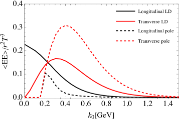
Figure 2: Various contributions to scaled $\langle EE\rangle$ correlator as a function of frequency. Here we take $T=0.25$ GeV and $m_{D}=0.5$ GeV.

In FIG. 2, we plot the electric field correlator arising from various contributions that appear in the evaluation of singlet self-energy diagram in FIG. 1 as a function of frequency. Here we take $T=0.25$ GeV and Debye mass $m_{D}=0.5$ GeV. The black curves are for the longitudinal gluon with a solid line for LD and a dashed one for pole contributions. The red curves are for transverse gluon where solid and dashed lines are for LD and pole contributions, respectively. As anticipated, in the small frequency limit the dominant contribution comes from longitudinal gluon Landau damping. In this limit, other contributions are either zero or very small. Pole contributions switch on at a somewhat larger frequency, i.e., $k_{0}\sim 0.2$ GeV. Moreover, the transverse gluon pole contribution is larger (in magnitude) compared to the longitudinal one. Finally, at high frequency, transverse pole contribution dominates and eventually approaches the corresponding free limit.

In FIG. 3, we have plotted $\tilde{\kappa}/T^{3}$ as a function of $k_{0}$. The red (dashed) curve here gets contribution from both $k_{0}<k$ as well as $k_{0}>k$ phase space regions. In the static limit, i.e., $k_{0}\approx 0$, we have checked that $\tilde{\kappa}/T^{3}$ agrees with that in Ref.Moore and Teaney (2005). The black (solid) line is in the free limit which as expected is zero at zero frequency.

It is well known that the perturbative result for $\kappa$ is too low by roughly a factor of $5-10$ than the non-perturbative value Banerjee et al. (2012); Francis et al. (2015b); Banerjee et al. (2022); Brambilla et al. (2022). For example, recent lattice results for $\kappa/T^{3}$ are estimated as Brambilla et al. (2019)

$$1.99<\frac{\kappa}{T^{3}}<2.69\hskip 28.45274pt\text{for}\hskip 14.22636ptT=1.5T_{c},$$

$$1.05<\frac{\kappa}{T^{3}}<2.26\hskip 28.45274pt\text{for}\hskip 14.22636ptT=3T_{c}.$$

For finite $k_{0}$ there are no lattice results available in the literature. Naively, we expect them to be different from the perturbative estimates. Therefore, we expect that our predictions for $R_{AA}$ are underestimated. However, our results capture the qualitative features of relative contributions of pole and LD in the range of temperatures available in HIC. Motivated by lattice QCD calculations of $m_{D}$, we choose $g=2$ Kaczmarek and Zantow (2005); Islam and Strickland (2020).

In the intermediate frequency regime, the peak structure in $\tilde{\kappa}/T^{3}$ is from the transverse pole contribution. Finally, in the high frequency limit, it merges with its free limit counterpart.

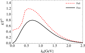
Figure 3: $\tilde{\kappa}/T^{3}$ as a function of frequency for constant coupling $g=2$, $T=0.25$ GeV and $N_{f}=3$. Black (solid) line is the free limit and the dashed (red) is resummed one.

IV Decay width 

At any given temperature $T$, the decay width of a singlet state $|\phi\rangle$ at leading order is given by

$$\Gamma=2\,\langle\phi|\Im\Sigma_{11}|\phi\rangle,$$ (23)

where $\Im\Sigma_{11}$ is given in Eq. 3. Inserting a complete set of octet states $|o\rangle\langle o|$ at the right bracket of Eq. 3, one obtains

$$\Gamma = 2\,\sum_{o}\langle\phi|r\hat{\cal{O}}(p_{0},p,r)|o\rangle\langle o|r|\phi\rangle$$ (24)

$$= 2\,{\cal{O}}(p_{0},p)\sum_{o}\langle\phi|r|o\rangle\langle o|r|\phi\rangle\;,$$

where summation is over all octet states allowed by the selection rule. In operator form ${\cal{O}}(p_{0},p)$ is same as defined in Eq. 3 and now $p_{0}=q_{0}-k_{0}$.

Let us note that the octet state lies in the continuum. $q_{0}$ is the energy of the octet state, which is given by,

$$q_{0}|o\rangle=\bigg{(}V_{o}+\frac{\hat{q}^{2}}{M}\bigg{)}|o\rangle.$$ (25)

One point to note is that momentum conservation implies that the center of mass momentum of the octet state is $-{{k}}$. This implies that the energy of the $|o\rangle$ state has an additional contribution $k^{2}/(4M)$ which should be added to the right hand side of Eq. 25. The value of $k$ is governed by $T$ since it is the region in $k$ space where the gluon spectral function multiplied by the Bose-Einstein distribution function is not exponentially suppressed. In the hierarchy we are working, $E_{b}$ and $T$ are both small scales compared to $M$ and hence quantities of the order of $T^{2}/(4M)$ are suppressed by an extra power of $M$ compared to the right hand side of Eq. 25 and hence can be safely dropped.

IV.1 Modelling the singlet state

To complete the evaluation of Eq. 24, we need the functional form of the singlet state $|\phi\rangle$ as well as octet state $|o\rangle$. Below we discuss the prescriptions to obtain these wave functions.

For a state created in vacuum and “dropped” into the QGP, a natural choice for $|\phi\rangle$ is the wavefunction in vacuum. Further, if the thermal effects are weak then $|o\rangle$ can be taken to as octet states in vacuum. If the initial formation of quarkonia is not affected by the medium (for example if the formation of the quarkonium states occurs on a time scale much shorter than the formation of the QGP) then this is a well motivated model for $|\phi\rangle$ and $|o\rangle$. This picture has been previously used for phenomenology  Park et al. (2007); Sharma and Vitev (2013).

At the LHC and the RHIC, the formation time of the QGP is a fraction of a fm/c and is not substantially larger than the formation time of quarkonia, of the order of $1/E_{b}$. One can expect the formation dynamics of quarkonia to be substantially affected by the medium.

One natural way to include these effects is to start the evolution from a narrow initial $Q\bar{Q}$ state of width $\sim M$ and follow its quantum evolution from very early time Islam and Strickland (2020); Brambilla et al. (2017). In this paper, we do not study the quantum dynamics and this analysis is beyond the scope of the paper. If dissociation can be modelled by the imaginary part of the potential (i.e. in the $E_{b}\ll T$ regime) another possible approach is to assume that the evolution dynamics is slow (adiabatic approximation) and the quarkonium state is initially formed in the eigenstate of the complex potential and at each instant the quarkonium state is in the eigenstate of the complex potential Strickland (2011); M. Strickland and D. Bazow (2012). In this paper, dissociation is calculated using Eq. 3 which can not be captured by a complex potential and hence the adiabatic method is not applicable. We model the effect of the medium on the formation of quarkonia by making the maximal approximation that the initial state and subsequent to formation is determined by the real part of the instantaneous thermal potential Zhao et al. (2013).

More concretely, for the singlet states wavefunction, we use the eigenstates

$$p_{0}|\phi\rangle=\bigg{(}\frac{p^{2}}{M}+V_{s}(r,T)\bigg{)}|\phi\rangle,$$ (26)

where $V_{s}(r,T)$ is the real part of the thermal potential. Here we have subtracted the rest energy from all the $Q\bar{Q}$ states. Similarly, $|o\rangle$ is given by Eq. 25 with $V_{o}$ given by the real part of the octet potential in the thermal medium. In summary, to calculate $|\phi\rangle$ and $|o\rangle$ we need the real parts of the potentials $V_{s}$, $V_{o}$.

	$\Upsilon$(1S)	$\Upsilon$(2S)	$\chi_{b}$(1P)	$\Upsilon$(3S)	$\chi_{b}$(2P)
$M_{M}$	9.46	10.0	9.88	10.36	10.25
$E_{b}$	1.20	0.66	0.78	0.30	0.41
$\langle r^{2}\rangle$	1.42	6.58	4.20	13.68	10.60

Table 1: Binding energies, mass and $\langle r^{2}\rangle$ of various bounds state at $T=0$ using Eq. 27. All dimensions are in GeV. 

For the singlet potential we use the lattice inspired potential which is given by Refs.Dumitru et al. (2009); Islam and Strickland (2020)

$$V_{s}(r,T)\!=\!-\frac{a}{r}(1+m_{D}r)e^{\!-m_{D}r}\!+\frac{2\sigma}{m_{D}}(1\!-e^{\!-m_{D}r})\!-\sigma re^{\!-m_{D}r}\!\!.$$ (27)

The effective coupling $a=0.409$ and the string tension $\sigma=0.21$ GeV² are fixed from the vacuum masses and binding energies (see TABLE 1) with bottom mass $M=4.7$ GeV. Here we take $m_{D}=0$ for obtaining the vacuum spectrum.

For finite $T$ we keep $a$ and $\sigma$ the same as in $T=0$ and $m_{D}=\sqrt{(1+N_{f}/6)}gT$. For $g=2$ Eq.27 gives potentials consistent with those used for bottomonium phenomenology with lattice based potentials Krouppa et al. (2018); Burnier and Rothkopf (2017). The $Q\bar{Q}$ potential in the medium is screened, as a result of which $E_{b}$ becomes smaller with increasing temperature. At sufficiently high temperature the bound state is dissolved T. Matsui and H. Satz (1986). It is worth mentioning that for the 1S state, the wavefunction does not depend on the temperature of the medium up to $T\sim 480$ MeV and it remains approximately the same as that of vacuum Coulombic state while the excited states dissolve earlier A. Mocsy and P. Petreczky (2007).

In FIG. 4, we plot the binding energy of $\Upsilon$(1S), $\Upsilon$(2S) and $\Upsilon$(3S) states as a function of medium temperature. For a given potential, $E_{b}$ is given by $E_{b}=2M-M_{M}+V_{\infty}$, where $M$ is bottom current mass, $M_{M}$ is bound state mass and $V_{\infty}$ is the asymptotic value of real part of singlet potential. The key point we want to highlight in FIG. 4 is that for the temperature range relevant for HICs, the hierarchies $E_{b}\gg T$ or $E_{b}\ll T$ may not be satisfied, at least for 1S and 2S states. It is worth mentioning that $E_{b}$ obtained here agrees with the one in Ref. Du et al. (2017b). On the other hand for higher states, binding energy approaches zero around this temperature and $E_{b}\ll T$.

A consequence of our model is that we can not address the observed phenomenology of the 3S state CMS (2022) as for the central bins $R_{AA}$ for 3S state (in our model) is zero. The key dynamics missing from the classical model are (1) quantum formation dynamics and (2) processes that allow for reformation of bound states which are important for capturing 3S dynamics.

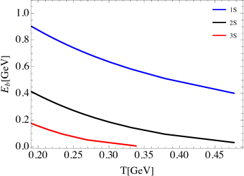
Figure 4: Binding energies for $\Upsilon$(1S), $\Upsilon$(2S) and $\Upsilon$(3S) states as a function of temperature. Here we take constant coupling $g=2$.

IV.2 Modelling the octet state

The octet states are also affected by the thermal medium. At short distances we know that the potential is repulsive Coulombic. In perturbation theory both the real and the imaginary parts of the medium modified octet potential have been computed Akamatsu (2013). Recently, both the real and imaginary parts of the octet potential have also been computed in pure gluonic theory on the lattice Bala and Datta (2021). An important outcome from these papers is that in both perturbative and non-perturbative calculations one finds that at large $r$ the singlet potential approaches the octet potential. This is still an active area of research but the form of the potential for $2+1$ flavor QCD is not yet known.

Based on these considerations, we take two limiting cases for the octet potential. The first is when the screening is strong and one can ignore the octet repulsion at the distance scale of interest and hence

$$V_{o}(r,T)=V_{\infty},$$ (28)

where $V_{\infty}=\frac{2\sigma}{m_{D}}$ is the asymptotic value of singlet potential. In this case, the $|o\rangle$ wavefunctions are the same as the wavefunctions of the free particle but the energy levels start from $V_{\infty}$.

The other limit is where the screening is weak and

$$V_{o}(r,T)\rightarrow C_{F}\frac{{\alpha}}{2Nr}+V_{\infty},$$ (29)

We expect the true physics to be between these two limiting cases.

Finally, the octet potential also has an imaginary piece, which corresponds to the change of the octet state to the singlet state. In this paper, we assume that these processes do not regenerate bound states because the octet states are much broader than the singlet state.

For the repulsive Coulombic potential, the general form of the radial wave function is given as Abramowitz and Stegun (1964)

$$R_{l}(\rho)=\frac{C_{l}}{\rho}\rho^{l+1}e^{i\rho}{}_{1}F_{1}(1+l+i\nu,2l+2,-2i\rho),$$ (30)

where ${}_{1}F_{1}$ is confluent hypergeometric function, $\rho=rp$, $\nu=\frac{1}{8a_{0}p}$ with $a_{0}=\frac{2}{\tilde{\alpha}M}$ as Bohr radius. In this work, we take $a_{0}=1/1.334$ Brambilla et al. (2017).The normalization factor $C_{l}$ in Eq.30 reads as

$$C_{l}=\frac{2^{l}e^{-\frac{\nu\pi}{2}}\sqrt{\Gamma(1+l+i\nu)\Gamma(1+l-i\nu)}}{\Gamma(2+2l)}.$$ (31)

Let us note that for the above form of $C_{l}$, the wavefunction obeys the following form for normalisation

$$\int r^{2}R_{l}(pr)R_{l}(p^{\prime}r)=\frac{(2\pi)^{3}}{p^{2}}\delta(p-p^{\prime}).$$ (32)

With this choice of normalisation, the decay width has the form given in Eqs.36,37 and 39. With the above form of the radial wave function, the general form of the octet wave function can be written as

$$\!\!|o\rangle = 4\pi R_{l}(pr)\sum_{m}Y_{m}^{*l}(\hat{r})Y_{m}^{*l}(\hat{p}).$$ (33)

Here $Y_{m}^{l}$ is spherical harmonics. For the 1P state, replacing $l=1$ in the obove equation and summing over quantum number $m$, the octet wavefunction $|o\rangle$ reads as

$$\!\!\!\!|o\rangle = \sqrt{2\pi}\textbf{p}\cdot\textbf{r}e^{ipr}\sqrt{\frac{\nu(\nu^{2}+1)}{e^{2\pi nu}-1}}{}_{1}F_{1}(2+i\nu,4,-2ipr).$$ (34)

For $s(d)$ states, the wave function can be obtained by replacing $l=0(2)$ in Eq. 33.

In the case of no final state interaction, we take free wave function which in terms of Bessel function is given as

$$|o\rangle=4\pi j_{l}(pr)\sum_{m}Y_{m}^{*l}(\hat{r})Y_{m}^{l}(\hat{p}).$$ (35)

Below we discuss the contribution from the Landau damping and gluon absorption in the decay width.

IV.3 Landau damping contribution

One way to organize the kinematic regimes which contribute to the decay width (Eq. 23) is space-like and time-like. Dissociation (of quarkonia) via scattering of the bound state with the thermal partons occurs when the momentum of the exchanged gluon is space-like. As mentioned, this mechanism is known as LD. It is estimated by taking the resummed propagator for the gluon line in FIG. 1. The LD contribution is dominant when $E_{b}\ll m_{D},T$ N. Brambilla, J. Ghiglieri, A. Vairo and P. Petreczky (2008). The overall contribution is both from the longitudinal as well as transverse gluon. Moreover, in the small $k_{0}$ limit, the longitudinal gluon contribution turns out to be dominant. This is easily understood by noting that while both $\rho_{L}$ and $\rho_{T}$ go as $k_{0}$ at small $k_{0}$, $\rho_{T}$ is multiplied by $(k_{0})^{2}$ in Eq. 3 while $\rho_{L}$ is multiplied by $(k_{i})^{2}$. For $E_{b}\ll m_{D},T$, $k_{0}\ll k$, and hence the longitudinal gluon contribution turns out to be dominant. However, we evaluate both of them numerically and do not drop the transverse contribution.

The explicit expression of $\Gamma_{L}$ for gluonic system is given (see Eq. 24) by,

$$\Gamma_{L} = \!\frac{C_{F}g^{4}N}{6\pi}\!\!\int\!\!d\bar{}\hskip 1.00006pt^{3}pf(k_{0})\!\!\int\!d\bar{}\hskip 1.00006pt^{3}k\frac{k\theta(k-k_{0})}{(k^{2}+\Re\Pi_{00})^{2}+\Im\Pi_{00}^{2}}$$ (36)

$$\times \int_{\frac{k+k_{0}}{2}}^{\infty}dq\,q^{2}\bigg{(}2+\frac{k^{4}}{4q^{4}}-\frac{k^{2}}{q^{2}}\bigg{)}(f(q-k_{0})-f(q))$$

$$\times |\langle\phi|r|o\rangle|^{2}.$$

For finite $N_{f}$, $\Re\Pi_{00}$ and $\Im\Pi_{00}$ gets contribution from the gluon as well as quark loop. Here $p$ is octet momentum and $k_{0}=\frac{p^{2}}{M}-E$ where $E$ is binding energy of the bound state.

Assuming a strong hierarchy between $E_{b}$ and $T$, this can be simplified to the one obtained in Ref.N. Brambilla, J. Ghiglieri, A. Vairo and P. Petreczky (2008).

The transverse gluon contribution arises from the transverse part of the spectral function given in Eq.15. As may be noticed in Eq. 3, for finite $k_{0}$ this term can not be ignored. Moreover, at significantly large $k_{0}$, this term can dominate over the longitudinal gluon contribution. This situation may arise when the hierarchy between $E_{b}$ and medium temperature is not very strong. This can be observed from FIG. 2 that for $k_{0}$ sufficiently large, the transverse contribution to $\Im\Sigma_{11}$ can be larger than the longitudinal. It is also clear that in the kinematic regime where the transverse LD contribution is comparable to the longitudinal LD contribution, the binding energy and the final state interactions can not be ignored in either.

Following the similar prescription as for the case of longitudinal gluon, the contribution to the decay width from the transverse gluon reads as

$$\Gamma_{T} = \!\frac{g^{4}C_{F}N}{3\pi}\!\!\int\!d\bar{}\hskip 1.00006pt^{3}pf(k_{0})\!\!\int\!d\bar{}\hskip 1.00006pt^{3}k\frac{k_{0}^{2}\theta(k-k_{0})}{(k_{0}^{2}-k^{2}-\Re\Pi_{ii})^{2}+\Im\Pi_{ii}^{2}}$$ (37)

$$\times \frac{1}{k}\int_{\frac{k+k_{0}}{2}}^{\infty}\!dq\,\bigg{(}q^{2}\bigg{(}1-\frac{k^{2}}{2q^{2}}\bigg{)}^{2}-\frac{k^{2}}{4}\bigg{(}2-\frac{k^{2}}{2q^{2}}\bigg{)}^{2}\bigg{)}$$

$$\times (f(q-k_{0})-f(q))|\langle\phi|r|o\rangle|^{2}.$$

Total contribution from Landau damping is sum of Eqs. 36 and 37.

IV.4 Pole contribution

In the kinematic regime $E_{b}\gg T$, the dominant contribution to quarkonium dissociation from singlet to unbound octet state occurs by absorbing a time-like gluon from the thermal medium. This process is known as gluo-dissociation Brambilla et al. (2011). For the decay width evaluation, the contribution to the quarkonium self-energy arises from the pole of the gluon propagator. In the free limit, i.e., $T\gg E_{b}$, the medium contribution to the singlet to octet thermal breakup appears in the thermal weight only. However, in the intermediate temperature range, HTL effects also become important and one needs to use resummed propagator. In the HTL resummed propagator, both longitudinal and transverse gluon contribute to the imaginary part of the gluon propagator. After adding both of these contributions and performing $k_{0}$ integration using energy delta function, $\Im\Sigma_{11}$ reads as

$$\Im\Sigma_{11}^{P} = \frac{C_{F}g^{2}r^{2}}{6}f(k_{0})\int\!d\bar{}\hskip 1.00006pt^{3}k\bigg{(}\frac{2k_{0}^{2}\delta(k-k_{0}^{T})}{|{{\partial\Re\Pi_{L}}/{\partial k}}|_{k_{0}^{T}}}$$ (38)

$$+ \frac{k^{2}\delta(k-k_{0}^{L})}{|{{\partial\Re\Pi_{T}}/{\partial k}}|_{k_{0}^{L}}}\bigg{)},$$

where $k_{0}^{T}$ is solution of $k_{0}^{2}-k^{2}-\Re{\Pi_{T}}=0$ and $k_{0}^{L}$ is that of $k_{0}^{2}-\Re{\Pi_{L}}=0$. In the limit $T\gg E_{b}$, Eq. 38 can be solved analytically by making an expansion in the bosonic distribution and replacing the spectral function by the free spectral function. Using Eq. 38, decay width is given as

$$\Gamma_{P} = \frac{C_{F}g^{2}}{3}\int\!\!d\bar{}\hskip 1.00006pt^{3}pf(k_{0})\int\!d\bar{}\hskip 1.00006pt^{3}k\bigg{(}\frac{2k_{0}^{2}\delta(k-k_{0}^{T})}{|{{\partial\Re\Pi_{T}}/{\partial k}}|_{k_{0}^{T}}}$$ (39)

$$+ \frac{k^{2}\delta(k-k_{0}^{L})}{|{{\partial\Re\Pi_{L}}/{\partial k}}|_{k_{0}^{L}}}\bigg{)}|\langle\phi|r|o\rangle|^{2}.$$

The contribution of transverse gluon to the decay width of the bound states is dominant over the longitudinal one. This can be observed from the frequency behavior of $\Im\Sigma_{11}$ shown in FIG. 2. Below we discuss the results obtained for the decay width and $R_{AA}$.

V Results for classical dynamics 

In this section, we discuss the results for $\Upsilon$(1S) and $\Upsilon$(2S) states using the decay width obtained in the previous section. We mainly focus on the relative contributions of pole and LD within the perturbative limit and show the overall effect on $R_{AA}$.

At any given time $t$, the survival probability of a given singlet state can be obtained by using the rate equation

$$\frac{dN(t)}{dt}=-N(t)\sum_{i}\Gamma_{i}(t),$$ (40)

where $N(t)$ is the number of bound states at time $t$ and summation is over the two contributions arising from LD and pole. The total number of states produced after some time $t_{f}$ may be obtained from Eq. 40 and is given as

$$N=N_{0}e^{-\int_{t_{0}}^{t_{f}}\Gamma(t)dt}.$$ (41)

Here $t_{0}$ is the initial time, $N_{0}$ is number of bound states at time $t_{0}$, and $\Gamma(t)=\sum_{i}\Gamma_{i}(t)$.

V.1 Medium model

To calculate $\Gamma$ as a function of time we need a model for the background evolution of the thermal medium. In this paper we use a simple model and take the medium by a Bjorken expanding medium Bjorken (1983) with a temperature

$$T(t)=T(t_{0})\bigg{(}\frac{t_{0}}{t}\bigg{)}^{\frac{1}{3}}.$$ (42)

We are interested in quarkonia with zero rapidity and hence have replaced the proper time with the local time. $T(t_{0})$ is the temperature at a reference proper time $t_{0}$. We take $t_{0}=0.6$ fm which is a little later than the start of hydrodynamics for LHC energies Chang et al. (2016). This is starting time for the quarkonium evolution and is comparable to the formation time for quarkonia. Similar numbers were taken in Ref. Brambilla et al. (2018).

The temperature at time $t_{0}$ depends on the impact parameter or equivalently the centrality. We use centrality bins analogous to the one used in ALICE Adam et al. (2016a). For this purpose, we use the Glauber model (we do not use the Monte-Carlo Glauber model here though we see that the difference between our centrality bins and the bins obtained from the Monte-Carlo Glauber model  Miller et al. (2007) is small) to relate the impact parameter to the number of participants ($N_{part}$) and the number of binary collisions($N_{bin}$). Following ALICE, bins in the observed $dN_{ch}/d\eta$ are related to bins in $N_{part}$ using the relation

$$\frac{dN_{ch}}{d\eta}=\lambda(fN_{bin}+(1-f)N_{part}),$$ (43)

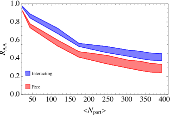
Figure 10: $R_{AA}$ for $\Upsilon(2S)$ state as a function of $<N_{part}>$ for each centrality bin. Color representation is same as FIG.9.

where $\lambda=2.75$ and $f=0.212$ Adam et al. (2016a). With these values of the parameters $\lambda$ and $f$, we quantitatively agree with the centrality dependence of $dN_{ch}/d\eta$ as a function of $N_{part}$ given in FIG.10 of Ref.Abelev et al. (2013). For each centrality bin, we have mentioned the mean value of $N_{part}$ and impact parameter $b$ in TABLE2.

Centrality(%)	Npart	b (fm)	$T_{0}$ (MeV)
0-2.5	393	$2.5$	446	478
2.5-5	363	$3.5$	443	475
5-7.5	334	$5.0$	439	470
7.5-10	307	$7.0$	434	465
10-20	248	$8.7$	420	450
20-30	173	$10.0$	408	437
30-40	116	$11.2$	371	398
40-50	74	$12.2$	317	339
50-60	44	$13.2$	267	286
60-70	23	$14.0$	207	222

Table 2: Mean value of $N_{part}$, impact parameter ($b$) and initial temperature ($T_{0}$) for various centrality bins. $T_{0}$ is temperature at time $t_{0}=0.6$ fm. The left column in $T_{0}$ is for $f=1.462$ and the right one is for $f=1.782$ (see text below Eq. 47).

With $dN_{ch}/d\eta$ in hand for each centrality bin, the initial temperature at $t_{0}$ is obtained by using following prescription Srivastava et al. (2018). The value of $d\mathcal{N}/dy$ is related to the experimentally measured charged particle multiplicity by the relation,

$$\frac{d\mathcal{N}}{dy}=\frac{3J}{2}\frac{dN_{ch}}{d\eta},$$ (44)

where $J=1.12$ is the jacobian for $y$ to $\eta$ transformation Adam et al. (2016b). $\mathcal{N}$ is the multiplicity of the particles produced at the end, $y$ is pseudo-rapidity. The factor $3/2$ in Eq. 44 incorporates the contribution from neutral particles. In order to be consistent within our model, for each centrality bin, we take $dN_{ch}/d\eta$ obtained by using Eq. 43 with the parameters mentioned above.

In the nuclear collision experiments, the number density of partons or entropy is decided by the rapidity distribution of the produced particles. Assuming that initially the system is at chemical equilibrium, and assuming that the entropy does not change during the evolution, we can write the initial parton density as

$$n_{0}=\frac{1}{A_{\perp}t_{0}}\frac{d\mathcal{N}}{dy},$$ (45)

where $A_{\perp}$ is transverse size of the system. We estimate it from the Glauber model for each centrality via Eyyubova et al. (2021)

$$A_{\perp}=4\pi\sqrt{\langle x^{2}\rangle\langle y^{2}\rangle},$$ (46)

where $\langle x^{2}\rangle,\langle y^{2}\rangle$ is size along the transverse directions. A rough estimate of $T_{0}$ can be made from the initial number density assuming a non-interacting QGP. Then, $n_{0}=(\beta_{1}+2\beta_{2})T_{0}^{3}$ with $\beta_{1}=8\pi^{2}/15$ and $\beta_{2}=7\pi^{2}N_{f}/40$ represents equilibrium density for gluon and quark. Plugging it back in Eq.45 along with Eq.44, we obtain the initial temperature at time $t_{0}$ to be

$$T_{0}=\bigg{(}\frac{3J}{2A_{\perp}t_{0}}\frac{dN_{ch}}{d\eta}\frac{1}{\beta_{1}+2\beta_{2}}\bigg{)}^{\frac{1}{3}}.$$ (47)

For $\sqrt{s}=2.76$ TeV, Eq.47 gives $T_{0}\sim 250$ MeV for the most central bin ($0-2.5$%). This is significantly lower than estimates of the temperatures obtained at $t_{0}\approx 0.6$ fm in hydrodynamic simulations Chang et al. (2016). We note that Eq.45 ignores various effects such as particalization, viscous effects, interaction in the QGP, and expansion in the transverse direction. Moreover, losses in the work done by the system during the expansion are also not taken into account. These effects may lead to entropy generation and energy loss restricting the applicability of Bjorken expansion. Thus the initial parton density will be somewhat larger than estimated by Eq. 45. In order to take these losses into account we redefine the initial parton density by multiplying Eq. 45 with a fudge factor ($f$) i.e., $n_{0}=fn_{0}$.

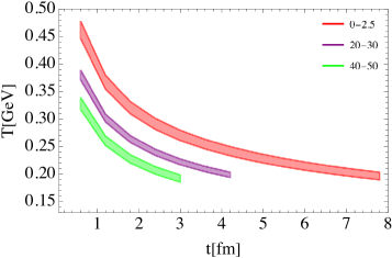
Figure 5: Temperature as a function of time. Red band is for the most central bin and, central and green one are for 20-30% and 40-50% centrality, respectively. Here the initial time $t_{0}=0.6$ fm for all centrality bins. The band here covers upper and lower temperature correspond to two different values of the fudge factor.

This fudge factor is adjusted in such a way that we obtain the initial temperature in the most central bin to range from $T_{0}\approx 450$ MeV ($f=1.46$) to $T_{0}\approx 480$ MeV ($f=1.78$) at $t_{0}=0.6$ fm. For our final results of $R_{AA}$ we provide the band corresponding to these two values of the initial temperatures. While this is a highly simplified model for the background medium, we hope that this band of variation captures important features of its hydrodynamic evolution.

In FIG.5, we show the variation of temperature as a function of time starting with $t_{0}=0.6$ fm till the temperature reaches the final value of 190 MeV.

Finally, for completeness, we also consider the final state feed-down effect, we follow the prescription given in Ref. Islam and Strickland (2020). Therefore, for a given bound states, $R_{AA}$ is given by

$$R_{AA}=\frac{N+\alpha N_{h}}{N_{0}+\alpha N_{0h}},$$ (48)

where $N_{h}$ is number of higher states at the end of evolution and $\alpha$ is feed-down parameter from higher state ($N_{h}$) to the state being considered. Feed-down matrix is given in Eq.(5.2) of Ref.Islam and Strickland (2020). $N_{0}$ is number of states at the initial time $t_{0}$. In the results presented here, for feed-down , we only consider higher states with contributions more than 10%. Thus for $\Upsilon$(1S), we take the contribution from $\Upsilon$(2S), $\chi_{b0}$(1P),$\chi_{b1}$(1P) and $\chi_{b1}$(2P) states. We follow the same for $\Upsilon$(2S) state as well. For more details on feed down see Ref.Islam and Strickland (2020). Below we discuss the results in somewhat more detail.

V.2 Results

In FIG. 6, we compare the decay width (of $\Upsilon$(1S) and $\Upsilon$(2S) states) from Eq. 36 with the (imaginary) potential Mikko Laine (2007) formalism which is extensively used in the literature. In the latter case the decay width is obtained from

$$\Gamma=2\langle\phi|\Im V_{s}(r,T)|\phi\rangle,$$ (49)

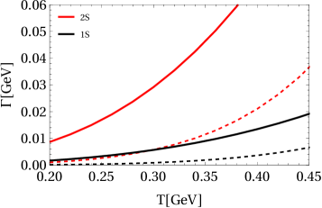
Figure 6: Decay width of 1S (black) and 2S (red) from imaginary potential (solid line) and longitudinal LD (dashed line) given in Eq.36.

where $\Im V_{s}$ is the imaginary part of the singlet potential. In order to be consistent with the $r^{2}$ expansion in Eq. 1, we also make this approximation in the imaginary part of the potential. In this limit, the momentum integration in the potential becomes divergent, limiting its applicability in the small momentum ranges. We therefore put an upper cut off $m_{D}$ to get finite results. The corresponding decay width for $\Upsilon$(1S) and $\Upsilon$(2S) states are shown by the solid line in FIG. 6. In the same figure, we show the decay width obtained from Eq. 36 with $E_{b}=0.6$ GeV (for 1S) and $0.2$ GeV for 2S. As may be noticed, $\Im V_{s}(r,T)$ gives a larger decay width which can be understood as follows.

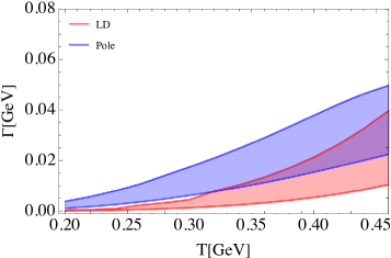
Figure 7: Decay width of the $\Upsilon(1{\rm{S}})$ state as a function of medium temperature. The band corresponds to the free wave function (upper curve) (Eq. 35) and Coloumbic repulsive wavefunction (lower curve) (Eq. 33). Red color band is LD and blue color band is gluo-dissociation.

Eq. 49 assumes the binding energy of the singlet state, and the octet state energy ($q^{2}/M$) of the species is negligible compared to the temperature. This can be seen by inserting a complete set of octet states in Eq. 36. The energy delta function gives $k_{0}=q^{2}/M-E_{b}$. Taking the limit $k_{0}\to 0$, Eq.36 gives the result obtained from the imaginary potential expanded in $r$ to order $2$. We emphasize here that for realistic values, this approximation over-predicts the decay rate. We have checked that if we do not make an expansion in $r$ in the imaginary potential, the decay width turns out to be even larger.

In FIG. 7, we plot the scattering (LD) and gluo dissociation (pole) contributions to $\Upsilon$(1S) state. For $\Upsilon$(2S) we plot the same quantity in FIG. 8. The bands correspond to no screening (Eq. 33) and complete screening (Eq. 35) scenarios. Here we take $E_{b}=0.6$ GeV (for 1S) and $E_{b}=0.2$ GeV (for 2S) which lie in the middle (see FIG. 4) of the binding energies within the temperature range of interest.

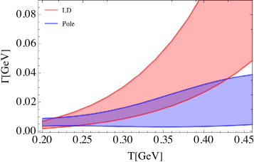
Figure 8: Decay width of the $\Upsilon(2{\rm{S}})$ state as a function of medium temperature. The color conventions are the same as in Fig. 7

It may be observed (from FIG. 4) that the hierarchies $E_{b}\gg T$ or $E_{b}\ll T$ are not very well satisfied for both $1S$ and $2S$ states. One would therefore expect significant contribution from the finite frequency region of FIG. 3. For $\Upsilon$(1S), this may be observed in FIG. 7. As anticipated, with this value of $E_{b}$, pole (blue band) and LD (red band) give somewhat similar contribution for a wide range of temperature.

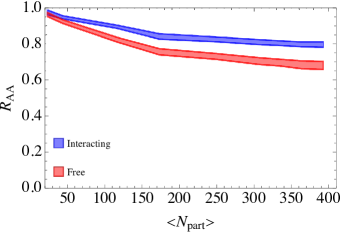
Figure 9: $R_{AA}$ for $\Upsilon(1S)$ state as a function of $\langle N_{part}\rangle$ for each centrality bin. For blue color we take octet potential as vacuum potential and for red color we switch off octet potential assuming complete screening.

Moreover, LD contribution dominates at high temperature. Similarly, for $\Upsilon$(2S) state, pole contribution is larger at temperature $\sim 200$ MeV and at high temperature $\sim 400$ MeV, LD contribution is significantly larger than the pole contribution. This suggest that for $\Upsilon$(2S) dissociation, LD gives dominant contribution.

In FIG. 9, we combine both gluon absorption and scattering processes and plot $R_{AA}$ for $\Upsilon(1S)$ state as a function of $\langle N_{part}\rangle$ for each centrality bin.

For a given centrality, we first evaluate singlet state wave functions at each temperature by solving the Schrodinger equation given in Eq.26. With temperature dependent wave functions at hand, we estimate matrix element i.e., $|\langle\phi|r|o\rangle|^{2}$ (see Eq.36) and obtain corresponding decay width for all processes. Here we use temperature dependent binding energy shown in FIG. 4. Finally, we use Eq. 48 to estimate $R_{AA}$ for a given state. As mentioned earlier, we consider two cases ; (a) when there is no screening in the final state octet interaction (show in blue color)and (b) when octet states are completely screened (shown in red color). Here, upper and lower edge of the band corresponds to the lower and higher initial temperature given in TABLE 2.

Let us note that in the realistic situations, octet potential is neither completely screened nor has form of pure vacuum potential. Therefore, we expect the true value of suppression to lie somewhere between the blue and the red bands. It is evident that the suppression is under-predicted for these states. This may largely be due to the fact that the spectral functions are obtained at the leading order (LO) accuracy. Further improvements of our results require non-perturbative estimate of these spectral functions on lattice which so far have been computed only in the static limit.

VI Conclusion 

In this work, we perform a comprehensive analysis to quantify the relative contributions arising from LD and gluo-dissociation to the $\Upsilon$(1S) and $\Upsilon$(2S) states within leading order perturbation theory for the medium. We assume that the real part of the singlet potential is screened in a thermal medium, and we take lattice motivated real parts of the $Q\bar{Q}$ potential and estimate the binding energy and wave function as a function of $T$ for $\Upsilon$ and $\chi$ states. By comparing the binding energy (shown in FIG. 4) and temperature it can be seen that for the 1S and 2S states both $E_{b}$ and $T$ are comparable to each other (although for the 2S state for $T>300$MeV one could take $T\gg E_{b}$). We, therefore, expect that neither $E_{b}\gg T$ nor $E_{b}\ll T$ hierarchy is strictly satisfied in the interesting range of temperatures for the QGP, at least for 1S and 2S. However, for other higher excited states, $E_{b}\ll T$ seems to be satisfied quite well. For $\Upsilon(3S)$ this can be seen in FIG. 4.

The consequence for the 1S state (and for the 2S in the later stages of the evolution) is that LD can not adequately describe the decay of the state. It is well known that in the static limit i.e., $k_{0}\rightarrow 0$, decay dominantly happens via longitudinal LD which can be captured by an imaginary potential between $Q\bar{Q}$. However, this limit is valid if the binding energy of the quarkonium species is negligible compared to the medium temperature. As discussed in the text below FIG. 6, this also requires the kinetic energy of the octet states to be small. For $E_{b}\sim T$, the full finite frequency region of the spectral function for the chromo-electric field correlator becomes important.

There is a caveat to the above conclusion. The perturbative value of the $k_{0}\rightarrow 0$ value of the chromo-electric spectral function is a factor of $5-10$ times smaller than the non-perturbative value calculated on the lattice. If this enhancement persists till $k_{0}$ values of a few 100 MeV (see FIG. 3) then our conclusion about the relative contribution of the LD and the other contributions will be still be true. However, if the spectral function rapidly drops down towards the perturbative estimate (at $k_{0}\sim$ GeV we expect the leading order perturbative result to be more reliable) then the LD contribution dominates for all the states and the static results can be used to capture the physics of interest. This provides a motivation to study the spectral function at finite frequency non-perturbatively, although it is a difficult problem.

The hierarchy between $E_{b}$ and $T$ ($T$ is related to the inverse of the environment time scale) plays an important role while performing a quantum calculations of quarkonia dynamics within the open quantum system framework. It has been shown Akamatsu (2015, 2022); Brambilla et al. (2017) that if $E_{b}\ll T$ quarkonium system is in the quantum Brownian motion regime and the evolution is local in time. In this case, one can obtain a Lindblad equation for the density matrix evolution for the $Q\bar{Q}$ system. On the other hand if $E_{b}\gtrsim T$ then this proof fails. We show here that this is the case for the $\Upsilon(1\rm{S})$ state throughout the evolution if one considers the state to be an eigenstate of the instantaneous (real) potential. $E_{b}$ is also $\lesssim T$ for the excited states in the early part of the evolution. However, If substantial regeneration of the excited states happens at the later time (low temperature) then the hierarchy $E_{b}\gtrsim T$ might be satisfied. In this regime if a quantum Brownian description of the dynamics is attempted, one might need dynamics that are correlated in time. Although a quantum optical description might become applicable in this case X. Yao and T. Mehen (2019); Yao and Mehen (2021). We do not discuss quantum evolution in this work and leave this for the future.

VII Acknowledgements

We acknowledge support of the Department of Atomic Energy, Government of India, under Project Identification No. RTI 4002. We also thank Saumen Datta and Michael Strickland for valuable discussions.

VIII References

References

- N. Brambilla, A. Pineda, J. Soto and A. Vairo (2000) N. Brambilla, A. Pineda, J. Soto and A. Vairo, Nuclear Physics B 566, 275 (2000).
- A. Pineda and J. Soto (1998) A. Pineda and J. Soto, Nuclear Physics B - Proceedings Supplements 64, 428 (1998), proceedings of the QCD 97 Euroconference 25th Anniversary of QCD.
- T. Matsui and H. Satz (1986) T. Matsui and H. Satz, Phys. Lett. B178, 416 (1986).
- Laine et al. (2007) M. Laine, O. Philipsen, M. Tassler, and P. Romatschke, Journal of High Energy Physics 2007, 054 (2007).
- G. Bhanot and M. E. Peskin (1979) G. Bhanot and M. E. Peskin , Nucl. Phys. B156, 391 (1979).
- N. Brambilla, J. Ghiglieri, A. Vairo and P. Petreczky (2008) N. Brambilla, J. Ghiglieri, A. Vairo and P. Petreczky, Phys. Rev. D 78, 014017 (2008).
- Peskin (1979) M. E. Peskin, Nuclear Physics B 156, 365 (1979).
- Braaten and Pisarski (1990) E. Braaten and R. D. Pisarski, Phys. Rev. D 42, 2156 (1990).
- Kaczmarek et al. (2004) O. Kaczmarek, S. Ejiri, F. Karsch, E. Laermann, and F. Zantow, Finite density QCD. Proceedings, International Workshop, Nara, Japan, July 10-12, 2003, Prog. Theor. Phys. Suppl. 153, 287 (2004), arXiv:hep-lat/0312015 [hep-lat] .
- Brambilla et al. (2021) N. Brambilla, M. A. Escobedo, M. Strickland, A. Vairo, P. Vander Griend, and J. H. Weber, JHEP 05, 136 (2021), arXiv:2012.01240 [hep-ph] .
- S. Caron-Huot and G. D. Moore (2008) S. Caron-Huot and G. D. Moore, Phys. Rev. Lett. 100, 052301 (2008).
- Andronic et al. (2016) A. Andronic et al., Eur. Phys. J. C76, 107 (2016), arXiv:1506.03981 [nucl-ex] .
- L. Grandchamp, R. Rapp and G. E. Brown (2004) L. Grandchamp, R. Rapp and G. E. Brown, Phys. Rev. Lett. 92, 212301 (2004), arXiv:hep-ph/0306077 [hep-ph] .
- R. Rapp and H. van Hees (2010) R. Rapp and H. van Hees, in Quark-gluon plasma 4 (2010) pp. 111–206, arXiv:0903.1096 [hep-ph] .
- X. Zhao and R. Rapp (2011) X. Zhao and R. Rapp, Nucl. Phys. A859, 114 (2011), arXiv:1102.2194 [hep-ph] .
- Emerick et al. (2012) A. Emerick, X. Zhao, and R. Rapp, Eur. Phys. J. A48, 72 (2012), arXiv:1111.6537 [hep-ph] .
- Zhao et al. (2013) X. Zhao, A. Emerick, and R. Rapp, Proceedings, 23rd International Conference on Ultrarelativistic Nucleus-Nucleus Collisions : Quark Matter 2012 (QM 2012): Washington, DC, USA, August 13-18, 2012, Nucl. Phys. A904-905, 611c (2013), arXiv:1210.6583 [hep-ph] .
- Du et al. (2017a) X. Du, M. He, and R. Rapp, Phys. Rev. C96, 054901 (2017a), arXiv:1706.08670 [hep-ph] .
- X. Du and R. Rapp (2019) X. Du and R. Rapp, JHEP 03, 015 (2019), arXiv:1808.10014 [nucl-th] .
- F. Brezinski and G. Wolschin (2012) F. Brezinski and G. Wolschin, Physics Letters B 707, 534 (2012).
- F. Nendzig and G. Wolschin (2013) F. Nendzig and G. Wolschin, Phys. Rev. C 87, 024911 (2013).
- J. Hong and H. Su Lee (2019) J. Hong and H. Su Lee, (2019), arXiv:1909.07696 [nucl-th] .
- Michael Strickland (2011) Michael Strickland, Phys. Rev. Lett. 107, 132301 (2011), arXiv:1106.2571 [hep-ph] .
- M. Strickland and D. Bazow (2012) M. Strickland and D. Bazow, Nucl. Phys. A879, 25 (2012), arXiv:1112.2761 [nucl-th] .
- Margotta et al. (2011) M. Margotta, K. McCarty, C. McGahan, M. Strickland, and D. Yager-Elorriaga, Phys. Rev. D83, 105019 (2011), [Erratum: Phys. Rev.D84,069902(2011)], arXiv:1101.4651 [hep-ph] .
- Krouppa et al. (2015) B. Krouppa, R. Ryblewski, and M. Strickland, Phys. Rev. C92, 061901 (2015), arXiv:1507.03951 [hep-ph] .
- Krouppa et al. (2018) B. Krouppa, A. Rothkopf, and M. Strickland, Phys. Rev. D97, 016017 (2018), arXiv:1710.02319 [hep-ph] .
- Krouppa et al. (2019) B. Krouppa, A. Rothkopf, and M. Strickland, Proceedings, 27th International Conference on Ultrarelativistic Nucleus-Nucleus Collisions (Quark Matter 2018): Venice, Italy, May 14-19, 2018, Nucl. Phys. A982, 727 (2019), arXiv:1807.07452 [hep-ph] .
- R. Katz and P. B. Gossiaux (2016) R. Katz and P. B. Gossiaux, Annals Phys. 368, 267 (2016), arXiv:1504.08087 [quant-ph] .
- P. B. Gossiaux and R. Katz (2016) P. B. Gossiaux and R. Katz, Proceedings, 25th International Conference on Ultra-Relativistic Nucleus-Nucleus Collisions (Quark Matter 2015): Kobe, Japan, September 27-October 3, 2015, Nucl. Phys. A956, 737 (2016), arXiv:1601.01443 [hep-ph] .
- P. B. Gossiaux and R. Katz (2017) P. B. Gossiaux and R. Katz, Proceedings, 16th International Conference on Strangeness in Quark Matter (SQM 2016): Berkeley, California, United States, J. Phys. Conf. Ser. 779, 012041 (2017), arXiv:1611.06499 [hep-ph] .
- R. Sharma and I. Vitev (2013) R. Sharma and I. Vitev, Phys. Rev. C87, 044905 (2013), arXiv:1203.0329 [hep-ph] .
- Aronson et al. (2018) S. Aronson, E. Borras, B. Odegard, R. Sharma, and I. Vitev, Phys. Lett. B778, 384 (2018), arXiv:1709.02372 [hep-ph] .
- Y. Makris and I. Vitev (2019) Y. Makris and I. Vitev, (2019), arXiv:1906.04186 [hep-ph] .
- Kajimoto et al. (2018) S. Kajimoto, Y. Akamatsu, M. Asakawa, and A. Rothkopf, Physical Review D 97, 014003 (2018).
- Brambilla et al. (2017) N. Brambilla, M. A. Escobedo, J. Soto, and A. Vairo, Phys. Rev. D 96, 034021 (2017).
- Brambilla et al. (2018) N. Brambilla, M. A. Escobedo, J. Soto, and A. Vairo, Phys. Rev. D 97, 074009 (2018).
- Islam and Strickland (2020) A. Islam and M. Strickland, JHEP 21, 235 (2020), arXiv:2010.05457 [hep-ph] .
- Sharma and Tiwari (2020) R. Sharma and A. Tiwari, Phys. Rev. D 101, 074004 (2020), arXiv:1912.07036 [hep-ph] .
- Moore and Teaney (2005) G. D. Moore and D. Teaney, Phys. Rev. C 71, 064904 (2005).
- A. Mocsy and P. Petreczky (2007) A. Mocsy and P. Petreczky, Phys. Rev. Lett. 99, 211602 (2007), arXiv:0706.2183 [hep-ph] .
- Brambilla et al. (2010) N. Brambilla, M. Á. Escobedo, J. Ghiglieri, J. Soto, and A. Vairo, Journal of High Energy Physics 2010, 38 (2010).
- Brambilla et al. (2011) N. Brambilla, M. Á. Escobedo, J. Ghiglieri, and A. Vairo, Journal of High Energy Physics 2011, 116 (2011).
- Brambilla et al. (2013) N. Brambilla, M. A. Escobedo, J. Ghiglieri, and A. Vairo, JHEP 05, 130 (2013), arXiv:1303.6097 [hep-ph] .
- Bala and Datta (2021) D. Bala and S. Datta, Phys. Rev. D 103, 014512 (2021), arXiv:2009.00773 [hep-lat] .
- Bodwin et al. (1995) G. T. Bodwin, E. Braaten, and G. P. Lepage, Phys. Rev. D51, 1125 (1995), [Erratum: Phys. Rev.D55,5853(1997)], arXiv:hep-ph/9407339 [hep-ph] .
- Akamatsu (2013) Y. Akamatsu, Physical Review D 87, 045016 (2013).
- Rothkopf et al. (2012) A. Rothkopf, T. Hatsuda, and S. Sasaki, Phys. Rev. Lett. 108, 162001 (2012), arXiv:1108.1579 [hep-lat] .
- Burnier et al. (2015) Y. Burnier, O. Kaczmarek, and A. Rothkopf, Phys. Rev. Lett. 114, 082001 (2015), arXiv:1410.2546 [hep-lat] .
- Petreczky (2012) P. Petreczky, Journal of Physics G: Nuclear and Particle Physics 39, 093002 (2012).
- Bala and Datta (2020) D. Bala and S. Datta, Phys. Rev. D 101, 034507 (2020), arXiv:1909.10548 [hep-lat] .
- Bala et al. (2022) D. Bala, O. Kaczmarek, R. Larsen, S. Mukherjee, G. Parkar, P. Petreczky, A. Rothkopf, and J. H. Weber (HotQCD), Phys. Rev. D 105, 054513 (2022), arXiv:2110.11659 [hep-lat] .
- Miura et al. (2019) T. Miura, Y. Akamatsu, M. Asakawa, and A. Rothkopf, (2019), arXiv:1908.06293 [nucl-th] .
- Kobes (1991) R. Kobes, Phys. Rev. D 43, 1269 (1991).
- Kobes and Semenoff (1986) R. L. Kobes and G. W. Semenoff, Nucl. Phys. B 272, 329 (1986).
- Kapusta and Gale (2006) J. I. Kapusta and C. Gale, Finite-Temperature Field Theory: Principles and Applications, 2nd ed., Cambridge Monographs on Mathematical Physics (Cambridge University Press, 2006).
- Bellac (2011) M. L. Bellac, Thermal Field Theory, Cambridge Monographs on Mathematical Physics (Cambridge University Press, 2011).
- J. Casalderrey-Solana and D. Teaney (2006) J. Casalderrey-Solana and D. Teaney, Phys. Rev. D74, 085012 (2006), arXiv:hep-ph/0605199 [hep-ph] .
- C. H. Simon and G. D. Moore (2008) C. H. Simon and G. D. Moore, Journal of High Energy Physics 2008, 081 (2008).
- Francis et al. (2015a) A. Francis, O. Kaczmarek, M. Laine, T. Neuhaus, and H. Ohno, Phys. Rev. D 92, 116003 (2015a), arXiv:1508.04543 [hep-lat] .
- Eller et al. (2019) A. M. Eller, J. Ghiglieri, and G. D. Moore, Phys. Rev. D 99, 094042 (2019), [Erratum: Phys.Rev.D 102, 039901 (2020)], arXiv:1903.08064 [hep-ph] .
- Banerjee et al. (2012) D. Banerjee, S. Datta, R. Gavai, and P. Majumdar, Phys. Rev. D 85, 014510 (2012).
- Francis et al. (2015b) A. Francis, O. Kaczmarek, M. Laine, T. Neuhaus, and H. Ohno, Phys. Rev. D 92, 116003 (2015b).
- Banerjee et al. (2022) D. Banerjee, R. Gavai, S. Datta, and P. Majumdar, (2022), arXiv:2206.15471 [hep-ph] .
- Brambilla et al. (2022) N. Brambilla, V. Leino, J. Mayer-Steudte, and P. Petreczky (TUMQCD), (2022), arXiv:2206.02861 [hep-lat] .
- Brambilla et al. (2019) N. Brambilla, V. Leino, P. Petreczky, and A. vairo (TUMQCD), in 37th International Symposium on Lattice Field Theory (Lattice 2019) Wuhan, Hubei, China, June 16-22, 2019 (2019) arXiv:1912.00689 [hep-lat] .
- Kaczmarek and Zantow (2005) O. Kaczmarek and F. Zantow, Phys. Rev. D 71, 114510 (2005), arXiv:hep-lat/0503017 .
- Park et al. (2007) Y. Park, K.-I. Kim, T. Song, S. H. Lee, and C.-Y. Wong, Phys. Rev. C 76, 044907 (2007), arXiv:0704.3770 [hep-ph] .
- Sharma and Vitev (2013) R. Sharma and I. Vitev, Phys. Rev. C 87, 044905 (2013), arXiv:1203.0329 [hep-ph] .
- Strickland (2011) M. Strickland, Phys. Rev. Lett. 107, 132301 (2011), arXiv:1106.2571 [hep-ph] .
- Dumitru et al. (2009) A. Dumitru, Y. Guo, A. Mocsy, and M. Strickland, Phys. Rev. D 79, 054019 (2009), arXiv:0901.1998 [hep-ph] .
- Burnier and Rothkopf (2017) Y. Burnier and A. Rothkopf, Phys. Rev. D 95, 054511 (2017), arXiv:1607.04049 [hep-lat] .
- Du et al. (2017b) X. Du, M. He, and R. Rapp, Nucl. Phys. A 967, 904 (2017b), arXiv:1704.04838 [hep-ph] .
- CMS (2022) CMS, Observation of the meson and sequential suppression of states in PbPb collisions at , CMS-PAS-HIN-21-007 (2022).
- Abramowitz and Stegun (1964) M. Abramowitz and I. A. Stegun, Handbook of Mathematical Functions with Formulas, Graphs, and Mathematical Tables, ninth dover printing, tenth gpo printing ed. (Dover, New York, 1964).
- Bjorken (1983) J. D. Bjorken, Phys. Rev. D 27, 140 (1983).
- Chang et al. (2016) N.-b. Chang et al., Sci. China Phys. Mech. Astron. 59, 621001 (2016), arXiv:1510.05754 [nucl-th] .
- Adam et al. (2016a) J. Adam et al. (ALICE), Phys. Rev. Lett. 116, 222302 (2016a), arXiv:1512.06104 [nucl-ex] .
- Miller et al. (2007) M. L. Miller, K. Reygers, S. J. Sanders, and P. Steinberg, Ann. Rev. Nucl. Part. Sci. 57, 205 (2007), arXiv:nucl-ex/0701025 .
- Abelev et al. (2013) B. Abelev et al. (ALICE), Phys. Rev. C 88, 044909 (2013), arXiv:1301.4361 [nucl-ex] .
- Srivastava et al. (2018) D. K. Srivastava, R. Chatterjee, and M. G. Mustafa, J. Phys. G 45, 015103 (2018), arXiv:1609.06496 [nucl-th] .
- Adam et al. (2016b) J. Adam et al. (ALICE), Phys. Rev. C 94, 034903 (2016b), arXiv:1603.04775 [nucl-ex] .
- Eyyubova et al. (2021) G. K. Eyyubova, V. L. Korotkikh, A. M. Snigirev, and E. E. Zabrodin, J. Phys. G 48, 095101 (2021), arXiv:2107.00521 [nucl-th] .
- Mikko Laine (2007) M. T. Mikko Laine, Owe Philipsen, Journal of High Energy Physics 2007, 066 (2007).
- Akamatsu (2015) Y. Akamatsu, Physical Review D 91, 056002 (2015).
- Akamatsu (2022) Y. Akamatsu, Prog. Part. Nucl. Phys. 123, 103932 (2022), arXiv:2009.10559 [nucl-th] .
- X. Yao and T. Mehen (2019) X. Yao and T. Mehen, Phys. Rev. D 99, 096028 (2019).
- Yao and Mehen (2021) X. Yao and T. Mehen, JHEP 02, 062 (2021), arXiv:2009.02408 [hep-ph] .