The tidal excitation of $r$ modes in a solar type star orbited by a giant planet companion and the effect on orbital evolution I: The aligned case

Abstract

It has been suggested that tidal interaction is important for shaping the orbital configurations of close orbiting giant planets. The excitation of propagating waves and normal modes (dynamical tide) will be important for estimating time scales for orbital evolution. We consider the tidal interaction of a Jupiter mass planet orbiting a solar type primary. Tidal and rotational frequencies are assumed comparable making the effect of rotation important. Although centrifugal distortion is neglected, Coriolis forces are fully taken into account. We focus in detail on the potentially resonant excitation of $r$ modes associated with spherical harmonics of degrees three and five. These are mostly sited in the radiative core but with a significant response in the convective envelope where dissipation occurs. Away from resonance significant orbital evolution over the system lifetime is unlikely. However, tidal interaction is enhanced near resonances and the orbital evolution accelerated as they are passed through. This speed up may be sustained if near resonance can be maintained. For close orbits with primaries rotating sufficiently rapidly, this could arise from angular momentum loss and stellar spin down through a stellar wind bringing about significant orbital evolution over the system lifetime.

Accepted. Received; in original form

1 Introduction

Tidal interactions are important in close binary systems. They lead to orbital circularisation and alignment of the component spin and angular momentum vectors. When these have been completed, tidal interactions can result in orbital evolution leading to synchronisation of the orbital and component spins. (see Ogilvie, 2014, for a review). In this paper we study the tidal interaction of a close binary containing both orbital and spin angular momenta with a view to application to exoplanets where it has been suggested that tides have played an important role in determining currently observed orbital parameters.

For example it has been suggested that tides cause orbital and spin angular momentum alignment for cool stars with convective envelopes (eg. Winn et al., 2010). This alignment should occur more rapidly than tidal evolution can operate for aligned circularised orbits. In this context Albrecht et al. (2012), noting that synchronisation and alignment times should be similar for equilibrium tides, imply that the latter will not be effective (see also Ogilvie, 2014). However this limitation does not apply to dynamical tides (eg. Terquem et al., 1998) as different normal modes may be excited or wave propagation occur in these cases.

We focus on the case of a solar mass primary and Jupiter mass secondary in a close circular orbit , though application to lower mass seconaries is briefly discussed. The spin and orbital angular momenta are taken to be aligned. Subsequently confirming that in the absence of the excitation of normal modes, tidal interaction is unlikely to lead to significant orbital evolution, we aim to perform in depth numerical and semi-analytic studies of the spectrum of $r$ modes associated with spherical harmonics of order $3$ and $5$ that are mostly sited in the radiative core. Rotation is dominant in determining their properties and they have eigenfrequencies that lead to resonant excitation as the secondary approaches synchronisation. Such an approach may occur through an initially more rapidly rotating star spinning down through a process such the magnetic braking undergone by cool stars near the main sequence,

We also obtain the response of the convective envelope which is associated with inertial modes (eg. Papaloizou & Pringle, 1981; Ivanov & Papaloizou, 2007; Rieutord & Valdetarro, 2010; Lin & Ogilvie, 2021). Notably we do not employ the traditional approximation as this is inapplicable there. Under the assumption that turbulent viscosity operates (eg. Zahn, 1977; Duguid et. al., 2020) this region provides most of the energy dissipation associated with the tides that results in orbital evolution. We determine the effect of resonant mode excitation on orbital evolution and investigate the possibility of this occurring at a significant rate while resonance is maintained (Savonije & Papaloizou, 1983; Witte & Savonije, 2002; Zanazzi & Wu, 2021).

The plan of this paper is as follows. In Section 2 we describe the basic model for the system with the coordinates adopted given in Section 2.1. The perturbing tidal potential due to the secondary, is given in Section 3. In Section 4 we derive the perturbed external gravitational potential of the primary at the position of the planetary companion and use that to calculate the tidal torque on the planet. The formulation of the calculation of the primary’s response is described in Section 5. The numerical solution procedure is then outlined in Section 5.2. Quantities derived from this include the rate of viscous dissipation assumed to be produced by turbulence in the convective envelope (Section 5.3) and the imaginary part of the overlap integral determining the tidal torque (Section 5.4).

Numerical results are then given in Section 6. These include the determination of the $r$ mode resonances associated with spherical harmonic degrees $l^{\prime}=3$ and $l^{\prime}=5$ in Sections 6.1 For each of these values there is a spectrum of modes with increasing number of radial nodes that is closely separated in eigenfrequency (Section 6.3). For a specified, $l^{\prime},$ in a frame corotating with the star these eigenfrequencies are very near to the value specified by

$$\omega_{f}=\frac{2\,m\,\Omega_{s}}{l^{\prime}\,(l^{\prime}+1)},$$ (1)

where $\Omega_{s}$ is the stellar angular velocity and $m$ is the azimuthal mode number (see Papaloizou & Pringle, 1978). In a non rotating frame this frequency is shifted to $\omega_{f}-m\Omega_{s}.$ A semi-analytic treatment of the origin of these spectra is given in appendix B and successfully compared with our results. These modes are for the most part excited in the radiative core. The response they produce in the convective envelope, where most of the dissipation occurs, is described in Section 6.4. This response is compared to a semi-analytic discussion applicable in the low tidal forcing frequency limit in appendix C which is able to explain some of the calculated features.

We then go on to formulate the effects of the tidal response on the orbital and spin evolution of the system in Sections 7 - 7.2. The effect of r mode resonances that greatly speed up the orbital evolution over a narrow frequency range in their vicinity is described in 7.3, with the results of numerical calculations of spin and orbit evolution given in Section 7.4. Off-resonant tidal forcing inside and outside the inertial regime is discussed in Sections 7.5 and 7.5.1. The possibility of evolution with resonant interaction maintained, a situation that is required to obtain significant orbital evolution over a realistic lifetime of the system, is discussed in 7.6. Finally in Section 8 we discuss our results, considering their potential application to the Kepler 1643 and COROT-4 systems and outlining a direction for future investigations.

2 Basic model

We consider a binary system in which one component, described as the primary, possesses an internal density structure and a spin angular momentum which is distinct from the orbital angular momentum. Both these angular momenta evolve with time with the resultant total angular momentum being conserved. The other component, described as the companion, is approximated as a point mass. Although we focus on a planetary mass companion, this could model a compact object such as a planet, white dwarf or neutron star. In this paper we focus on the tidal response of the primary allowing for the possibility of resonances associated with, $r,$ modes based, for the most part, in the radiative interior and the response of the convective envelope without making the simplifying traditional approximation (eg. Savonije et al., 1995).

As this work involves isolating these resonances and characterising their effect on the tidal response, requiring an involved analysis, we simplify matters by restricting further discussion in this paper to the consideration of circular orbits and aligned spin and orbital angular momenta. The more general case where the orbital and spin angular momenta are misaligned and the orbit eccentric will be considered in a future publication. We further remark that as we are interested in the situation where the normal mode response is significant and potentially resonant, a treatment based on quasi-static or equilibrium tides such as that considered recently in (eg. Ivanov & Papaloizou, 2021) is inappropriate. The reason for this is that although Coriolis and inertial forces are considered, they are assumed to lead to small corrections to the quasi-static response, on account of the tidal forcing period being long compared to the star’s dynamical time scale, and dealt with using a perturbation theory that takes account only the spheroidal component of the generated response. This approach cannot lead to a complete description of the excitation of normal modes for which inertial and Coriolis forces are not perturbations, such as $r$ modes, especially when they are resonant. After determining the complete tidal response , without making such approximations, and characterising it, employing both numerical and semi-analytic methods, we apply it to determine the induced tidal evolution of the orbit and primary’s spin for cases of interest.

2.1 Coordinate system and notation

As we are concerned with a circular orbit and aligned spin and orbital angular momenta we adopt a non rotating Cartesian coordinate system $(X,Y,Z)$ with origin $O$ at the centre of mass of the primary of mass $M_{*},$ and such that the total angular momentum of the system, ${\bf J}$, defines the direction of the $Z$ axis . The $X$ and $Y$ axes lie in the orthogonal plane passing through $O.$.

3 The perturbing tidal potential

The perturbing tidal potential due to the companion , $U$, can be readily found in the $(X,Y,Z)$ frame. We adopt spherical polar coordinates $(r,\theta,\phi)$ related to $(X,Y,Z)$ in the usual way. In the quadrupole approximation we have

$$U=-\frac{GM_{p}r^{2}}{a^{3}}P_{2}(\cos\psi),$$ (2)

where $M_{p}$ is the mass of perturbing companion, $a$ is distance between the orbiting components, $P_{2}$ is the usual Legendre polynomial and $\cos\psi=\sin\theta\cos(\Phi-\phi)$. Here the orbit is taken to be in the $\theta=\pi/2$ plane with $\Phi$ being the azimuthal angle of the line joining the orbiting components. For convenience we shall measure both $\Phi$ and $\phi$ from the $X$ axis without loss of generality. In addition for a circular orbit we have, $\Phi=n_{0}t,$ where $n_{0}$ is he mean motion and without loss of generality we choose the origin of time such that $\Phi$ coincides with the $X$ axis at $t=0.$

Equation (2) may also written as

$$U=-\frac{GM_{p}r^{2}}{a^{3}}\left(\frac{4\pi}{5}\right)\sum^{m=2}_{m=-2}Y_{2,m}(\theta,\phi)Y_{2,m}(\pi/2,0)\exp(-{\rm i}m\Phi)$$ (3)

where $Y_{l,m}(\theta,\phi),$ is the usual spherical harmonic, here $l=2$. On account of the primary being axisymmetric we can consider the response to each value of $m$ separately and then linearly superpose. In this case only when $|m|=2$ does the potential vary in time and produce a response of interest. Accordingly we restrict attention to that case and note that

$$U=-\frac{2GM_{p}r^{2}}{a^{3}}\left(\frac{4\pi}{5}\right)Re[Y_{2,m}(\theta,\phi)Y_{2,m}(\pi/2,0)\exp(-{\rm i}m\Phi)],$$ (4)

where $Re$ denotes that the real part is to be taken and $m$ may be taken to be either $2$ or $-2.$ Thus only one value of $m$ has to be considered in practice. We define the tidal factor

$$c_{tid}\,=-\frac{8\pi GM_{p}}{5\,a^{3}}\,N_{sph}\,P^{2}_{2}(\pi/2)$$ (5)

where $N_{sph}=(-1)^{m}\,\sqrt{5/(4\pi)(2-|m|)!/(2+|m|)!)}$ is the spherical harmonics normalisation constant. To construct the primary’s full linear response in accordance with equation (3) we perform numerical calculations (see Section 5) to determine the primary´s response to harmonically varying tidal potentials of the form

$$U_{m,\sigma}\,\exp({\rm i}\sigma t)=c_{tid}\,\,r^{2}Y_{2,m}(\theta,\phi)\,\exp({\rm i}\sigma t)$$ (6)

where the forcing frequency $\sigma$ is chosen to be such that $\sigma=-mn_{o}$ We denote the Lagrangian displacement associated with the response to the perturbing potential $U_{m,\sigma}$ by $\mbox{{\boldmath$\xi$}}_{m,\sigma}\exp({\rm i}\sigma t)$. The associated Eulerian perturbation of the density is $\rho^{\prime}_{m,\sigma}\exp({\rm i}\sigma t)$ with similar expressions for the other perturbed state variables.

4 The perturbation to the external gravitational potential due to the primary

After separating out the time dependent factor $\exp({\rm i}\sigma t),$ the perturbation to the external gravitational potential produced by the tidal potential $U_{m,\sigma}$ at position vector ${\bf R}$ is

$$\psi_{m,\sigma}^{\prime}=-G\int_{V}\frac{\rho^{\prime}_{m,\sigma}({\bf r})}{|{\bf R}-{\bf r}|}dV,$$ (7)

where the integral is taken over the volume of the star.

For $R=|{\bf R}|>>|{\bf r}|$ we perform a multipole expansion in which the successive terms scale as inverse powers of $R.$ The dominant term then takes the form of a quadrupole in the form

$$\psi_{m,\sigma}^{\prime}=-G\int_{V}{\rho^{\prime}_{m,\sigma}({\bf r})}\frac{r^{2}}{2R^{3}}\left(3\frac{({\bf r}\cdot{\bf R})^{2}}{r^{2}R^{2}}-1\right)dV.$$ (8)

Making use of the spherical harmonic addition theorem, this can be written in the form

$$\psi_{m,\sigma}^{\prime}=-\frac{4\pi G}{5R^{3}}\sum^{m^{\prime}=2}_{m^{\prime}=-2}Y_{2,m^{\prime}}(\theta,\phi)\int_{V}{\rho^{\prime}_{m,\sigma}({\bf r})}{r^{2}}Y_{2,m^{\prime}}^{*}(\theta,\phi)dV$$ (9)

Note that in the above where they appear outside the integral, $\theta$ and $\phi$ are the spherical polar angles associated with ${\bf R}$ which will be used to define the location of the companion. Doing this while noting that here we are dealing with circular orbits, we replace, $R,$ by $a.$ To avoid additional notation these angles are also used as dummy variables in the integrand. We further note that on account of separability in, $\phi,$ in fact only the term with $m^{\prime}=m$ survives in the summation over $m^{\prime}.$ After making use of this simplification, we may write the gravitational potential produced as a response to the tidal potential given by equation (6), at the location of the companion, in the form

$$\psi_{m,\sigma}^{\prime}\exp({\rm i}\sigma t)\equiv-\frac{4\pi G}{5a^{3}}Q_{m,\sigma}Y_{2,m}(\theta,\phi)\exp({\rm i}\sigma t),\hskip 8.53581pt{\rm where}$$ (10)

$$Q_{m,\sigma}=\int_{V}{\rho^{\prime}_{m,\sigma}({\bf r})}{r^{2}}Y_{2,m}^{*}(\theta,\phi)dV\hskip 14.22636pt{\rm defines\hskip 2.84526ptthe\hskip 2.84526ptoverlap\hskip 2.84526ptintegral.}$$ (11)

The component of the of the specific torque in the $Z$ direction this produces is

$$T_{Z}\equiv-\frac{\partial\psi^{\prime}_{m,\sigma}}{\partial\phi}=\frac{4\pi G}{5a^{3}}{\rm i}mQ_{m,\sigma}Y_{2,m}(\theta,\phi)\exp({\rm i}\sigma t),$$ (12)

Thus $T_{Z}$ is obtained from for $\psi^{\prime}_{m,\sigma}$ by multiplying it by $-{\rm i}m.$

We remark that from the properties of spherical harmonics we have $\rho^{\prime}_{-m,-\sigma}=(-1)^{m}\rho^{{}^{\prime}*}_{m,\sigma},\\ \psi^{\prime}_{-m,-\sigma}=(-1)^{m}\psi^{{}^{\prime}*}_{m,\sigma},$ and $Q_{-m,-\sigma}=(-1)^{m}Q_{m,\sigma}^{*}.$ These results taken together with the forms of (2) and (6) imply that at the location of the companion where $\theta=\pi/2$ and $\phi=n_{0}t,$ the specific torque $T_{Z}$ produced in response to the forcing potential (6) is found to be

$$T_{Z}=-\left(\frac{4\pi G}{5a^{3}}\right)(Y_{2,m}(\pi/2,0))mIm(Q_{m,\sigma}),$$ (13)

where $Im$ denotes that the imaginary part is to be taken and $m$ may be taken to be either $2$ or $-2.$

Note that the imaginary part of the overlap integral, $Q_{m,\sigma}$ defined here is $\propto c_{tid}\,$ through its occurrence as a factor of the forcing potential (6). The overlap integral plays a key role in determining the tidal evolution.

5 Calculation of the primary’s Response

We now formulate the calculation of the tidal response of the primary to the forcing tidal potential of the planet in the linear approximation. This will be obtained numerically. We focus on the density perturbation that is produced as this will be used to determine the tidal evolution of the orbit. As in previous work (eg. Papaloizou & Savonije, 1997) we adopt a stellar model for which Coriolis forces are included but centrifugal distortion, being second order in the angular velocity, is neglected. The model is accordingly spherically symmetric. However, we do not make the traditional approximation and thus all components of the Coriolis force are taken into account. Nonlinear effects due to wave breaking near the stellar centre are likely to be significant only for secondary masses $>3$ Jupiter masses, which exceeds that adopted here, and very short orbital periods (Barker & Ogilvie, 2010). However, other nonlinear effects may occur close to the centre of a resonance ( see Section 6.2 below).

As noted above the linear response problem is separable in $\phi$ such that the tidal perturbations are readily represented as a linear combination of responses with $\phi$ dependence through a factor, $\exp({\rm i}m\phi)$, where $m$ is the azimuthal mode number. We shall consider the stellar response to the perturbing potential given by (6), taking the associated Lagrangian displacement to be $\mbox{{\boldmath$\xi$}}_{m,\sigma}\exp({\rm i}\sigma t).$

It is convenient to work in a frame corotating with the unperturbed primary. In this frame, where the forcing frequency is no longer $\sigma$ but the Doppler shifted forcing frequency

$$\omega_{f}=\sigma+m\Omega_{s},$$ (14)

we can write the linearised equation of motion in the form

$$-\omega^{2}_{f}\mbox{{\boldmath$\xi$}}_{m,\sigma}+2{\rm i}\omega_{f}\Omega_{s}{\bf\hat{k}}\times\mbox{\boldmath$\xi$}_{m,\sigma}=-\frac{1}{\rho}\nabla P^{\prime}_{m,\sigma}+\frac{\rho^{\prime}_{m,\sigma}}{\rho^{2}}\nabla P+\frac{1}{\rho}\nabla\cdot\mbox{\boldmath{ $\mathsf{\Sigma}$}}_{m,\sigma}-\nabla U_{m,\sigma}.$$ (15)

This includes the contribution from the force per unit mass due to viscosity through the Navier-Stokes term $(1/\rho)\nabla\cdot\mbox{\boldmath{$\mathsf{\Sigma}$}}_{m,\sigma},$ where $\mbox{\boldmath{$\mathsf{\Sigma}$}}_{m,\sigma}$ is the spatial contribution of the viscous stress tensor for compressible flow which is used to model the action of turbulent viscosity in the convective layers of the primary star ( see Section 5.3). We neglect the small contribution of perturbations to the gravitational potential due to the the primary induced by the tidal perturbation (The Cowling approximation).

The linearised continuity equations is given by

$$\rho^{\prime}_{m,\sigma}=-\nabla\cdot(\rho\mbox{\boldmath$\xi$}_{m,\sigma}).$$ (16)

In addition we have the linearised energy equation in the form

$$P^{\prime}_{m,\sigma}+\Gamma_{1}P\nabla\cdot\mbox{\boldmath$\xi$}_{m,\sigma}+\mbox{\boldmath$\xi$}_{m,\sigma}\cdot\nabla P=-\frac{(\Gamma_{3}-1)\nabla{\boldsymbol{\cdot\cal{F}}^{\prime}_{m,\sigma}}}{{\rm i}\omega_{f}}.$$ (17)

Here $\Gamma_{1}$ and $\Gamma_{3}$ are the standard adiabatic exponents and ${\boldsymbol{\cal F}}^{\prime}_{m,\sigma}\exp({\rm i}\sigma t)$ is the perturbation to the energy flux, ${\boldsymbol{\cal F}}$, which may contain contributions from both radiative and convective transport. However, we remark that the effect of the perturbed flux on the tidal dissipation is found to be very small compared to that arising from turbulent viscosity (see below). Furthermore the perturbed convective flux is expected to become significant only in a low mass non adiabatic region near the surface which is not expected to be important for the $r$ modes we focus on. As there is no rigorous theoretical approach we adopt the simplifying assumption of neglecting this (i.e. frozen convection as in Bunting et al., 2019). Perturbations of the energy generation rate are neglected. Being second order in the perturbations there is no contribution from viscous dissipation.

The radiative flux perturbation ${\boldsymbol{\cal F}^{\prime}}_{rad,m,\sigma}$ is calculated by making use of the $r$, $\theta$ and $\phi$ derivatives of the temperature perturbation $T^{\prime}_{m,\sigma}(r,\theta)\exp{(\rm{i}\sigma t)}$ in conjunction with the radiative diffusion approximation. This involves the local opacity derivatives taken from the output of the MESA code. Linearisation of the radial component of the diffusion equation leads to the equation

$$\frac{\mathcal{F}^{\prime}_{rad,r,m,\sigma}}{\mathcal{F}}=\left({{{\rm d}\ln{T}}\over{{\rm d}r}}\right)^{-1}\frac{\partial}{\partial r}\left(\frac{T^{\prime}_{m,\sigma}}{T}\right)-\left(\kappa_{T}-4\right)\left(\frac{T^{\prime}_{m,\sigma}}{T}\right)-\left(\kappa_{\rho}+1\right)\left(\frac{\rho^{\prime}_{m,\sigma}}{\rho}\right)$$ (18)

where $\mathcal{F}^{\prime}_{rad,r,m,\sigma}$ is the radial component of the radiative flux perturbation and $\kappa_{\rho}$ and $\kappa_{T}$ are the logarithmic derivatives of the opacity with respect to density and temperature. Finally, we use the linearisation of the equation of state in the form

$$\frac{P^{\prime}_{m,\sigma}}{P}=\chi_{\rho}\,\frac{\rho^{\prime}_{m,\sigma}}{\rho}+\chi_{T}\,\frac{T^{\prime}_{m,\sigma}}{T}-\chi_{\mu}{{\mathrm{d}\mu}\over{\mathrm{d}r}}\,\xi_{r,m,\sigma}$$ (19)

with $\chi_{T}=(T/P){dP}/{dT}$,    $\chi_{\rho}=(\rho/P)dP/d\rho$ and $\chi_{\mu}={dP}/{d\mu}$, where $\mu$ is here the the local mean molecular weight of the stellar material.

5.1 Boundary Conditions

At the stellar centre we set both $\xi_{r,m,\sigma}$ and ${\cal{F}^{\prime}}_{r,m,\sigma}$ equal to zero while at the stellar surface we apply the Stefan-Boltzmann law and assume the pressure drops sufficiently rapidly to zero at the moving surface where the optical depth $\sim 2/3$. Thus we have

$$\frac{\delta{\cal{F}}_{r,m,\sigma}}{{\cal{F}}_{r}}=4\,\frac{\delta T_{m,\sigma}}{T}\,; {\rm and}\,\hskip 14.22636pt\frac{\delta P_{m,\sigma}}{P}=0,$$ (20)

where $\delta$ denotes the Lagrangian perturbation.

At the stellar rotation axis we use the corresponding symmetry of the response to the (anti)symmetry in $\theta$ of the tidal forcing to extrapolate the value of each perturbation to $\theta=0$, while at the stellar equator for all perturbations we similarly apply the expected (anti)symmetry of (odd) even responses as implied by the symmetry of the forcing potential.

5.2 Numerical solution procedure

For the numerical calculation of the tidal response we adopt equation (6) for the tidal potential. The three level (in both radial and theta direction) difference form of the above set of partial differential equations (15-18) applied here is based on the non-equidistant radial grid with about 2400 mesh points constructed with the MESA (Paxton et. al., 2015) stellar evolution code (version 12778). We let the MESA code define the radial coordinates of cell boundaries and of the intermediate cell centres where the unperturbed thermodynamic variables are defined. The perturbed thermodynamic variables are also defined at cell centres, while the three components expressing the spatial dependence of the displacement vector $\mbox{{\boldmath$\xi$}}_{m,\sigma}$ together with the perturbed stellar radiative energy flux ${\boldsymbol{\cal F}^{\prime}}_{rad,m,\sigma}$ are defined at cell boundaries. To evaluate the required perturbations of the thermodynamic variables at cell boundaries linear interpolation in $r$ was employed. We adopt a $\theta$-grid (where all perturbed variables are defined ) covering the domain $[0,\pi/4]$ that is equidistant in $\sin{\theta}$ together with another covering the domain $[\pi/4,\pi/2]$ that is equidistant in $\cos{\theta}$. Thus $\theta$ derivatives in the difference equations are dealt with by, respectively, expressing them in terms of ${d}/{d\sin\theta}$, and ${d}/{d\cos\theta}$. The solution in the lower hemisphere, $[\pi/2,\pi]$, follows from the (anti)symmetry of the forcing potential. With 128 grid points in $\theta$ the resolution is usually adequate near both the rotation axis and the equator.

Note that the quantities such as ${\mbox{\boldmath$\xi$}}_{m,\sigma}$ attain complex values through the non-adiabatic $\nabla\cdot{\cal{F}}^{\prime}_{m,\sigma}$ term in the energy equation (17) and by the effect of the viscous terms in the equation of motion (15). Ultimately the physical value of e.g. the density perturbation for each forcing component with a specified $m$ in the non-rotating frame is obtained from $\mathrm{Re}{[\rho^{\prime}_{m,\sigma}(r,\theta)\,\exp{(\rm{i}(\sigma t+m\phi})]}$, where $\mathrm{Re}$ denotes the real part is to be taken, with $\sigma t=-mn_{o}t$.

We solve the difference form of equations (15) -(19) numerically following the procedure outlined in Appendix B of Savonije & Papaloizou (1997). According to this, a representation of these equations in finite difference form on a $(r,\theta)$ grid leads to the determination of the state variables following the inversion of a large matrix using a parallelised version of the solution scheme. Having found the response to separate Fourier components of the perturbing potential, we may use linear superposition to construct the complete response. The tidal forces acting to cause evolution of the orbit and the angular velocity of the primary star may then be determined.

5.3 The viscous force per unit mass and the rate of viscous dissipation

The viscous force and viscous dissipation induced by the turbulent convection in the envelope of the star are calculated from the viscous stress tensor for compressible flow $\mathsf{\Sigma}$ given in appendix A, whereby the kinematic viscosity $\nu(r)$ is taken from (Duguid et. al., 2020)

$$\nu(r)=\frac{{\frac{1}{3}}{\mathcal{L}_{mx}v_{c}}}{(1+({\tau_{c}}/{P_{osc}})^{s})}$$ (21)

The convective mixing length $\mathcal{L}_{mx}=\alpha|H_{P}|$ is scaled by the parameter $\alpha=1$ . The local pressure scale height $|H_{P}(r)|$ and the local convective velocity $v_{c}(r)$ are taken from the MESA input stellar model. The possible mismatch of the timescale of the forced oscillations ($P_{osc}=2\pi/\omega_{f}$) and that of the turbulent convection ($\tau_{c}=1/\sqrt{|N^{2}|}$), where $N^{2}=|(1/\rho)(dP/dr)((1/(\Gamma_{1}P)dP/dr)-(1/\rho)d\rho/dr)|,$ is taken into account by the term raised to the power $s=2$.But it should be noted that whether to implement such a reduction factor is a matter of some controversy (see Terquem, 2021). However, for most calculations we discuss here, including those of the $r$ modes we focus on, it does not play a significant role.

The components of the viscous stress tensor $\mathsf{\Sigma}$ in spherical polar coordinates expressed in terms of the components of a general associated displacement vector ${\xi}$ are given in appendix A. Making use of these, and the expressions for the $r$, $\theta$ and $\phi$ components of $\nabla\cdot\mbox{\boldmath$\mathsf{\Sigma}$}$ also given in appendix A, the components of the viscous force per unit mass $f_{\nu,m,\sigma}$ given by $(1/\rho)\nabla\cdot\mbox{\boldmath$\mathsf{\Sigma}$}_{m,\sigma}$ in the equation of motion (15) can also be found in terms of $\mbox{\boldmath${\xi}$}_{m,\sigma}.$

We remark that where this procedure requires the calculation of the derivatives of $\nabla\cdot\mbox{{\boldmath$\xi$}}_{m,\sigma}$ we find it helpful to replace $\nabla\cdot\mbox{{\boldmath$\xi$}}_{m,\sigma}$ by using the equation of continuity (16) in the form

$$\nabla\cdot\mbox{{\boldmath$\xi$}}_{m,\sigma}=-\left(\frac{\rho^{\prime}_{m,\sigma}}{\rho}+{{\mathrm{d}\ln{\rho}}\over{\mathrm{d}r}}\,\xi_{r,m,\sigma}\right)$$ (22)

The viscous dissipation rate can be expressed in terms of the viscous stress tensor by the negative definite expression

$${{\mathrm{d}E_{kin}}\over{\mathrm{d}t}}=-\int_{V}\left(\frac{\frac{1}{2}\mbox{\boldmath$\mathsf{\Sigma^{*}}$}_{rr}\mbox{\boldmath$\mathsf{\Sigma}$}_{rr}+\frac{1}{2}\mbox{\boldmath$\mathsf{\Sigma}$}^{*}_{\theta\theta}\mbox{\boldmath$\mathsf{\Sigma}$}_{\theta\theta}+\frac{1}{2}\mbox{\boldmath$\mathsf{\Sigma}$}^{*}_{\phi\phi}\mbox{\boldmath$\mathsf{\Sigma}$}_{\phi\phi}+\mbox{\boldmath$\mathsf{\Sigma}$}^{*}_{r\theta}\mbox{\boldmath$\mathsf{\Sigma}$}_{r\theta}+\mbox{\boldmath$\mathsf{\Sigma}$}^{*}_{\theta\phi}\mbox{\boldmath$\mathsf{\Sigma}$}_{\theta\phi}+\mbox{\boldmath$\mathsf{\Sigma}$}^{*}_{\phi r}\mbox{\boldmath$\mathsf{\Sigma}$}_{\phi r}}{\rho\nu}\right)d\tau$$ (23)

where the integral is taken over the volume, $V,$ of the primary star.

5.4 Expression for the imaginary part of the overlap integral

The quantity determining the induced secular orbital evolution resulting from a component of the forcing potential that is proportional to a spherical harmonic is the imaginary part of the overlap integral, $\mathrm{Im}(Q_{m,\sigma}),$ specified by equation (11). We can find an expression for this by making use of equations (15), (16) and (17). We start by multiplying equation (15) by $\rho\mbox{{\boldmath$\xi$}}_{m,\sigma}^{*}$ and integrate over the volume of the star after making use of the boundary conditions to eliminate surface terms. After integrating by parts we obtain

$$\int_{V}\rho\mbox{{\boldmath$\xi$}}_{m,\sigma}^{*}\left(-\omega^{2}_{f}\mbox{{\boldmath$\xi$}}_{m,\sigma}+2{\rm i}\omega_{f}\Omega_{s}{\bf\hat{k}}\times\mbox{\boldmath$\xi$}_{m,\sigma}\right)d\tau+c_{tid}\,Q_{m,\sigma}^{*}=$$

$$\int_{V}\left(\rho\mbox{{\boldmath$\xi$}}_{m,\sigma}^{*}\cdot{\bf f}_{\nu,m,\sigma}+\nabla\cdot\mbox{{\boldmath$\xi$}}_{m,\sigma}^{*}\left(P^{\prime}_{m,\sigma}+\mbox{{\boldmath$\xi$}}_{m,\sigma}\cdot\nabla P\right)\right)d\tau$$

$$-\int_{V}\left((\nabla\cdot\mbox{{\boldmath$\xi$}}_{m,\sigma}^{*})\mbox{{\boldmath$\xi$}}_{m,\sigma}\cdot\nabla P+(\nabla\cdot\mbox{{\boldmath$\xi$}}_{m,\sigma})\mbox{{\boldmath$\xi$}}_{m,\sigma}^{*}\cdot\nabla P+\mbox{{\boldmath$\xi$}}_{m,\sigma}\cdot\frac{\nabla\rho}{\rho}\mbox{{\boldmath$\xi$}}_{m,\sigma}^{*}\cdot\nabla P\right)d\tau$$ (24)

Taking the imaginary part of the above expression, we note that the integral on the left hand side and the second integral on the right hand side are purely real and so do not contribute. We thus obtain

$$c_{tid}\,\mathrm{Im}(Q_{m,\sigma}^{*})=-c_{tid}\,\mathrm{Im}(Q_{m,\sigma})=Im\left(\int_{V}\left(\rho\mbox{{\boldmath$\xi$}}_{m,\sigma}^{*}\cdot{\bf f}_{\nu,m,\sigma}+\nabla\cdot\mbox{{\boldmath$\xi$}}_{m,\sigma}^{*}\left(P^{\prime}_{m,\sigma}+\mbox{{\boldmath$\xi$}}_{m,\sigma}\cdot\nabla P\right)\right)d\tau\right)$$ (25)

5.4.1 Interpretation of the terms in equation (25)

Assuming that no viscous stresses act at the boundaries the first term in the integral on the right hand side of (25) can be seen to be the product of $\omega_{f}^{-1}$ and twice the mean rate of kinetic energy change arising from viscosity that results from forcing due to the real part of the potential (6). This is expected to be negative definite corresponding to a positive definite rate of increase of thermal energy. The second term similarly corresponds to the product of $\omega_{f}^{-1}$ and twice the rate of doing $PdV$ work. From (17) we have

$$P^{\prime}_{m,\sigma}+\Gamma_{1}P\nabla\cdot\mbox{\boldmath$\xi$}_{m,\sigma}=-\mbox{\boldmath$\xi$}_{m,\sigma}\cdot\nabla P-\frac{(\Gamma_{3}-1)\nabla{\boldsymbol{\cdot\cal{F}}^{\prime}_{m,\sigma}}}{{\rm i}\omega_{f}}.$$ (26)

Using this to eliminate, $P^{\prime}_{m,\sigma},$ in (25) we obtain

$$-c_{tid}\,\mathrm{Im}(Q_{m,\sigma})=\mathrm{Im}\left(\int_{V}\left(\rho\mbox{{\boldmath$\xi$}}_{m,\sigma}^{*}\cdot{\bf f}_{\nu,m,\sigma}-\frac{(\Gamma_{3}-1)\nabla\cdot\mbox{{\boldmath$\xi$}}_{m,\sigma}^{*}\nabla{\boldsymbol{\cdot\cal{F}}^{\prime}_{m,\sigma}}}{{\rm i}\omega_{f}}\right)d\tau\right)$$ (27)

In this form the role of heat transport can be clearly seen. The rate of radiative damping due to non-adiabatic effects in the primary follows as

$${\cal D}_{r}=\mathrm{Im}\left(\int_{V}\rm{i}(\Gamma_{3}-1)\nabla\cdot\mbox{{\boldmath$\xi$}}_{m,\sigma}^{*}\nabla{\boldsymbol{\cdot\cal{F}}^{\prime}_{m,\sigma}}d\tau\right)$$ (28)

We also note in passing that

$$\mathrm{Im}\left(\int_{V}\left(\rho\mbox{{\boldmath$\xi$}}_{m,\sigma}^{*}\cdot{\bf f}_{\nu,m,\sigma}d\tau\right)\right)=\frac{1}{\omega_{f}}{\cal D}_{v}$$ (29)

where ${\cal D}_{v}$ is twice the rate of kinetic energy change due to viscosity in the primary given by (23) but with $\mathsf{\Sigma}$ replaced by $\mbox{\boldmath$\mathsf{\Sigma}$}_{m,\sigma}.$

In summary we can write for the total rate of change of the kinetic energy that results from forcing due to the real part of the potential (6) as

$$\frac{dE_{kin}}{dt}=-\frac{c_{tid}\,\omega_{f}}{2}\mathrm{Im}(Q_{m,\sigma})$$ (30)

We remark that exactly the same expression as (25) occurs when calculating the damping or excitation rate of a normal mode. In that case the growth rate follows from equation (15) as being given by

$$\gamma=\frac{{\cal H}}{{\cal N}}\hskip 8.53581pt{\rm where}$$ (31)

$${\cal{H}}=\mathrm{Im}\left(\int_{V}\left(\rho\mbox{{\boldmath$\xi$}}_{m,\sigma}^{*}\cdot{\bf f}_{\nu,m,\sigma}-\frac{(\Gamma_{3}-1)\nabla\cdot\mbox{{\boldmath$\xi$}}_{m,\sigma}^{*}\nabla{\boldsymbol{\cdot\cal{F}}^{\prime}_{m,\sigma}}}{{\rm i}\omega_{f}}\right)d\tau\right)\hskip 8.53581pt{and}$$ (32)

$${\cal N}=\int_{V}\rho\mbox{{\boldmath$\xi$}}_{m,\sigma}^{*}\left(2\omega_{f}\mbox{{\boldmath$\xi$}}_{m,\sigma}-2{\rm i}\Omega_{s}{\bf\hat{k}}\times\mbox{\boldmath$\xi$}_{m,\sigma}\right)d\tau.$$ (33)

Here we note that at resonance $\mbox{\boldmath${\xi}$}_{m,\sigma}$ will correspond to the displacement vector for the normal mode.

This means that if the tidal response is dominated by a normal mode as at a resonance the sign of, $c_{tid}\,\mathrm{Im}(Q_{m,\sigma})\equiv{\cal H},$ leads to the conventionally expected direction of tidal evolution only when the mode is damped For an unstable normal mode this would be reversed.

6 Results

We adopt the following system parameters for the numerical calculations: we assume a circular orbit whereby the mass of the perturbing planet is $M_{p}=9.543\times 10^{-4}M_{\odot}$ (Jupiter’s mass) and the primary star has mass $1.0M_{\odot}$ with radius $R_{*}=0.951R_{\odot}$ and spin rate $\Omega_{s}=10^{-2}\Omega_{c}$. The corresponding spin period of the star is $P_{s}=10.746$ d. The radius of the radiative core $R_{c}=0.731\,R_{*}$. Note that for the rest of this section all frequencies are normalised by the star’s critical rotation rate $\Omega_{c}=6.7674\times 10^{-4}$ $s^{-1}$.

6.1 Finding r mode resonances

We consider the r modes that can be excited in the radiative core of the star by the dominant tidal component with $l$=2, $|m|$=2. When the forcing frequency in the rotating frame $\omega_{f}$ approaches a resonant condition the amplitudes of the tidal perturbations in the core become large with a corresponding increase of the tidal amplitude in the convective envelope with an enhanced viscous dissipation there. This effect can cause a speed up of the tidal evolution of the system.

For a given azimuthal mode number, $m,$ the resonant forcing frequencies seen in a frame co-rotating with the star are close to (see Papaloizou & Pringle, 1978, and appendix B)

$$\omega_{f}=\sigma+m\Omega_{s}=\frac{2\,m\,\Omega_{s}}{l^{\prime}\,(l^{\prime}+1)}$$ (34)

The pattern speed of the $r$ modes is thus $\omega_{p}=-\omega_{f}/m=-2\Omega_{s}/(l^{\prime}(l^{\prime}+1))$. For a forcing potential with $l=2,|m|=2$, as considered here, the values of, $l^{\prime}\geq|m|,$ to be used in (34) are the odd values $l^{\prime}=3,5,...$. However, we note that if forcing with $l=2,|m|=1,$ as occurs for misaligned orbits is considered we also obtain the forcing frequency with $l^{\prime}=1$ in (34). In particular we note that when $m=-1,l^{\prime}=1,$ $\omega_{p}=-\Omega_{s}$ corresponding to a rigid tilt mode.

The reason the resonances are close to the frequencies given by (34) is that the latter correspond to the actual resonances in the limit $\Omega_{s}\rightarrow 0$ ( see appendix B). For small but finite $\Omega_{s}$ these resonances split into a discrete set of close frequencies corresponding to modes of increasing radial order. An important aspect of the $r$ mode resonances is that the associated pattern speed, $\omega_{p},$ which is the difference between the orbital and rotation frequencies is negative corresponding to retrograde forcing as seen in the rotating frame. This occurs when the the secondary rotates more slowly in its orbit than the primary and so the tidal interaction will cause angular momentum to be transferred from the primary’s spin to the orbit. We remark that for the aligned case with, $|m|\geq 2,$ the locations of the resonances are such that $0<-\omega_{p}=\Omega_{s}-n_{0}\leq\Omega_{s}/6$.

In order to find the r mode resonances we start with $\omega_{f}$ near the r-mode limit given by equation (34). For general $l$ we expect primarily $l^{\prime}=l-1$ for odd forcing symmetry at the stellar equator and $l^{\prime}=l+1$ for even forcing symmetry . To search for a resonance we apply a numerical algorithm to search the forcing frequency $\omega_{f}$ for which the kinetic energy of the tidal oscillations is maximal, while keeping the semi-major axis fixed at an arbitrary value $\tilde{a}.$ Without loss of generality we adopt $m=-2.$ The actual tidal response at resonance is then found by calculating the orbital angular speed $n_{o}=\Omega_{s}-\omega_{f}/m$ corresponding to the resonance, where $\omega_{f}=\omega_{0}$, the resonance frequency in the corotating frame (note that for $m<0,$ $\omega_{0}<0$). With the value of the corresponding semi-major axis $a$ we can find the actual tidal response $\mbox{{\boldmath$\xi$}}_{m,\sigma}$ and $\rho^{\prime}_{m,\sigma}$ etc. by scaling by a factor $(\tilde{a}/a)^{3}$, while the viscous dissipation rate, being second order, scales as $(\tilde{a}/a)^{6}$. After the primary r mode resonance is found we shift the new starting value of $\omega_{f}$ to search for the next r mode resonance, etc. We define the number of radial nodes $n_{r}$ of the resonant r mode by the number of radial nodes seen in $\rm{Re}(\xi_{\phi})$ in the radiative core.

6.2 $l^{\prime}$ = 3 and $l^{\prime}$ = 5 r mode resonances

In the left hand panel of Figure 1 the crosses show the calculated kinetic energy of the fundamental $l^{\prime}=3$ r mode as a function of $\omega_{f}-\omega_{0}$ during an iterative search for resonance (centred at a kinetic energy maximum) occurring at the resonant frequency, $\omega_{0},$ in the corotating frame. The calculated data points are fitted by a resonance curve specified by equation (35) below, using a least squares method that gives the best values for the defining parameters $\omega_{0}$ and $D$ for the given maximum $I_{0}$ at resonance. This is given by

$$I_{res}\left(\omega_{f}-\omega_{0}\right)=\frac{I_{0}}{1+\left(\frac{\omega_{f}-\omega_{0}}{D}\right)^{2}}.$$ (35)

We remark that $D$ can be interpreted as a damping rate associated with the resonance curve. Note too that the parameters determined from the fits may vary slightly according to which resonantly excited quantity is considered. However, this resonance is very narrow, as are all others we find, occupying a frequency range, $\sim 10^{-5}\omega_{0}\sim 10^{-8}\Omega_{c}.$ This is a consequence of the mode being global and centred in the radiative core. Figure 2 shows the resonance curves for the viscous dissipation rate and radiative damping rate for the fundamental r mode resonance illustrated in Fig. 1. In all cases the radiative damping (28) is much smaller than the viscous dissipation and accordingly radiative damping will be ignored in the rest of the paper. As expected the radial displacement is characteristically less than the horizontal displacement by more than one order of magnitude. But $\xi_{\phi}/R_{*}$ attains a maximum of $\sim 1.5$ for the mode with $n_{r}=0$ at the centre of the resonance indicating significant nonlinearity. However, the corresponding velocity $\omega_{f}\xi_{\phi}\sim 2$ km s^-1 is very subsonic where the mode is sited. Nevertheless the associated perturbed vorticity $\sim 2\Omega_{s}$ is significant. However, this is reduced in the wings of the resonance. For example at a separation of $7\times 10^{-9}\omega_{0}$ from the centre the amplitude is reduced by a factor $\sim 30$ and the energy dissipation rate by a factor $10^{3}$ ( see Fig. 2). Even so this may lead to significant effects on tidal evolution ( see Sections 7.2, and 7.3 below).

6.2.1 Reducing the mass of the perturbing planet

We remark that as our tidal response calculation is linear it can be simply scaled to apply to different planet masses, taking the amplitude to be proportional to the planet mass with the energy dissipation rate proportional to its square. Thus reducing the planet mass by a factor of $30$ placing it in the mini- Neptune regime would have the same effect on that as moving from the resonance centre to the wings as described above. Accordingly we shall assume that the linear results may be used even at the centre of the resonances for this and smaller masses.

Figure 1: This illustrates the resonance curve associated with the Kinetic Energy (erg) for the the $l^{\prime}$=3 r mode with $n_{r}$=0 fitted to the calculated points. The determined parameters $l_{o},D,$ and $\omega_{0},$ (the latter two in units of $\Omega_{c}$) are indicated.

Figure 2: The upper panel shows the resonance curve associated with the viscous dissipation rate (erg/s) produced in the convective envelope fitted to the data points (crosses) for the mode illustrated in Fig. 1. The lower panel shows the corresponding resonance curve obtained for the radiative damping rate (erg/s) (see text).

$n_{r}$	$\omega_{0}\times 10^{3}$	$I_{0}=E_{kin}(cgs)$	$D(E_{kin})$	$I_{0}=-{{\mathrm{d}E_{kin}}\over{\mathrm{d}t}}(cgs)$	$D(Disp)$
$0$	$-3.332903054$	$4.80456\times 10^{43}$	$2.25576\times 10^{-10}$	$6.46165\times 10^{28}$	$2.27282\times 10^{-10}$
$1$	$-3.332861397$	$2.69173\times 10^{41}$	$8.59906\times 10^{-10}$	$1.37056\times 10^{27}$	$8.23732\times 10^{-10}$
$2$	$-3.332806443$	$9.35504\times 10^{40}$	$1.84798\times 10^{-9}$	$1.02787\times 10^{27}$	$1.85566\times 10^{-9}$
$3$	$-3.332738070$	$8.66023\times 10^{39}$	$3.28931\times 10^{-9}$	$1.67101\times 10^{26}$	$4.00689\times 10^{-9}$
$4$	$-3.332655910$	$4.42358\times 10^{39}$	$4.89002\times 10^{-9}$	$1.29819\times 10^{26}$	$5.52811\times 10^{-9}$
$5$	$-3.332560283$	$1.04789\times 10^{39}$	$7.50894\times 10^{-9}$	$4.61155\times 10^{25}$	$8.98549\times 10^{-9}$

Table 1: The properties of calculated $l^{\prime}=3$ r mode resonances. The quantities $D(E_{kin})$ and $D(Disp)$ are, respectively, determined from the resonance curves corresponding to $E_{kin}$ and the rate of viscous dissipation in the convective envelope ( see Fig. 2). The semi-major axis and the kinetic energy and dissipation rates are scaled at the resonances as indicated above to correspond to an orbital period $P_{orb}\simeq$ 12.90 days.

Figures 3 and 4 show the contour plots in the primary’s meridional plane $\phi=0$ of the three components of the displacement vector for the r modes with, respectively, $n_{r}=0$ (the fundamental mode), and $n_{r}=5$ for $l^{\prime}=3$. It will be seen that in the radiative core where the modes are sited, that $\xi_{\theta}$ has no nodes and $\xi_{\phi}$ one node in $\theta$ in the interval $(0,\pi/2).$ This is consistent with the dominant form of these displacement components given by (see appendix B).

$$\xi_{\theta}=\frac{r{\cal D}_{3}}{\sin\theta}\frac{\partial{Y_{l^{\prime},m}}}{\partial\phi},\hskip 8.53581pt{\rm and}\hskip 8.53581pt\xi_{\phi}=-r{\cal D}_{3}\frac{\partial{Y_{l^{\prime},m}}}{\partial\theta}$$ (36)

for $l^{\prime}=3,m=-2,$ with ${\cal D}_{3}$ depending only on $r.$

$n_{r}$	$\omega_{0}\times 10^{3}$	$E_{kin}(cgs)$	$D(E_{kin})$	$-{{\mathrm{d}E_{kin}}\over{\mathrm{d}t}}(cgs)$	$D(Disp)$
$0$	$-1.332426514$	$5.07221\times 10^{44}$	$4.58021\times 10^{-11}$	$4.42512\times 10^{28}$	$4.54596\times 10^{-11}$
$1$	$-1.332415131$	$1.49945\times 10^{42}$	$1.94710\times 10^{-10}$	$5.50060\times 10^{26}$	$1.81742\times 10^{-10}$
$2$	$-1.332400899$	$9.75876\times 10^{42}$	$4.27517\times 10^{-10}$	$8.01107\times 10^{26}$	$3.92256\times 10^{-10}$
$3$	$-1.332383763$	$4.73842\times 10^{40}$	$8.07189\times 10^{-10}$	$7.47518\times 10^{25}$	$8.90890\times 10^{-10}$
$4$	$-1.332363853$	$4.67462\times 10^{40}$	$1.11238\times 10^{-9}$	$1.03937\times 10^{26}$	$1.40793\times 10^{-9}$
$5$	$-1.332341064$	$6.58980\times 10^{39}$	$1.83775\times 10^{-9}$	$2.62449\times 10^{25}$	$2.13029\times 10^{-9}$

Table 2: The properties of calculated $l^{\prime}=5$ r mode resonances. The semi-major axis is scaled at the resonances with corresponding orbital period $P_{orb}\simeq$ 11.51 days.

Figures 5 and 6 show the contour plots in the primary’s meridional plane $\phi=0$ of the three components of the displacement for the r modes with $l^{\prime}=5$ and $n_{r}=0,$ and with $l^{\prime}=5$ and $n_{r}=5,$ respectively. The presentation is of the same form as in Figs. 3 and 4 for the case $l^{\prime}=3,$ but in this case there is one node in $\xi_{\theta}$ and two in $\xi_{\phi}$ as implied by (36) with $l^{\prime}=5.$

6.3 $r$ mode spectrum

From equation (92) of appendix B the spectrum of $r$ mode resonances is given in a WKBJ approximation by

$$\omega_{f}-\frac{2m\Omega_{s}}{l^{\prime}(l^{\prime}+1)}=-\frac{({n_{r}}\pi+\psi_{WKBJ})^{2}\omega_{f}^{3}}{C_{l^{\prime},m}(\int_{0}^{r_{c}}r^{-1}Ndr)^{2}}\sim-\frac{({n_{r}}\pi+\psi_{WKBJ})^{2}(2m\Omega_{s})^{3}}{C_{l^{\prime},m}(l^{\prime}(l^{\prime}+1))^{3}(\int_{0}^{r_{c}}r^{-1}Ndr)^{2}},$$ (37)

where $r_{c}$ is the radius of the inner convective envelope boundary. Although (37) is also not expected to be a good approximation for global modes, with small values of $n_{r},$ and an atypical boundary condition at the convective envelope boundary, we make a rough comparison with our numerical results.

For $l^{\prime}=3,$ and $m=-2,$ an estimate for the right hand side of (37) (see appendix B) leads to

$$\omega_{f}-\frac{2m\Omega_{s}}{l^{\prime}(l^{\prime}+1)}\sim 0.37\Omega_{s}\frac{(n_{r}+\psi_{WKBJ}/\pi)^{2}\Omega^{2}_{s}}{36C_{3,2}\Omega_{c}^{2}}\sim 2\times 10^{-8}\Omega_{c}(n_{r}+\psi_{WKBJ}/\pi)^{2}\hskip 8.53581pt.$$ (38)

We find that for $n_{r}=3,4$ and $5,$ the largest values of $n_{r}$ available, this gives results within a factor of $2$ of those in table 1 for $\psi_{WKBJ}=\pi,$ indicating a reasonable order of magnitude estimate for these frequency differences in spite of the obvious limitations of the approach.

Figure 3: Contour plots in the primary’s meridional plane $\phi=0$ for the resonant $l^{\prime}$=3 r mode with $n_{r}$ = 0 at resonance frequency $\omega_{0}=-3.332903054\times 10^{-3}$. The Cartesian coordinates along the two axes indicate the relative radius $r/R_{*}$. The vertical colour bars on the right indicate the local value of sign($|\xi_{x}|^{\frac{1}{4}},\xi_{x})$, where $\xi_{x}$ is the component of the displacement vector illustrated. The base of the convective envelope is at $r_{c}=0.7313R_{*}$.

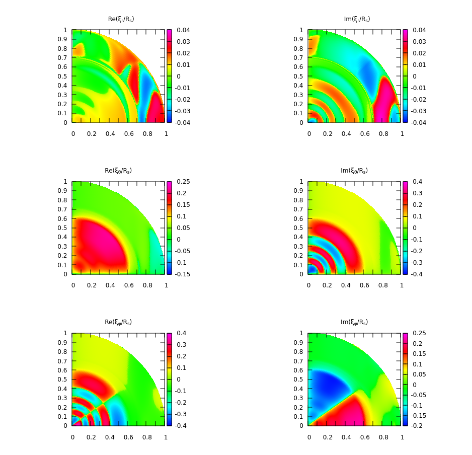
Figure 4: As in Fig. 3 but showing contour plots in the primary’s meridional plane $\phi=0$ for the resonant $l^{\prime}$=3 r mode with $n_{r}$ = 5 at resonance frequency $\omega_{0}=-3.332560283\times 10^{-3}$.

Figure 5: As in Fig. 3 but for contour plots in the primary’s meridional plane $\phi=0$ of the resonant $l^{\prime}$=5 r mode with $n_{r}$ = 0 at resonance frequency $\omega_{0}=-1.332426514\times 10^{-3}$.

Figure 6: As in Fig. 3 but for contour plots in the primary’s meridional plane $\phi=0$ of the resonant $l^{\prime}$=5 r mode with $n_{r}$ = 5 at resonance frequency $\omega_{0}=-1.332341064\times 10^{-3}$.

6.4 Convective envelope response

An $r$ mode sited in the radiative core excites a response in the convective envelope In appendix C we consider the response of the convective envelope in the limit of vanishing $|\omega_{f}|/(2\Omega_{s})$ .
This limit strictly applies only for very large $l^{\prime},$ though we find it of interest to make some comparison for $l^{\prime}=3,$ for which $|\omega_{f}|/(2\Omega_{s})\sim 1/6,$ and for $l^{\prime}=5,$ for which $|\omega_{f}|/(2\Omega_{s})\sim 1/15.$ In appendix C we find that in this limit $\xi_{\phi}$ should depend only on the cylindrical radius $\bar{r}.$ This tendency can be seen through the near vertical contour lines in Figs. 3 - 6 for all cases with $l^{\prime}=3$ and $l^{\prime}=5.$

In addition in the limit of vanishing $\omega_{f}$ we also find a critical latitude type singularity along the line $\bar{r}=r_{c}$ commencing at $z=0.$ However, we remark that in our case the Eckman number, $\nu/(2r_{c}^{2}\Omega_{s}),$ in this region is $\sim 10^{-4}$ which is significantly higher than those typically considered in inertial mode calculations (see eg. Rieutord & Valdetarro, 2010; Ogilvie, 2014). This would lead to an estimated thickness $\sim r_{c}(\nu/(2r_{c}^{2}\Omega_{s}))^{1/4}\sim 0.1r_{c}.$ Furthermore this scale is less than $r_{c}\sqrt{|\omega_{f}|/(2\Omega_{s})}\sim 0.2r_{c}$ for $l^{\prime}=5$ indicating that inertial waves play a part in the response (see discussion in Section C.1.2) which will be of quite a large scale. Nonetheless there is evidence of an incipient critical latitude phenomenon in $\xi_{r},$ particularly for $l^{\prime}=5$ ( see Figs. 3 - 6).

7 Effects on orbital and spin evolution

We now consider the effects of the tidal response of the primary on the orbital evolution of the system and the spin of the primary. As stated previously we here restrict consideration to aligned angular momenta and circular orbits.

7.1 Torque and dissipation resulting from tidal forcing

From (13) we see that the torque acting on $M_{p}$ is given by

$$M_{p}T_{Z}=-\left(\frac{4\pi GM_{p}}{5a^{3}}\right)(Y_{2,m}(\pi/2,0))mIm(Q_{m,\sigma})=-\frac{m}{\omega_{f}}\frac{dE_{kin}}{dt},$$ (39)

Note that for a positive dissipation rate, ${dE_{kin}}/{dt}=-dE_{dissip}/dt<0$ and by conservation of angular momentum the torque acting on the primary is, $T_{*}=-M_{p}T_{Z},$ accordingly we have

$$T_{*}=\frac{1}{\omega_{p}}\frac{dE_{dissip}}{dt},\hskip 8.53581pt{\rm where\hskip 2.84526ptthe\hskip 2.84526ptpattern\hskip 2.84526ptspeed\hskip 2.84526ptof\hskip 5.69054ptthe\hskip 2.84526ptforcing\hskip 5.69054pt}\omega_{p}=-\omega_{f}/m.$$

This leads to a putative rate of evolution of the orbit given by

$$\frac{M_{p}M_{*}}{2(M_{*}+M_{p})}\sqrt{\frac{G(M_{*}+M_{p})}{a}}\frac{da}{dt}=\frac{{\color[rgb]{0,0,0}|E_{orb}|}}{n_{0}}\frac{1}{a}\frac{da}{dt}=-\frac{1}{\omega_{p}}\frac{dE_{dissip}}{dt}.$$ (40)

with $E_{orb}$ being the orbital energy.

7.2 Orbital evolution

The torque acting on the primary results in evolution of its spin while its reaction causes evolution of the orbit. If only mutual gravitation and tidal forces act, the sum of the spin and orbital angular momentum is conserved. Thus we may write

$$J=|{\bf J}|=\mathcal{I}\,\Omega_{s}+\frac{M_{*}M_{p}}{(M_{*}+M_{p})}\sqrt{G(M_{*}+M_{p})a},$$ (41)

with $\mathcal{I}$ being the moment of inertia of the primary and, $J,$ the magnitude of the total angular momentum being constant (note that changes to, $J,$ induced by non tidal effects will be considered below). Assuming the system attains synchronisation, we set $\Omega_{s}=\sqrt{G(M_{*}+M_{p})/a^{3}}.$ Then we find

$$J(a)=\mathcal{I}\frac{\sqrt{G(M_{*}+M_{p})}}{a^{3/2}}+\frac{M_{*}M_{p}}{(M_{*}+M_{p})}\sqrt{G(M_{*}+M_{p})a},$$ (42)

From this one can see that, once, $J,$ is specified there are either two values, or no values, of $a$ for which the system is synchronised. For the former situation to apply we require

$$J>\frac{4}{3^{3/4}}\left(\frac{M_{*}M_{p}}{(M_{*}+M_{p})}\right)^{3/4}\sqrt{G(M_{*}+M_{p})}\,\mathcal{I}^{1/4}.$$ (43)

In that case the solution with the smaller value of $a$ is unstable. This means that for synchronisation, the semi-major axis must exceed the value one obtains when $J$ is specified to be the value given by (43) when the inequality is replaced by equality. This leads to

$$a\geq\left(\frac{3\,\mathcal{I}\,(M_{*}+M_{p})}{M_{*}M_{p}}\right)^{1/2}.$$ (44)

Expressing this in terms of the orbital period, $P_{orb},$ and a solar like primary, this gives

$$P_{orb}\geq 0.036\left(\frac{(1+q)^{1/4}}{q^{3/4}}\right)d.$$ (45)

For smaller periods in-spiral occurs with no approach to synchronisation especially when the star is slowly rotating. From the above it is clear that for a solar mass primary and $q\sim 1$ inequality (45) will in general be satisfied. On the other hand it is quite reasonable that it is not satisfied for $q\sim 0.001$ corresponding to secondaries in the giant planet mass regime and (45) turns out not to be satisfied for almost all objects classified as hot Jupiters. Thus these objects will not attain synchronisation under the above assumption of conservation of angular momentum given by Equation (42).

In this context we remark that the system for which we described the r mode resonances with $l^{\prime}=3$ in Section 6.2 has $a=1.61\times 10^{12}$ cm which exceeds the value given above ($1.04\times 10^{12}$ cm for a Jupiter mass planet) so allowing for the possibility of synchronisation. In addition $\Omega_{s}>n_{o}$ so that tidal effects will increase $a$, thereby slowing down the orbit while spinning down the primary more rapidly. This would move the system towards synchronisation. Only if the primary spins down (beyond synchronism) to the point where $\Omega_{s}<n_{0}$, for example due to magnetic braking, will tides lead to smaller $a$ values.

7.3 The effect of r mode resonances

The discussion in Section (7.2) is important when assessing the effects of normal mode resonances on the orbital evolution. The form of the $r$ modes that can be resonantly excited by tides is discussed in appendix B. For a given azimuthal mode number, $m,$ the resonant forcing frequencies seen in a frame co-rotating with the star are close to the values given by equation (34) ( see Section 6.1).

Recalling that when the total angular momentum of the system is conserved, if condition (45) is satisfied the spin and orbital periods approach each other more closely and the system moves towards synchronisation. In that case for a system with conserved total angular momentum the effect of encountering the resonances will be to cause the system to pass through brief periods of rapid tidal evolution moving the system towards synchronisation. On the other hand if condition (45) is not satisfied the system moves away from synchronisation undergoing periods of brief acceleration as the resonances are encountered. These processes occur in addition to effects due to the response of the convective envelope which may also be erratic.

7.4 Numerical calculation of spin and orbit evolution in the case of a Jupiter mass companion

The tidal evolution of the star/planet system caused by the viscous dissipation in the primary’s convective envelope is given by the following two equations where $\omega_{p}$ is the pattern speed of the considered $r$ mode

$$\mathcal{I}\,{{\mathrm{d}\Omega_{s}}\over{\mathrm{d}t}}=\frac{1}{\omega_{p}}\,{{\mathrm{d}E_{\rm{disp}}}\over{\mathrm{d}t}}$$ (46)

where $\mathcal{I}=6.851\times 10^{53}$ g cm${}^{2}=0.0782M_{*}R_{*}^{2},$ is the primary’s moment of inertia. The rate of change of the semi-major axis is (see section (7.1)

$${{\mathrm{d}a}\over{\mathrm{d}t}}=-\frac{2n_{o}}{\omega_{p}}\,\frac{a^{2}}{GM_{p}M_{*}}\,{{\mathrm{d}E_{\rm{disp}}}\over{\mathrm{d}t}}$$ (47)

where the viscous dissipation rate $dE_{\rm{disp}}(\omega_{f}-\omega_{0})/dt=-dE_{\rm{kin}}/dt$ follows from the fitted resonance curve for the considered r mode resonance, see tables 1 and 2. It is important to take into account that the resonance frequency $\omega_{0}$ of the r mode depends on the actual spin rate $\Omega_{s}$ of the primary during the tidal evolution of the system. To lowest order we simply assume that the resonance frequency $\omega_{0}$ scales linearly with $\Omega_{s}.$ Thus

$$\omega_{0}(t)=\omega_{0}(*)\,\frac{\Omega_{s}(t)}{\Omega_{s}(*)}$$ (48)

whereby $\omega_{0}(*)$ is the value given in table 1 and $\Omega_{s}(*)$ is the associated stellar angular velocity. The differential equations (46) - (47) are solved over time using a fifth order Runge-Kutta integration algorithm with adaptive step size control. As an example we calculated the passage through the strongest r mode resonance ($l^{\prime}=3$ with $n_{r}=0$ ) starting at $\omega_{f}-\omega_{0}=-1.0\times 10^{-8}$ up to $\omega_{f}-\omega_{0}\simeq+1.0\times 10^{-8}$.

Figure 7: The left panel shows the tidal evolution of the semi-major axis $a$ in units of $0.01\ au$ during resonance passage of the $l^{\prime}$=3 r mode with $n_{r}=0.$ The right hand panel shows the corresponding evolution of the primary’s angular velocity in units of $10^{-6}$ Hz.

Figure 8: The left panel shows the tidal evolution of the semi-major axis $a$ in units of $0.01\ au$ during resonance passage of the $l^{\prime}$=3 r mode with $n_{r}=0.$ Magnetic braking speeds up the tidal evolution. The right hand panel shows the corresponding evolution of the primary’s angular velocity in units of $10^{-6}$ Hz.

Figure 9: The left panel shows the tidal evolution of the semi-major axis $a$ in units of $0.01\ au$ during resonance passage of the $l^{\prime}$=5 r mode with $n_{r}=0.$ The right hand panel shows corresponding evolution of the primary’s angular velocity in units of $10^{-6}$ Hz. The unit of time is $10^{3}y.$

The results are displayed in Fig. 7. The orbit rapidly accelerates through the resonance with an average evolution timescale $a/\dot{a}\simeq 3\times 10^{7}$ y (from reaching 10 % of the full resonant dissipation rate left of the resonance up to the same rate on the right). This can be seen from applying equation (47) directly making use of the data plotted in Fig. 2, which leads to $a/\dot{a}\simeq 8\times 10^{7}$ y at. 10% of the full dissipation rate. However, as noted in section 6.2, nonlinear effects are likely to play a role during resonance passage and effectively cause an extension of this time scale. But we remark that initial and final forcing frequencies are far into the wings of the resonance (see Fig.2), where we might expect the linear approach to be valid.

Nevertheless, as noted in Section 6.2.1 we can expect the linear results to be valid for lower mass planets with masses $\sim 30$ times smaller, thus in the mini-Neptune range. Applying equation (47) at the centre of the resonance in this case yields $a/\dot{a}\simeq 2.4\times 10^{8}$ y indicating the potential significance of resonances in producing strong local torques. In corroboration of this, simple scaling of (47) indicates that $a/\dot{a}$ at the centre of the resonance is $\sim 30$ times smaller than it is for a Jupiter mass planet at the point where the energy dissipation rate is reduced by a factor $10^{3}.$

Returning to consideration of Jupiter mass planets, observations of G type dwarfs in star clusters (Skumanich, 1972; Smith, 1979) indicate that their rotational velocity on the Main Sequence decreases in time as $v_{eq}=A/\sqrt{t}$ cm/sec, where the proportionality factor $A$ is not accurately known. The stellar spin down is thought to be caused by magnetic braking due to the coupling between the stellar magnetic field and the outflowing stellar wind. To investigate its possible effect on the tidal evolution we use Skumanich’s result in the form

$${{\mathrm{d}\Omega_{s}}\over{\mathrm{d}t}}=-\frac{1}{2}\left(\frac{R_{*}}{A}\right)^{2}\,\Omega^{3}_{s}$$ (49)

and adopt $A=7.3\times 10^{13}$ cgs. The extra rate of magnetic down spinning is added to the right side of equation (46). Figure 8 shows the same $l^{\prime}=3$ with $n_{r}=0$ resonance passage as mentioned above but now including magnetic braking of the primary star. The system now moves faster into and out of full resonance due to the stronger spin down of the primary whereby in the outer wings of the resonance the magnetic braking contributes about $3/4$ of the total spin down. The time scale for stellar spin down at viscous dissipation rates of $10^{-3}$ and $2\times 10^{-3}$ of the full resonance value, taking into account both magnetic braking and tidal effects, is $\Omega_{s}/\dot{\Omega}_{s}\sim 10^{9}$ y and $\sim 7\times 10^{8}$ y, respectively, compared to $\sim 2.5\times 10^{9}$ y and $\sim 1.4\times 10^{9}$ y, respectively, without magnetic braking. Corresponding results for the orbital expansion timescale are $a/\dot{a}\simeq 7.7\times 10^{9}$ y and $\simeq 4\times 10^{9}$ y, respectively, without magnetic braking with only marginally smaller timescales when magnetic braking is included. By comparing these results with those in sections (7.5) and (7.5.1) the potential significance of resonances for tidal evolution for orbital periods up to $\sim 12$ d for Jupiter mass companions is evident under the condition that proximity to them can be maintained. As results are sensitive to the specification of the way the resonance frequency changes and the magnetic braking prescription it may be of interest to consider these processes using a more accurate expression for the changing resonance frequency obtained numerically during the tidal evolution.

7.4.1 Resonance passage when $l^{\prime}=5$

The strongest resonance with $l^{\prime}=5$ has $n_{r}=0$ as is the case for $l^{\prime}=3.$ As the $l^{\prime}=5$ resonance is weaker we we expect the resonance passage to be slower. Figure 9 shows the results of the calculation with $l^{\prime}=5$ corresponding to that with $l^{\prime}=3$ illustrated in in Figure 7. A comparison of these indicates the rate of evolution in the wings is slowed down by approximately one order of magnitude. This is mainly due to the resonance with $l^{\prime}=5$ being significantly narrower. However, evolution near the centre of resonance is still rapid, thus such a resonance may be significant for tidal evolution if it can be maintained.

7.5 Viscous dissipation rate for off-resonant tidal forcing

Up to now we have considered conditions in the neighbourhood of $r$ mode resonances and noted the possibility of significant tidal evolution. We now consider the tidal evolution expected out of resonance, in particular between the $l^{\prime}=3$ and $l^{\prime}=5$ r mode resonances considered above.

Figure 10 shows the viscous dissipation rate for forcing frequencies $\omega_{f}$ in between the $l^{\prime}=3$ and $l^{\prime}=5$ r mode resonances. The dissipation rate is seen to attain a minimum about half way between the resonances of around $5\times 10^{23}$ erg s${}^{-1}.$ The corresponding forcing frequency is
$\omega_{f}=-m\omega_{p}=-0.002\,\Omega_{c}.$ From equation (47) the time scale for evolution of the semi-major axis is related to this by

$$a\left(\frac{da}{dt}\right)^{-1}=-\left(\frac{dE_{dissip}}{dt}\right)^{-1}\frac{\omega_{p}|E_{orb}|}{n_{o}}$$ (50)

From (50) we find that $a/\dot{a}=1.25\times 10^{12}\,y$ for an orbital period of $13.4\,d.$ Thus we find, as expected, that the global tidal evolution significantly exceeds the life time of the system. The time to move between the $l^{\prime}=3$ and $l^{\prime}=5$ resonances at $\sim 4\times 10^{10}y$ is still long compared to the expected age but approaching becoming marginal.

In contrast to the situation off resonance, from the results given in tables 1 and 2 we find that r mode resonances tidally excited in the radiative core of the primary can lead to rapid tidal evolution. However, the large dissipation rate drives the system quickly through the resonance so that the global effects are limited unless mechanisms act to maintain the system close to resonance (see below).

Figure 10: The upper panel shows the viscous dissipation rate (erg/s) with $\omega_{f}$ in the frequency range between the $l^{\prime}=3$ and $l^{\prime}=5$ r mode resonances, being inside the inertial range. The lower panel shows the viscous dissipation rate (erg/s) for tidal forcing with frequencies $\omega_{f}$ outside the inertial range. The forcing frequency, here $>0,$ varies between $3.5$ and $4.5$ times the rotation frequency, the limit of the inertial range being twice the rotation frequency.

7.5.1 Viscous dissipation rate for tidal forcing outside the inertial range

The off resonant dissipation considered above occurs in the inertial regime such that inertial modes can be excited in the convective envelope. Here we consider the situation where this does not apply. Figure 10 shows the viscous dissipation rate for forcing frequencies $|\omega_{f}|>2\,\Omega_{s}$ outside the inertial range. The now chosen positive forcing frequency varies from $3.5$ to $4.5$ times the rotation frequency and the viscous dissipation rate varies from $\simeq 1.5\times 10^{23}$ at orbital period 3.91 d, to $3\times 10^{23}$ ergs^-1 at orbital period 3.31 d. With $m=-2$ the forcing is now prograde. In this frequency range there is some contribution to the tidal response by high radial order ($n\simeq 100$) $g$ modes which were damped through the numerical procedure near the stellar centre where their wavelength becomes shorter than the grid spacing. From equation (50) we find that the viscous dissipation in the stellar envelope corresponds to an orbital decay rate $a/\dot{a}=-2.3\times 10^{13}$ y for $\omega_{f}=3.5\times 10^{-2}$ and $-1.4\times 10^{13}$ y for $\omega_{f}=4.5\times 10^{-2}$, again implying that evolution in this regime will be negligible. It is of interest to compare this with the prediction of equation (6.1) of Zahn (1977). According to this for tides exerted on a solar mass star by a Jupiter mass planet with an orbital period of 3.31 d the synchronisation time is $3\times 10^{11}y$ which, although also predicting negligible evolution, is shorter by a factor of $50.$ However, equation (6.1) of Zahn (1977) does not include the expected but very uncertain reduction in turbulent viscosity resulting from a mismatch between convective and orbital time scales, see equation (21). This is significant for these short orbital periods and accounts for the discrepancy.

7.6 The possibility of evolution with resonant interaction maintained

For the $r$ mode resonances to be maintained as the system evolves some parameters defining the system such as the total angular momentum, the masses of the components, and/or the moment of inertia of the primary have to be envisaged to change. Here for simplicity we shall only consider variation of the total angular momentum. Suppose that resonance is maintained with the mode with $l^{\prime}=3,|m|=2$ with frequency $\omega_{p}=-\Omega_{s}/6$ and hence $\Omega_{s}=6n_{0}/5.$ Using this condition rather than $\Omega_{s}=n_{o}$ the expression for the total angular momentum, $J,$ given by (42) becomes

$$J(a)=\frac{6\,\mathcal{I}}{5}\frac{\sqrt{G(M_{*}+M_{p})}}{a^{3/2}}+\frac{M_{*}M_{p}}{(M_{*}+M_{p})}\sqrt{G(M_{*}+M_{p})a}$$ (51)

This has a minimum when, $a=a_{min},$ given by

$$a_{min}=\left(\frac{18\,\mathcal{I}(M_{*}+M_{p})}{5M_{*}M_{p}}\right)^{1/2}.$$ (52)

For a solar mass primary this corresponds to an orbital period, $P_{orb,min},$ where

$$P_{orb,min}=0.045\left(\frac{\mathcal{I}}{0.0782M_{*}R_{*}^{2}}\right)^{3/4}\frac{(1+q)^{1/4}}{q^{3/4}}\left(\frac{M_{\odot}}{M_{*}}\right)^{1/2}\left(\frac{R_{*}}{R_{\odot}}\right)^{3/2}d$$ (53)

When, $a>a_{min},$ evolution maintaining resonance requires, $a,$ to increase while the primary spins down. Equation (51) then indicates that, with other parameters fixed, the magnitude of the total angular momentum, $J,$ increases. Accordingly this kind of evolution requires angular momentum transfer to the system. But note as indicated above that changes of other parameters could have the same effect.

On the other hand when $a<a_{min},$ evolution maintaining resonance also requires, $a,$ to increase while the primary spins down. In this case Equation (51) indicates that, with other parameters fixed, the magnitude of the total angular momentum, $J,$ decreases. Some mechanism for bringing this about such as the effect of a stellar wind needs to be invoked. Note that in this case $a$ cannot increase beyond $a_{min}.$ As noted above the case $a<a_{min}$ applies to almost all hot Jupiters making this form of evolution a possibility at some phase of their lifetime. However, we note that the condition of being close to synchronisation requires a rapidly rotating primary, a possibility that may not be realised. In addition the ability to maintain a state of uniform rotation has to be assumed.

8 Discussion

In this paper we have calculated the tidal response of a rotating solar type primary to the tidal forcing of a planetary mass companion. Although rotation is considered small in the sense that Coriolis forces are retained with centrifugal forces being neglected, we do not make the traditional approximation which is not valid in convective regions. Tidal forcing frequencies as seen in the frame corotating with the primary that are smaller in magnitude than $2\Omega_{s}$, and so are in the inertial regime, are considered (Papaloizou & Pringle, 1981; Ogilvie & Lin, 2007). For a first set of detailed calculations, we limited consideration to a circular orbit in the period range of $10-14d,$ leaving extensions to future work.

With a view to application to exoplanets we focused on a Jupiter mass companion though results can be scaled to apply to companions of arbitrary mass. Resonantly excited modes of oscillation can be important for tidal evolution (see e.g. Savonije & Papaloizou, 1983; Witte & Savonije, 2002; Zanazzi & Wu, 2021). Hence we focused on identifying and calculating the resonant response associated with $r$ modes (Papaloizou & Pringle, 1978) which are predominantly sited in the radiative core. We gave the properties of this spectrum of modes for $l^{\prime}=3$ and $l^{\prime}=5$ obtained numerically in Section 6.2 with a semi-analytic treatment in appendix B. We described the response of the convective envelope, where most of the dissipation occurs through the action of turbulent viscosity in Section 6.4. A semi-analytic discussion applicable in the low tidal forcing frequency limit is given in appendix C which relates to the behaviour of the horizontal displacements and an incipient critical latitude phenomenon.

We formulated the effects of the tidal response on the orbital and spin evolution of the system in Sections 7 - 7.2. The effect of r mode resonances is to greatly speed up the orbital evolution over a narrow frequency range in their vicinity and their effect on orbital evolution is limited if the primary’s structure is fixed and the total angular momentum is conserved.

We described the results of numerical calculations of spin and orbit evolution in Section 7.4. Non resonant tidal forcing between the $l^{\prime}=3$ and $l^{\prime}=5$ resonances which lies within in the inertial regime gives rise to orbital evolution times $\sim 10^{12}y$ which greatly exceeds potential system lifetimes. However, the evolution time between the $l^{\prime}=3$ and $l^{\prime}=5$ resonances with are separated by only $\delta a\sim 0.07a$ approaches this to within an order of magnitude for orbital periods $\sim 13.4d.$

Non-resonant tidal forcing at higher frequencies lying outside the inertial regime is even slower occuring on a time scale $\sim 2\times 10^{13}y$ ( see Sections 7.5 and 7.5.1). As rotation is expected to have a small effect in this regime, with making allowance for reductions in turbulent viscosity due to frequency mispatch, the result was found to be consistent with the results of Zahn (1977) for a non rotating star.

Significant orbital evolution over a realistic lifetime of the system can only be found if resonant interaction that provides enhanced tidal interaction is maintained. Such resonance locking has been invoked as a method of speeding up tidal evolution in a number of astrophysical contexts including binary star and exoplanet systems (see Ma &Fuller, 2021; Zanazzi & Wu, 2021). For a discussion of the process of resonance locking see e.g. Fuller et al. (2016). Resonance locking either requires a substantial orbital eccentricity (Witte & Savonije, 1999) or parameters defining the system which could be the total angular momentum or the stellar moment of inertia to change.

Such changes could be produced by well established phenomena such as magnetic braking in the former case or the effects of stellar evolution in the latter. For systems such as hot or warm Jupiters it was found that significant evolution within the system lifetime could occur at a separation from the resonance centre where the dissipation rate was $1000$ times smaller than at the peak and the linear response plausibly applicable. For these systems there is the possibility of sustained tidal evolution with increasing orbital period and maintained proximity to resonance driven by angular momentum loss due to a stellar wind at some phase of their lifetime (Section 7.6), provided the primary spins rapidly enough initially and the orbital period is. such that

$$P_{orb}<P_{orb,min}=0.045\left(\frac{\mathcal{I}}{0.0782M_{*}R_{*}^{2}}\right)^{3/4}\frac{(1+q)^{1/4}}{q^{3/4}}\left(\frac{M_{\odot}}{M_{*}}\right)^{1/2}\left(\frac{R_{*}}{R_{\odot}}\right)^{3/2}d.$$ (54)

The extent of this is dependent on the angular momentum loss mechanism (see Section 7.6). When the inequality in (54) reversed resonance locked evolution requires the orbital period and the system angular momentum to increase with time as could possibly be driven by mass accretion.

Processes of the type described above are expected to be effective only when resonance locking is sustained on account of evolutionary changes to the system such as angular momentum loss through a wind, and the central star is rapidly rotating. Systems in which they are currently operating are likely to be young with the central stars possessing a significant radiative core.

In addition an expected observational signature should be that the stellar rotation period is shorter than the orbital period and satisfies $(5P_{rorb})/6\leq P_{rot}\leq P_{orb},$ allowing a resonance condition to be satisfied. Then the system loses/gains angular momentum according to whether the inequality (54) is satisfied/not satisfied.

A tentative candidate system is Kepler 1643 (see Bouma et al., 2022). This has $M_{*}=0.92M_{\odot}$, $R_{*}=0.88R_{\odot},$ with a rotation period $P_{rot}=5.106d,$ and an estimated age $\sim 4\times 10^{7}y.$ The orbital period is $5.3426d.$ The mass of the planet described as a mini-Neptune is uncertain, accordingly for illustrative purposes we adopt the characteristic value $M_{p}=M_{J}/30.$ The condition,
$(5P_{rorb})/6\leq P_{rot}\leq P_{orb},$ is satisfied with the expected resonance for $l^{\prime}=5,$ and $n_{r}=0$ being close to $P_{rot}=4.99d.$ Noting theoretical and observational uncertainties arising from effects such as the relation of surface to interior rotation, this is in reasonable agreement with the quoted value. In this case the inequality (54), evaluated here and below assuming the first term in brackets on the right hand side is unity, indicates the system should be losing angular momentum possibly due to a stellar wind.

Another system in which tidal evolution with resonance locking may have occurred is
COROT - 4 (see Moutou et al., 2008). This has $P_{orb}=9.20d,$ $M_{p}=0.72M_{J}$ with $M_{*}=1.16M_{\odot},$ $R_{*}=1,17R_{\odot}.$ and $P_{rot}=8.87\pm 1.12d.$ With an estimated age $\sim 1Gy,$ angular momentum loss through a wind may have slowed significantly. The inequality (54) is satisfied with $P_{orb}<13.44d$ so the resonance condition should be maintained. The $l^{\prime}=3$ resonance is near $P_{rot}=5/6P_{orb}=7.67d,$ and the $l^{\prime}=5$ resonance is near to $P_{rot}=14P_{orb}/15=8.59d$ both of which could be possible in view of the uncertainties. In particular resonance locking may explain why this system has been able to attain a near synchronous state at its relatively long orbital period.

In this paper we have concentrated on aligned systems in circular orbits over a limited period range. The effects of resonant $r$ mode excitation found here should be more pronounced at shorter periods making a detailed survey is of interest. In addition, the extension to misaligned systems is important in the context of the possibility of tidal alignment of hot Jupiter orbits, in particular whether this happens more rapidly than tides acting in aligned systems can operate. The existence of $r$ modes with $l^{\prime}=|m|=1$ is promising as these may always be close to resonance. These aspects will be the subject of future work.

9 Data Availability

The data underlying this article will be shared on reasonable request to the corresponding author.

Appendix A The components of the viscous stress tensor

Recalling that it is symmetric, the components of the viscous stress tensor, $\mbox{\boldmath$\mathsf{\Sigma}$},$ expressed in spherical coordinates in terms of the components of the associated displacement vector, $\mbox{{\boldmath$\xi$}},$ are given by

$$\mbox{\boldmath$\mathsf{\Sigma}$}_{rr}=2\rm i\,\omega_{f}\,\rho\nu\left[\frac{\partial\xi_{r}}{\partial r}-\frac{1}{3}\nabla\cdot\mbox{{\boldmath$\xi$}}\right]$$

$$\mbox{\boldmath$\mathsf{\Sigma}$}_{\theta,\theta}=2\rm i\,\omega_{f}\,\rho\nu\left[\left(\frac{1}{r}\frac{\partial\xi_{\theta}}{\partial\theta}+\frac{\xi_{r}}{r}\right)-\frac{1}{3}\nabla\cdot\mbox{{\boldmath$\xi$}}\right]$$

$$\mbox{\boldmath$\mathsf{\Sigma}$}_{\varphi,\varphi}=2\rm i\,\omega_{f}\,\rho\nu\left[\frac{1}{r\,\sin\theta}\frac{\partial\xi_{\varphi}}{\partial\varphi}+\frac{\xi_{r}}{r}+\frac{\xi_{\theta}}{r\,\tan\theta}-\frac{1}{3}\nabla\cdot\mbox{{\boldmath$\xi$}}\right]$$

$$\mbox{\boldmath$\mathsf{\Sigma}$}_{r\theta}=\rm i\,\omega_{f}\,\rho\nu\left[\frac{\partial\xi_{\theta}}{\partial r}+\frac{1}{r}\frac{\partial\xi_{r}}{\partial\theta}-\frac{\xi_{\theta}}{r}\right]$$

$$\mbox{\boldmath$\mathsf{\Sigma}$}_{\theta\varphi}=\rm i\,\omega_{f}\,\rho\nu\left[\frac{1}{r\,\sin\theta}\frac{\partial\xi_{\theta}}{\partial\varphi}+\frac{1}{r}\frac{\partial\xi_{\varphi}}{\partial\theta}-\frac{\xi_{\varphi}}{r\,\tan\theta}\right]$$

$$\mbox{\boldmath$\mathsf{\Sigma}$}_{\varphi r}=\rm i\,\omega_{f}\,\rho\nu\left[\frac{\partial\xi_{\varphi}}{\partial r}+\frac{1}{r\sin\theta}\frac{\partial\xi_{r}}{\partial\varphi}-\frac{\xi_{\varphi}}{r}\right]$$

A.1 The divergence of the tensor, $\mbox{\boldmath$\mathsf{\Sigma}$}.$ in spherical coordinates

The divergence of $\mathsf{\Sigma}$ is required to evaluate the viscous force per unit mass associated with the displacement ${\xi}$ indicated above. This is given by

$$\nabla\cdot\mbox{\boldmath$\mathsf{\Sigma}$}= \left(\frac{1}{r^{2}}\frac{\partial}{\partial r}(r^{2}\mbox{\boldmath$\mathsf{\Sigma}$}_{r,r})+\frac{1}{r\sin\theta}\frac{\partial}{\partial\theta}(\sin\theta\mbox{\boldmath$\mathsf{\Sigma}$}_{r,\theta})+\frac{1}{r\sin\theta}\frac{\partial}{\partial\phi}(\mbox{\boldmath$\mathsf{\Sigma}$}_{r,\phi})-\frac{(\mbox{\boldmath$\mathsf{\Sigma}$}_{\theta,\theta}+\mbox{\boldmath$\mathsf{\Sigma}$}_{\phi,\phi})}{r}\right){\hat{\bf r}}$$

$$+\left(\frac{1}{r^{2}}\frac{\partial}{\partial r}(r^{2}\mbox{\boldmath$\mathsf{\Sigma}$}_{r,\theta})+\frac{1}{r\sin\theta}\frac{\partial}{\partial\theta}(\sin\theta\mbox{\boldmath$\mathsf{\Sigma}$}_{\theta,\theta})+\frac{1}{r\sin\theta}\frac{\partial}{\partial\phi}(\mbox{\boldmath$\mathsf{\Sigma}$}_{\theta,\phi})+\frac{(\mbox{\boldmath$\mathsf{\Sigma}$}_{r,\theta}-\mbox{\boldmath$\mathsf{\Sigma}$}_{\phi,\phi}\cot\theta)}{r}\right){\hat{\bf\mbox{\boldmath$\theta$}}}$$

$$+\left(\frac{1}{r^{2}}\frac{\partial}{\partial r}(r^{2}\mbox{\boldmath$\mathsf{\Sigma}$}_{r,\phi})+\frac{1}{r\sin\theta}\frac{\partial}{\partial\theta}(\sin\theta\mbox{\boldmath$\mathsf{\Sigma}$}_{\phi,\theta})+\frac{1}{r\sin\theta}\frac{\partial}{\partial\phi}(\mbox{\boldmath$\mathsf{\Sigma}$}_{\phi,\phi})+\frac{(\mbox{\boldmath$\mathsf{\Sigma}$}_{r,\phi}+\mbox{\boldmath$\mathsf{\Sigma}$}_{\theta,\phi}\cot\theta)}{r}\right){\hat{\bf\mbox{\boldmath$\phi$}}}$$

where, ${\bf\mbox{\boldmath$r$}},{\bf\mbox{\boldmath$\theta$}},{\bf\mbox{\boldmath$\phi$}}$, respectively denote unit vectors in the, $(r,\theta,\phi),$ directions

Appendix B The r mode spectrum in radiative regions in the low frequency adiabatic limit

We begin by formulating the basic equations governing the tidal response and then proceed to consider their solution in the limit that the forcing frequency as seen in the rotating frame is small while being comparable in magnitude to the rotation frequency while adopting the Cowling approximation in which response perturbations to the gravitational potential are neglected.

B.1 Linearised equation of motion

The linearised equation of motion governing the tidal response given by equation (15) in the limit that perturbations are assumed to be adiabatic ( the RHS of equation (17) set to zero ) under the Cowling approximation in which perturbation to the gravitational potential is neglected is

$$-{\omega_{f}}^{2}{\mbox{\boldmath$\xi$}}+2{\rm i}{\omega_{f}}{\mbox{\boldmath$\Omega_{s}$}\times}{\mbox{\boldmath$\xi$}}=-\frac{F}{\rho}\nabla W-N^{2}\left(\xi_{r}+\frac{U}{g}\right){\bf{\hat{r}}}$$ (55)

Here for ease of notation the subscripts, $m,$ and $\sigma,$ have been dropped from the forcing potential ${U},$ ${\mbox{\boldmath$\xi$}}\equiv(\xi_{r},\xi_{\theta},\xi_{\phi})$ and other perturbations and will be taken as read in this and subsequent appendices. The quantity $W=(P^{\prime}+\rho U)/F,$ with $d\ln F/dr=(d\ln P/dr)/\Gamma_{1},$
The square of the buoyancy frequency is $N^{2}=g(1/(\Gamma_{1}P)dP/dr-(1/\rho)d\rho/dr),$ $g$ is the acceleration due to gravity, and the adiabatic exponent $\Gamma_{1}=(\rho/P)d\ln P/d\ln\rho.$ We recall that ${\omega_{f}}=\sigma+m\Omega_{s}$ is the forcing frequency as seen in the rotating frame. We remark that the quantity $\xi_{r,eq}=-U/g$ is the standard equilibrium tide.

The components of the linearised equation of motion in spherical polar coordinates are

$$-{\omega_{f}}^{2}\xi_{r}-2{\rm i}{\omega_{f}}\Omega_{s}\sin\theta\xi_{\phi}=-\frac{F}{\rho}\frac{\partial W}{\partial r}-N^{2}\left(\xi_{r}+\frac{U}{g}\right)$$ (56)

$$-{\omega_{f}}^{2}\xi_{\theta}-2{\rm i}{\omega_{f}}\Omega_{s}\cos\theta\xi_{\phi}=-\frac{F}{\rho r}\frac{\partial W}{\partial\theta}$$ (57)

$$-{\omega_{f}}^{2}\xi_{\phi}+2{\rm i}{\omega_{f}}\Omega_{s}(\sin\theta\xi_{r}+\cos\theta\xi_{\theta})=-\frac{{\rm i}mWF}{\rho r\sin\theta}$$ (58)

B.1.1 Decomposition into spheroidal and toroidal components

We write the radial displacement as the sum of equilibrium tide value and a correction $\eta_{r},$ and without loss of generality write the horizontal displacement as the sum of spheroidal and toroidal contributions. Thus

$$\xi_{r}=\xi_{r,eq}+\eta_{r}$$ (59)

$$\xi_{\theta}=\frac{1}{r\sin\theta}\frac{\partial{\cal T}}{\partial\phi}+\frac{1}{r}\frac{\partial S}{\partial\theta}\equiv\frac{{\rm i}m}{r\sin\theta}{\cal T}+\frac{1}{r}\frac{\partial S}{\partial\theta}$$ (60)

$$\xi_{\phi}=-\frac{1}{r}\frac{\partial{\cal T}}{\partial\theta}+\frac{1}{r\sin\theta}\frac{\partial S}{\partial\phi}\equiv-\frac{1}{r}\frac{\partial{\cal T}}{\partial\theta}+\frac{{\rm i}m}{r\sin\theta}S$$ (61)

Making use of (60) and (61) we may eliminate $\xi_{\theta}$ and $\xi_{\phi}$ in (57) and (58) in favour of $S$ and ${\cal T}$ and then eliminate $W.$ This leads to the equation

$$\frac{{\omega_{f}}^{2}}{r^{2}}\nabla^{2}_{\perp}{\cal T}+\frac{2m\Omega_{s}{\omega_{f}}}{r^{2}}{\cal T}+\frac{2{\rm i}{\omega_{f}}\Omega_{s}\cos\theta}{r^{2}}\nabla^{2}_{\perp}S-\frac{2{\rm i}\Omega_{s}{\omega_{f}}\sin\theta}{r^{2}}\frac{\partial S}{\partial\theta}=-\frac{2{\rm i}{\omega_{f}}\Omega_{s}}{r\sin\theta}\frac{\partial(\sin^{2}\theta\xi_{r})}{\partial\theta}.$$ (62)

which relates ${\cal T}$ to $S$ and $\xi_{r}.$ Here $\nabla^{2}_{\perp}{\cal Q}$ for some quantity ${\cal Q}$ is defined through

$$\nabla_{\perp}^{2}{\cal Q}=\frac{1}{\sin\theta}\frac{\partial}{\partial\theta}\left(\sin\theta\frac{\partial{\cal Q}}{\partial\theta}\right)-\frac{m^{2}{\cal Q}}{\sin^{2}\theta}$$

In addition we may make use of (60) and (61) to find an expression for $F/(\rho r)\nabla^{2}_{\perp}W$ which is thus found to be given by

$$\frac{F}{\rho r}\nabla^{2}_{\perp}W=\frac{\omega^{2}_{f}}{r}\nabla^{2}_{\perp}S-2\Omega\omega_{f}{\rm i}\left(\frac{\mu}{r}\nabla^{2}_{\perp}{\cal T}+\frac{(1-\mu^{2})}{r}\frac{\partial{\cal T}}{\partial\mu}+\frac{\partial}{\partial\phi}\left(\xi_{r}+\frac{S}{r}\right)\right).$$ (63)

Using this together with (56) enables a second relation between $\xi_{r},$ $S,$ and ${\cal T}.$ To complete the system we need to make use of the continuity equation and adiabatic condition.

B.2 Linearised continuity equation and adiabatic condition

The linearised continuity equation is

$$\rho^{\prime}=-\nabla\cdot(\rho{\mbox{\boldmath$\xi$}})$$ (64)

and the adiabatic condition is

$$P^{\prime}=WF-\rho U=-\frac{\Gamma_{1}P}{F}\nabla\cdot(F{\mbox{\boldmath$\xi$}})$$ (65)

Making use of (60) and (61) equation (65) may be written as

$$WF-\rho U=\frac{\Gamma_{1}P}{r^{2}}\left(\frac{1}{F}\frac{\partial(r^{2}FUg^{-1})}{\partial r}-\frac{1}{F}\frac{\partial(r^{2}F\eta_{r})}{\partial r}-\nabla_{\perp}^{2}S\right).$$ (66)

B.3 The tidal response in the radiative zone in the limit of small forcing and rotation frequencies

In this region in the limit, ${\omega_{f}}\rightarrow 0,$ given that, $N^{2}>0,$ remains finite, equation (56) implies that
$\eta_{r}\rightarrow 0,$ and so this can be regarded as small in comparison to the horizontal components of the displacement. Inspections of equations(57) and (58) indicates that the the contribution of. $WF,$ in comparison to the terms involving horizontal displacements in (65) is of order $r^{2}\rho\omega_{f}^{2}/(\Gamma_{1}P)$ as ${\omega_{f}}\rightarrow 0,$ This suggests we can neglect $W$ in that equation in that limit corresponding to an anelastic approximation.

We remark that in order to then proceed with (66) while retaining $\eta_{r}$ there when this quantity varies on a global length scale, we formally require a hierarchical ordering $\omega_{f}^{2}\ll N^{2}\ll\Gamma_{1}P/(\rho r^{2}).$ However, excessive values of $N^{2}$ can be compensated for by considering $\eta_{r}$ that vary on small scales.

B.4 Determination of $S$ and ${\cal T}$ in the limit of low forcing and rotation frequencies

After making the anelastic approximation we write

$$S=S_{1}+S_{2},\hskip 8.53581pt{\rm where}$$ (67)

$$r^{2}\rho{U}=\Gamma_{1}P\left(-\frac{1}{F}\frac{\partial(r^{2}F{U}g^{-1})}{\partial r}+\nabla_{\perp}^{2}S_{1}\right).$$ (68)

Equation (66) then implies that in the anelastic limit

$$\nabla_{\perp}^{2}S_{2}=-\frac{1}{F}\frac{\partial(r^{2}F\eta_{r})}{\partial r}.$$ (69)

Corresponding to (67) we write ${\cal T}={\cal T}_{1}+{\cal T}_{2},$ and $W=W_{1}+W_{2}.$ Equations for $S_{i},{\cal T}_{i},W_{i},$ can be obtained from equations (62) and (63) through the replacements $S\rightarrow S_{i},{\cal T}\rightarrow{\cal T}_{i},W\rightarrow W_{i},$ with $\xi_{r}\rightarrow\xi_{r,eq}$ for $i=1$ and $\xi_{r}\rightarrow\eta_{r}$ for $i=2.$ The corresponding horizontal displacement components are $(\xi_{\theta,i},\xi_{\phi,i}).$ Following the traditional approximation in the low forcing frequency and rotation limit, we shall subsequently neglect $\eta_{r}$ in (62) and (63) but importantly not in (69). We. remark that if $\eta_{r}$ were to be neglected in (69) as well and thus throughout, then ${\cal T}_{2}=S_{2}=W_{2}=0.$

B.4.1 Successive approximation

The above scheme results in ${\cal T}_{1}$ and $S_{1}$ being determined by the equilibrium tide (which we call the lowest order approximation) and $\eta_{r}$ being subsequently determined as a correction in the manner described below. Before doing this we remark that the $\eta_{r}$ so determined can be used to determine an approximation to, ${\cal T}_{2}$ and $W_{2}$ from the appropriate forms of equations (62) and (63). For tidal forcing $\propto Y_{l,m}(\theta,\phi),$ ${\cal T}_{1}$ (with $\eta_{r}$ neglected) will be found to involve spherical harmonics of degrees $l\pm 1$ (providing of course that in the case of the smaller alternative, $l-1\geq|m|$). We can then see from the appropriate form of equation (63) that $W_{1}$ will involve spherical harmonics of degrees $l\pm 2.$ Equation (56) then indicates that these values of $l$ will appear in an expansion of $\eta_{r}$ in spherical harmonics. These in turn will generate an additional component of degree $l+3$ in the expansion of ${\cal T}_{2}$ that is potentially resonant. Proceeding with successive approximations we see that we can expect toroidal mode resonances with all possible values of $l$ with the opposite parity to that of the original forcing potential. Having noted this we now focus on the simplest cases with degrees $l\pm 1$ as these can be studied at the lowest order of approximation

B.5 Determination of the toroidal mode response assuming the equilibrium tide for radial motions

Here we now determine $S_{1}$ and ${\cal T}_{1}$ in the lowest order approximation as indicated above.

B.5.1 Calculation of $S_{1}$

As $U$ is known equation (68) can be used to determine $S_{1}.$ For the case of interest, for which $U=r^{l}Y_{l,m}(\theta,\phi)\exp({\rm i}{{\omega_{f}}}t),$ we obtain

$$S_{1}={\cal S}_{1}Y_{l,m}(\theta,\phi)\exp({\rm i}{{\omega_{f}}}t),\hskip 8.53581pt{\rm where}$$ (70)

$$r^{l+2}\rho=-\Gamma_{1}P\left(\frac{1}{F}\frac{\partial(r^{l+2}Fg^{-1})}{\partial r}+l(l+1){\cal S}_{1}\right).$$ (71)

Making use of hydrostatic equilibrium this may be reduced to the simple expression

$${\cal S}_{1}=-\frac{1}{l(l+1)}\frac{d(r^{l+2}g^{-1})}{dr}.$$ (72)

B.5.2 Calculation of ${\cal T}_{1}.$

We now proceed to the determination of ${\cal T}_{1}$ from the adapted form of equation (62). this may be written in the form

$$\frac{{\omega_{f}}^{2}}{r^{2}}\nabla^{2}_{\perp}{\cal T}_{1}+\frac{2m\Omega_{s}{\omega}_{f}}{r^{2}}{\cal T}_{1}=R_{T},\hskip 8.53581pt{\rm where}$$ (73)

$$R_{T}=-\frac{2{\rm i}{\omega}_{f}\Omega_{s}\cos\theta}{r^{2}}\nabla^{2}_{\perp}S_{1}+\frac{2{\rm i}\Omega_{s}{\omega}_{f}\sin\theta}{r^{2}}\frac{\partial S_{1}}{\partial\theta}-\frac{2{\rm i}{\omega_{f}}\Omega_{s}r^{l-1}}{g}\frac{\partial((1-\mu^{2})Y_{l,m})}{\partial\mu}.$$ (74)

Making use of (70) and (68) we find

$$R_{T}\exp(-{\rm i}{\omega}t)=-{2{\rm i}{\omega_{f}}\Omega_{s}}\frac{d(r^{l}g^{-1})}{dr}\mu Y_{l,m}+2{\rm i}\Omega_{s}{\omega_{f}}\left(\frac{1}{l(l+1)r^{2}}\frac{d(r^{l+2}g^{-1})}{dr}-\frac{r^{l-1}}{g}\right)(1-\mu^{2})\frac{\partial Y_{l,m}}{\partial\mu}.$$ (75)

We solve (73) by writing ${\cal T}_{1}$ as a generic sum over spherical harmonics. Thus

$${\cal T}_{1}=r^{2}\exp({\rm i}{{\omega_{f}}}t)\sum_{l^{\prime}=|m|}^{\infty}{\cal D}_{l^{\prime}}(r)Y_{l^{\prime},m}(\theta,\phi),\hskip 8.53581pt{\rm where}$$ (76)

the coefficients ${\cal D}_{l^{\prime}}$ are determined by solving (73). By inspection of of (75) and making use of well known properties of spherical harmonics (see Abramowitz & Stegun, 1964) we find that for a given, $l,$ only the terms with $l^{\prime}=l-1$ and $l^{\prime}=l+1$ are non zero. In particular the non vanishing expansion coefficients are given by

$${\cal D}_{l-1}=\frac{{2{\rm i}\Omega_{s}}}{\omega_{f}l^{2}\left(1-2m\Omega_{s}/(\omega_{f}l(l-1))\right)}\left(r^{l}dg^{-1}/dr+2(l+1)r^{l-1}/g\right)\beta_{l,m}\hskip 8.53581pt{\rm and}$$ (77)

$${\cal D}_{l+1}=\frac{{2{\rm i}\Omega_{s}}}{\omega_{f}(l+1)^{2}\left(1-2m\Omega_{s}/(\omega_{f}(l+1)(l+2))\right)}\left(r^{l}dg^{-1}/dr+r^{l-1}/g\right)\alpha_{l,m},\hskip 5.69054pt{\rm where}$$ (78)

$$\alpha_{l,m}=\sqrt{\frac{(l-m+1)(l+m+1)}{(2l+1)(2l+3)}}\hskip 5.69054pt{\rm and}\hskip 5.69054pt\beta_{l,m}=\sqrt{\frac{(l-m)(l+m)}{(2l-1)(2l+1)}}$$ (79)

Note the potentially vanishing denominators at the $r$ mode resonances where ${\omega_{f}}=2m\Omega/(l^{\prime}(l^{\prime}+1).$ In our tidal problem with, $l=2,$ if $|m|=1,$ the resonances occur for $l^{\prime}=l-1=1$ and $l^{\prime}=l+1=3.$ For $|m|=2,$ from (76), only the case $l^{\prime}=3$ is present.

The coefficients ${\cal D}_{l-1}$ and ${\cal D}_{l+1}$ enable ${\cal T}_{1}$ to be found from (76) and the contribution this makes to the horizontal components of the displacement can then be found from (60) and (61) with the substitution ${\cal T}\rightarrow{\cal T}_{1}.$ Significantly ${\cal T}_{1}$ is affected by $r$ mode resonances but $S_{1}$ is not. Accordingly if we are close to resonance $S_{1}$ may be neglected.

As we shall focus on conditions close to resonance and accordingly terms potentially affected by resonant denominators, we remark that an expression for $W_{1}$ that contains these is most easily found from (58) on setting $W=W_{1},$ $\xi_{r}=0,$ while including only the contributions involving ${\cal T}_{1}$ on the left hand side, when that is expressed as a sum of spheroidal and toroidal components, as only this is amplified by resonance. This gives

$$\frac{W_{1}F}{\rho}=-\frac{{\rm i}\omega_{f}^{2}}{m}\left((1-\mu^{2})\frac{\partial{\cal T}_{1}}{\partial\mu}+\frac{2\Omega_{s}m\mu}{\omega_{f}}{\cal T}_{1}\right).$$ (80)

B.6 The effect of radial motions

The above analysis results, at lowest order, in singularities at single toroidal mode resonances for a forcing potential associated with a $(l,m)$ pair. It is important to recall that this is exact only when, $\eta_{r},$ is neglected making ${\cal T}_{2}=S_{2}=W_{2}=0.$ Corrections arising from the inclusion of, $\eta_{r},$ will in addition to introducing response components with larger, $l^{\prime},$ affect the nature and location of any individual toroidal mode singularity appearing in (77) add (78).

These equations can only be used far enough from the singularity that corrections arising from the inclusion of, $\eta_{r},$ such as resonant frequency splitting, can be neglected. When $\eta_{r}$ is not neglected singularities occur at frequencies associated with the normal modes of the system and we could expect the original resonance to split accordingly. The frequency width associated with the splitting should $\rightarrow 0,$ as $\omega_{f}\rightarrow 0.$

As indicated above, the discussion in Section B.5.2 neglected radial coupling between spherical shells occurring through the excitation of radial motion as this was assumed to be small. Below we include corrections due to radial motion and show that this causes a single toroidal mode resonance to split into a closely spaced sequence of resonances, each associated with a radial normal mode. We derive a second order ordinary differential equation governing each of these.

B.6.1 Relating $S_{2}$ and $W_{2}$ to $\eta_{r}$ through Hough function expansions

Following the procedures for obtaining equations relating $S_{i},W_{i}$ and ${\cal T}_{i}$ outlined at the end of Section B.4, we find that these imply that

$$\frac{1}{r^{2}}\nabla_{\perp}^{2}S_{2}=\nabla\cdot{\mbox{\boldmath$\xi$}}_{2}=\frac{F}{r^{2}\rho\omega_{f}^{2}}O(W_{2}),\hskip 5.69054pt{\rm where}\hskip 2.84526pt{\rm the}\hskip 2.84526pt{\rm operator}\hskip 2.84526ptO\hskip 2.84526pt{\rm is}\hskip 2.84526pt{\rm defined}\hskip 2.84526pt{\rm through}$$ (81)

$$O(W_{2})=\frac{\partial}{\partial\mu}\left(D^{-1}\left((1-\mu^{2})\frac{\partial W_{2}}{\partial\mu}-\frac{2m\Omega_{s}\mu}{\omega_{f}}W_{2}\right)\right)+D^{-1}\left(\frac{2m\Omega_{s}\mu}{\omega_{f}}\frac{\partial W_{2}}{\partial\mu}-\frac{m^{2}W_{2}}{1-\mu^{2}}\right),$$ (82)

where $D=1-(2\Omega_{s}\mu)^{2}/\omega_{f}^{2}.$

We remark that. the right hand side of (81) is obtained by using the appropriate forms of (57) and (58) to express $\nabla\cdot{\mbox{\boldmath$\xi$}}_{2}$ in terma of $W_{2}$ after having neglected the radial component of ${\mbox{\boldmath$\xi$}}_{2},$ or equivalently, $\eta_{r},$ on the basis of the smallness of $\omega_{f}^{2}/N^{2},$ or the traditional approximation.

The eigenvalues, $\lambda,$ of, $O,$ and the related eigenfunctions, ${\cal W}_{\lambda},$ known as Hough functions, satisfy $O({\cal W}_{\lambda})=-\lambda{\cal W}_{\lambda}.$ These define a normalised orthogonal system such that $\int^{1}_{-1}{\cal W}_{\lambda}{\cal W}_{\lambda^{\prime}}d\mu~{}=~{}\delta_{\lambda,\lambda^{\prime}}.$ A particular eigenvalue, $\lambda$ can be regarded as a function of $\Omega_{s}/\omega_{f}.$ The one corresponding to a strict toroidal mode resonance has $,\lambda=0,$ with, $2\Omega_{s}/\omega_{f}=l^{\prime}(l^{\prime}+1)/m.$ As would be expected the angular dependence of the eigenfunction is of the same form as that of the dominant form of $W_{1}$ as resonance is approached, with ${\cal T}_{1}$ being proportional to a spherical harmonic of degree $l^{\prime}$ (see equation (80)). Near to a strict toroidal mode resonance $\lambda$ is small and we may write

$$\lambda=C_{l^{\prime},m}(2m\Omega_{s}/(l^{\prime}(l^{\prime}+1)\omega_{f})-1),$$ (83)

where $C_{l^{\prime},m}>0$ is a dimensionless constant of order unity (see Papaloizou & Savonije, 1997) .

From (69) and (81) we have

$$\frac{F}{\rho\omega_{f}^{2}}O(W_{2})=-\frac{1}{F}\frac{\partial(r^{2}F\eta_{r})}{\partial r}.$$ (84)

Expanding an arbitrary quantity, ${\cal Q},$ as a series of Hough functions we write ${\cal Q}=\sum_{\lambda}Q_{\lambda}{\cal W}_{\lambda}.$ In the case of, $\eta_{r},$ and, $W_{2},$ equation (84) implies that the expansion coefficients, which depend on, $r,$ are related by

$$\frac{F}{\rho\omega_{f}^{2}}W_{2,\lambda}=\frac{1}{\lambda F}\frac{\partial(r^{2}F\eta_{r,\lambda})}{\partial r}.$$ (85)

B.6.2 Reduction of the radial component of the linearised equation of motion

We now turn to the radial component of the equation of motion (56). which we write in the form

$$-{\omega_{f}}^{2}\xi_{r}-2{\rm i}{\omega_{f}}\Omega\sin\theta\xi_{\phi}=-\frac{F}{\rho}\frac{\partial(W_{2}+W_{1})}{\partial r}-N^{2}\eta_{r}.$$ (86)

Now in the LHS of the above equation, we neglect, $\eta_{r},$ and, $\xi_{\phi,2}.$ Thus we set $\xi_{r}=\xi_{r,eq}$ and $\xi_{\phi}=\xi_{\phi,1}.$ These approximations are based on a low frequency regime in which the radial displacement correction to the equilibrium tide is small and are in line with the traditional approximation. With the help of (61) we thus obtain

$$\frac{F}{\rho}\frac{\partial W_{2}}{\partial r}+N^{2}\eta_{r}=-{\bar{\omega}_{f}}^{2}\frac{U}{g}-\frac{2{\rm i}{\bar{\omega}_{f}}\Omega}{r}\left((1-\mu^{2})\frac{\partial{\cal T}_{1}}{\partial\mu}+{\rm i}mS_{1}\right)-\frac{F}{\rho}\frac{\partial W_{1}}{\partial r}\equiv S_{\eta_{r}}$$ (88)

Performing an expansion of (88) in terms of Hough functions, we find with the help of (85) that the expansion coefficients are related by

$$\frac{\omega^{2}_{f}F}{\rho}\frac{\partial}{\partial r}\left(\frac{\rho}{F^{2}}\frac{\partial(r^{2}F\eta_{r,\lambda})}{\partial r}\right)+\lambda N^{2}\eta_{r,\lambda}=\lambda S_{\eta_{r},\lambda}.$$ (90)

B.6.3 Eigenvalue problem

Equation (90) allows the determination of $\eta_{r.\lambda}$ as the calculation of a forced response, the right hand side specifying a known forcing. Although $S_{\eta_{r}}$ diverges at a strict toroidal mode resonance, (see equations (76) and (80)), multiplication by $\lambda$ removes the singularity as can be seen from (83). Accordingly the resonances will be determined by the solution of the eigenvalue problem obtained by setting the left hand side of (90) to zero. This is the standard equation for $g$ modes under the anelastic approximation (see e.g. Chernov, Ivanov & Papaloizou, 2017). These authors find that in a WKBJ approximation the spectrum is given by

$$\omega_{f}=\frac{\sqrt{\lambda}\int_{0}^{r_{c}}r^{-1}Ndr}{({n_{r}}\pi+\psi_{WKBJ})},$$ (91)

where ${n_{r}}$ is an integer and $\psi_{WKBJ}$ is a structure dependent phase factor that for our purposes can be can be evaluated for $\lambda=0$ and whose existence and details we discuss below.

B.6.4 The outer boundary conditions

The above discussion supposes that the inner solution governing a normal mode is to be matched to one with a similar WKBJ form with an appropriate phase shift. Whether this occurs is determined by matching to a solution in the convective envelope. Following Papaloizou & Savonije(1997) we envisage that $\xi_{r}$ is. small compared to the horizontal components of the displacement and close to the equilibrium tide and $W$ should be matched at the lower boundary of the convective envelope. It is likely that an imposed large scale $W$ corresponding to a normal mode produces a response on both large and small scales in the convection zone. However, we argue that only the large scale response when expressed in terms of a series of Hough functions needs to be retained leading to compatibility with the discussion of the previous Section. This is because, as seen in the numerical results, smaller scale responses will tend to produce even smaller radial scale low frequency $g$ modes. These are expected to be damped by thermal and viscous effects close to the boundary.

B.6.5 Toroidal mode resonances

The discussion of Section B.6.3 has the consequence that in the low frequency limit each toroidal mode resonance splits into a potentially large set of normal modes, each associated with a value of ${n_{r}}.$ This would be limited by non adiabatic effects in practice. Using (83) to eliminate ${\lambda}$ the spectrum can be shown to be given by

$$\omega_{f}-\frac{2m\Omega_{s}}{l^{\prime}(l^{\prime}+1)}=-\frac{({n_{r}}\pi+\psi_{WKBJ})^{2}\omega_{f}^{3}}{C_{l^{\prime},m}(\int_{0}^{r_{c}}r^{-1}Ndr)^{2}}\sim-\frac{({n_{r}}\pi+\psi_{WKBJ})^{2}(2m\Omega_{s})^{3}}{C_{l^{\prime},m}(l^{\prime}(l^{\prime}+1))^{3}(\int_{0}^{r_{c}}r^{-1}Ndr)^{2}}.$$ (92)

We see that the right hand side gives small negative corrections to the basic toroidal mode frequency when, $C_{l^{\prime},m}>0$ and $\Omega_{s}^{2}/N^{2},$ is small. As indicated in Section B.6 , (92 ) specifies the frequency departure from strict toroidal mode resonance needed in order to make use of (76) with (77) and (78). The maximum value of ${n_{r}}$ that needs to be considered is limited to modest values by consideration of overlap integrals (eigenfunction mismatched to forcing potential) and non adiabatic effects.

Appendix C The tidal response of the convective envelope in the limit of low forcing frequency as viewed in a frame co-rotating with the star: a critical latitude singularity

We assume this region is isentropic and thus $N^{2}=0.$ The governing equation of motion is obtained from (55) in which the isentropic condition allows us to set, $F=\rho$ and in which a viscous force per unit mass, ${\bf f}_{\nu}$ is incorporated. Thus we have

$$-{\omega_{f}}^{2}{\mbox{\boldmath$\xi$}}+2{\rm i}{\omega}{\mbox{\boldmath$\Omega$}\times}{\mbox{\boldmath$\xi$}}=-\nabla W+{\bf f}_{\nu}.$$ (93)

In addition we make use of equation (65), which under adiabatic conditions and the anelastic approximation takes the form

$$\frac{\rho^{2}U}{\Gamma_{1}P}=\nabla\cdot(\rho{\mbox{\boldmath$\xi$}}).$$ (94)

In this Section we find it convenient to adopt cylindrical polar coordinates $(\bar{r},\phi,z).$ We anticipate that in the inviscid case $\xi_{\phi}$ will become singular as, $\omega_{f}\rightarrow 0,$ requiring the implementation of viscosity. Assuming this component of the displacement is mainly affected, we set ${\bf f}_{\nu}=(0,f_{\nu,\phi},0)$ From the components of (93) we then obtain

$$(\omega_{f}^{2}-4\Omega_{s}^{2})\xi_{\bar{r}}=\frac{\partial W}{\partial\bar{r}}+\frac{2m\Omega_{s}W}{\bar{r}\omega_{f}}+\frac{2{\rm i}\Omega_{s}f_{\nu,\phi}}{\omega_{f}},$$ (95)

$$(\omega_{f}^{2}-4\Omega_{s}^{2})\xi_{\phi}=\frac{2{\rm i}\Omega_{s}}{\omega_{f}}\frac{\partial W}{\partial\bar{r}}+\frac{{\rm i}mW}{\bar{r}}-f_{\nu,\phi},$$ (96)

$$\omega_{f}^{2}\xi_{z}=\frac{\partial W}{\partial z}.$$ (97)

Making use of (95) - (97) with (94) we obtain

$$\omega_{f}^{2}(\omega_{f}^{2}-4\Omega_{s}^{2})\frac{\rho^{2}U}{\Gamma_{1}P}= (\omega_{f}^{2}-4\Omega_{s}^{2})\frac{\partial}{\partial z}\left(\rho\frac{\partial W}{\partial z}\right)+\frac{\omega_{f}^{2}}{\bar{r}}\left(\frac{\partial}{\partial\bar{r}}\left(\rho\bar{r}\frac{\partial W}{\partial\bar{r}}\right)-\frac{m^{2}\rho W}{\bar{r}}\right)+\frac{2m\Omega_{s}\omega_{f}W}{\bar{r}}\frac{\partial\rho}{\partial\bar{r}}$$

$$+\frac{1}{\bar{r}}\frac{\partial}{\partial\bar{r}}\left({2{\rm i}\Omega_{s}\omega_{f}\bar{r}\rho f_{\nu,\phi}}\right)-\frac{{\rm i}m\omega_{f}^{2}\rho f_{\nu,\phi}}{\bar{r}}.$$ (98)

In practice we are interested in the case when ${U}$ corresponds to a forcing potential with $m=2.$

C.1 Solution in the small $\omega_{f}$ inviscid limit: a singular response

In the limit, $(\omega_{f},f_{\nu,\phi})\rightarrow 0,$ (98) becomes, $\partial(\rho(\partial W/\partial z))/\partial z=0.$ This implies that in this limit, $W,$ depends only on $\bar{r}.$ To find this dependence we write the asymptotic expansion
$W=W_{0}(\bar{r})\omega_{f}+W_{1}(\bar{r},z)\omega_{f}^{2}.$ In the inviscid limit (98) leads to

$$\frac{\rho^{2}U}{\Gamma_{1}P}=\frac{\partial}{\partial z}\left(\rho\frac{\partial W_{1}}{\partial z}\right)-\frac{mW_{0}}{2\Omega_{s}\bar{r}}\frac{\partial\rho}{\partial\bar{r}}-\frac{\omega_{f}}{4\Omega^{2}_{s}\bar{r}}\left(\frac{\partial}{\partial\bar{r}}\left(\rho\bar{r}\frac{\partial W_{0}}{\partial\bar{r}}\right)-\frac{m^{2}\rho W_{0}}{\bar{r}}\right).$$ (99)

Note that the term $\propto\omega_{f}$ in (99) would be absent if a solution consisting of a formal power series in $\omega_{f}$ was adopted and all terms of order $\omega_{f}$ and higher were neglected However, this fails to represent the possibility of solutions where $W_{0}$ varies on a small scale $\propto\omega_{f}^{1/2}$ in part of the domain and so with this in mind we retain the term $\propto\omega_{f}$ in (99).

C.1.1 Determination of $W_{0}$

We find $W_{0}$ by integrating w. r. t. , $z,$ along a line of constant, $\bar{r},$ through the convection zone. We adopt a simple model where $\rho$ is assumed to vanish at the upper boundary. The limits of integration are $(z_{0},z_{*})$, where, $z_{0}=\sqrt{r_{c}^{2}-\bar{r}^{2}},$ is the value of, $z,$ at the inner boundary and, $z_{*},$ the value at the upper boundary, for, $\bar{r}<r_{c},$ where $r_{c}$ is the radius of the inner boundary of the convection zone. For, $\bar{r}>r_{c},$ the limits are $(-z_{*},z_{*}).$

Thus for $\bar{r}>r_{c}$ we find

$$\int^{z_{*}}_{-z_{*}}\frac{\rho^{2}U}{\Gamma_{1}P}dz=\frac{mW_{0}(\bar{r})}{2\Omega_{s}\bar{r}}\int^{z_{*}}_{-z_{*}}\frac{\rho^{2}\bar{r}}{\Gamma_{1}P\sqrt{\bar{r}^{2}+z^{2}}}gdz-\frac{\omega_{f}}{4\Omega^{2}_{r}\bar{r}}\left(\frac{\partial}{\partial\bar{r}}\left(\Sigma\bar{r}\frac{\partial W_{0}}{\partial\bar{r}}\right)-\frac{m^{2}\Sigma W_{0}}{\bar{r}}\right),$$ (100)

where, $\Sigma=\int^{z_{*}}_{-z*}\rho dz$ and we have used the fact that

$$\int^{z_{*}}_{-z_{*}}\frac{\partial\rho}{\partial\bar{r}}dz=-\int^{z_{*}}_{-z_{*}}\frac{\rho^{2}\bar{r}}{\Gamma_{1}P\sqrt{\bar{r}^{2}+z^{2}}}gdz$$ (101)

In addition for, $\bar{r}<r_{c},$ we obtain

$$\int^{z_{*}}_{z_{0}}\frac{\rho^{2}U}{\Gamma_{1}P}dz=-\left(\rho\frac{\partial W_{1}}{\partial z}\right)_{z=z_{0}}-\left(\frac{mW_{0}(\bar{r})}{2\Omega_{s}\bar{r}}+\frac{\omega_{f}}{4\Omega_{s}^{2}}\frac{\partial W_{0}}{\partial\bar{r}}\right)\int^{z_{*}}_{z_{0}}\frac{\partial\rho}{\partial\bar{r}}dz$$

$$-\frac{\omega_{f}}{4\Omega^{2}_{r}\bar{r}}\left(\frac{\partial}{\partial\bar{r}}\left(\bar{r}\frac{\partial W_{0}}{\partial\bar{r}}\right)-\frac{m^{2}W_{0}}{\bar{r}}\right)\int^{z_{*}}_{z_{0}}\rho dz$$ (102)

The first term on the right hand side can be found by noting that the radial displacement at the inner boundary must match the equilibrium tide value Thus on the inner boundary we have for $z\rightarrow z_{0},$ $z(\partial W_{1}/\partial z)+\bar{r}\xi_{\bar{r}}=-r_{c}{U}/g.$

C.1.2 Strict low frequency limit

From (95) and (96) in the limit $\omega_{f}\rightarrow 0$ we have $\xi_{\bar{r}}=-mW_{0}/(2\bar{r}\Omega_{s})$ and $\xi_{\phi}=-{\rm i}/(2\Omega_{s})\partial W_{0}/\partial\bar{r}.$ These imply that these displacement components then depend only on $r.$ Using the first of these relations in (102) after setting $\omega_{f}\rightarrow 0,$ we obtain

$$\int^{z_{*}}_{z_{0}}\frac{\rho^{2}U}{\Gamma_{1}P}dz=\frac{(\rho(-mW_{0}/(2\Omega_{s})+r_{c}{U}/g))_{z=z_{0}}}{z_{0}}-\frac{mW_{0}(\bar{r})}{2\Omega_{s}\bar{r}}\int^{z_{*}}_{z_{0}}\frac{\partial\rho}{\partial\bar{r}}dz.$$ (103)

We see that in general in the limit $\omega_{f}\rightarrow 0$ (100) and (103) imply that $W_{0}(\bar{r})$ changes discontinously as $\bar{r}=r_{c}$ is passed through. Thus

$$W_{0}|_{\bar{r}=r_{c}-}=2\Omega_{s}r_{c}{U}/(mg),\hskip 5.69054pt{\rm and}$$

$$W_{0}|_{\bar{r}=r_{c}+}=2\Omega_{s}r_{c}\int^{z_{*}}_{-z_{*}}\frac{\rho^{2}U}{\Gamma_{1}P}dz{\bigg{/}}\left(m\int^{z_{*}}_{-z_{*}}\frac{\rho^{2}r_{c}}{\Gamma_{1}P\sqrt{r_{c}^{2}+z^{2}}}gdz\right).$$ (104)

This behaviour is reminiscent of that expected to emanate from a critical latitude singularity at the inner convection zone boundary. Indeed in the limit, $\omega_{f}\rightarrow 0,$ this is expected to occur at, $\bar{r}=r_{c}.$ Conventionally this discontinuity is resolved by the incorporation of viscosity and we discuss this below. However, before doing so we note that it is also potentially resolved through the incorporation of the terms $\propto\omega_{f}$ in (100) and (102) that involve a second derivative of $W_{0}.$ The length scale involved can be estimated as, $\propto\bar{r}\sqrt{|\omega_{f}|/(2m\Omega_{s})},$ which should be $<<\bar{r}.$ For viscous effects to dominate we need $\omega_{f}$ to be small enough that the estimated thickness of the viscous transition layer exceeds this. We consider this aspect below.

C.2 The effect of viscosity

We recall that to lowest order in, $\omega_{f},$ from (96) we found that

$$\xi_{\phi}=-{\rm i}\partial W_{0}/\partial\bar{r}/(2\Omega_{s}).$$ (105)

Thus we expect $\xi_{\phi}$ to be most affected when $W_{0}$ changes rapidly producing a strong shear layer. Hence in order to investigate the effect of viscosity we consider a very simple model for which only the $\phi$ component of the viscous force is included and that this only affects $\xi_{\phi}.$ In particular we adopt the simple form $f_{\nu,\phi}={\rm i}\omega_{f}\nu\partial^{2}\xi_{\phi}/\partial\bar{r}^{2}$ in which only variation of, $\xi_{\phi},$ is taken into account and then only the highest order derivative with respect to $\bar{r}$ is retained. In addition for simplicity we shall assume that $\nu$ is constant.

From (96) in the low frequency limit, the viscous force is comparable to inertial forces in magnitude when the length scale is $\sim\sqrt{\nu\omega_{f}/\Omega_{s}^{2}}.$ Anticipating that the actual length scale can be ordered to be significantly larger than this, as will later be borne out, we can find the effect of $f_{\nu,\phi}$ on $\xi_{\phi}$ from (96) iteratively. In this way we find the lowest order viscous correction to (105) taking only variation of $W_{0}$ into account, which modifies it to read

$$\xi_{\phi}=-{\rm i}\partial W_{0}/\partial\bar{r}/(2\Omega_{s})+(\omega_{f}\nu/(8\Omega_{s}^{3}))\partial^{3}W_{0}/\partial\bar{r}^{3},$$ (106)

with the lowest order form of $f_{\nu,\phi}$ being

$$f_{\nu,\phi}=(\omega_{f}\nu/(2\Omega_{s}))\partial^{3}W_{0}/\partial\bar{r}^{3},$$ (107)

where as above we retain only the variation of $W_{0}$ and retain only the term with the highest order derivative when considering the viscous force. This can now be included in equation (98) and subsequently by expanding in powers of $\omega_{f}$ we find in the limit $\omega_{f}\rightarrow 0$ equation (99) becomes

$$\frac{\rho^{2}U}{\Gamma_{1}P}-\frac{\partial}{\partial z}\left(\rho\frac{\partial W_{1}}{\partial z}\right)+\frac{mW_{0}}{2\Omega_{s}r}\frac{\partial\rho}{\partial\bar{r}}=-\frac{{\rm i}\rho\nu}{4\Omega_{s}^{2}}\frac{\partial^{4}W_{0}}{\partial\bar{r}^{4}}$$ (108)

C.2.1 Structure of the viscous shear layer

Integrating (108) w.r.t. $z$ over $[-z_{*},z_{*}],$ we find that for $\bar{r}>r_{c}$

$$\int^{z_{*}}_{-z_{*}}\frac{\rho^{2}U}{\Gamma_{1}P}dz-\frac{mW_{0}(r)}{2\Omega_{s}\bar{r}}\int^{z_{*}}_{-z_{*}}\frac{\rho^{2}\bar{r}}{\Gamma_{1}P\sqrt{\bar{r}^{2}+z^{2}}}gdz=-\frac{{\rm i}\Sigma\nu}{4\Omega_{s}^{2}}\frac{\partial^{4}W_{0}}{\partial\bar{r}^{4}}.$$ (109)

This gives the form of equation (100) modified by the effect of viscosity in the limit $\omega_{f}\rightarrow 0.$ Similarly for $\bar{r}<r_{c},$ in the same limit, equation (102) is modified by the effect of viscosity to read

$$z_{0}\int^{z_{*}}_{z_{0}}\frac{\rho^{2}U}{\Gamma_{1}P}dz-(\rho(r_{c}{U}/g-mW_{0}/(2\Omega_{s})))_{z=z_{0}}+\frac{mz_{0}W_{0}(\bar{r})}{2\Omega_{s}\bar{r}}\int^{z_{*}}_{z_{0}}\frac{\partial\rho}{\partial\bar{r}}dz=-\frac{{\rm i}\Sigma_{z_{0}}\nu z_{0}}{4\Omega_{s}^{2}}\frac{\partial^{4}W_{0}}{\partial\bar{r}^{4}},$$ (110)

where, $\Sigma_{z_{0}}=\int^{z_{*}}_{z_{0}}\rho dz.$

C.2.2 Scaled local coordinate

We are interested in a narrow region around, $\bar{r}=r_{c},$ which will be of vanishing width as, $\nu\rightarrow 0.$ To find its structure we define the dimensionless coordinate, $x=|(\bar{r}-r_{c})|/\epsilon,$ where the small quantity, $\epsilon=[(\nu\bar{r}^{2}/(4\Omega_{s})]^{1/4}|_{\bar{r}=r_{c}}.$ We replace, $\bar{r},$ with, $x,$ in (109) and (110) and take the limit, $\epsilon\rightarrow 0,$ which, respectively, leads to

$${\rm i}\frac{\partial^{4}W_{0}}{\partial x^{4}}=-\alpha_{1}+\alpha_{2}W_{0},\hskip 5.69054pt{\rm with}$$ (111)

$$\hskip 5.69054pt\alpha_{1}=\frac{\bar{r}^{2}\Omega_{s}}{\Sigma}\left.\int^{z_{*}}_{-z_{*}}\frac{\rho^{2}U}{\Gamma_{1}P}dz\right|_{\bar{r}=r_{c}}\hskip 5.69054pt{\rm and}\hskip 5.69054pt\alpha_{2}=\left.\frac{m\bar{r}}{2\Sigma}\int^{z_{*}}_{-z_{*}}\frac{\rho^{2}\bar{r}}{\Gamma_{1}P\sqrt{\bar{r}^{2}+z^{2}}}gdz\right|_{\bar{r}=r_{c}}\hskip 5.69054pt{\rm for}\hskip 5.69054pt\bar{r}>r_{c}$$ (112)

$${\rm and}\hskip 105.2751ptW_{0}=\left.2\Omega_{s}\bar{r}{U}/(mg)\right|_{\bar{r}=r_{c}}\equiv\alpha_{3}\hskip 28.45274pt{\rm for}\hskip 5.69054pt\bar{r}<r_{c}.$$ (113)

Note that viscosity does not appear in (113) on account of the vanishing of the small quantity, $z_{0}/r_{c}=\sqrt{r_{c}^{2}-\bar{r}^{2}}/r_{c}\sim\sqrt{2x\epsilon/r_{c}},$ in the limit $\epsilon\rightarrow 0.$ This does not mean that viscous effects vanish entirely for, $\bar{r}<r_{c},$ but to be significant, a smaller scale than inferred for $\bar{r}>r_{c}$ would be needed.

C.2.3 Explicit local solution: width of the shear layer

To find the solution we consider (111) and (113). For $\bar{r}<r_{c}$ from (113) we find very simply that $W_{0}=\alpha_{3}$ is constant. We then find a solution of (111) that matches $W_{0}$ and its first derivative at $x=0$ and in addition is such that the effect of viscosity $\rightarrow 0$ for $x\rightarrow\infty.$ This also ensures continuity of $\xi_{\phi}.$ This solution, applying for $\bar{r}>r_{c},$ or $x>0,$ assuming $m<0,$ is straightforwardly found to be given by

$$W_{0}=\frac{\alpha_{1}}{\alpha_{2}}+\frac{1}{2}\left(\alpha_{3}-\frac{\alpha_{1}}{\alpha_{2}}\right)\bigg{(}(1+{\rm i})\exp(-\gamma x)+(1-{\rm i})\exp({\rm i}\gamma x)\bigg{)},$$ (114)

where $\gamma=\exp({\rm i}\pi/8)(|\alpha_{2}|)^{1/4}.$ Given that the parameters in the above are expected to be of order unity, the characteristic scale for the decay of viscous effects is set by considering $x$ to be of order unity. Thus corresponds to a radial width for the shear layer $\sim\epsilon=r_{c}[(\nu/(4\bar{r}^{2}\Omega_{s})]^{1/4}|_{\bar{r}=r_{c}}.$ Notably this has a weak power law scaling with $\nu$ that is expected to apply to orbital evolution rates associated with the tidal forcing.

However it is important to note that for corrections associated with inertial waves to be formally negligible in the layer, $\omega_{f}$ must be small enough that $\epsilon$ exceeds the scale $r_{c}\sqrt{|\omega_{f}|/(2m\Omega_{s})}$ (see discussion below equation (104).

References

- Abramowitz & Stegun (1964) Abramowitz, M., Stegun, I., 1964, ”Handbook of Mathematical Functions with Formulas, Graphs, and Mathematical Tables”, NBS, Washington, D.C.
- Albrecht et al. (2012) Albrecht, S., Winn, J. N., Johnson, J. A., 2012, 757,18
- Barker & Ogilvie (2010) Barker, A. J., Ogilvie, G. I., 2010, MNRAS, 404, 1849
- Bouma et al. (2022) Bouma, L. G., Kerr, R., Curtis, J. L., et al., 2022, A J, 164, 18
- Bunting et al. (2019) Bunting, A., Papaloizou, J.C.B., Terquem, C., 2019, MNRAS, 490, 1784
- Chernov, Ivanov & Papaloizou (2017) Chernov, S. V., Ivanov, P. B., Papaloizou, J. C. B., 2017, MNRAS, 470, 2054
- Duguid et. al. (2020) Duguid, C.D., Barker, A.J., Jones, C.A., 2020, MNRAS, 497, 3400
- Fuller et al. (2016) Fuller, J., Luan, J., Quataert, E., 2016, MNRAS, 458, 3867
- Ivanov & Papaloizou (2007) Ivanov, P. B., Papaloizou, J. C. B., 2007, MNRAS, 376, 682
- Ivanov & Papaloizou (2021) Ivanov, P. B., Papaloizou, J. C. B., 2021, MNRAS, 500, 3335
- Lin & Ogilvie (2021) Lin, Y., Ogilvie, G. I., 2021, ApJ, 918, 21
- Ma &Fuller (2021) Ma, L., Fuller, J., 2021, ApJ, 918, 16
- Moutou et al. (2008) Moutou, C., Bruntt, H., Guillot, T., et al., 2008, A&A, 488, L47
- Ogilvie & Lin (2007) Ogilvie, G. I., Lin, D.N.C., 2007, ApJ, 661, 1180
- Ogilvie (2014) Ogilvie, G. I., 2014, ARA&A , 52, 171
- Papaloizou & Pringle (1978) Papaloizou, J. C. B., Pringle, J. E., 1978, MNRAS, 182, 423
- Papaloizou & Pringle (1981) Papaloizou, J. C. B., Pringle, J. E., 1981, MNRAS, 195, 66
- Papaloizou & Savonije (1997) Papaloizou, J. C. B., Savonije, G. J., 1997, MNRAS, 291, 651
- Papaloizou & Ivanov (2005) Papaloizou, J. C. B., Ivanov, P. B., 2005, MNRAS, 364, L66
- Paxton et. al. (2015) Paxton, B., Marchant, P., Schwab, J., et al., 2015, ApJS, .220, 15
- Rieutord & Valdetarro (2010) Rieutord, M.; Valdettaro, L., 2010, J. Fluid Mech., 643, 363
- Savonije & Papaloizou (1983) Savonije, G.J., Papaloizou, J.C.B., 1983, MNRAS, 203, 581
- Savonije et al. (1995) Savonije, G.J., Papaloizou, J.C.B., Alberts, F., 1995, MNRAS, 277, 471
- Savonije & Papaloizou (1997) Savonije, G.J., Papaloizou, J.C.B., 1997, MNRAS, 291, 633
- Skumanich (1972) Skumanich, A., 1972, ApJ, 171, 565
- Smith (1979) Smith, M. A., 1979, PASP, 91, 737
- Terquem (2021) Terquem, 2021, MNRAS, 503, 5789
- Terquem et al. (1998) Terquem, C., Papaloizou, J. C. B., Nelson, R. P., Lin, D. N. C., 1998, ApJ, 502, 788
- Winn et al. (2010) Winn, J. N. Fabrycky, D., Albrecht, S., Johnson, J. A., 2010, ApJL, 718, L145
- Witte & Savonije (1999) Witte, M.G., Savonije, G.J., 1999, A&A 350, 129
- Witte & Savonije (2002) Witte, M.G., Savonije, G.J., 2002, AA, 386, 222
- Zahn (1977) Zahn, J.-P., 1977, AA, 57, 383
- Zanazzi & Wu (2021) Zanazzi, J. J., Wu, Y., 2011, AJ, 161, 263