Regression adjustment in randomized controlled trials with many covariates

Abstract.

This paper is concerned with estimation and inference on average treatment effects in randomized controlled trials when researchers observe potentially many covariates. By employing Neyman’s (1923) finite population perspective, we propose a bias-corrected regression adjustment estimator using cross-fitting, and show that the proposed estimator has favorable properties over existing alternatives. For inference, we derive the first and second order terms in the stochastic component of the regression adjustment estimators, study higher order properties of the existing inference methods, and propose a bias-corrected version of the HC3 standard error. The proposed methods readily extend to stratified experiments with large strata. Simulation studies show our cross-fitted estimator, combined with the bias-corrected HC3, delivers precise point estimates and robust size controls over a wide range of DGPs. To illustrate, the proposed methods are applied to real dataset on randomized experiments of incentives and services for college achievement following Angrist, Lang and Oreopoulos (2009).

1. Introduction

Randomized controlled trials (RCTs) remain among the foremost fundamental and influential causal inference tools for empirical researchers in a variety of fields of natural, social, and biomedical sciences. See, for instance, Fisher (1925, 1935), Neyman (1923), and Kempthorne (1952) for some early developments, and Imbens and Rubin (2015) and Rosenberger and Lachin (2015) for modern textbook treatments. In order to conduct statistical inference for RCTs, two distinctive perspectives are often taken, namely, the finite population and superpopulation approaches. First considered by Neyman (1923), the former assumes that underlying potential outcomes are fixed and sole randomness comes from the treatment assignment mechanism, while the latter considers that the variables observed are independently sampled from the distribution of a hypothetical infinite superpopulation. Although these perspectives are both profoundly influential and widely applied, econometric and statistical theory under the finite population perspective is relatively less understood in more complex environments. This paper focuses on the finite population perspective and studies causal inference by regression adjustment methods for RCTs.

In various RCTs, researchers usually collect covariates that are predetermined characteristics of the experimental subjects and conduct regression adjustments to estimate treatment effects of interest since regression adjustments can potentially reduce variability of the estimates (see, for example, Section 7 in Imbens and Rubin, 2015). However, different opinions exist on whether to adjust for covariates; in an influential work, Freedman (2008) discourages the practice of using regression adjustment for RCTs with three critiques: i) lack of efficiency guarantee of ad hoc regression adjustment over the unadjusted estimator, ii) inconsistency of the classical regression variance estimator, and iii) presence of a bias term of order $O_{p}(n^{-1})$. When the number of covariates is treated as fixed, the first two critiques have been addressed by Lin (2013), in which the author suggests running a regression of the observed outcomes on the treatment variable, covariates, and their interactions. This approach is guaranteed to be more efficient than the simple difference in means estimator without regression adjustment. In addition, Lin showed that the heteroskedasticity robust variance estimators for linear regression is asymptotically conservative and thus provides valid size control. Recently, Chang, Middleton and Aronow (2021) address the remaining criticism by providing analytic exact bias correction formulae for the regression adjustment estimators in Freedman (2008) and Lin (2013). Thus far, at least under the asymptotic framework where the number of covariates held fixed, Freedman’s critiques on regression adjustment for RCTs have been fully resolved.

In addition to these remarkable progresses, attempts have been made to study asymptotic regimes that allow the number of covariates to grow with the population size. Such analyses are empirically important because in many RCT studies, researchers record a sizeable set of covariates whose dimension is often not negligible compared to the number of experimental subjects. Indeed, in such scenarios, theoretical guarantees derived under fixed dimensionality may be far less than compelling; with a sizeable number of covariates, the bias, oftentimes non-negligible, becomes even more problematic. In such asymptotic environments, an important recent contribution came from Lei and Ding (2021); under fairly mild conditions, they establish asymptotic normality permitting growing number of covariates, and characterize the leading term of the bias for the regression adjustment estimator of Lin (2013). They go one step further by providing an analytic bias-correction estimator. Despite its promising theoretical guarantees, their proposed bias-corrected estimator does not appear to be nearly bias free in their simulation studies when the DGPs contain more nonlinearity as well as larger numbers of covariates. As a practical solution, they further recommend a trimming procedure for covariates to get around the unreliable finite sample bias performances of their bias-corrected estimator. Nevertheless, the means to effectively tackle the bias problem without resorting to artificial modification of the covariates remain unclear. On the other hand, although the exact bias correction approach holds true regardless of the dimensionality of covariates, the precision of these exactly unbiased estimators can potentially deteriorate rapidly in comparison with the alternatives as the number of covariates increases, as we shall see in our theoretical analysis and simulation studies.

In this paper, we contribute to the endeavor of understanding regression adjustment in multiple fronts. First, we propose a simple yet effective alternative for bias-corrected estimation, a cross-fitted regression adjustment estimator for the average treatment effect in RCTs. Theoretically, we study higher-order properties of the cross-fitted and existing regression adjustment estimators and show that our cross-fitted estimator possesses improved bias properties compared to the existing alternatives. Second, we derive a finer asymptotic variance expression for the estimators that takes into account of the higher-order term. As pointed out in Lei and Ding (2021, Section 4.3), the asymptotic variance of the regression adjustment estimators can deviate significantly from the theoretical ones in finite samples, especially when the dimensionality and/or nonlinearity in the DGPs is non-negligible. This further motivates us to propose an alternative bias-corrected version of the HC3 standard error. The simulation studies unveil supporting evidences that our proposed cross-fitted estimator has favorable performances robustly over a variety of scenarios. Coupled with our bias-corrected HC3, it delivers more precise inference results than existing alternative estimation and inference methods when researchers utilize a modest or large number of covariates for causal inference in RCTs. Our methodology is also extended to cover stratified experiments with large strata.

In both social and natural sciences, researchers often find RCTs involve a sizeable number of available covariates in their empirical applications. To formally cope with such settings, Bloniarz, Liu, Zhang, Sekhon and Yu (2016) and Wager, Du, Taylor and Tibshirani (2016) studied regression adjustments by machine learning techniques in a high-dimensional setup where the dimensionality $p$ may be larger than the population size $n$. On the other hand, Lei and Ding (2021) investigated the situation where $p\ll n$ but $p$ may grow with $n$, and developed a bias correction method for the regression adjustment estimator; as eloquently reasoned by Lei and Ding (2021), this moderately growing $p$ asymptotics is of particular importance in a wide range of applications that involve RCTs, and hence our focus shall be on this practically relevant asymptotic framework.

1.1. Relationship to the literature

This paper is built upon a growing body of the important recent forays into innovating theory of RCTs under finite population asymptotics; these include but are not limited to, Freedman (2008), Lin (2013), Tan (2014), Aronow, Green and Lee (2014), Dasgupta, Pillai and Rubin (2015), Bloniarz, Liu, Zhang, Sekhon and Yu (2016), Wager, Du, Taylor and Tibshirani (2016), Fogarty (2018), Li, Ding and Rubin (2018), Abadie, Athey, Imbens and Wooldridge (2020), Li and Ding (2020), Chang, Middleton and Aronow (2021), Imbens and Menzel (2021), and Lei and Ding (2021). In particular, Tan (2014) studies the higher-order asymptotics for regression in various design-based setups assuming fixed covariate dimensionality. It is also closely related to the studies of regression models with many regressors under superpopulation setups such as, e.g. Cattaneo, Jansson and Newey (2018a, b, 2019), to list a few. The idea of cross-fitting or sample splitting has been widely applied in causal inference literature; in fact, it is a common strategy to reduce bias terms in many semiparametric and high-dimensional models, see, e.g., Schick (1986), Zheng and van der Laan (2011), Chernozhukov, Chetverikov, Demirer, Duflo, Hansen, Newey and Robins (2018), Newey and Robins (2018), Spiess (2018), Wu and Gagnon-Bartsch (2018), Bradic, Wager and Zhu (2019), to list a few. Our work sheds new light on these literatures by providing a novel bias-corrected estimation procedure that combines the idea of cross-fitting and efficient regression-assisted estimation for RCTs, and further establishes formal theoretical justification for its advantages in performances for models in RCTs with large numbers of covariates under design-based finite population asymptotics.

2. Methodology

Consider a treatment-control RCT, where $y_{i}(1)$ and $y_{i}(0)$ are potential outcomes of unit $i=1,\ldots,n$ for treatment and control, respectively, and $T_{i}$ is an indicator for assignment ($T_{i}=1$ corresponds to the treatment, and $T_{i}=0$ corresponds to the control). A researcher randomly assigns $T_{i}$ for each unit, and wishes to conduct estimation and inference on the average treatment effect $\tau=\mu_{1}-\mu_{0}$ with $\mu_{t}=n^{-1}\sum_{i=1}^{n}y_{i}(t)$ based on the observed outcome $Y_{i}=y_{i}(T_{i})$ and $(p-1)$-dimensional pretreatment covariates $x_{i}$. In this paper, we employ the finite population perspective (Neyman, 1923), where the potential outcomes $y_{i}(1)$ and $y_{i}(0)$ are non-random and randomness comes solely from the treatment indicator $T_{i}$ (see, e.g., Imbens and Rubin (2015), for an overview).

The simplest estimator of $\tau$ is the difference in means $\hat{\tau}^{\mathrm{dif}}=n_{1}^{-1}\sum_{i=1}^{n}T_{i}Y_{i}-n_{0}^{-1}\sum_{i=1}^{n}(1-T_{i})Y_{i}$, where $n_{1}$ and $n_{0}$ are the sizes of the treatment and control groups, respectively. Although this estimator is unbiased and asymptotically normal, Lin (2013) showed that a regression adjustment using $x_{i}$ yields a more efficient estimator than $\hat{\tau}^{\mathrm{dif}}$. This regression adjustment estimator $\hat{\tau}^{\mathrm{adj}}$ is obtained as the OLS coefficient on $T_{i}$ from the regression of $Y_{i}$ on $(1,T_{i},(x_{i}-\bar{x})^{\prime},T_{i}(x_{i}-\bar{x})^{\prime})$. To facilitate our discussion on bias correction below, we present an alternative expression for $\hat{\tau}^{\mathrm{adj}}$. Let $z_{i}=(1,x_{i}^{\prime})^{\prime}$, where $n^{-1}\sum_{i=1}^{n}x_{i}$ is normalized to be zero for each coordinate, and $\hat{\beta}_{1}$ and $\hat{\beta}_{0}$ be the OLS estimators for the regression of $Y_{i}$ on $z_{i}$ by the treatment ($T_{i}=1$) and control ($T_{i}=0$) groups, respectively. Then the regression adjustment estimator can be written as $\hat{\tau}^{\mathrm{adj}}=\hat{\mu}_{1}^{\mathrm{adj}}-\hat{\mu}_{0}^{\mathrm{adj}}$, where $\hat{\mu}_{t}^{\mathrm{adj}}=n^{-1}\sum_{i=1}^{n}z_{i}^{\prime}\hat{\beta}_{t}$. Lin (2013) showed that $\hat{\tau}^{\mathrm{adj}}$ is consistent, asymptotically normal, and more efficient than the difference in means $\hat{\tau}^{\mathrm{dif}}$. It should be noted that these results hold true under the finite population setup with fixed $p$ without assuming correct specification of the linear model.

In practice, it is often the case that researchers observe many covariates. Lei and Ding (2021) studied asymptotic properties of the regression adjustment estimator when the number of covariates $p$ grows with the sample size, and developed a bias-corrected estimator. To define Lei and Ding’s (2021) approach, we introduce some notation. Let $\hat{e}_{i}$ be the OLS residual (i.e., $\hat{e}_{i}=Y_{i}-z_{i}^{\prime}\hat{\beta}_{1}$ for treated units, and $Y_{i}-z_{i}^{\prime}\hat{\beta}_{0}$ for control units), $Z=(z_{1},\ldots,z_{n})^{\prime}$, and $P_{ij}$ be the $(i,j)$-th element of the projection matrix $P=Z(Z^{\prime}Z)^{-1}Z^{\prime}$. Lei and Ding’s (2021) bias-corrected estimator for $\tau$ is defined as

$$\hat{\tau}^{\mathrm{bc}}=\left(\hat{\mu}_{1}^{\mathrm{adj}}+\frac{n_{0}}{n_{1}}\hat{\Delta}_{1}\right)-\left(\hat{\mu}_{0}^{\mathrm{adj}}+\frac{n_{1}}{n_{0}}\hat{\Delta}_{0}\right),$$ (2.1)

where $\hat{\Delta}_{1}=n_{1}^{-1}\sum_{i=1}^{n}T_{i}P_{ii}\hat{e}_{i}$ and $\hat{\Delta}_{0}=n_{0}^{-1}\sum_{i=1}^{n}(1-T_{i})P_{ii}\hat{e}_{i}$. Note that $\frac{n_{0}}{n_{1}}\hat{\Delta}_{1}$ and $\frac{n_{1}}{n_{0}}\hat{\Delta}_{0}$ are correction terms to estimate the higher-order bias terms of $\hat{\mu}_{1}^{\mathrm{adj}}$ and $\hat{\mu}_{0}^{\mathrm{adj}}$ under the moderate-$p$ asymptotics, respectively. The terms involving $\hat{\Delta}_{t}$ are analytic bias estimates that replace the unknown bias terms in their asymptotic theory. Although this bias correction method works in theory, the quality of these bias estimates may not be ideal, as illustrated in Section 4.4 of Lei and Ding (2021).

This paper proposes an alternative bias correction approach via cross-fitting. To gain intuition for our approach, it is insightful to note that the regression adjustment estimators for $\mu_{1}$ and $\mu_{0}$ can be alternatively written as

$$\hat{\mu}_{1}^{\mathrm{adj}}=\frac{1}{n}\sum_{i=1}^{n}\left\{\frac{T_{i}}{\pi}Y_{i}-\left(\frac{T_{i}}{\pi}-1\right)(z_{i}^{\prime}\hat{\beta}_{1})\right\},\quad\hat{\mu}_{0}^{\mathrm{adj}}=\frac{1}{n}\sum_{i=1}^{n}\left\{\frac{1-T_{i}}{1-\pi}Y_{i}-\left(\frac{1-T_{i}}{1-\pi}-1\right)(z_{i}^{\prime}\hat{\beta}_{0})\right\},$$ (2.2)

where $\pi=n_{1}/n$. Albeit the implementation differences, the estimation based on (2.2) is equivalent to the full-sample regression adjustment estimation with treatment-covariate interactions first proposed by Lin (2013) and the regression adjustment estimator in Lei and Ding (2021). The key idea of our bias correction is to replace the OLS estimators $\hat{\beta}_{1}$ and $\hat{\beta}_{0}$ with their leave-one-out counterparts $\hat{\beta}_{1}^{(i)}=\left(\sum_{j\neq i}T_{j}z_{j}z_{j}^{\prime}\right)^{-1}\left(\sum_{j\neq i}T_{j}z_{j}Y_{j}\right)$ for $i\in\{1,...,n:T_{i}=1\}$, and $\hat{\beta}_{0}^{(i)}=\left(\sum_{j\neq i}(1-T_{j})z_{j}z_{j}^{\prime}\right)^{-1}\left(\sum_{j\neq i}(1-T_{j})z_{j}Y_{j}\right)$ for $i\in\{1,...,n:T_{i}=0\}$, respectively. Then our cross-fitted estimator of the average treatment effect $\tau$ is defined as $\hat{\tau}^{\mathrm{cf}}=\hat{\mu}_{1}^{\mathrm{cf}}-\hat{\mu}_{0}^{\mathrm{cf}}$, where

$$\hat{\mu}_{1}^{\mathrm{cf}}=\frac{1}{n}\sum_{i=1}^{n}\left\{\frac{T_{i}}{\pi}Y_{i}-\left(\frac{T_{i}}{\pi}-1\right)(z_{i}^{\prime}\hat{\beta}_{1}^{(i)})\right\},\quad\hat{\mu}_{0}^{\mathrm{cf}}=\frac{1}{n}\sum_{i=1}^{n}\left\{\frac{1-T_{i}}{1-\pi}Y_{i}-\left(\frac{1-T_{i}}{1-\pi}-1\right)(z_{i}^{\prime}\hat{\beta}_{0}^{(i)})\right\}.$$ (2.3)

Although this estimator may appear to be computationally demanding, in practice, one may utilize the identity for leave-one-out OLS estimation (see, e.g., Theorem 3.7 in Hansen (2022)):

$$\hat{\beta}_{t}^{(i)}=\hat{\beta}_{t}-(Z_{t}^{\prime}Z_{t})^{-1}Z_{i}\tilde{e}_{i},$$

for $i\in\{1,...,n:T_{i}=t\}$, where $\tilde{e}_{i}=\hat{e}_{i}/(1-P_{t,ii})$ for $i$ with $T_{i}=t$, $P_{t,ij}$ is the $(i,j)$-th entry of the matrix $P_{t}=Z_{t}(Z_{t}^{\prime}Z_{t})^{-1}Z_{t}^{\prime}$, and $Z_{t}$ is the $n_{t}\times p$ submatrix that consists of $n_{t}$-rows of matrix $Z$ with $T_{j}=t$. This identity significantly lessens the computational burden to implement our cross-fitted estimator.

3. Asymptotic theory

In this section, we study asymptotic properties of the cross-fitted estimator $\hat{\tau}^{\mathrm{cf}}$ to compare with the existing ones, $\hat{\tau}^{\mathrm{adj}}$ and $\hat{\tau}^{\mathrm{bc}}$, and associated variance estimators. Furthermore, in Section 3.3, we discuss exactly unbiased estimation based on our representation of the regression adjustment estimator in (2.2).

3.1. Bias correction

We first establish stochastic expansions for the estimators of $\tau$ and investigate their bias terms. To this end, we consider the setup employed by Lei and Ding (2021), where the number of covariates $p$ is allowed to grow with the sample size $n$. Let $e_{i}(t)=y_{i}(t)-z_{i}^{\prime}\beta_{t}$ for $t=0,1$, where $\beta_{t}=(Z^{\prime}Z)^{-1}Z^{\prime}Y(t)$ is the population OLS coefficients of $Y(t)=(y_{1}(t),\ldots,y_{n}(t))^{\prime}$ on $Z$. Denote $\kappa=\max_{1\leq i\leq n}P_{ii}$, $\mathcal{E}_{2}=\max_{t\in\{0,1\}}\{n^{-1}\sum_{i=1}^{n}e_{i}(t)^{2}\}$, and $\mathcal{E}_{\infty}=\max_{t\in\{0,1\}}\max_{1\leq i\leq n}|e_{i}(t)|$. We impose the following assumptions.

Assumption.

   

(i):

$n/n_{1}=O(1)$ and $n/n_{0}=O(1)$.

(ii):

$\kappa\log p=o(1)$.

(iii):

$\sum_{i=1}^{n}e_{i}(1)e_{i}(0)/\sqrt{\sum_{i=1}^{n}e_{i}(1)^{2}\sum_{i=1}^{n}e_{i}(0)^{2}}>-1+\eta$, for some constant $\eta>0$ independent of $n$.

(iv):

$\mathcal{E}_{\infty}^{2}/(n\mathcal{E}_{2})=o(1)$.

Assumptions (i)-(iv) are identical to Assumptions 1-4 in Lei and Ding (2021), respectively. Condition (i) holds if the proportions of treatment and control groups are fixed. Condition (ii) allows influential observations as long as their leverages are of smaller orders than $1/\log p$. Condition (iii) imposes a mild restriction on the correlation between the potential residuals from the population ordinary least squares. It rules out perfectly negative correlation between the treatment and control potential residuals. Finally, Condition (iv) imposes a Lindeberg-Feller type condition that none of potential residual dominates the others, while permitting heavy-tailed outcomes with $\mathcal{E}_{2}$ growing with $n$.

Let

$$L_{i} = \left(\frac{T_{i}}{\pi}-1\right)\left(e_{i}(1)+\frac{\pi}{1-\pi}e_{i}(0)\right),$$

$$W_{ij} = -\left(\frac{T_{i}}{\pi}-1\right)\left(\frac{T_{j}}{\pi}-1\right)z_{i}^{\prime}\Sigma^{-1}z_{j}\{e_{i}(1)+e_{j}(1)\}$$ (3.1)

$$+\left(\frac{1-T_{i}}{1-\pi}-1\right)\left(\frac{1-T_{j}}{1-\pi}-1\right)z_{i}^{\prime}\Sigma^{-1}z_{j}\{e_{i}(0)+e_{j}(0)\}.$$

Under the above assumptions, the stochastic expansions and bias terms for the estimators of $\tau$ are obtained as follows.

Theorem 1.

Consider the setup in Section 2, and suppose Assumptions (i)-(iv) hold true.

(i):

Stochastic expansions of the estimators are:

$$\hat{\tau}^{a}-\tau =B^{a}+\frac{1}{n}\sum_{i=1}^{n}L_{i}+\frac{1}{n^{2}}\sum_{1\leq i<j\leq n}W_{ij}+O_{p}(n^{-1/2}\{\mathcal{E}_{2}(\kappa^{2}p+\kappa^{3}p(\log p)^{2})\}^{1/2})\ \mbox{for}\ a\in\{\mathrm{adj},\mathrm{bc}\},$$ (3.2)

$$\hat{\tau}^{\mathrm{cf}}-\tau =B^{\mathrm{cf}}+\frac{1}{n}\sum_{i=1}^{n}L_{i}+\frac{1}{n^{2}}\sum_{1\leq i<j\leq n}W_{ij}+O_{p}(n^{-1/2}\{\mathcal{E}_{2}(\kappa^{2}p^{1/2}+\kappa^{3}p(\log p)^{2})\}^{1/2}),$$ (3.3)

where the bias terms are

$$B^{\mathrm{adj}} = -\frac{1}{n}\sum_{i=1}^{n}\left(\frac{T_{i}}{\pi}-1\right)^{2}P_{ii}e_{i}(1)+\frac{1}{n}\sum_{i=1}^{n}\left(\frac{1-T_{i}}{1-\pi}-1\right)^{2}P_{ii}e_{i}(0),$$ (3.4)

$$B^{\mathrm{bc}} = -\frac{1}{n}\sum_{i=1}^{n}\left\{\left(\frac{T_{i}}{\pi}-1\right)^{2}-\frac{n_{0}}{n_{1}}\frac{T_{i}}{\pi}\right\}P_{ii}e_{i}(1)$$

$$-\frac{n_{0}}{n_{1}}\left(\frac{1}{n_{1}}\sum_{i=1}^{n}T_{i}P_{ii}z_{i}\right)^{\prime}\left(\frac{1}{n_{1}}\sum_{i=1}^{n}T_{i}z_{i}z_{i}^{\prime}\right)^{-1}\left(\frac{1}{n_{1}}\sum_{i=1}^{n}T_{i}z_{i}e_{i}(1)\right)$$

$$+\frac{1}{n}\sum_{i=1}^{n}\left\{\left(\frac{1-T_{i}}{1-\pi}-1\right)^{2}-\frac{n_{1}}{n_{0}}\frac{1-T_{i}}{1-\pi}\right\}P_{ii}e_{i}(0)$$

$$+\frac{n_{1}}{n_{0}}\left(\frac{1}{n_{0}}\sum_{i=1}^{n}(1-T_{i})P_{ii}z_{i}\right)^{\prime}\left(\frac{1}{n_{0}}\sum_{i=1}^{n}(1-T_{i})z_{i}z_{i}^{\prime}\right)^{-1}\left(\frac{1}{n_{0}}\sum_{i=1}^{n}(1-T_{i})z_{i}e_{i}(0)\right),$$

$$B^{\mathrm{cf}} = 0.$$

(ii):

The bias terms are characterized as

$$B^{\mathrm{adj}}=O_{p}(n^{-1/2}(\mathcal{E}_{2}\kappa p)^{1/2}),\qquad B^{\mathrm{bc}}=O_{p}(n^{-1/2}(\mathcal{E}_{2}\kappa^{2}p)^{1/2}),\qquad B^{\mathrm{cf}}=0.$$

Theorem 1 (i) decomposes the estimation errors into a first-order dominant linear term, $n^{-1}\sum_{i=1}^{n}L_{i}$, a second-order quadratic term, $n^{-2}\sum_{1\leq i<j\leq n}W_{ij}$, and a bias term, $B^{a}$. Note that the linear and quadratic terms are identical for all the estimators, and the differences are attributed to the bias term. We also note that the remainder term of $\hat{\tau}^{\mathrm{cf}}-\tau$ is of smaller order than those of the other estimators.

The bias terms $B^{\mathrm{adj}}$ and $B^{\mathrm{bc}}$ for the conventional regression adjustment and bias-corrected estimators are studied by Lei and Ding (2021). As presented in Theorem 1 (ii), $B^{\mathrm{bc}}$ has smaller order than $B^{\mathrm{adj}}$. It should be noted that compared to these existing estimators, the corresponding bias term $B^{\mathrm{cf}}$ of our cross-fitted estimator $\hat{\tau}^{\mathrm{cf}}$ is completely eliminated to be zero. Furthermore, since the linear and quadratic terms are identical, such a bias reducing feature of $\hat{\tau}^{\mathrm{cf}}$ does not inflate the variance compared to the other estimators. Finally, compared to Lei and Ding (2021), our expansions also characterize the second order quadratic term $n^{-2}\sum_{1\leq i<j\leq n}W_{ij}$, which will be useful to investigate properties of the variance estimators in the next subsection.

3.2. Variance estimation

We now analyze the stochastic components, $\mathcal{L}=n^{-1}\sum_{i=1}^{n}L_{i}$ and
$\mathcal{W}=n^{-2}\sum_{1\leq i<j\leq n}W_{ij}$, in the estimation errors in Theorem 1. Let $\sigma_{L}^{2}=\mathbb{V}(\sqrt{n}\mathcal{L})$ and $\sigma_{W}^{2}=\mathbb{V}(\sqrt{n}\mathcal{W})$. The stochastic orders and variances of these terms are characterized as follows.

Theorem 2.

Consider the setup in Section 2, and suppose Assumptions (i)-(iv) hold true.

(i):

The first- and second-order dominant terms of the estimation errors satisfy

$$\mathcal{L}=O_{p}(n^{-1/2}\mathcal{E}_{2}^{1/2}),\qquad\mathcal{W}=O_{p}(n^{-1/2}(\mathcal{E}_{2}\kappa)^{1/2}).$$

(ii):

The estimation variances are characterized as

$$\mathbb{V}(\sqrt{n}(\hat{\tau}^{a}-\tau-B^{a})) = \sigma_{L}^{2}+\sigma_{W}^{2}+O(\mathcal{E}_{2}\kappa^{2}p+\mathcal{E}_{2}\kappa^{3}p(\log p)^{2}))\quad\text{for }a\in\{\mathrm{adj},\mathrm{bc}\},$$

$$\mathbb{V}(\sqrt{n}(\hat{\tau}^{\mathrm{cf}}-\tau)) = \sigma_{L}^{2}+\sigma_{W}^{2}+O(\mathcal{E}_{2}\kappa^{2}p^{1/2}+\mathcal{E}_{2}\kappa^{3}p(\log p)^{2})),$$

where

$$\sigma_{L}^{2} = \frac{n}{n_{1}(n-1)}\sum_{i=1}^{n}e_{i}(1)^{2}+\frac{n}{n_{0}(n-1)}\sum_{i=1}^{n}e_{i}(0)^{2}-\frac{1}{n-1}\sum_{i=1}^{n}(e_{i}(1)-e_{i}(0))^{2}$$

$$= O(\mathcal{E}_{2}),$$

$$\sigma_{W}^{2} = \frac{n_{0}^{2}}{n_{1}^{2}n}\sum_{i=1}^{n}P_{ii}e_{i}(1)^{2}+\frac{n_{1}^{2}}{n_{0}^{2}n}\sum_{i=1}^{n}P_{ii}e_{i}(0)^{2}-\frac{2}{n}\sum_{i=1}^{n}P_{ii}e_{i}(1)e_{i}(0)$$

$$+\frac{n_{0}^{2}}{n_{1}^{2}n}\sum_{i=1}^{n}\sum_{j\neq i}^{n}P_{ij}^{2}\left\{-e_{i}(1)+\left(\frac{\pi}{1-\pi}\right)^{2}e_{i}(0)\right\}\left\{-e_{j}(1)+\left(\frac{\pi}{1-\pi}\right)^{2}e_{j}(0)\right\}$$

$$= O(\mathcal{E}_{2}\kappa).$$

Combining this theorem with Theorem 1, we can see that the cross-fitted estimator $\hat{\tau}^{\mathrm{cf}}$ is consistent if $n^{-1}\mathcal{E}_{2}(\kappa^{2}p^{1/2}+\kappa^{3}p(\log p)^{2}+1)=o(1)$. In contrast, Lei and Ding (2021, Theorem 2) requires the condtion $n^{-1}\mathcal{E}_{2}(\kappa^{2}p\log p+1)=o(1)$ to achieve consistency of their bias-corrected estimator $\hat{\tau}^{\mathrm{bc}}$, which is more stringent. Also according to this theorem, under the additional condition $\kappa^{2}p\log p=o(1)$, we can see that for all estimators $a\in\{\mathrm{adj},\mathrm{bc},\mathrm{cf}\}$, the dominant term of $\hat{\tau}^{a}-\tau-B^{a}$ is $\mathcal{L}$, and its limiting distribution is obtained as $\sqrt{n}(\hat{\tau}^{a}-\tau-B^{a})/\sigma_{L}\overset{d}{\to}N(0,1)$.

In addition to the linear component $\mathcal{L}$, Theorem 2 (ii) takes into account of the variance of the second-order quadratic term $\mathcal{W}$. The term $\sigma_{L}^{2}$ is identical to the conventional variance term for the regression adjustment estimator as in Lin (2013). Note that the third component in the expression of $\sigma_{L}^{2}$, $(n-1)^{-1}\sum_{i=1}^{n}(e_{i}(1)-e_{i}(0))^{2}$, has no consistent estimator in general. The additional term $\sigma_{W}^{2}$ also contains a component which cannot be consistently estimated (i.e., the third term of $\sigma_{W}^{2}$).

Compared to the existing results such as Lei and Ding (2021), the results on the second-order term $\mathcal{W}$ and its variance $\sigma_{W}^{2}$ are new. Indeed, in their simulation study, Lei and Ding (2021) reported that $\sigma_{L}^{2}$ tends to be lower than the Monte Carlo variance of the point estimator for $\tau$ for larger values of $p$. Based on our higher-order analysis, we argue that this discrepancy can be explained by the second-order component $\sigma_{W}^{2}$ whose order increases with $p$.

We next consider variance estimation of the treatment effect estimator, particularly the HC0 and HC3 variance estimators

$$\hat{\sigma}_{\text{HC0}}^{2} = \frac{n}{n_{1}(n_{1}-1)}\sum_{i=1}^{n}T_{i}\hat{e}_{i}^{2}+\frac{n}{n_{0}(n_{0}-1)}\sum_{i=1}^{n}(1-T_{i})\hat{e}_{i}^{2},$$

$$\hat{\sigma}_{\text{HC3}}^{2} = \frac{n}{n_{1}(n_{1}-1)}\sum_{i=1}^{n}T_{i}\tilde{e}_{i}^{2}+\frac{n}{n_{0}(n_{0}-1)}\sum_{i=1}^{n}(1-T_{i})\tilde{e}_{i}^{2}.$$

Under our setup, the properties of these variance estimators are characterized as follows.

Theorem 3.

Consider the setup in Section 2. Suppose Assumptions (i)-(iv) hold true and $\kappa p\to 0$. The variance estimators satisfy

$$\mathbb{E}[\hat{\sigma}_{\text{HC0}}^{2}] \sim \frac{n}{n_{1}(n-1)}\sum_{i=1}^{n}e_{i}(1)^{2}+\frac{n}{n_{0}(n-1)}\sum_{i=1}^{n}e_{i}(0)^{2}-\frac{n_{0}}{n_{1}^{2}}\sum_{i=1}^{n}P_{ii}e_{i}(1)^{2}-\frac{n_{1}}{n_{0}^{2}}\sum_{i=1}^{n}P_{ii}e_{i}(0)^{2},$$

$$\mathbb{E}[\hat{\sigma}_{\text{HC3}}^{2}] \sim \frac{n}{n_{1}(n-1)}\sum_{i=1}^{n}e_{i}(1)^{2}+\frac{n}{n_{0}(n-1)}\sum_{i=1}^{n}e_{i}(0)^{2}+\frac{n_{0}}{n_{1}^{2}}\sum_{i=1}^{n}P_{ii}e_{i}(1)^{2}+\frac{n_{1}}{n_{0}^{2}}\sum_{i=1}^{n}P_{ii}e_{i}(0)^{2}.$$

This theorem depicts the means of the HC0 and HC3 variance estimators, taking into account of the higher-order terms. The additional assumption $\kappa p\to 0$ is introduced to guarantee that the remainder terms in Theorem 2 (ii) are dominated by $\sigma_{W}^{2}$. First, the first two terms of $\mathbb{E}[\hat{\sigma}_{\text{HC0}}^{2}]$ and $\mathbb{E}[\hat{\sigma}_{\text{HC3}}^{2}]$ are the exact match to the first two terms of $\sigma_{L}^{2}$. However, the third term of $\sigma_{L}^{2}$ is not consistently estimable. Thus, as far as we are concerned with the first-order dominant terms, HC0 and HC3 are conservative estimators of the asymptotic variance of the treatment effect estimators. Second, the third and fourth terms of $\mathbb{E}[\hat{\sigma}_{\text{HC3}}^{2}]$ closely match to the first and second terms of $\sigma_{W}^{2}$, except for the factors $n_{0}/n$ and $n_{1}/n$, respectively. It is interesting to note that the HC3 estimator is interpreted as a jackknife variance estimator. So these multiplicative discrepancies can be understood as emergence of Efron and Stein’s (1981) bias for the jackknife variance in higher-order terms in the context of the design-based asymptotic analysis. Third, it should be noted that the signs of the third and fourth terms of $\mathbb{E}[\hat{\sigma}_{\text{HC0}}^{2}]$ are opposite to the corresponding ones in the first and second terms of $\sigma_{W}^{2}$ (or the signs of the third and fourth terms of $\mathbb{E}[\hat{\sigma}_{\text{HC3}}^{2}]$). Therefore, the higher-order term of HC3 slightly overestimates $\sigma_{W}^{2}$, while HC0 severely underestimates $\sigma_{W}^{2}$. This explains relatively poor performances of HC0 in finite samples, as observed in the literature (e.g., simulation studies in Lei and Ding (2021)). Finally, we note that the last component in the expression of $\sigma_{W}^{2}$ can be consistently estimated. This motivates us to modify the HC3 variance estimator into the following partially bias-corrected HC3 variance estimator

$$\hat{\sigma}_{\text{dbHC3 }}^{2} = \hat{\sigma}_{\text{HC3}}^{2}+\frac{n_{0}^{2}n}{n_{1}^{4}}\sum_{i=1}^{n}\sum_{j\neq i}^{n}P_{ij}^{2}T_{i}T_{j}\tilde{e}_{i}\tilde{e}_{j}+\frac{n_{1}^{2}n}{n_{0}^{4}}\sum_{i=1}^{n}\sum_{j\neq i}^{n}P_{ij}^{2}(1-T_{i})(1-T_{j})\tilde{e}_{i}\tilde{e}_{j}$$

$$-\frac{2n}{n_{0}n_{1}}\sum_{i=1}^{n}\sum_{j\neq i}^{n}P_{ij}^{2}T_{i}(1-T_{j})\tilde{e}_{i}\tilde{e}_{j}.$$

We investigate its finite sample performance in our simulation study.

3.3. Unbiased estimation

In this subsection, we propose an alternative bias correction that results in an exactly unbiased estimator and illustrate its pros and cons. Indeed our representation of the regression adjustment estimator in (2.2) is also insightful to derive an exactly unbiased estimator for the average treatment effect $\tau$. Based on (2.2), the error of the regression adjustment estimator can be decomposed as $\hat{\tau}^{\mathrm{adj}}-\tau=a+b_{1}+b_{0}$, where

$$a = \frac{1}{n}\sum_{i=1}^{n}\left(\frac{T_{i}}{\pi}-1\right)(e_{i}(1)+z_{i}^{\prime}\beta_{1})-\frac{1}{n}\sum_{i=1}^{n}\left(\frac{1-T_{i}}{1-\pi}-1\right)(e_{i}(0)+z_{i}^{\prime}\beta_{0}),$$

$$b_{1} = -\frac{1}{n}\sum_{i=1}^{n}\left(\frac{T_{i}}{\pi}-1\right)z_{i}^{\prime}\hat{\beta}_{1},\qquad b_{0}=\frac{1}{n}\sum_{i=1}^{n}\left(\frac{1-T_{i}}{1-\pi}-1\right)z_{i}^{\prime}\hat{\beta}_{0}.$$

Since $\mathbb{E}[a]=0$, the exact bias $\mathbb{E}[\hat{\tau}^{\mathrm{adj}}]-\tau$ is due to the terms $b_{1}$ and $b_{0}$. Letting $\Sigma=\frac{1}{n}\sum_{i=1}^{n}z_{i}z_{i}^{\prime}$ and $\Sigma_{1}=\frac{1}{n_{1}}\sum_{i=1}^{n}T_{i}z_{i}z_{i}^{\prime}$, the term $b_{1}$ is further decomposed as $b_{1}=b_{1}^{(1)}+b_{1}^{(2)}$, where

$$b_{1}^{(1)} = -\frac{1}{n}\sum_{i=1}^{n}\left(\frac{T_{i}}{\pi}-1\right)z_{i}^{\prime}(\Sigma_{1}^{-1}-\Sigma^{-1})\frac{1}{n_{1}}\sum_{i=1}^{n}T_{i}z_{i}Y_{i},$$

$$b_{1}^{(2)} = -\frac{1}{n}\sum_{i=1}^{n}\left(\frac{T_{i}}{\pi}-1\right)z_{i}^{\prime}\Sigma^{-1}\frac{1}{n}\sum_{i=1}^{n}\frac{T_{i}}{\pi}z_{i}Y_{i}.$$

Since $\mathbb{E}\left[\left(\frac{T_{i}}{\pi}-1\right)\frac{T_{i}}{\pi}\right]=\frac{n_{0}}{n_{1}}$ and $\mathbb{E}\left[\left(\frac{T_{i}}{\pi}-1\right)\frac{T_{j}}{\pi}\right]=-\frac{n_{0}}{n_{1}(n-1)}$, an unbiased estimator of $\mathbb{E}[b_{1}^{(2)}]$ is given by

$$\hat{b}_{1}^{(2)}=-\frac{n_{0}}{n_{1}^{2}n}\sum_{i=1}^{n}T_{i}z_{i}^{\prime}\Sigma^{-1}z_{i}Y_{i}+\frac{n_{0}}{n_{1}^{2}(n-1)n}\sum_{i=1}^{n}\sum_{j\neq i}^{n}z_{i}^{\prime}\Sigma^{-1}T_{j}z_{j}Y_{j}.$$

By applying the same argument to the term $b_{0}$, an unbiased estimator of $\tau$ can be obtained as

$$\hat{\tau}^{\mathrm{adj-unbiased}}=\hat{\tau}^{\mathrm{adj}}-b_{1}^{(1)}-\hat{b}_{1}^{(2)}-b_{0}^{(1)}-\hat{b}_{0}^{(2)},$$

where $\Sigma_{0}=\frac{1}{n_{0}}\sum_{i=1}^{n}(1-T_{i})z_{i}z_{i}^{\prime}$, and

$$b_{0}^{(1)} = \frac{1}{n}\sum_{i=1}^{n}\left(\frac{1-T_{i}}{1-\pi}-1\right)z_{i}^{\prime}(\Sigma_{0}^{-1}-\Sigma^{-1})\frac{1}{n_{0}}\sum_{i=1}^{n}(1-T_{i})z_{i}Y_{i},$$

$$\hat{b}_{0}^{(2)} = \frac{n_{1}}{n_{0}^{2}n}\sum_{i=1}^{n}(1-T_{i})z_{i}^{\prime}\Sigma^{-1}z_{i}Y_{i}-\frac{n_{1}}{n_{0}^{2}(n-1)n}\sum_{i=1}^{n}\sum_{j\neq i}^{n}z_{i}^{\prime}\Sigma^{-1}(1-T_{j})z_{j}Y_{j}.$$

When the dimension of the covariates $p$ does not vary with the sample size, all of the adjustment terms are of order $O_{p}(n^{-1})$ so that the unbiased estimator $\hat{\tau}^{\mathrm{adj-unbiased}}$ has the same limiting distribution as the original regression adjustment estimator $\hat{\tau}^{\mathrm{adj}}$, i.e., $\sqrt{n}(\hat{\tau}^{\mathrm{adj}}-\hat{\tau}^{\mathrm{adj-unbiased}})=o_{p}(1)$ under the fixed-$p$ asymptotics.

However, when $p$ grows with $n$, the above adjustment terms may substantially inflate the variance of the unbiased estimator $\hat{\tau}^{\mathrm{adj-unbiased}}$. To see this, we note that the estimation error can be decomposed as

$$\hat{\tau}^{\mathrm{adj-unbiased}}-\tau$$ (3.5)

$$= \frac{1}{n}\sum_{i=1}^{n}L_{i}+\frac{1}{n^{2}}\sum_{1\leq i<j\leq n}W_{ij}+\frac{1}{n}\sum_{i=1}^{n}\left(\frac{T_{i}}{\pi}-1\right)P_{ii}e_{i}(1)-\frac{1}{n}\sum_{i=1}^{n}\left(\frac{1-T_{i}}{1-\pi}-1\right)P_{ii}e_{i}(0)$$

$$+\frac{1}{n}\sum_{i=1}^{n}\left(\frac{T_{i}}{\pi}-1\right)z_{i}^{\prime}(\beta_{1}-\Sigma^{-1}\Sigma_{1}^{(i)}\beta_{1})-\frac{1}{n}\sum_{i=1}^{n}\left(\frac{1-T_{i}}{1-\pi}-1\right)z_{i}^{\prime}(\beta_{0}-\Sigma^{-1}\Sigma_{0}^{(i)}\beta_{0})$$

$$-\frac{n_{0}}{n_{1}^{2}(n-1)n}\sum_{i=1}^{n}\sum_{j\neq i}^{n}z_{i}^{\prime}\Sigma^{-1}T_{j}z_{j}y_{j}(1)+\frac{n_{1}}{n_{0}^{2}(n-1)n}\sum_{i=1}^{n}\sum_{j\neq i}^{n}z_{i}^{\prime}\Sigma^{-1}(1-T_{j})z_{j}y_{j}(0),$$

where $\Sigma_{1}^{(i)}=\frac{1}{n_{1}}\sum_{j\neq i}^{n}T_{j}z_{j}z_{j}^{\prime}$ and $\Sigma_{0}^{(i)}=\frac{1}{n_{0}}\sum_{j\neq i}^{n}(1-T_{j})z_{j}z_{j}^{\prime}$. The additional terms are all mean zero. Among these terms, particularly the fifth and sixth terms tend to be larger orders than one of the main stochastic terms, $\frac{1}{n^{2}}\sum_{1\leq i<j\leq n}W_{ij}$. For example, by applying Lemma 5, we can see that the fifth term in (3.5) (denoted by $M_{5}$) satisfies

$$\mathbb{E}[M_{5}^{2}]\sim\frac{1}{n^{2}}\sum_{i=1}^{n}\sum_{j=1}^{n}P_{ij}^{2}(z_{j}^{\prime}\beta_{1})^{2}+\frac{1}{n^{2}}\sum_{i=1}^{n}\sum_{j=1}^{n}P_{ij}^{2}(z_{i}^{\prime}\beta_{1})(z_{j}^{\prime}\beta_{1})+\frac{1}{n^{2}}\left(\sum_{i=1}^{n}P_{ii}(z_{i}^{\prime}\beta_{1})\right)^{2}.$$ (3.6)

If $z_{i}^{\prime}\beta_{1}>0$ for all $i=1,\ldots,n$, then the third term in (3.6) is bounded from below as
$\frac{1}{n^{2}}\left(\sum_{i=1}^{n}P_{ii}(z_{i}^{\prime}\beta_{1})\right)^{2}\geq\{\min_{i=1,\ldots,n}(z_{i}^{\prime}\beta_{1})\}^{2}\frac{p^{2}}{n^{2}}$, and thus the term $\frac{1}{n^{2}}\sum_{1\leq i<j\leq n}W_{ij}$ is dominated by $M_{5}$ as far as $p\{\min_{i=1,\ldots,n}(z_{i}^{\prime}\beta_{1})\}^{4}\to\infty$. Therefore, researchers need to be cautious for applying unbiased estimation when the number of covariates is moderately large.

Remark 4 (Chang et al.’s (2021) unbiased estimator).

We are not the first to suggest an unbiased estimator for the average treatment effect in the current design-based context. Chang, Middleton and Aronow (2021) proposed unbiased estimators for regression adjustment estimators with and without interaction terms. Although not numerically equivalent, the behaviors of the unbiased estimator in (3.5) closely resemble those of the unbiased estimator for interacted regression proposed in Theorem 4.2 of Chang, Middleton and Aronow (2021). For detailed comparisons, see additional simulations in Appendix B.

4. Stratified randomized experiments with large strata

Stratified randomized experiments using regression adjustment estimators have been considered in Liu and Yang (2020) under a fixed dimensional asymptotic regime. Our methodology can be extended to the stratified randomized experiments with a finite number of large strata. Consider stratified randomized experiments with $N$ units in the population grouped into strata $s=1,\ldots,S$ for a finite $S$. For each stratum, a randomized experiment is then conducted independently from other strata. The size of the $s$-th stratum is denoted as $n_{s}\geq 2$. Within the stratum, $n_{1s}$ of them are sampled without replacement and receive treatment while the remaining $n_{0s}=n_{s}-n_{1s}$ are assigned to control. Let $\pi_{s}=n_{1s}/(n_{1s}+n_{0s})$. Denote the potential outcomes of unit $i$ in stratum $s$ as $(y_{is}(1),y_{is}(0))$, and $T_{is}$, $Y_{is}$, and $z_{is}$ are the corresponding observed outcome, treatment indicator variable, and vector of covariates, respectively. The population average treatment effect is defined as

$$\tau=\sum_{s=1}^{S}\sum_{i=1}^{n_{s}}\frac{\tau_{is}}{N}=\sum_{s=1}^{S}c_{s}\tau_{s},$$

where $\tau_{is}=y_{is}(1)-y_{is}(0)$, $\tau_{s}=\sum_{i=1}^{n_{s}}\tau_{is}/n_{s}$, and $c_{s}=n_{s}/N$. For each unit $i$ in stratum $s$, define the leave-one-out estimators $\hat{\beta}_{1s}^{(j)}=\left(\sum_{i\in I_{s}\setminus\{j\}}T_{is}z_{is}z_{is}^{\prime}\right)^{-1}\left(\sum_{i\in I_{s}\setminus\{j\}}T_{is}z_{is}Y_{is}\right)$, and $\hat{\beta}_{0s}^{(j)}=\left(\sum_{i\in I_{s}\setminus\{j\}}(1-T_{is})z_{is}z_{is}^{\prime}\right)^{-1}\left(\sum_{i\in I_{s}\setminus\{j\}}(1-T_{is})z_{is}Y_{is}\right)$, where $I_{s}$ means the units in stratum $s$. The cross-fitted estimator for $\tau$ is then defined as $\hat{\tau}=\sum_{s=1}^{S}\sum_{i=1}^{n_{s}}\hat{\tau}_{s}/N$, where $\hat{\tau}_{s}=\hat{\mu}_{1s}^{\text{cf}}-\hat{\mu}_{0s}^{\text{cf}}$,

$$\hat{\mu}_{1s}^{\mathrm{cf}}=\frac{1}{n_{s}}\sum_{j\in I_{s}}\left\{\frac{T_{js}}{\pi_{s}}Y_{js}-\left(\frac{T_{js}}{\pi_{s}}-1\right)(z_{js}^{\prime}\hat{\beta}_{1s}^{(j)})\right\},\quad\hat{\mu}_{0s}^{\mathrm{cf}}=\frac{1}{n_{s}}\sum_{j\in I_{s}}\left\{\frac{1-T_{js}}{1-\pi_{s}}Y_{js}-\left(\frac{1-T_{js}}{1-\pi_{s}}-1\right)(z_{js}^{\prime}\hat{\beta}_{0s}^{(j)})\right\}.$$

Then, as long as Assumptions Assumption (i)-(iv) hold for each stratum $s$, as $\min_{s=1,\ldots,S}n_{s}$ diverges to infinity, the conclusions of Theorems 1-3 continue to hold for each stratum. As the estimators $\hat{\tau}_{1},\ldots,\hat{\tau}_{S}$ are mutually independent, the variance of $\hat{\tau}$ can be estimated by

$$\hat{\sigma}_{\text{HC3}}^{2}= \sum_{s=1}^{S}c_{s}^{2}\left\{\frac{n_{s}}{n_{1s}(n_{1s}-1)}\sum_{i\in I_{s}}T_{is}\tilde{e}_{is}^{2}+\frac{n_{s}}{n_{0s}(n_{0s}-1)}\sum_{i\in I_{s}}(1-T_{is})\tilde{e}_{is}^{2}\right\},$$

$$\hat{\sigma}_{\text{dbHC3}}^{2}= \hat{\sigma}_{\text{HC3}}^{2}+\sum_{d=1}^{S}c_{s}^{2}\Bigg{\{}\frac{n_{0s}^{2}n_{s}}{n_{1s}^{4}}\sum_{i\in I_{s}}\sum_{j\in I_{s}\setminus\{i\}}P_{ij,s}^{2}T_{is}T_{js}\tilde{e}_{is}\tilde{e}_{js}$$

$$+\frac{n_{1s}^{2}n_{s}}{n_{0s}^{4}}\sum_{i\in I_{s}}\sum_{j\in I_{s}\setminus\{i\}}P_{ij,s}^{2}(1-T_{is})(1-T_{js})\tilde{e}_{is}\tilde{e}_{js}-\frac{2n_{s}}{n_{0s}n_{1s}}\sum_{i\in I_{s}}\sum_{j\in I_{s}\setminus\{i\}}P_{ij,s}^{2}T_{is}(1-T_{js})\tilde{e}_{is}\tilde{e}_{js}\Bigg{\}},$$

where $\tilde{e}_{is}$ and $P_{ij,s}$ are defined in the same way as $\tilde{e}_{i}$, $P_{ij}$, respectively, with observations restricted to the $s$-th stratum. Asymptotically valid inference under this stratified setup can be conducted based on these variance estimators.

5. Simulation

In this section, we illustrate our theoretical results through a number of different simulation studies. The simulation designs here follow closely of those in Lei and Ding (2021). Specifically, we set $n=500$ and $n_{1}=n\pi_{1}$ with $\pi_{1}=0.2$, and the covariate matrix $\mathcal{X}\in\mathbb{R}^{n\times n}$ contains i.i.d. entries generated from a student’s t-distribution $t(df)$ for $df=3,4$. The matrix $\mathcal{X}$ is generated once and subsequently kept fixed throughout the simulation. Similarly, a vector $b\in\mathbb{R}^{n}$ is generated from i.i.d. $N(0,1)$ in the beginning of the simulation and is then held fixed. For $p\in\{5,10,...,75\}$, we form the covariate matrix $X\in\mathbb{R}^{n\times p}$ by extracting the first $p$ columns of $\mathcal{X}$, as well as the first $p$ entries of $b$ to form two parameter vectors $\beta_{1}^{*}=\beta_{0}^{*}=(b_{1},...,b_{p})^{\prime}$. We subsequently construct potential outcomes following $Y(t)=X\beta_{t}^{*}+\epsilon(t)$ for some error vectors $\epsilon(t)\in\mathbb{R}^{n}$ to be specified later. For $t\in\{0,1\}$, denote $\Delta_{t}=n^{-1}\sum_{i=1}^{n}e_{i}(t)P_{ii}$. We consider two types of error structures, namely, the worst case errors (worst) and normal errors (normal). For the worst case errors, we generate vectors $\epsilon(0)=\epsilon$ and $\epsilon(1)=2\epsilon$, where the vector $\epsilon\in\mathbb{R}^{n}$ solves the constrained optimization problem:

$$\max_{\epsilon\in\mathbb{R}^{n}}\left|\frac{n_{1}}{n_{0}}\Delta_{0}-\frac{n_{0}}{n_{1}}\Delta_{1}\right| \quad\text{s.t. }\epsilon^{\prime}\epsilon/n=1\text{ and }X^{\prime}\epsilon=(1,...,1)^{\prime}\epsilon=0.$$

This maximizes the first order theoretical bias of the regression adjustment estimator $\hat{\tau}^{\mathrm{adj}}$ under the current increasing dimensionality asymtotics, as characterized by Lei and Ding (2021). For the normal errors, we consider designs with homoskedastic normal errors generated following $\epsilon(0)=\epsilon(1)=\epsilon$, where $\epsilon$ is drawn from i.i.d. $N(0,1)$. For the normal case, the potential outcome equations are linear and thus the biases are small in general. The number of Monte Carlo replications in each simulation design is set to be $10,000$.

We compare four alternative estimators for the average treatment effect of interest: (i) the original regression adjustment estimator based on (2.2) (un-debiased), (ii) the bias-corrected regression adjustment estimator (2.1) from Lei and Ding (2021) (db_LD), (iii) the unbiased estimator as in (3.5) (db_unbiased), and (iv) the cross-fitted estimator (2.3) (cross-fitted) proposed in this paper. The standard errors used for regression adjustment and the two debiased regression adjustment estimators are HC0, HC2 and HC3 from the Eicker-Huber-White family. Note that HC3 seems to deliver the most robust overall performance in the simulation studies in Lei and Ding (2021), especially when covariates have larger dimensions. For our cross-fitted estimator, in addition to HC2 and HC3, we also conduct inference with the newly proposed bias-corrected HC3 (dbHC3), which, in theory, delivers certain higher-order improvement over HC3 for the cross-fitted estimator.

Figures B.1 and B.2 present the average relative biases for the four estimators, i.e., their average biases divided by $\sigma_{L}$, the theoretical standard deviation of the common linear component of the regression adjustment estimators defined in Theorem 2. One can observe that the cross-fitted estimator demonstrates superior bias behaviors across the board when the DGP yields significant bias, while all methods work similarly when the DGP yields small biases. The differences are particularly profound in the designs with worse case errors and $X\sim t(3)$. These results suggest both the superiority of the cross-fitted estimator in its performance even in extreme and unfavorable environments as well as its robustness over different scenarios. Also note that although the db_unbiased appears to have large biases with larger covariate dimensions when the errors are normally distributed, this can be misleading as this is due to the high variability of the exact bias correction in the unbiased estimator under these settings, rather than actually having large true biases. This can be seen in Figure B.3, which displays the ratios of standard deviations of the alternative estimators over the standard deviation of the cross-fitted estimator. Note that when the covariate dimensionality is large, db_unbiased shows significantly less precision than all other alternatives. For instance, under normal errors, when the number of covariates is greater or equal to $30$, the standard deviation of the unbiased estimator is over $10$ times larger than the standard deviations of all other estimators.

The results for coverage rates with nominal coverage of $0.95$ are given in Figures B.4 and B.5. As the coverage rates of the cross-fitted estimator coupled with HC3 and dbHC3 standard errors are close in Figure B.4, we provide a zoomed-in comparison of them in Figure B.5. For coverage rates, the cross-fitted estimator coupled with HC3 or the dbHC3 show significantly more precise coverage probabilities than the other estimators regardless of the choice of standard errors. In the case of normal errors, all three estimators exhibit nearly negligible biases and thus all work decently in inference. In particular, the proposed cross-fitted estimator behaves nearly identically to the debiased estimator of Lei and Ding (2021) when the theoretical bias in the DGP is small. Figure B.5 also illustrates further higher-order improvement dbHC3 over HC3.

6. Real data illustration

In this section, we apply the proposed cross-fitted estimator and the bias-corrected HC3 (dbHC3) to real data and compare with the existing alternatives. We use the dataset from the Student Achievement and Retention (STAR) project, a series of RCTs for evaluating academic services and incentives on freshmen undergraduate students in one of the satellite campuses of a large Canadian university. For more details on the STAR project and the relevant empirical research, see Angrist, Lang and Oreopoulos (2009). The set of predetermined covariates include gender, age, high school GPA, mother language, indicator on whether living at home, frequency on putting off studying for tests, education, mother education, father education, intention to graduate in four years and indicator whether being at the preferred school, and the interactions between age, gender, high school GPA, and all other variables. The treatment consists of three arms: whether a freshman undergraduate student is offered a service strategy called Student Support Program (SSP), an incentive strategy known as the Student Fellowship Program (SFP), or is offered both (SFSP).

We consider the three treatment arms separately, set the treatment variable to be one of the three and, in each case, limit our population to the set of individuals that either received only the treatment of interest or is in the control group. We are interested in how the treatment affects the students official GPAs at the end of the first year of study. We implement four estimator, the simple difference in means of the treated and control groups without any covariate, regression adjustment (un-debiased) as defined in (2.2), regression adjustment with bias-correction (debiased LD) of Lei and Ding (2021) as defined in (2.1), the unbiased estimator as in (3.5) (db_unbiased), as well as our cross-fitted regression adjustment estimator (cross-fitted) as defined in (2.3).

The estimates and the $t$-statistics are displayed in Tables 1 and 2, respectively. A couple of remarks are in order. First, the difference-in-mean estimator and the unbiased estimator behave qualitatively different from all other regression adjustment estimators; even the sign is sometimes different. Second, HC2 standard error is notably smaller than HC3 and dbHC3. Based on the observation from our simulation studies that inference based on HC2 may be overly rejecting when dimensionality is large, the significant results for un-debiased and debiased estimators for the treatment SFSP can potentially be overly optimistic. Third, the cross-fitted estimator coupled with HC3 and dbHC3 appears to provide further confirmation to the empirical findings in Angrist, Lang and Oreopoulos (2009).

Treatment effects on first year GPA
treatment SSP SFP SFSP sample size $n$ 1064 1072 974 $n_{1}$ 208 261 118 estimator estimate difference-in-mean   0.014 -0.033 0.119 un-debiased -0.026 -0.082 0.303 debiased LD -0.033 -0.082 0.297 unbiased   0.026 -0.058 0.184 cross-fitted -0.064 -0.081 0.275 standard errors estimate no covariate 0.0707 0.0646 0.0900 HC2 0.0646 0.0590 0.0877 HC3 0.0796 0.0676 0.1279 dbHC3 0.0789 0.0672 0.1247

Table 1. Estimates for the average treatment effects.

Treatment effects on first year GPA
standard error no covariate HC2 HC3 dbHC3 t-statistic estimator treatment: SSP difference-in-mean 0.204 - - - un-debiased - -0.404 -0.328 - debiased LD - -0.504 -0.409 - unbiased -  0.405  0.328 - cross-fitted - -0.998 -0.809 -0.816 treatment: SFP difference-in-mean -0.512 - - - un-debiased - -1.39 -1.21 - debiased LD - -1.40 -1.22 - unbiased - -0.98 -0.86 - cross-fitted - -1.38 -1.20 -1.21 treatment: SFSP difference-in-mean 1.32 - - - un-debiased - 3.46*** 2.37** - debiased LD - 3.39*** 2.32** - unbiased - 2.10** 1.44 - cross-fitted - 3.13*** 2.15**   2.20**

Table 2. $t$-statistics for the average treatment effect estimates.
*** Significant at $1$ percent level.
** Significant at $5$ percent level.
* Significant at $10$ percent level.

Appendix A Mathematical appendix

In this appendix we use the following notation. Let

$$\Sigma = \frac{1}{n}\sum_{i=1}^{n}z_{i}z_{i}^{\prime},=\frac{1}{n}Z^{\prime}Z\qquad\Sigma_{1}=\frac{1}{n_{1}}\sum_{i=1}^{n}T_{i}z_{i}z_{i}^{\prime},\qquad\Sigma_{1}^{(i)}=\frac{1}{n_{1}}\sum_{j\neq i}^{n}T_{j}z_{j}z_{j}^{\prime},$$

$$\Sigma_{0} = \frac{1}{n_{0}}\sum_{i=1}^{n}(1-T_{i})z_{i}z_{i}^{\prime},\qquad\Sigma_{0}^{(i)}=\frac{1}{n_{0}}\sum_{j\neq i}^{n}(1-T_{j})z_{j}z_{j}^{\prime},$$

$$\rho_{i} = -e_{i}(1)+\left(\frac{\pi}{1-\pi}\right)^{2}e_{i}(0),\qquad r_{i}=e_{i}(1)+\left(\frac{\pi}{1-\pi}\right)^{3}e_{i}(0),$$

We repeatedly use the following facts. Since $e_{i}(t)$ is the OLS residual, it holds

$$\sum_{i=1}^{n}z_{i}e_{i}(t)=0,\qquad\sum_{i=1}^{n}x_{i}e_{i}(t)=0,\qquad\sum_{i=1}^{n}e_{i}(t)=0,$$ (A.1)

for $t=0,1$. Also the projection matrix $P=Z(Z^{\prime}Z)^{-1}Z^{\prime}$ satisfies

$$\sum_{i=1}^{n}P_{ii}=p,\qquad\sum_{j=1}^{n}P_{ij}=1,\qquad\sum_{j=1}^{n}P_{ij}^{2}=P_{ii},\qquad\sum_{j=1}^{n}P_{ij}P_{jk}=P_{ik},\qquad P_{ii}<1.$$ (A.2)

Finally, we note that

$$\frac{1-T_{i}}{1-\pi}-1=-\frac{\pi}{1-\pi}\left(\frac{T_{i}}{\pi}-1\right).$$ (A.3)

A.1. Proof of Theorem 1

A.1.1. Proof of (i)

First, we consider $\hat{\tau}^{\mathrm{adj}}=\hat{\mu}_{1}^{\mathrm{adj}}-\hat{\mu}_{0}^{\mathrm{adj}}$. By (A.1) and (A.3), we decompose

$$\hat{\tau}^{\mathrm{adj}}-\tau = (\hat{\mu}_{1}^{\mathrm{adj}}-\mu_{1})-(\hat{\mu}_{0}^{\mathrm{adj}}-\mu_{0})$$ (A.4)

$$= \frac{1}{n}\sum_{i=1}^{n}\left(\frac{T_{i}}{\pi}-1\right)\{e_{i}(1)-z_{i}^{\prime}(\hat{\beta}_{1}-\beta_{1})\}-\frac{1}{n}\sum_{i=1}^{n}\left(\frac{1-T_{i}}{1-\pi}-1\right)\{e_{i}(0)-z_{i}^{\prime}(\hat{\beta}_{0}-\beta_{0})\}$$

$$= \frac{1}{n}\sum_{i=1}^{n}\left(\frac{T_{i}}{\pi}-1\right)\left(e_{i}(1)+\frac{\pi}{1-\pi}e_{i}(0)\right)-\left\{\frac{1}{n}\sum_{i=1}^{n}\left(\frac{T_{i}}{\pi}-1\right)z_{i}^{\prime}\right\}\Sigma_{1}^{-1}\left\{\frac{1}{n}\sum_{i=1}^{n}\left(\frac{T_{i}}{\pi}-1\right)z_{i}e_{i}(1)\right\}$$

$$+\left(\frac{\pi}{1-\pi}\right)^{2}\left\{\frac{1}{n}\sum_{i=1}^{n}\left(\frac{T_{i}}{\pi}-1\right)z_{i}^{\prime}\right\}\Sigma_{0}^{-1}\left\{\frac{1}{n}\sum_{i=1}^{n}\left(\frac{T_{i}}{\pi}-1\right)z_{i}e_{i}(0)\right\}$$

$$=: M_{1}+M_{2}+M_{3}.$$

Since $L_{i}=\left(\frac{T_{i}}{\pi}-1\right)\left(e_{i}(1)+\frac{\pi}{1-\pi}e_{i}(0)\right)$ by (A.3), we have $M_{1}=n^{-1}\sum_{i=1}^{n}L_{i}$.

For $M_{2}+M_{3}$, using the relation

$$\Sigma_{t}^{-1}=\Sigma^{-1}-\Sigma^{-1}(\Sigma_{t}-\Sigma)\Sigma^{-1}+\Sigma^{-1}(\Sigma_{t}-\Sigma)^{\prime}\Sigma^{-1}(\Sigma_{t}-\Sigma)\Sigma_{t}^{-1},$$

for $t=0,1$, we decompose

$$M_{2} = -\left\{\frac{1}{n}\sum_{i=1}^{n}\left(\frac{T_{i}}{\pi}-1\right)z_{i}^{\prime}\right\}\Sigma^{-1}\left\{\frac{1}{n}\sum_{i=1}^{n}\left(\frac{T_{i}}{\pi}-1\right)z_{i}e_{i}(1)\right\}$$

$$+\left\{\frac{1}{n}\sum_{i=1}^{n}\left(\frac{T_{i}}{\pi}-1\right)z_{i}^{\prime}\right\}\Sigma^{-1}(\Sigma_{1}-\Sigma)\Sigma^{-1}\left\{\frac{1}{n}\sum_{i=1}^{n}\left(\frac{T_{i}}{\pi}-1\right)z_{i}e_{i}(1)\right\}$$

$$-\left\{\frac{1}{n}\sum_{i=1}^{n}\left(\frac{T_{i}}{\pi}-1\right)z_{i}^{\prime}\right\}\Sigma^{-1}(\Sigma_{1}-\Sigma)^{\prime}\Sigma^{-1}(\Sigma_{1}-\Sigma)\Sigma_{1}^{-1}\left\{\frac{1}{n}\sum_{i=1}^{n}\left(\frac{T_{i}}{\pi}-1\right)z_{i}e_{i}(1)\right\}$$

$$=: M_{21}+M_{22}+M_{23},$$

and

$$M_{3} = \left(\frac{\pi}{1-\pi}\right)^{2}\left\{\frac{1}{n}\sum_{i=1}^{n}\left(\frac{T_{i}}{\pi}-1\right)z_{i}^{\prime}\right\}\Sigma^{-1}\left\{\frac{1}{n}\sum_{i=1}^{n}\left(\frac{T_{i}}{\pi}-1\right)z_{i}e_{i}(0)\right\}$$

$$-\left(\frac{\pi}{1-\pi}\right)^{2}\left\{\frac{1}{n}\sum_{i=1}^{n}\left(\frac{T_{i}}{\pi}-1\right)z_{i}^{\prime}\right\}\Sigma^{-1}(\Sigma_{0}-\Sigma)\Sigma^{-1}\left\{\frac{1}{n}\sum_{i=1}^{n}\left(\frac{T_{i}}{\pi}-1\right)z_{i}e_{i}(0)\right\}$$

$$+\left(\frac{\pi}{1-\pi}\right)^{2}\left\{\frac{1}{n}\sum_{i=1}^{n}\left(\frac{T_{i}}{\pi}-1\right)z_{i}^{\prime}\right\}\Sigma^{-1}(\Sigma_{0}-\Sigma)^{\prime}\Sigma^{-1}(\Sigma_{0}-\Sigma)\Sigma_{0}^{-1}\left\{\frac{1}{n}\sum_{i=1}^{n}\left(\frac{T_{i}}{\pi}-1\right)z_{i}e_{i}(0)\right\}$$

$$=: M_{31}+M_{32}+M_{33}.$$

The term $M_{21}+M_{31}$ can be written as

$$M_{21}+M_{31}=B^{\mathrm{adj}}+\frac{1}{n^{2}}\sum_{1\leq i<j\leq n}W_{ij},$$ (A.5)

where

$$B^{\mathrm{adj}} =\frac{1}{n}\sum_{i=1}^{n}\left(\frac{T_{i}}{\pi}-1\right)^{2}P_{ii}\rho_{i},$$

$$W_{ij} =\left(\frac{T_{i}}{\pi}-1\right)\left(\frac{T_{j}}{\pi}-1\right)z_{i}^{\prime}\Sigma^{-1}z_{j}(\rho_{i}+\rho_{j}).$$ (A.6)

Note that $B^{\mathrm{adj}}$ and $W_{ij}$ are identical to the definitions in (3.4) and (3.1), respectively, due to (A.3). Combining (A.4) and (A.5), we have

$$\hat{\tau}^{\mathrm{adj}}-\mu=B^{\mathrm{adj}}+\frac{1}{n}\sum_{i=1}^{n}L_{i}+\frac{1}{n^{2}}\sum_{1\leq i<j\leq n}W_{ij}+(M_{22}+M_{32})+(M_{23}+M_{33}).$$

Thus, it is sufficient for (3.2) to show

$$(M_{22}+M_{32})+(M_{23}+M_{33})=O_{p}(n^{-1/2}\{\mathcal{E}_{2}(\kappa^{2}p+\kappa^{3}p(\log p)^{2})\}^{1/2}).$$ (A.7)

We first consider the term $(M_{22}+M_{32})$. Since $\Sigma_{0}-\Sigma=-\frac{\pi}{1-\pi}(\Sigma_{1}-\Sigma)$, we have

$$M_{22}+M_{32}=\left\{\frac{1}{n}\sum_{i=1}^{n}\left(\frac{T_{i}}{\pi}-1\right)z_{i}^{\prime}\right\}\Sigma^{-1}(\Sigma_{1}-\Sigma)\Sigma^{-1}\left\{\frac{1}{n}\sum_{i=1}^{n}\left(\frac{T_{i}}{\pi}-1\right)z_{i}\left(e_{i}(1)+\left(\frac{\pi}{1-\pi}\right)^{3}e_{i}(0)\right)\right\}.$$

We obtain

$$\mathbb{E}[(M_{22}+M_{32})^{2}]$$

$$\sim \mathbb{E}\left[\frac{1}{n^{2}}\sum_{i,j,k,l,m,q}^{n}\left(\frac{T_{i}}{\pi}-1\right)\left(\frac{T_{j}}{\pi}-1\right)\left(\frac{T_{k}}{\pi}-1\right)\left(\frac{T_{l}}{\pi}-1\right)\left(\frac{T_{m}}{\pi}-1\right)\left(\frac{T_{q}}{\pi}-1\right)P_{ij}P_{jk}P_{lm}P_{mq}r_{k}r_{q}\right]$$

$$\sim \frac{1}{n^{2}}\sum_{\begin{subarray}{c}i,j,k\\ i\neq j\neq k\end{subarray}}\left(P_{ii}P_{ij}P_{jk}P_{kk}r_{j}r_{k}+P_{ii}P_{ij}P_{kj}P_{jk}r_{j}r_{k}+P_{ii}P_{ij}P_{kk}P_{kj}r_{j}^{2}+P_{ij}P_{ji}P_{jk}P_{kk}r_{i}r_{k}\right.$$

$$\qquad\qquad+P_{ij}P_{ji}P_{kj}P_{jk}r_{i}r_{k}+P_{ij}P_{ji}P_{kk}P_{kj}r_{i}r_{j}+P_{ij}P_{jj}P_{ik}P_{kk}r_{j}r_{k}+P_{ij}P_{jk}P_{ij}P_{jk}r_{k}^{2}$$

$$\qquad\qquad+P_{ij}P_{jk}P_{ik}P_{kj}r_{k}r_{j}+P_{ij}P_{jj}P_{ki}P_{ik}r_{j}r_{k}+P_{ij}P_{jk}P_{ji}P_{ik}r_{k}^{2}+P_{ij}P_{jk}P_{ki}P_{ij}r_{k}r_{j}$$

$$\left.\qquad\qquad+P_{ij}P_{jj}P_{kk}P_{ki}r_{j}r_{i}+P_{ij}P_{jk}P_{jk}P_{ki}r_{k}r_{i}+P_{ij}P_{jk}P_{kj}P_{ji}r_{k}r_{i}\right)$$

$$=: A_{1}+\cdots+A_{15}.$$

To calculate the orders of these terms, we will use the following inequalities:

$$\frac{1}{n}\sum_{i,j,k}P_{ij}^{2}P_{kk}^{2}r_{j}^{2}=\frac{1}{n}\sum_{j,k}P_{jj}P_{kk}^{2}r_{j}^{2}\leq\frac{\kappa}{n}\sum_{j,k}P_{jj}P_{kk}r_{j}^{2}=\frac{\kappa p}{n}\sum_{j}P_{jj}r_{j}^{2}\leq\mathcal{E}_{2}\kappa^{2}p,$$ (A.8)

where the equalities follow from (A.2), and the inequalities follow from the definitions of $\kappa$ and $\mathcal{E}_{2}$.

$$\frac{1}{n}\sum_{i,j,k}P_{ij}^{2}P_{jk}^{2}r_{k}^{2}=\frac{1}{n}\sum_{j,k}P_{jj}P_{jk}^{2}r_{k}^{2}\leq\frac{\kappa}{n}\sum_{j,k}P_{jk}^{2}r_{k}^{2}=\frac{\kappa}{n}\sum_{k}P_{kk}r_{k}^{2}\leq\mathcal{E}_{2}\kappa^{2},$$ (A.9)

where the equalities follow from (A.2), and the inequalities follow from the definitions of $\kappa$ and $\mathcal{E}_{2}$.

$$\frac{1}{n}\sum_{i,j,k}P_{ii}P_{ij}P_{jk}P_{kk}r_{j}^{2} = \frac{1}{n}\sum_{j}r_{j}^{2}\left(\sum_{i}P_{ii}P_{ij}\right)^{2}\leq\frac{1}{n}\sum_{j}r_{j}^{2}\left(\sum_{i}P_{ii}^{2}\right)\left(\sum_{i}P_{ij}^{2}\right)$$ (A.10)

$$\leq \frac{\kappa}{n}\sum_{j}r_{j}^{2}\left(\sum_{i}P_{ii}\right)P_{jj}\leq\mathcal{E}_{2}\kappa^{2}p,$$

where the first inequality follows from the Cauchy-Schwarz inequality, the second equality follows from the definition of $\kappa$ and (A.2), and the third inequality follows from the definitions of $\kappa$ and $\mathcal{E}_{2}$ and (A.2).

$$\frac{1}{n}\sum_{i,j,k}P_{ij}^{2}P_{kk}^{2}r_{k}^{2}=\frac{p}{n}\sum_{k}P_{kk}^{2}r_{k}^{2}\leq\mathcal{E}_{2}\kappa^{2}p,$$ (A.11)

where the equality follows from (A.2), and the inequality follows from the definitions of $\kappa$ and $\mathcal{E}_{2}$.

$$\frac{1}{n}\sum_{i,j,k}P_{ij}^{2}P_{jk}^{2}r_{i}^{2}=\frac{1}{n}\sum_{i}r_{i}^{2}\sum_{j}P_{ij}^{2}P_{jj}\leq\frac{\kappa}{n}\sum_{i}r_{i}^{2}\sum_{j}P_{ij}^{2}=\frac{\kappa}{n}\sum_{i}r_{i}^{2}P_{ii}\leq\mathcal{E}_{2}\kappa^{2},$$ (A.12)

where the equalities follow from (A.2), and the inequalities follow from the definitions of $\kappa$ and $\mathcal{E}_{2}$.

$$\frac{1}{n}\sum_{i,j,k}P_{ij}^{2}P_{kj}^{2}r_{j}^{2}=\frac{1}{n}\sum_{j}P_{jj}^{2}r_{j}^{2}\leq\mathcal{E}_{2}\kappa^{2},$$ (A.13)

where the equality follows from (A.2), and the inequality follows from the definitions of $\kappa$ and $\mathcal{E}_{2}$.

$$\frac{1}{n}\sum_{j,k}P_{jj}^{2}P_{kk}^{2}r_{j}^{2}\leq\kappa^{3}\left(\sum_{k}P_{kk}\right)\frac{1}{n}\sum_{j}r_{j}^{2}\leq\mathcal{E}_{2}\kappa^{3}p,$$ (A.14)

where the inequalities follow from the definitions of $\kappa$ and $\mathcal{E}_{2}$ and (A.2).

$$\frac{1}{n}\sum_{j,k}P_{jk}^{2}r_{k}^{2}=\frac{1}{n}\sum_{k}P_{kk}r_{k}^{2}\leq\mathcal{E}_{2}\kappa,$$ (A.15)

where the equality follows from (A.2) and the inequality follows from the definitions of $\kappa$ and $\mathcal{E}_{2}$.

$$\frac{1}{n}\sum_{j,k}P_{jk}^{4}r_{k}^{2}\leq(\max_{j,k}P_{jk}^{2})\frac{1}{n}\sum_{j,k}P_{jk}^{2}r_{k}^{2}=(\max_{j,k}P_{jk}^{2})\frac{1}{n}\sum_{k}P_{kk}r_{k}^{2}\leq\mathcal{E}_{2}\kappa^{3},$$ (A.16)

where the equality follows from (A.2) and the inequality follows from the definition of $\mathcal{E}_{2}$ and $\kappa$ and $|P_{jk}|\leq P_{jj}$.

$$\frac{1}{n^{2}}\sum_{i,j,k}P_{ij}^{2}P_{jk}P_{ik}r_{k}^{2}\leq\frac{1}{n^{2}}\sqrt{\sum_{i,j,k}P_{ij}^{2}P_{jk}^{2}r_{k}^{2}}\sqrt{\sum_{i,j,k}P_{ij}^{2}P_{ik}^{2}r_{k}^{2}}\leq\frac{\mathcal{E}_{2}\kappa^{2}}{n},$$ (A.17)

where the first inequality follows from the Cauchy-Schwarz inequality, and the second inequality follows from (A.9).

Based on these inequalities, we can obtain the orders of $A_{1}\cdots,A_{15}$. For $A_{1}$,

$$A_{1}=\frac{1}{n^{2}}\sum_{\begin{subarray}{c}i,j,k\\ i\neq j\neq k\end{subarray}}P_{ii}P_{ij}P_{jk}P_{kk}r_{j}r_{k}\leq\frac{1}{n^{2}}\sqrt{\sum_{i,j,k}P_{ij}^{2}P_{kk}^{2}r_{j}^{2}}\sqrt{\sum_{i,j,k}P_{ii}^{2}P_{jk}^{2}r_{k}^{2}}=\frac{1}{n}\left(\frac{1}{n}\sum_{i,j,k}P_{ij}^{2}P_{kk}^{2}r_{j}^{2}\right)=O\left(\frac{\mathcal{E}_{2}\kappa^{2}p}{n}\right),$$

where the inequality follows from the Cauchy-Schwarz inequality, and the second equality follows from (A.8). For $A_{2}$,

$$A_{2}=\frac{1}{n^{2}}\sum_{\begin{subarray}{c}i,j,k\\ i\neq j\neq k\end{subarray}}P_{ii}P_{ij}P_{jk}^{2}r_{j}r_{k}\leq\frac{1}{n}\sqrt{\frac{1}{n}\sum_{i,j,k}P_{ii}^{2}P_{jk}^{2}r_{j}^{2}}\sqrt{\frac{1}{n}\sum_{i,j,k}P_{ij}^{2}P_{jk}^{2}r_{k}^{2}}=O\left(\frac{\mathcal{E}_{2}\kappa^{2}p^{1/2}}{n}\right),$$

where the inequality follows from the Cauchy-Schwarz inequality, and the second equality follows from (A.8) and (A.9). For $A_{3}$,

$$A_{3}=\frac{1}{n^{2}}\sum_{\begin{subarray}{c}i,j,k\\ i\neq j\neq k\end{subarray}}P_{ii}P_{ij}P_{kk}P_{kj}r_{j}^{2}=O\left(\frac{\mathcal{E}_{2}\kappa^{2}p}{n}\right),$$

where the second equality follows from (A.10). For $A_{4}$,

$$A_{4}=\frac{1}{n^{2}}\sum_{\begin{subarray}{c}i,j,k\\ i\neq j\neq k\end{subarray}}P_{ij}^{2}P_{jk}P_{kk}r_{i}r_{k}\leq\frac{1}{n}\sqrt{\frac{1}{n}\sum_{i,j,k}P_{ij}^{2}P_{jk}^{2}r_{i}^{2}}\sqrt{\frac{1}{n}\sum_{i,j,k}P_{ij}^{2}P_{kk}^{2}r_{k}^{2}}=O\left(\frac{\mathcal{E}_{2}\kappa^{2}p^{1/2}}{n}\right),$$

where the inequality follows from the Cauchy-Schwarz inequality, and the second equality follows from (A.9) and (A.11). For $A_{5}$,

$$A_{5}=\frac{1}{n^{2}}\sum_{\begin{subarray}{c}i,j,k\\ i\neq j\neq k\end{subarray}}P_{ij}^{2}P_{jk}^{2}r_{i}r_{k}\leq\frac{1}{n^{2}}\sum_{i,j,k}P_{ij}^{2}P_{jk}^{2}(r_{i}^{2}+r_{k}^{2})=\frac{2}{n^{2}}\sum_{i,j,k}P_{ij}^{2}P_{jk}^{2}r_{i}^{2}=O\left(\frac{\mathcal{E}_{2}\kappa^{2}}{n}\right),$$

where the third equality follows from (A.12). For $A_{6}$,

$$A_{6}=\frac{1}{n^{2}}\sum_{\begin{subarray}{c}i,j,k\\ i\neq j\neq k\end{subarray}}P_{ij}^{2}P_{kk}P_{kj}r_{i}r_{j}\leq\frac{1}{n}\sqrt{\frac{1}{n}\sum_{i,j,k}P_{ij}^{2}P_{kk}^{2}r_{i}^{2}}\sqrt{\frac{1}{n}\sum_{i,j,k}P_{ij}^{2}P_{kj}^{2}r_{j}^{2}}=O\left(\frac{\mathcal{E}_{2}\kappa^{2}p^{1/2}}{n}\right),$$

where the second equality follows form (A.8) and (A.13). For $A_{7}$,

$$A_{7} = \frac{1}{n^{2}}\sum_{\begin{subarray}{c}i,j,k\\ i\neq j\neq k\end{subarray}}P_{ij}P_{jj}P_{ik}P_{kk}r_{j}r_{k}\sim\frac{1}{n^{2}}\sum_{j,k}P_{jj}P_{jk}P_{kk}r_{j}r_{k}$$

$$\leq \frac{1}{n}\sqrt{\frac{1}{n}\sum_{j,k}P_{jj}^{2}P_{kk}^{2}r_{j}^{2}}\sqrt{\frac{1}{n}\sum_{j,k}P_{jk}^{2}r_{k}^{2}}=O\left(\frac{\mathcal{E}_{2}\kappa^{2}p^{1/2}}{n}\right),$$

where the wave equality and the second equality follow from (A.2), the inequality follows from the Cauchy-Schwarz inequality, and the second equality follows from (A.14) and (A.15). For $A_{8}$,

$$A_{8}=\frac{1}{n^{2}}\sum_{\begin{subarray}{c}i,j,k\\ i\neq j\neq k\end{subarray}}P_{ij}^{2}P_{jk}^{2}r_{k}^{2}\leq\frac{1}{n^{2}}\sum_{i,j,k}P_{ij}^{2}P_{jk}^{2}r_{k}^{2}=O\left(\frac{\mathcal{E}_{2}\kappa^{2}}{n}\right),$$

where the second equality follows from (A.9). For $A_{9}$,

$$A_{9}=\frac{1}{n^{2}}\sum_{\begin{subarray}{c}i,j,k\\ i\neq j\neq k\end{subarray}}P_{ij}P_{jk}^{2}P_{ik}r_{k}r_{j}\sim\frac{1}{n^{2}}\sum_{j,k}P_{jk}^{3}r_{k}r_{j}\leq\frac{1}{n}\sqrt{\frac{1}{n}\sum_{j,k}P_{jk}^{2}r_{k}^{2}}\sqrt{\frac{1}{n}\sum_{j,k}P_{jk}^{4}r_{j}^{2}}=O\left(\frac{\mathcal{E}_{2}\kappa^{2}}{n}\right),$$

where the wave equality follows from (A.2), and the second equality follows from (A.15) and (A.16). For $A_{10}$,

$$A_{10}=\frac{1}{n^{2}}\sum_{\begin{subarray}{c}i,j,k\\ i\neq j\neq k\end{subarray}}P_{ij}P_{jj}P_{ik}^{2}r_{j}r_{k}\leq\frac{1}{n}\sqrt{\sum_{i,j,k}P_{ij}^{2}P_{ik}^{2}r_{j}^{2}}\sqrt{\sum_{i,j,k}P_{jj}^{2}P_{ik}^{2}r_{k}^{2}}=O\left(\frac{\mathcal{E}_{2}\kappa^{2}p^{1/2}}{n}\right),$$

where the inequality follows from the Cauchy-Schwarz inequality, and the second equality follows from (A.9) and (A.8). For $A_{11}$,

$$A_{11}=\frac{1}{n^{2}}\sum_{\begin{subarray}{c}i,j,k\\ i\neq j\neq k\end{subarray}}P_{ij}^{2}P_{jk}P_{ik}r_{k}^{2}\sim\frac{1}{n^{2}}\sum_{i,j,k}P_{ij}^{2}P_{jk}P_{ik}r_{k}^{2}=O\left(\frac{\mathcal{E}_{2}\kappa^{2}}{n}\right),$$

where the second equality follows from (A.17). For $A_{12}$,

$$A_{12}=\frac{1}{n^{2}}\sum_{\begin{subarray}{c}i,j,k\\ i\neq j\neq k\end{subarray}}P_{ij}^{2}P_{jk}P_{ik}r_{k}r_{j}\leq\frac{1}{n}\sqrt{\sum_{i,j,k}P_{ij}^{2}P_{ik}^{2}r_{j}^{2}}\sqrt{\sum_{i,j,k}P_{ij}^{2}P_{jk}^{2}r_{k}^{2}}=O\left(\frac{\mathcal{E}_{2}\kappa^{2}}{n}\right),$$

where the inequality follows from the Cauchy-Schwarz inequality, and the second equality follows from (A.9). For $A_{13}$,

$$A_{13}=\frac{1}{n^{2}}\sum_{\begin{subarray}{c}i,j,k\\ i\neq j\neq k\end{subarray}}P_{ij}P_{jj}P_{kk}P_{ki}r_{j}r_{i}=O\left(\frac{\mathcal{E}_{2}\kappa^{2}p}{n}\right),$$

since $A_{13}=A_{1}$. For $A_{14}$,

$$A_{14}=\frac{1}{n^{2}}\sum_{\begin{subarray}{c}i,j,k\\ i\neq j\neq k\end{subarray}}P_{ij}P_{jk}^{2}P_{ki}r_{k}r_{i}\leq\frac{1}{n}\sqrt{\sum_{i,j,k}P_{ij}^{2}P_{jk}^{2}r_{k}^{2}}\sqrt{\sum_{i,j,k}P_{jk}^{2}P_{ki}^{2}r_{i}^{2}}=O\left(\frac{\mathcal{E}_{2}\kappa^{2}}{n}\right),$$

where the inequality follows from the Cauchy-Schwarz inequality, and the second equality follows from (A.9). For $A_{15}$,

$$A_{15}=\frac{1}{n^{2}}\sum_{\begin{subarray}{c}i,j,k\\ i\neq j\neq k\end{subarray}}P_{ij}^{2}P_{jk}^{2}r_{k}r_{i}\leq\frac{1}{n}\sqrt{\sum_{i,j,k}P_{ij}^{2}P_{jk}^{2}r_{k}^{2}}\sqrt{\sum_{i,j,k}P_{ij}^{2}P_{jk}^{2}r_{i}^{2}}=O\left(\frac{\mathcal{E}_{2}\kappa^{2}}{n}\right),$$

where the inequality follows from the Cauchy-Schwarz inequality, and the second equality follows from (A.9).

Combining these results, we have

$$M_{22}+M_{32}=O_{p}(n^{-1/2}(\mathcal{E}_{2}\kappa^{2}p)^{1/2}).$$

It remains to check the orders of $M_{23}$ and $M_{32}$. The norm inequality implies

$$M_{23} \leq \left\|\frac{1}{n}\sum_{i=1}^{n}\left(\frac{T_{i}}{\pi}-1\right)z_{i}\right\|_{2}\left\|\Sigma^{-1}\right\|_{\mathrm{op}}^{2}\left\|\Sigma_{1}^{-1}\right\|_{\mathrm{op}}\left\|\Sigma_{1}-\Sigma\right\|_{\mathrm{op}}^{2}\left\|\frac{1}{n}\sum_{i=1}^{n}\left(\frac{T_{i}}{\pi}-1\right)z_{i}e_{i}(1)\right\|_{2}$$

$$= O_{p}(n^{-1/2}(\mathcal{E}_{2}\kappa^{3}p(\log p)^{2})^{1/2}),$$

where the equality follows from Lei and Ding (2021, Lemmas A.8 and A.9), i.e.,

$$\left\|\frac{1}{n}\sum_{i=1}^{n}\left(\frac{T_{i}}{\pi}-1\right)z_{i}\right\|_{2}=O_{p}(\sqrt{p/n}),\qquad\left\|\frac{1}{n}\sum_{i=1}^{n}\left(\frac{T_{i}}{\pi}-1\right)z_{i}e_{i}(1)\right\|_{2}=O_{p}(\sqrt{\mathcal{E}_{2}\kappa}),$$

$$\left\|\Sigma_{1}-\Sigma\right\|_{\mathrm{op}}=O_{p}(\sqrt{\kappa\log p}),\qquad\left\|\Sigma^{-1}\right\|_{\mathrm{op}}=O_{p}(1),\qquad\left\|\Sigma_{1}^{-1}\right\|_{\mathrm{op}}=O_{p}(1),$$

that hold under our Assumption Assumption. The same argument yields $M_{32}=O_{p}(n^{-1/2}(\mathcal{E}_{2}\kappa^{3}p(\log p)^{2})^{1/2})$. Therefore, we obtain (A.7) and the conclusion in (3.2) follows for $\hat{\tau}^{\mathrm{adj}}$.

Next, we consider $\hat{\tau}^{\mathrm{bc}}$. By the expansion for $\hat{\tau}^{\mathrm{adj}}$, we have

$$\hat{\tau}^{\mathrm{bc}}-\tau= \left(B^{\mathrm{adj}}+\frac{n_{0}}{n_{1}}\hat{\Delta}_{1}-\frac{n_{1}}{n_{0}}\hat{\Delta}_{0}\right)+\frac{1}{n}\sum_{i=1}^{n}L_{i}+\frac{1}{n^{2}}\sum_{1\leq i<j\leq n}W_{ij}$$

$$+O_{p}\left(n^{-1/2}(\mathcal{E}_{2}\kappa^{2}p)^{1/2}+n^{-1/2}(\mathcal{E}_{2}\kappa^{3}p(\log p)^{2})^{1/2}\right).$$

Observe that

$$\frac{n_{0}}{n_{1}}\hat{\Delta}_{1} = \frac{n_{0}}{n_{1}}\frac{1}{n}\sum_{i=1}^{n}\frac{T_{i}}{\pi}P_{ii}e_{i}(1)-\frac{n_{0}}{n_{1}}\frac{1}{n}\sum_{i=1}^{n}\frac{T_{i}}{\pi}P_{ii}z_{i}^{\prime}(\hat{\beta}_{1}-\beta_{1})$$

$$= \frac{n_{0}}{n_{1}}\frac{1}{n}\sum_{i=1}^{n}\frac{T_{i}}{\pi}P_{ii}e_{i}(1)-\frac{n_{0}}{n_{1}}\left(\frac{1}{n}\sum_{i=1}^{n}\frac{T_{i}}{\pi}P_{ii}z_{i}\right)^{\prime}\Sigma_{1}^{-1}\left\{\frac{1}{n}\sum_{i=1}^{n}\left(\frac{T_{i}}{\pi}-1\right)z_{i}e_{i}(1)\right\},$$

where the first equality follows from the definitions of $\hat{\Delta}_{1}$ and $\hat{e}_{i}$, and the second equality follows from the definitions of $\hat{\beta}_{1}$ and $\beta_{1}$, and (A.1). A similar argument yields

$$\frac{n_{1}}{n_{0}}\hat{\Delta}_{0}=\frac{n_{1}}{n_{0}}\frac{1}{n}\sum_{i=1}^{n}\frac{1-T_{i}}{1-\pi}P_{ii}e_{i}(0)-\frac{n_{1}}{n_{0}}\left(\frac{1}{n}\sum_{i=1}^{n}\frac{1-T_{i}}{1-\pi}P_{ii}z_{i}\right)^{\prime}\Sigma_{0}^{-1}\left\{\frac{1}{n}\sum_{i=1}^{n}\left(\frac{1-T_{i}}{1-\pi}-1\right)z_{i}e_{i}(0)\right\}.$$

Thus, we obtain the expansion in (3.2) for $\hat{\tau}^{\mathrm{bc}}$.

Finally, let us consider $\hat{\tau}^{\mathrm{cf}}$. Observe that

$$\hat{\tau}^{\mathrm{cf}}-\tau$$

$$=\frac{1}{n}\sum_{i=1}^{n}\left(\frac{T_{i}}{\pi}-1\right)\{e_{i}(1)-z_{i}^{\prime}(\hat{\beta}_{1}^{(i)}-\beta_{1})\}-\frac{1}{n}\sum_{i=1}^{n}\left(\frac{1-T_{i}}{1-\pi}-1\right)\{e_{i}(0)-z_{i}^{\prime}(\hat{\beta}_{0}^{(i)}-\beta_{0})\}$$

$$=\frac{1}{n}\sum_{i=1}^{n}\left(\frac{T_{i}}{\pi}-1\right)\left(e_{i}(1)+\frac{\pi}{1-\pi}e_{i}(0)\right)-\frac{1}{n}\sum_{i=1}^{n}\left(\frac{T_{i}}{\pi}-1\right)z_{i}^{\prime}(\Sigma_{1}^{(i)})^{-1}\left\{\frac{1}{n}\sum_{j\neq i}^{n}\left(\frac{T_{j}}{\pi}-1\right)z_{j}e_{j}(1)-\frac{1}{n}z_{i}e_{i}(1)\right\}$$

$$+\left(\frac{\pi}{1-\pi}\right)^{2}\frac{1}{n}\sum_{i=1}^{n}\left(\frac{T_{i}}{\pi}-1\right)z_{i}^{\prime}(\Sigma_{0}^{(i)})^{-1}\left\{\frac{1}{n}\sum_{j\neq i}^{n}\left(\frac{T_{i}}{\pi}-1\right)z_{i}e_{i}(0)-\frac{1}{n}z_{i}e_{i}(0)\right\}$$

$$=:M_{1}+M_{2}^{\mathrm{cf}}+M_{3}^{\mathrm{cf}},$$

where the first equality follows from the same argument in (A.4), the second equality follows from the definition of $\hat{\beta}_{t}^{(i)}$, $y_{j}(t)=z_{j}^{\prime}\beta_{t}+e_{j}(t)$, and (A.1).

For $M_{2}^{\mathrm{cf}}$, using the relation

$$(\Sigma_{t}^{(i)})^{-1}=\Sigma^{-1}-\Sigma^{-1}(\Sigma_{t}^{(i)}-\Sigma)\Sigma^{-1}+\Sigma^{-1}(\Sigma_{t}^{(i)}-\Sigma)\Sigma^{-1}(\Sigma_{t}^{(i)}-\Sigma)(\Sigma_{t}^{(i)})^{-1},$$ (A.18)

for $t\in\{0,1\}$, we decompose

$$M_{2}^{\mathrm{cf}} = -\frac{1}{n}\sum_{i=1}^{n}\left(\frac{T_{i}}{\pi}-1\right)z_{i}^{\prime}\Sigma^{-1}\left\{\frac{1}{n}\sum_{j\neq i}^{n}\left(\frac{T_{j}}{\pi}-1\right)z_{j}e_{j}(1)-\frac{1}{n}z_{i}e_{i}(1)\right\}$$

$$+\frac{1}{n}\sum_{i=1}^{n}\left(\frac{T_{i}}{\pi}-1\right)z_{i}^{\prime}\Sigma^{-1}(\Sigma_{1}^{(i)}-\Sigma)\Sigma^{-1}\left\{\frac{1}{n}\sum_{j\neq i}^{n}\left(\frac{T_{j}}{\pi}-1\right)z_{j}e_{j}(1)-\frac{1}{n}z_{i}e_{i}(1)\right\}$$

$$-\frac{1}{n}\sum_{i=1}^{n}\left(\frac{T_{i}}{\pi}-1\right)z_{i}^{\prime}\Sigma^{-1}(\Sigma_{1}^{(i)}-\Sigma)\Sigma^{-1}(\Sigma_{1}^{(i)}-\Sigma)(\Sigma_{1}^{(i)})^{-1}\left\{\frac{1}{n}\sum_{j\neq i}^{n}\left(\frac{T_{j}}{\pi}-1\right)z_{j}e_{j}(1)-\frac{1}{n}z_{i}e_{i}(1)\right\}$$

$$=: M_{21}^{\mathrm{cf}}+M_{22}^{\mathrm{cf}}+M_{23}^{\mathrm{cf}},$$

and

$$M_{3}^{\mathrm{cf}} = \left(\frac{\pi}{1-\pi}\right)^{2}\frac{1}{n}\sum_{i=1}^{n}\left(\frac{T_{i}}{\pi}-1\right)z_{i}^{\prime}\Sigma^{-1}\left\{\frac{1}{n}\sum_{j\neq i}^{n}\left(\frac{T_{j}}{\pi}-1\right)z_{j}e_{j}(0)-\frac{1}{n}z_{i}e_{i}(0)\right\}$$

$$-\left(\frac{\pi}{1-\pi}\right)^{2}\frac{1}{n}\sum_{i=1}^{n}\left(\frac{T_{i}}{\pi}-1\right)z_{i}^{\prime}\Sigma^{-1}(\Sigma_{0}^{(i)}-\Sigma)\Sigma^{-1}\left\{\frac{1}{n}\sum_{j\neq i}^{n}\left(\frac{T_{j}}{\pi}-1\right)z_{j}e_{j}(0)-\frac{1}{n}z_{i}e_{i}(0)\right\}$$

$$+\left(\frac{\pi}{1-\pi}\right)^{2}\frac{1}{n}\sum_{i=1}^{n}\left[\begin{array}[]{c}\left(\frac{T_{i}}{\pi}-1\right)z_{i}^{\prime}\Sigma^{-1}(\Sigma_{0}^{(i)}-\Sigma)^{\prime}\Sigma^{-1}(\Sigma_{0}^{(i)}-\Sigma)(\Sigma_{0}^{(i)})^{-1}\\ \times\left\{\frac{1}{n}\sum_{j\neq i}^{n}\left(\frac{T_{j}}{\pi}-1\right)z_{j}e_{j}(0)-\frac{1}{n}z_{i}e_{i}(0)\right\}\end{array}\right]$$

$$=: M_{31}^{\mathrm{cf}}+M_{32}^{\mathrm{cf}}+M_{33}^{\mathrm{cf}}.$$

The term $M_{21}^{\mathrm{cf}}+M_{31}^{\mathrm{cf}}$ can be written as

$$M_{21}^{\mathrm{cf}}+M_{31}^{\mathrm{cf}}$$ (A.20)

$$= -\frac{1}{n}\sum_{i=1}^{n}\left(\frac{T_{i}}{\pi}-1\right)z_{i}^{\prime}\Sigma^{-1}\left\{\frac{1}{n}\sum_{j\neq i}^{n}\left(\frac{T_{j}}{\pi}-1\right)z_{j}e_{j}(1)\right\}+\frac{1}{n}\sum_{i=1}^{n}\left(\frac{T_{i}}{\pi}-1\right)P_{ii}e_{i}(1)$$

$$+\left(\frac{\pi}{1-\pi}\right)^{2}\frac{1}{n}\sum_{i=1}^{n}\left(\frac{T_{i}}{\pi}-1\right)z_{i}^{\prime}\Sigma^{-1}\left\{\frac{1}{n}\sum_{j\neq i}^{n}\left(\frac{T_{j}}{\pi}-1\right)z_{j}e_{j}(0)\right\}-\left(\frac{\pi}{1-\pi}\right)^{2}\frac{1}{n}\sum_{i=1}^{n}\left(\frac{T_{i}}{\pi}-1\right)P_{ii}e_{i}(0)$$

$$= \frac{1}{n^{2}}\sum_{1\leq i<j\leq n}W_{ij}+O_{p}(n^{-1/2}(\mathcal{E}_{2}\kappa^{2})^{1/2}),$$

where the second equality follows from the definition of $W_{ij}$ in (A.6) and, following Lemma 5,

$$\mathbb{E}\left[\left(\frac{1}{n}\sum_{i=1}^{n}\left(\frac{T_{i}}{\pi}-1\right)P_{ii}\rho_{i}\right)^{2}\right]\sim\frac{1-\pi}{\pi}\frac{1}{n^{2}}\sum_{i=1}^{n}P_{ii}^{2}\rho_{i}^{2}=O(n^{-1}\mathcal{E}_{2}\kappa^{2}).$$

Combining (A.20) and the bound from (A.24) that we shall derive later, we have

$$\hat{\tau}^{\mathrm{cf}}-\tau=\frac{1}{n}\sum_{i=1}^{n}L_{i}+\frac{1}{n^{2}}\sum_{1\leq i<j\leq n}W_{ij}+M_{22}^{\mathrm{cf}}+M_{23}^{\mathrm{cf}}+M_{32}^{\mathrm{cf}}+M_{33}^{\mathrm{cf}}.$$

Thus, it is sufficient for (3.3) to show that

$$M_{22}^{\mathrm{cf}}+M_{23}^{\mathrm{cf}}+M_{32}^{\mathrm{cf}}+M_{33}^{\mathrm{cf}}=O_{p}(n^{-1/2}\{\mathcal{E}_{2}(\kappa^{2}p^{1/2}+\kappa^{3}p(\log p)^{2})\}^{1/2}).$$ (A.21)

For $M_{22}^{\mathrm{cf}}+M_{32}^{\mathrm{cf}}$, we have

$$\mathbb{E}[(M_{22}^{\mathrm{cf}}+M_{32}^{\mathrm{cf}})^{2}]$$

$$\sim \mathbb{E}\left[\frac{1}{n^{2}}\sum_{\begin{subarray}{c}i,j,k,l,m,q\\ i\neq j,i\neq k,l\neq m,l\neq q\end{subarray}}^{n}\left(\frac{T_{i}}{\pi}-1\right)\left(\frac{T_{j}}{\pi}-1\right)\left(\frac{T_{k}}{\pi}-1\right)\left(\frac{T_{l}}{\pi}-1\right)\left(\frac{T_{m}}{\pi}-1\right)\left(\frac{T_{q}}{\pi}-1\right)P_{ij}P_{jk}P_{lm}P_{mq}r_{k}r_{q}\right]$$

$$\sim A_{7}+A_{8}+A_{9}+A_{11}+A_{12}+A_{14}+A_{15}.$$

Based on the orders obtained above, we have

$$M_{22}^{\mathrm{cf}}+M_{32}^{\mathrm{cf}}=O_{p}(n^{-1/2}(\mathcal{E}_{2}\kappa^{2}p^{1/2})^{1/2}).$$

For $M_{23}^{\mathrm{cf}}$, we have

$$M_{23}^{\mathrm{cf}} \lesssim \left\|\frac{1}{n}\sum_{i=1}^{n}\left(\frac{T_{i}}{\pi}-1\right)z_{i}\right\|_{2}\left\|\Sigma^{-1}\right\|_{\mathrm{op}}^{2}\left\|\Sigma_{1}^{(i)}-\Sigma\right\|_{\mathrm{op}}^{2}\left\|(\Sigma_{1}^{(i)})^{-1}\right\|_{\mathrm{op}}$$ (A.22)

$$\times\left\{\left\|\frac{1}{n}\sum_{j\neq i}^{n}\left(\frac{T_{j}}{\pi}-1\right)z_{j}e_{j}(1)\right\|_{2}+\left\|\frac{1}{n}z_{i}e_{i}(1)\right\|_{2}\right\}$$

$$= O_{p}(n^{-1/2}(\mathcal{E}_{2}\kappa^{3}p(\log p)^{2})),$$

where the wave inequality follows from Cauchy-Schwarz inequality and repeated applications of (A.18), and the equality follows from

$$\left\|\frac{1}{n}\sum_{i=1}^{n}\left(\frac{T_{i}}{\pi}-1\right)z_{i}\right\|_{2}=O_{p}(\sqrt{p/n}),\qquad\left\|\frac{1}{n}\sum_{j\neq i}^{n}\left(\frac{T_{j}}{\pi}-1\right)z_{j}e_{j}(1)\right\|_{2}=O_{p}(\sqrt{\mathcal{E}_{2}\kappa}),$$

$$\left\|\frac{1}{n}z_{i}e_{i}(1)\right\|=O_{p}(n^{-1/2}(\mathcal{E}_{\infty}^{2}\kappa)^{1/2}),\qquad\left\|\Sigma_{1}^{(i)}-\Sigma\right\|_{\mathrm{op}}=O_{p}(\sqrt{\kappa\log p}),\qquad\left\|(\Sigma_{1}^{(i)})^{-1}\right\|_{\mathrm{op}}=O_{p}(1),$$

under Assumption Assumption.

A.1.2. Proof of (ii)

First, we derive the stochastic order of $B^{\mathrm{adj}}$. By using the expression for $B^{\mathrm{adj}}$ in (A.6) and Lemma 5, we have

$$\mathbb{E}[(B^{\mathrm{adj}})^{2}]\sim\frac{(1-\pi)\{1-3\pi(1-\pi)\}}{\pi^{3}}\frac{1}{n^{2}}\sum_{i=1}^{n}P_{ii}^{2}\rho_{i}^{2}+\frac{(1-\pi)^{2}}{\pi^{2}}\frac{1}{n(n-1)}\sum_{i=1}^{n}\sum_{j\neq i}^{n}P_{ii}P_{jj}\rho_{i}\rho_{j}.$$

By Cauchy-Schwarz inequality, we have

$$\frac{1}{n^{2}}\sum_{i=1}^{n}P_{ii}^{2}\rho_{i}^{2}\leq\frac{\mathcal{E}_{2}\kappa^{2}}{n},\text{ and }$$

$$\frac{1}{n(n-1)}\sum_{i=1}^{n}\sum_{j\neq i}^{n}P_{ii}P_{jj}\rho_{i}\rho_{j}\leq\frac{\mathcal{E}_{2}}{n-1}\sum_{i=1}^{n}P_{ii}^{2}\leq\frac{\mathcal{E}_{2}\kappa p}{n-1},$$

where the last inequality follows from (A.2). Thus, $\mathbb{E}[(B^{\mathrm{adj}})^{2}]=O(n^{-1}\mathcal{E}_{2}\kappa p)$ and subsequently by Chebyshev’s inequality we have $B^{\mathrm{adj}}=O_{p}(n^{-1/2}(\mathcal{E}_{2}\kappa p)^{1/2})$.

Second, the stochastic order of $B^{\mathrm{bc}}$ is derived from Lei and Ding (2021, Section B.1) under our Assumption Assumption.

A.2. Proof of Theorem 2

A.2.1. Proof of (i)

We firrst consider $\mathcal{L}$. Note that

$$\mathbb{E}[\mathcal{L}]=\mathbb{E}\left[\frac{T_{i}}{\pi}-1\right]\frac{1}{n}\sum_{i=1}^{n}\left(e_{i}(1)+\frac{\pi}{1-\pi}e_{i}(0)\right)=0,$$

by Lemma 5, and

$$\mathbb{V}(\mathcal{L}) = \frac{1}{n^{2}}\sum_{i=1}^{n}\mathbb{V}\left(\left(\frac{T_{i}}{\pi}-1\right)\left(e_{i}(1)+\frac{\pi}{1-\pi}e_{i}(0)\right)\right)$$ (A.23)

$$+\frac{2}{n^{2}}\sum_{1\leq i<j\leq n}\mathbb{C}\left(\left(\frac{T_{i}}{\pi}-1\right)\left(e_{i}(1)+\frac{\pi}{1-\pi}e_{i}(0)\right),\left(\frac{T_{j}}{\pi}-1\right)\left(e_{j}(1)+\frac{\pi}{1-\pi}e_{j}(0)\right)\right)$$

$$= \frac{1-\pi}{\pi}\frac{1}{n^{2}}\sum_{i=1}^{n}\left(e_{i}(1)+\frac{\pi}{1-\pi}e_{i}(0)\right)^{2}$$

$$-\frac{1-\pi}{\pi}\frac{2}{n^{2}(n-1)}\sum_{1\leq i<j\leq n}\left(e_{i}(1)+\frac{\pi}{1-\pi}e_{i}(0)\right)\left(e_{j}(1)+\frac{\pi}{1-\pi}e_{j}(0)\right)$$

$$= \frac{1-\pi}{\pi}\frac{1}{n}\left\{\frac{1}{n-1}\sum_{i=1}^{n}\left(e_{i}(1)+\frac{\pi}{1-\pi}e_{i}(0)\right)^{2}\right\}$$

$$= \frac{n_{0}}{n_{1}}\frac{1}{n(n-1)}\sum_{i=1}^{n}e_{i}(1)^{2}+\frac{n_{1}}{n_{0}}\frac{1}{n(n-1)}\sum_{i=1}^{n}e_{i}(0)^{2}+\frac{2}{n(n-1)}\sum_{i=1}^{n}e_{i}(1)e_{i}(0)$$

$$\lesssim \frac{\mathcal{E}_{2}}{n},$$

where the second equality follows from Lemma 5, the third equality follows from the relation $\frac{1}{n-1}\sum_{i=1}^{n}(a_{i}-\bar{a})^{2}=\frac{1}{n}\sum_{i=1}^{n}a_{i}^{2}-\frac{2}{n(n-1)}\sum_{i<j}a_{i}a_{j}$ and (A.1), and the wave inequality follows from the definition of $\mathcal{E}_{2}$ and Cauchy-Schwarz inequality. Thus, Chebyshev’s inequality implies

$$\mathcal{L}=O_{p}(n^{-1/2}\mathcal{E}_{2}^{1/2}).$$ (A.24)

Next, we consider $\mathcal{W}$. Using the fact that

$$\mathcal{W}=\frac{1}{2n^{2}}\sum_{i=1}^{n}\sum_{j\neq i}^{n}\left(\frac{T_{i}}{\pi}-1\right)\left(\frac{T_{j}}{\pi}-1\right)z_{i}^{\prime}\Sigma^{-1}z_{j}(\rho_{i}+\rho_{j})=\frac{1}{n}\sum_{i=1}^{n}\sum_{j\neq i}^{n}\left(\frac{T_{i}}{\pi}-1\right)\left(\frac{T_{j}}{\pi}-1\right)P_{ij}\rho_{j},$$

we have

$$\mathbb{E}[\mathcal{W}] = -\frac{1}{n(n-1)}\frac{1-\pi}{\pi}\sum_{i=1}^{n}\sum_{j\neq i}^{n}P_{ij}\rho_{j}=\frac{1}{n(n-1)}\frac{1-\pi}{\pi}\sum_{i=1}^{n}P_{ii}\rho_{i}$$ (A.25)

$$\leq \frac{1}{n^{1/2}(n-1)}\frac{1-\pi}{\pi}\sqrt{\sum_{i=1}^{n}P_{ii}^{2}}\sqrt{\frac{1}{n}\sum_{i=1}^{n}\rho_{i}^{2}}=O(n^{-3/2}(\mathcal{E}_{2}\kappa p)^{1/2}),$$

where the first equality follows from Lemma 5, the second equality follows from $\sum_{j=1}^{n}\rho_{j}z_{j}=0$ (by (A.1)), the inequality follows from the Cauchy-Schwarz inequality, and the last equality follows from (A.2) and the definitions of $\mathcal{E}_{2}$ and $\kappa$. To characterize the order of $\mathbb{E}[\mathcal{W}^{2}]$, decompose

$$\mathbb{E}[\mathcal{W}^{2}]$$

$$= \mathbb{E}\left[\frac{1}{n^{2}}\sum_{\begin{subarray}{c}i,j,k,l\\ i\neq j,k\neq l\end{subarray}}\left(\frac{T_{i}}{\pi}-1\right)\left(\frac{T_{j}}{\pi}-1\right)\left(\frac{T_{k}}{\pi}-1\right)\left(\frac{T_{l}}{\pi}-1\right)P_{ij}P_{kl}\rho_{j}\rho_{l}\right]$$

$$= \frac{1}{n^{2}}\sum_{i=1}^{n}\sum_{j\neq i}^{n}\mathbb{E}\left[\left(\frac{T_{i}}{\pi}-1\right)^{2}\left(\frac{T_{j}}{\pi}-1\right)^{2}\right]P_{ij}^{2}(\rho_{i}\rho_{j}+\rho_{j}^{2})$$

$$+\frac{1}{n^{2}}\sum_{\begin{subarray}{c}i,j,k\\ i\neq j\neq k\end{subarray}}\mathbb{E}\left[\left(\frac{T_{i}}{\pi}-1\right)^{2}\left(\frac{T_{j}}{\pi}-1\right)\left(\frac{T_{k}}{\pi}-1\right)\right]\left(P_{ij}P_{ik}\rho_{j}\rho_{k}+P_{ij}P_{ki}\rho_{j}\rho_{i}+P_{ij}P_{jk}\rho_{j}\rho_{k}+P_{ij}P_{kj}\rho_{j}^{2}\right)$$

$$+\frac{1}{n^{2}}\sum_{\begin{subarray}{c}i,j,k,l\\ i\neq j\neq k\neq l\end{subarray}}\mathbb{E}\left[\left(\frac{T_{i}}{\pi}-1\right)\left(\frac{T_{j}}{\pi}-1\right)\left(\frac{T_{k}}{\pi}-1\right)\left(\frac{T_{l}}{\pi}-1\right)\right]P_{ij}P_{kl}\rho_{j}\rho_{l}$$

$$=: V_{1}+V_{2}+V_{3}.$$

For $V_{1}$, note that

$$V_{1} = \frac{(1-\pi)^{2}}{\pi^{2}}\frac{1}{n(n-1)}\sum_{i=1}^{n}\sum_{j\neq i}^{n}P_{ij}^{2}(\rho_{i}\rho_{j}+\rho_{j}^{2})\leq\frac{2(1-\pi)^{2}}{\pi^{2}}\frac{1}{n(n-1)}\sum_{i=1}^{n}\sum_{j\neq i}^{n}P_{ij}^{2}\rho_{j}^{2}$$ (A.26)

$$= \frac{2}{n^{2}}\sum_{i=1}^{n}(P_{ii}-P_{ii}^{2})\rho_{i}^{2}=O(n^{-1}\mathcal{E}_{2}\kappa)+O(n^{-1}\mathcal{E}_{2}\kappa^{2})=O(n^{-1}\mathcal{E}_{2}\kappa),$$

where the first equality follows from Lemma 5, the inequality follows from $\rho_{i}\rho_{j}\leq\frac{1}{2}(\rho_{i}^{2}+\rho_{j}^{2})$, the second equality follows from (A.2), the third equality follows from the definitions of $\kappa$ and $\mathcal{E}_{2}$, and the last equality follows from $\kappa\leq 1$. For $V_{2}$, note that

$$V_{2} \sim \frac{1}{n^{3}}\sum_{\begin{subarray}{c}i,j,k\\ i\neq j\neq k\end{subarray}}P_{ij}P_{ik}(\rho_{i}+\rho_{j})(\rho_{i}+\rho_{k})$$

$$= \frac{1}{n^{3}}\sum_{\begin{subarray}{c}i,j\\ i\neq j\end{subarray}}P_{ij}(1-P_{ii}-P_{ij})(\rho_{i}+\rho_{j})\rho_{i}-\frac{1}{n^{3}}\sum_{\begin{subarray}{c}i,j\\ i\neq j\end{subarray}}P_{ij}(P_{ii}\rho_{i}+P_{ij}\rho_{j})(\rho_{i}+\rho_{j})$$

$$\sim \frac{1}{n^{3}}\sum_{\begin{subarray}{c}i,j\\ i\neq j\end{subarray}}P_{ij}(\rho_{i}\rho_{j}+\rho_{j}^{2})=-\frac{1}{n^{3}}\sum_{j=1}^{n}P_{jj}\rho_{j}^{2}+\frac{1}{n^{3}}\sum_{j=1}^{n}(1-P_{jj})\rho_{j}^{2}$$

$$= O(n^{-2}\mathcal{E}_{2}),$$

where the first wave relation follows from Lemma 5, the first equality follow from (A.2), the second wave relation follows from the similar inequalities as (A.8)-(A.17) (by replacing $r_{i}$ with $\rho_{i}$), the second equality follows from $\frac{1}{n^{2}}\sum_{i,j}P_{ij}\rho_{i}\rho_{j}=0$ and (A.2), and the last equality follows from the Cauchy-Schwarz inequality, $P_{jj}<1$ in (A.2), and the definition of $\mathcal{E}_{2}$. For $V_{3}$, note that

$$V_{3}\sim\frac{1}{n^{4}}\sum_{\begin{subarray}{c}i,j,k,l\\ i\neq j\neq k\neq l\end{subarray}}P_{ij}P_{kl}\rho_{j}\rho_{l}\sim\frac{1}{n^{4}}\sum_{j,l}\rho_{j}\rho_{l}\leq\frac{1}{2n^{4}}\sum_{j,l}(\rho_{j}^{2}+\rho_{l}^{2})=O(n^{-2}\mathcal{E}_{2}),$$

where where the first wave relation follows from Lemma 5, the second wave relation follows from (A.2), the inequality folllows from $\rho_{i}\rho_{j}\leq\frac{1}{2}(\rho_{i}^{2}+\rho_{j}^{2})$, and the equality follows from the definition of $\mathcal{E}_{2}$.

Combining these results, we obtain $\mathbb{E}[\mathcal{W}^{2}]=O(n^{-1}\mathcal{E}_{2}\kappa)$. Therefore, since (A.25) implies $\mathbb{V}(\mathcal{W})\sim\mathbb{E}[\mathcal{W}^{2}]$, Chebyshev’s inequality implies $\mathcal{W}=O_{p}(n^{-1/2}(\mathcal{E}_{2}\kappa)^{1/2})$.

A.2.2. Proof of (ii)

For $\sigma_{L}^{2}=\mathbb{V}(\sqrt{n}\mathcal{L})$, (A.23) implies $\sigma_{L}^{2}=O(\mathcal{E}_{2})$ and

$$\sigma_{L}^{2} = \frac{n_{0}}{n_{1}}\frac{1}{n-1}\sum_{i=1}^{n}e_{i}(1)^{2}+\frac{n_{1}}{n_{0}}\frac{1}{n-1}\sum_{i=1}^{n}e_{i}(0)^{2}+\frac{2}{n-1}\sum_{i=1}^{n}e_{i}(1)e_{i}(0)$$

$$= \frac{n}{n_{1}(n-1)}\sum_{i=1}^{n}e_{i}(1)^{2}+\frac{n}{n_{0}(n-1)}\sum_{i=1}^{n}e_{i}(0)^{2}-\frac{1}{n-1}\sum_{i=1}^{n}(e_{i}(1)-e_{i}(0))^{2},$$

by direct algebra.

For $\sigma_{W}^{2}=\mathbb{V}(\sqrt{n}\mathcal{W})$, (A.26) implies $\sigma_{W}^{2}=O_{p}(\mathcal{E}_{2}\kappa)$, and

$$\sigma_{W}^{2} \sim \frac{(1-\pi)^{2}}{\pi^{2}}\frac{1}{n-1}\sum_{i=1}^{n}\sum_{j\neq i}^{n}P_{ij}^{2}(\rho_{j}^{2}+\rho_{i}\rho_{j})$$

$$= \frac{n_{0}^{2}}{n_{1}^{2}(n-1)}\sum_{j=1}^{n}(P_{ii}-P_{jj}^{2})e_{j}(1)^{2}+\frac{n_{1}^{2}}{n_{0}^{2}(n-1)}\sum_{j=1}^{n}(P_{jj}-P_{jj}^{2})e_{j}(0)^{2}-\frac{2}{n-1}\sum_{j=1}^{n}(P_{jj}-P_{jj}^{2})e_{j}(1)e_{j}(0)$$

$$+\frac{n_{0}^{2}}{n_{1}^{2}(n-1)}\sum_{i=1}^{n}\sum_{j\neq i}^{n}P_{ij}^{2}\left\{-e_{i}(1)+\left(\frac{\pi}{1-\pi}\right)^{2}e_{i}(0)\right\}\left\{-e_{j}(1)+\left(\frac{\pi}{1-\pi}\right)^{2}e_{j}(0)\right\},$$

where the equality follows from (A.2).

Finally, we check the order of $\mathbb{C}(\sqrt{n}\mathcal{L},\sqrt{n}\mathcal{W})$. Let $\xi_{k}=e_{k}(1)+\frac{\pi}{1-\pi}e_{k}(0)$. Observe that

$$\mathbb{C}(\sqrt{n}\mathcal{L},\sqrt{n}\mathcal{W})$$

$$= \mathbb{C}\left(\frac{1}{\sqrt{n}}\sum_{k=1}^{n}\left(\frac{T_{k}}{\pi}-1\right)\xi_{k},\frac{1}{\sqrt{n}}\sum_{i=1}^{n}\sum_{j\neq i}^{n}\left(\frac{T_{i}}{\pi}-1\right)\left(\frac{T_{j}}{\pi}-1\right)P_{ij}\rho_{j}\right)$$

$$= \frac{1}{n}\sum_{\begin{subarray}{c}i,j,k\\ i\neq j\end{subarray}}\mathbb{E}\left[\left(\frac{T_{k}}{\pi}-1\right)\left(\frac{T_{i}}{\pi}-1\right)\left(\frac{T_{j}}{\pi}-1\right)\right]\xi_{k}P_{ij}\rho_{j}$$

$$= \frac{1}{n}\sum_{\begin{subarray}{c}i,j\\ i\neq j\end{subarray}}\mathbb{E}\left[\left(\frac{T_{i}}{\pi}-1\right)^{2}\left(\frac{T_{j}}{\pi}-1\right)\right]P_{ij}(\xi_{i}\rho_{j}+\xi_{j}\rho_{j})+\frac{1}{n}\sum_{\begin{subarray}{c}i,j,k\\ k\neq i\neq j\end{subarray}}\mathbb{E}\left[\left(\frac{T_{k}}{\pi}-1\right)\left(\frac{T_{i}}{\pi}-1\right)\left(\frac{T_{j}}{\pi}-1\right)\right]\xi_{k}P_{ij}\rho_{j}$$

$$=: C_{1}+C_{2}.$$

For $C_{1}$,

$$C_{1}\sim\frac{1}{n^{2}}\sum_{\begin{subarray}{c}i,j\\ i\neq j\end{subarray}}P_{ij}(\xi_{i}\rho_{j}+\xi_{j}\rho_{j})=-\frac{1}{n^{2}}\sum_{j}P_{jj}\xi_{j}\rho_{j}+\frac{1}{n^{2}}\sum_{j=1}^{n}(1-P_{jj})\xi_{j}\rho_{j}=O(n^{-1}\mathcal{E}_{2}),$$

where the wave relation follows from Lemma 5, the first equality follows from $\frac{1}{n^{2}}\sum_{i,j}P_{ij}\xi_{i}\rho_{j}=0$ and (A.2), and the second equality follows from the Cauchy-Schwarz inequality, $P_{jj}<1$ in (A.2), and the definition of $\mathcal{E}_{2}$. For $C_{2}$,

$$C_{2}\sim\frac{1}{n^{3}}\sum_{\begin{subarray}{c}i,j,k\\ k\neq i\neq j\end{subarray}}\xi_{k}P_{ij}\rho_{j}\sim\frac{1}{n^{3}}\sum_{j,k}\xi_{k}\rho_{j}\leq\frac{1}{2n^{3}}\sum_{j,k}(\xi_{k}^{2}+\rho_{j}^{2})=O(n^{-1}\mathcal{E}_{2}),$$

where the first wave relation follows from Lemma 5, the second wave relation follows from (A.2), the inequality follows from $\xi_{k}\rho_{j}\leq\frac{1}{2}(\xi_{k}^{2}+\rho_{j}^{2})$, and the equality follows from the definition of $\mathcal{E}_{2}$.

A.3. Proof of Theorem 3

We first show the statement on $\mathbb{E}[\hat{\sigma}_{\text{HC3}}^{2}]$. Decompose

$$\hat{\sigma}_{\text{HC3}}^{2} = \frac{1}{n}\sum_{i=1}^{n}\left\{\frac{T_{i}}{\pi}(Y_{i}-z_{i}^{\prime}\hat{\beta}_{1}^{(i)})\right\}^{2}+\frac{1}{n}\sum_{i=1}^{n}\left\{\frac{1-T_{i}}{1-\pi}(Y_{i}-z_{i}^{\prime}\hat{\beta}_{0}^{(i)})\right\}^{2}$$

$$=: \hat{\sigma}_{1}^{2}+\hat{\sigma}_{0}^{2}.$$

For $\hat{\sigma}_{1}^{2}$, we further decompose

$$\hat{\sigma}_{1}^{2} = \frac{1}{n}\sum_{i=1}^{n}\left\{\frac{T_{i}}{\pi}e_{i}(1)-\frac{T_{i}}{\pi}z_{i}^{\prime}(\hat{\beta}_{1}^{(i)}-\beta_{1})\right\}^{2}$$

$$= \frac{n}{n_{1}^{2}}\sum_{i=1}^{n}T_{i}e_{i}(1)^{2}+\frac{n}{n_{1}^{4}}\sum_{i=1}^{n}T_{i}z_{i}^{\prime}(\Sigma_{1}^{(i)})^{-1}\left(\sum_{j\neq i}^{n}T_{j}z_{j}e_{j}(1)\right)\left(\sum_{j\neq i}^{n}T_{j}z_{j}e_{j}(1)\right)^{\prime}(\Sigma_{1}^{(i)})^{-1}z_{i}$$

$$-\frac{2n}{n_{1}^{3}}\left(\sum_{i=1}^{n}T_{i}z_{i}e_{i}(1)\right)^{\prime}(\Sigma_{1}^{(i)})^{-1}\left(\sum_{j\neq i}^{n}T_{j}z_{j}e_{j}(1)\right)$$

$$=: \hat{\sigma}_{11}^{2}+\hat{\sigma}_{12}^{2}+\hat{\sigma}_{13}^{2}.$$

For $\hat{\sigma}_{13}^{2}$, it holds

$$\hat{\sigma}_{13}^{2} = -\frac{2}{n_{1}n}\left\{\sum_{i=1}^{n}\left(\frac{T_{i}}{\pi}-1\right)z_{i}e_{i}(1)\right\}^{\prime}(\Sigma_{1}^{(i)})^{-1}\left\{\sum_{j\neq i}^{n}\left(\frac{T_{j}}{\pi}-1\right)z_{j}e_{j}(1)-z_{i}e_{i}(1)\right\}$$

$$= -\frac{2n}{n_{1}}\left\{\frac{1}{n}\sum_{i=1}^{n}\left(\frac{T_{i}}{\pi}-1\right)z_{i}e_{i}(1)\right\}^{\prime}\Sigma^{-1}\left\{\frac{1}{n}\sum_{j\neq i}^{n}\left(\frac{T_{j}}{\pi}-1\right)z_{j}e_{j}(1)-\frac{1}{n}z_{i}e_{i}(1)\right\}$$

$$+\frac{2n}{n_{1}}\left\{\frac{1}{n}\sum_{i=1}^{n}\left(\frac{T_{i}}{\pi}-1\right)z_{i}e_{i}(1)\right\}^{\prime}\Sigma^{-1}(\Sigma_{1}^{(i)}-\Sigma)(\Sigma_{1}^{(i)})^{-1}\left\{\frac{1}{n}\sum_{j\neq i}^{n}\left(\frac{T_{j}}{\pi}-1\right)z_{j}e_{j}(1)-\frac{1}{n}z_{i}e_{i}(1)\right\}$$

$$=: \hat{\sigma}_{131}^{2}+\hat{\sigma}_{132}^{2},$$

where the first equality follows from (A.1), and the second equality follows from the relation $(\Sigma_{1}^{(i)})^{-1}=\Sigma^{-1}-\Sigma^{-1}(\Sigma_{1}^{(i)}-\Sigma)(\Sigma_{1}^{(i)})^{-1}$.

By the same argument as in (A.22), we have $\hat{\sigma}_{132}^{2}=o_{p}(\mathcal{E}_{2}\kappa)$. For $\hat{\sigma}_{131}^{2}$, we have

$$\mathbb{E}[\hat{\sigma}_{131}^{2}] = -\frac{2}{n_{1}}\sum_{i=1}^{n}\sum_{j\neq i}^{n}\mathbb{E}\left[\left(\frac{T_{i}}{\pi}-1\right)\left(\frac{T_{j}}{\pi}-1\right)\right]P_{ij}e_{i}(1)e_{j}(1)+\frac{2}{n_{1}}\sum_{i=1}^{n}\mathbb{E}\left[\frac{T_{i}}{\pi}-1\right]P_{ii}e_{i}(1)^{2}$$

$$\sim \frac{2n_{0}}{n_{1}^{2}n}\sum_{i=1}^{n}\sum_{j\neq i}^{n}P_{ij}e_{i}(1)e_{j}(1)=-\frac{2n_{0}}{n_{1}^{2}n}\sum_{i=1}^{n}P_{ii}e_{i}(1)^{2}$$

$$= O\left(\frac{\mathcal{E}_{2}\kappa}{n}\right),$$

where the wave relation follows from Lemma 5 and the second and third equalities follow from (A.1) and (A.2). Thus, $\hat{\sigma}_{13}^{2}$ is asymptotically negligible and we obtain $\mathbb{E}[\hat{\sigma}_{1}^{2}]\sim\mathbb{E}[\hat{\sigma}_{11}^{2}+\hat{\sigma}_{12}^{2}]$.

By $\mathbb{E}[T_{i}]=\pi$, we have $\mathbb{E}[\hat{\sigma}_{11}^{2}]\sim\frac{n}{n_{1}}\left(\frac{1}{n-1}\sum_{i=1}^{n}e_{i}(1)^{2}\right)$. Furthermore, by using the relation $(\Sigma_{1}^{(i)})^{-1}=\Sigma^{-1}-\Sigma^{-1}(\Sigma_{1}^{(i)}-\Sigma)(\Sigma_{1}^{(i)})^{-1}$ and similar argument to (A.22), we have

$$\mathbb{E}[\hat{\sigma}_{12}^{2}] \sim \frac{1}{n_{1}^{2}n}\sum_{i=1}^{n}\sum_{j\neq i}^{n}\sum_{k\neq i}^{n}\mathbb{E}\left[T_{i}\left(\frac{T_{j}}{\pi}-1\right)\left(\frac{T_{k}}{\pi}-1\right)\right]z_{i}^{\prime}\Sigma^{-1}z_{j}z_{k}^{\prime}\Sigma^{-1}z_{i}e_{j}(1)e_{k}(1)$$

$$\sim \frac{n_{0}}{n_{1}^{2}}\sum_{i=1}^{n}\sum_{j\neq i}^{n}P_{ij}^{2}e_{j}(1)^{2}-\frac{n_{0}n}{n_{1}^{3}(n-1)}\sum_{i=1}^{n}\sum_{j\neq i}^{n}\sum_{k\neq i,j}^{n}P_{ij}P_{ki}e_{j}(1)e_{k}(1)$$

$$= \frac{n_{0}}{n_{1}^{2}}\left\{\sum_{i=1}^{n}\sum_{j=1}^{n}P_{ij}^{2}e_{j}(1)^{2}-\sum_{i=1}^{n}P_{ii}^{2}e_{i}(1)^{2}\right\}$$

$$-\frac{n_{0}n}{n_{1}^{3}(n-1)}\Bigg{\{}\sum_{i=1}^{n}\sum_{j=1}^{n}\sum_{k=1}^{n}P_{ij}P_{ki}e_{j}(1)e_{k}(1)-\sum_{i=1}^{n}\sum_{j\neq i}^{n}P_{ij}^{2}e_{j}(1)^{2}$$

$$-2\sum_{j=1}^{n}\sum_{k\neq j}^{n}P_{jj}P_{kj}e_{j}(1)e_{k}(1)-\sum_{i=1}^{n}P_{ii}^{2}e_{i}(1)^{2}\Bigg{\}}$$

$$= \frac{n_{0}}{n_{1}^{2}}\sum_{i=1}^{n}(P_{ii}-P_{ii}^{2})e_{i}(1)^{2}-\frac{n_{0}n}{n_{1}^{3}(n-1)}\sum_{j=1}^{n}P_{jj}^{2}e_{j}(1)^{2}$$

$$\sim \frac{n_{0}}{n_{1}^{2}}\sum_{i=1}^{n}P_{ii}e_{i}(1)^{2},$$

where the second wave relation follows from Lemma 5, the second equality follows from (A.1) and (A.2), and the last wave relation follows from $P_{ii}\leq\kappa$. Combining these results, we obtain

$$\mathbb{E}[\hat{\sigma}_{1}^{2}]\sim\frac{n}{n_{1}}\left(\frac{1}{n-1}\sum_{i=1}^{n}e_{i}(1)^{2}\right)+\frac{n_{0}}{n_{1}^{2}}\sum_{i=1}^{n}P_{ii}e_{i}(1)^{2}.$$

The same argument yields $\mathbb{E}[\hat{\sigma}_{0}^{2}]\sim\frac{n}{n_{0}}\left(\frac{1}{n-1}\sum_{i=1}^{n}e_{i}(0)^{2}\right)+\frac{n_{1}}{n_{0}^{2}}\sum_{i=1}^{n}P_{ii}e_{i}(0)^{2}$, and the conclusion for $\mathbb{E}[\hat{\sigma}_{\text{HC3}}^{2}]$ follows.

We next show the result for $\mathbb{E}[\hat{\sigma}_{\text{HC0}}^{2}]$. The proof is same as the one for $\mathbb{E}[\hat{\sigma}_{\text{HC3}}^{2}]$ above except for the terms corresponding to $\mathbb{E}[\hat{\sigma}_{12}^{2}]$ and $\mathbb{E}[\hat{\sigma}_{131}^{2}]$. By a similar argument, the term corresponding to $\mathbb{E}[\hat{\sigma}_{12}^{2}]$ for the case of $\mathbb{E}[\hat{\sigma}_{\text{HC0}}^{2}]$ is written as

$$\frac{n}{n_{1}^{2}}\sum_{i=1}^{n}\sum_{j=1}^{n}\sum_{k=1}^{n}\mathbb{E}\left[T_{i}\left(\frac{T_{j}}{\pi}-1\right)\left(\frac{T_{k}}{\pi}-1\right)\right]P_{ij}P_{ki}e_{j}(1)e_{k}(1)\sim\frac{n_{0}}{n_{1}^{2}}\sum_{i=1}^{n}P_{ii}e_{i}(1)^{2}.$$

On the other hand, the term corresponding to $\mathbb{E}[\hat{\sigma}_{131}^{2}]$ is written as

$$\mathbb{E}\left[-\frac{2}{n_{1}}\sum_{i=1}^{n}\sum_{j=1}^{n}\left(\frac{T_{i}}{\pi}-1\right)\left(\frac{T_{j}}{\pi}-1\right)P_{ij}e_{i}(1)e_{j}(1)\right]$$

$$= \frac{1-\pi}{\pi}\frac{2}{n_{1}n}\sum_{i=1}^{n}\sum_{j\neq i}^{n}P_{ij}e_{i}(1)e_{j}(1)-\frac{1-\pi}{\pi}\frac{2}{n_{1}}\sum_{i=1}^{n}P_{ii}e_{i}(1)^{2}$$

$$= \underbrace{-\frac{2n_{0}}{n_{1}^{2}n}\sum_{i=1}^{n}P_{ii}e_{i}(1)^{2}}_{O\left(\frac{\mathcal{E}_{2}\kappa}{n}\right)}-\underbrace{\frac{2n_{0}}{n_{1}^{2}}\sum_{i=1}^{n}P_{ii}e_{i}(1)^{2}}_{O(\mathcal{E}_{2}\kappa)},$$

where the first equality follows from Lemma 5 and the second equality follows from (A.1) and (A.2). Therefore, due to the second term, we obtain the conclusion for $\mathbb{E}[\hat{\sigma}_{\text{HC0}}^{2}]$.

A.4. Auxiliary Lemmas

Lemma 5.

For random variables $\{T_{i}\}_{i=1}^{n}$ sampled without replacement with probability $\mathbb{P}\{T_{i}=1\}=n_{1}/n=\pi\to\pi_{\infty}\in(0,1)$, it holds

$$\mathbb{E}[T_{i}]=\pi,\qquad\mathbb{V}(T_{i})=\pi(1-\pi),\qquad\mathbb{E}[(T_{i}-\pi)(T_{j}-\pi)]=-\frac{\pi(1-\pi)}{n-1},$$

$$\mathbb{E}[(T_{i}-\pi)^{3}]=\pi(1-\pi)(1-2\pi),$$

$$\mathbb{E}[(T_{i}-\pi)^{2}(T_{j}-\pi)]=-\frac{\pi(1-\pi)(1-2\pi)}{n-1},$$

$$\mathbb{E}[(T_{i}-\pi)(T_{j}-\pi)(T_{k}-\pi)]=\frac{2\pi(1-\pi)(1-2\pi)}{(n-1)(n-2)},$$

$$\mathbb{E}[(T_{i}-\pi)^{4}]=\pi(1-\pi)\{1-3\pi(1-\pi)\}$$

$$\mathbb{E}[(T_{i}-\pi)^{2}(T_{j}-\pi)^{2}]=\frac{n}{n-1}\pi^{2}(1-\pi)^{2}+O(n^{-1}),$$

$$\mathbb{E}[(T_{i}-\pi)^{2}(T_{j}-\pi)(T_{k}-\pi)]=-\frac{n}{(n-1)(n-2)}\pi^{2}(1-\pi)^{2}+O(n^{-2}),$$

$$\mathbb{E}[(T_{i}-\pi)(T_{j}-\pi)(T_{k}-\pi)(T_{l}-\pi)]=\frac{3n}{n-1}\frac{\pi^{2}(1-\pi)^{2}}{(n-2)(n-3)}+O(n^{-3}),$$

$$\mathbb{E}[(T_{i}-\pi)^{3}(T_{j}-\pi)^{3}]=O(1),$$

$$\mathbb{E}[(T_{i}-\pi)^{4}(T_{j}-\pi)^{2}]=O(1),$$

$$\mathbb{E}[(T_{i}-\pi)^{5}(T_{j}-\pi)]=O(n^{-1}),$$

$$\mathbb{E}[(T_{q}-\pi)^{4}(T_{i}-\pi)(T_{j}-\pi)]=O(n^{-1}),$$

$$\mathbb{E}[(T_{q}-\pi)^{2}(T_{i}-\pi)^{2}(T_{j}-\pi)(T_{k}-\pi)]=O(n^{-1}),$$

$$\mathbb{E}[(T_{q}-\pi)^{3}(T_{i}-\pi)(T_{j}-\pi)(T_{k}-\pi)]=O(n^{-2}),$$

$$\mathbb{E}[(T_{q}-\pi)^{2}(T_{i}-\pi)(T_{j}-\pi)(T_{k}-\pi)(T_{l}-\pi)]=O(n^{-2}),$$

$$\mathbb{E}[(T_{i}-\pi)(T_{j}-\pi)(T_{k}-\pi)(T_{l}-\pi)(T_{m}-\pi)(T_{q}-\pi)]=O(n^{-3}).$$

for any six mutually distinctive $i,j,k,l,m,q\in\{1,...,n\}$.

This Lemma is a direct implication of the following Lemmas 6, 7, 8, 9, and 10.

Lemma 6.

Under the conditions of Lemma 5, it holds

$$\mathbb{E}[T_{i}T_{j}]=\pi^{2}+O(n^{-1}),\qquad\mathbb{E}[T_{i}T_{j}T_{k}]=\pi^{3}+O(n^{-1}),$$

$$\mathbb{E}[T_{i}T_{j}T_{k}T_{l}]=\pi^{4}+O(n^{-1}),\qquad\mathbb{E}[T_{i}T_{j}T_{k}T_{l}T_{m}]=\pi^{5}+O(n^{-1}),$$

$$\mathbb{E}[T_{i}T_{j}T_{k}T_{l}T_{m}T_{q}]=\pi^{6}+O(n^{-1}).$$

Proof.

Observe that

$$\mathbb{E}[T_{j}T_{k}]= \frac{n_{1}(n_{1}-1)}{n(n-1)}=\pi^{2}+\frac{n_{1}(n_{1}-n)}{n^{2}(n-1)}=\pi^{2}+O(n^{-1}),$$

$$\mathbb{E}[T_{j}T_{k}T_{l}]= \frac{n_{1}(n_{1}-1)(n_{1}-2)}{n(n-1)(n-2)}=\pi^{3}+\frac{n_{1}[n_{1}^{2}(3n-2)-n^{2}(3n_{1}-2)]}{n^{3}(n-1)(n-2)}=\pi^{3}+O(n^{-1}).$$

Similarly, direct calculations yield that

$$\mathbb{E}[T_{i}T_{j}T_{k}T_{l}]= \pi^{4}+\frac{n_{1}[n_{1}^{3}(6n^{2}-11n+6)-n^{3}(6n_{1}^{2}-11n_{1}+6)]}{n^{4}(n-1)(n-2)(n-3)}=\pi^{4}+O(n^{-1}),$$

$$\mathbb{E}[T_{q}T_{i}T_{j}T_{k}T_{l}]= \pi^{5}+\frac{n_{1}[n_{1}^{4}(10n^{3}-35n^{2}+50n-24)-n^{4}(10n_{1}^{3}-35n_{1}^{2}+50n_{1}-24)]}{n^{5}(n-1)(n-2)(n-3)(n-4)}.$$

Finally, it holds that

$$\mathbb{E}[T_{i}T_{j}T_{k}T_{l}T_{m}T_{q}]$$

$$= \pi^{6}+\frac{n_{1}[n_{1}^{5}(15n^{4}-85n^{3}+225n^{2}-274n+120)-n^{5}(15n_{1}^{4}-85n_{1}^{3}+225n_{1}^{2}-274n_{1}+120)]}{n^{6}(n-1)(n-2)(n-3)(n-4)(n-5)}$$

$$= \pi^{6}+O(n^{-1}).$$

∎

Lemma 7.

Under the conditions of Lemma 5, it holds

$$\mathbb{E}[(T_{j}-\pi)^{2}(T_{k}-\pi)^{2}]=\pi^{2}(1-\pi)^{2}+O(n^{-1}),$$

$$\mathbb{E}[(T_{j}-\pi)^{2}(T_{k}-\pi)^{2}(T_{l}-\pi)^{2}]=-\pi^{3}(1-\pi)^{3}+O(n^{-1}),$$

$$\mathbb{E}[(T_{j}-\pi)^{4}]=\pi(1-\pi)[1-3\pi(1-\pi)].$$

Proof.

For the first result, by the fact that $(T_{j}-\pi)^{2}=(1-2\pi)T_{j}+\pi^{2}$, we have

$$\mathbb{E}[(T_{j}-\pi)^{2}(T_{k}-\pi)^{2}]= \mathbb{E}[(T_{j}(1-2\pi)+\pi^{2})(T_{k}(1-2\pi)+\pi^{2})]$$

$$= \frac{n_{1}(n_{1}-1)}{n(n-1)}\left(1-2\frac{n_{1}}{n}\right)^{2}+\frac{2n_{1}^{3}}{n^{3}}\left(1-2\frac{n_{1}}{n}\right)+\frac{n_{1}^{4}}{n^{4}}$$

$$= \frac{n}{n-1}\pi^{2}(1-\pi)^{2}+O(n^{-1}).$$

For the second result, using the fact that $(T_{j}-\pi)^{2}=(1-2\pi)T_{j}+\pi^{2}$, one has

$$\mathbb{E}[(T_{j}-\pi)^{2}(T_{k}-\pi)^{2}(T_{l}-\pi)^{2}]$$

$$= (1-2\pi)^{3}\mathbb{E}[T_{j}T_{k}T_{l}]+(1-2\pi)^{2}\pi^{2}3\mathbb{E}[T_{j}T_{k}]+(1-2\pi)\pi^{4}3\mathbb{E}[T_{j}]+\pi^{6}$$

$$= -\pi^{3}(1-\pi)^{3}+O(n^{-1}).$$

Finally, notice that

$$\mathbb{E}[(T_{i}-\pi)^{4}]= \mathbb{E}[((1-2\pi)T_{i}+\pi^{2})^{2}]=-3\pi^{4}+6\pi^{3}-4\pi^{2}+\pi=\pi(1-\pi)[1-3\pi(1-\pi)].$$

∎

Lemma 8.

Under the conditions of Lemma 5, it holds

$$\mathbb{E}[(T_{i}-\pi)(T_{j}-\pi)]=-\frac{\pi(1-\pi)}{(n-1)}=O(n^{-1}),$$

$$\mathbb{E}[(T_{i}-\pi)(T_{j}-\pi)(T_{k}-\pi)]=\frac{2\pi(1-\pi)(1-2\pi)}{(n-1)(n-2)}=O(n^{-2}),$$

$$\mathbb{E}[(T_{i}-\pi)(T_{j}-\pi)(T_{k}-\pi)(T_{l}-\pi)]=\frac{3n\pi^{2}(1-\pi)}{(n-1)(n-2)(n-3)}+O(n^{-3})=O(n^{-2}).$$

Proof.

First, observe that

$$\mathbb{E}[(T_{i}-\pi)(T_{j}-\pi)]= \mathbb{E}[T_{i}T_{j}]-\pi^{2}=\frac{n_{1}(n_{1}-n)}{n^{2}(n-1)}=-\frac{\pi(1-\pi)}{(n-1)}=O(n^{-1}).$$

and, similarly

$$\mathbb{E}[(T_{i}-\pi)(T_{j}-\pi)(T_{k}-\pi)]= \frac{n_{1}(n_{1}-1)(n_{1}-2)}{n(n-1)(n-2)}-3\frac{n_{1}^{2}(n_{1}-1)}{n^{2}(n-1)}+2\frac{n_{1}^{3}}{n^{3}}$$

$$= \frac{2\pi(1-\pi)(1-2\pi)}{(n-1)(n-2)}=O(n^{-2}),$$

which shows the first statement.

Secondly, note that using Lemma 1, direct calculations yield that

$$\mathbb{E}[(T_{i}-\pi)(T_{j}-\pi)(T_{k}-\pi)(T_{l}-\pi)]= \mathbb{E}[T_{i}T_{j}T_{k}T_{l}]-4\pi\mathbb{E}[T_{i}T_{j}T_{k}]+6\pi^{3}\mathbb{E}[T_{i}T_{j}]-3\pi^{4}$$

$$= \frac{3n_{1}(n_{1}-n)(n_{1}^{2}n-n_{1}n^{2}+6n_{1}(n_{1}-n)+2n^{2})}{n^{4}(n-1)(n-2)(n-3)}$$

$$= \frac{3n\pi^{2}(1-\pi)}{(n-1)(n-2)(n-3)}+O(n^{-3})=O(n^{-2}).$$

∎

Lemma 9.

Under the conditions of Lemma 5, it holds

$$\mathbb{E}[(T_{i}-\pi)^{2}(T_{j}-\pi)]=-\frac{\pi(1-\pi)(1-2\pi)}{(n-1)},\quad\mathbb{E}[(T_{i}-\pi)^{2}(T_{j}-\pi)(T_{k}-\pi)]=-\frac{n\pi^{2}(1-\pi)^{2}}{(n-1)(n-2)}+O(n^{-2}).$$

Proof.

The first result follows from the calculation that

$$\mathbb{E}[(T_{i}-\pi)^{2}(T_{j}-\pi)]= \mathbb{E}[((1-2\pi)T_{i}+\pi^{2})(T_{j}-\pi)]=-\frac{\pi(1-\pi)(1-2\pi)}{(n-1)}.$$

For the second statement, note that

$$\mathbb{E}[(T_{i}-\pi)^{2}(T_{j}-\pi)(T_{k}-\pi)]= \frac{n_{1}n_{0}(n_{1}^{2}n-n_{1}n^{2})}{n^{4}(n-1)(n-2)}+\frac{n_{1}n_{0}(6n_{1}^{2}-6n_{1}n+2n^{2})}{n^{4}(n-1)(n-2)}$$

$$= -\frac{n\pi^{2}(1-\pi)^{2}}{(n-1)(n-2)}+O(n^{-2}).$$

∎

Lemma 10.

Under the conditions of Lemma 5, it holds

$$\mathbb{E}[(T_{i}-\pi)(T_{j}-\pi)(T_{k}-\pi)(T_{l}-\pi)(T_{m}-\pi)(T_{q}-\pi)]=O(n^{-3}),$$

$$\mathbb{E}[(T_{i}-\pi)^{3}(T_{j}-\pi)^{3}]=O(1),\qquad\mathbb{E}[(T_{i}-\pi)^{4}(T_{j}-\pi)^{2}]=O(1),$$

$$\mathbb{E}[(T_{i}-\pi)^{5}(T_{j}-\pi)]=O(n^{-1}),\qquad\mathbb{E}[(T_{q}-\pi)^{4}(T_{i}-\pi)(T_{j}-\pi)]=O(n^{-1}),$$

$$\mathbb{E}[(T_{q}-\pi)^{2}(T_{i}-\pi)^{2}(T_{j}-\pi)(T_{k}-\pi)]=O(n^{-1}),$$

$$\mathbb{E}[(T_{q}-\pi)^{3}(T_{i}-\pi)(T_{j}-\pi)(T_{k}-\pi)]=O(n^{-2}),$$

$$\mathbb{E}[(T_{q}-\pi)^{2}(T_{i}-\pi)(T_{j}-\pi)(T_{k}-\pi)(T_{l}-\pi)]=O(n^{-2}).$$

Proof.

By a brute force calculation, we have

$$\mathbb{E}[(T_{q}-\pi)(T_{i}-\pi)(T_{j}-\pi)(T_{k}-\pi)(T_{l}-\pi)(T_{m}-\pi)]$$

$$= \mathbb{E}[T_{q}T_{i}T_{j}T_{k}T_{l}T_{m}]-6\pi\mathbb{E}[T_{q}T_{i}T_{j}T_{k}T_{l}]+15\pi^{2}\mathbb{E}[T_{q}T_{i}T_{j}T_{k}]-20\pi^{3}\mathbb{E}[T_{q}T_{i}T_{j}]+15\pi^{4}\mathbb{E}[T_{q}T_{i}]-5\pi^{6}$$

$$= \frac{5n_{1}[-24n^{5}+2n_{1}n^{4}(72+13n)-3n_{1}^{2}n^{3}(120+46n+n^{2})+n_{1}^{5}(120+86n+3n^{2})]}{n^{6}(n-1)(n-2)(n-3)(n-4)(n-5)}$$

$$+\frac{5n_{1}[-3n_{1}^{4}n(120+86n+3n^{2})+n_{1}^{3}n^{2}(480+284n+9n^{2})]}{n^{6}(n-1)(n-2)(n-3)(n-4)(n-5)}$$

$$= O(n^{8}n^{-11})=O(n^{-3}).$$

Next, note that

$$(T_{i}-\pi)^{3}=(3\pi^{2}-3\pi+1)T_{i}-\pi^{3},$$

Thus

$$\mathbb{E}[(T_{i}-\pi)^{3}(T_{j}-\pi)^{3}]= \mathbb{E}[((3\pi^{2}-3\pi+1)T_{i}-\pi^{3})((3\pi^{2}-3\pi+1)T_{j}-\pi^{3})]$$

$$= \pi-6\pi^{2}+15\pi^{3}-20\pi^{4}+15\pi^{5}-7\pi^{6}.$$

The third statement can be shown similarly. Next, as

$$(T_{i}-\pi)^{5}=(5\pi^{4}-10\pi^{3}+10\pi^{2}-5\pi+1)T_{i}-\pi^{5},$$

we have

$$\mathbb{E}[(T_{i}-\pi)^{5}(T_{j}-\pi)]= (5\pi^{4}-10\pi^{3}+10\pi^{2}-5\pi+1)\mathbb{E}[T_{i}T_{j}]-(5\pi^{4}-10\pi^{3}+10\pi^{2}-5\pi+1)\pi^{2}-\pi^{6}+\pi^{6}$$

$$= O(n^{-1}).$$

Next, by Lemma 7, it holds that

$$\mathbb{E}[(T_{q}-\pi)^{4}(T_{i}-\pi)(T_{j}-\pi)]=O(1)\mathbb{E}[(T_{i}-\pi)(T_{j}-\pi)]=O(n^{-1}),$$

$$\mathbb{E}[(T_{q}-\pi)^{2}(T_{i}-\pi)^{2}(T_{j}-\pi)(T_{k}-\pi)]=O(1)\mathbb{E}[(T_{j}-\pi)(T_{k}-\pi)]=O(n^{-1}),$$

$$\mathbb{E}[(T_{q}-\pi)^{3}(T_{i}-\pi)(T_{j}-\pi)(T_{k}-\pi)]=O(1)\mathbb{E}[(T_{i}-\pi)(T_{j}-\pi)(T_{k}-\pi)]=O(n^{-2}).$$

Similarly, by Lemma 8, we have

$$\mathbb{E}[(T_{q}-\pi)^{2}(T_{i}-\pi)(T_{j}-\pi)(T_{k}-\pi)(T_{l}-\pi)]=O(1)\mathbb{E}[(T_{i}-\pi)(T_{j}-\pi)(T_{k}-\pi)(T_{l}-\pi)]=O(n^{-2}),$$

$$\mathbb{E}[(T_{q}-\pi)^{2}(T_{i}-\pi)(T_{j}-\pi)(T_{k}-\pi)(T_{l}-\pi)]=O(1)\mathbb{E}[(T_{i}-\pi)(T_{j}-\pi)(T_{k}-\pi)(T_{l}-\pi)]=O(n^{-2}).$$

∎

Appendix B Extra simulations

In this section, we examine the behaviors of the unbiased estimator in (3.5) and compare it with the unbiased estimator for interacted regression proposed in Theorem 4.2 of Chang, Middleton and Aronow (2021) (CMA (interacted)). We follow the simulation design schemes 1.1-1.3 and 2.1-2.3 from Chang, Middleton and Aronow (2021); specifically, we set $n=24$, $n_{1}=8$, and $p=2$. For 1.1-1.3 we generate the $i$-th unit of the two the observed covariates as the $i/(n+1)$-th quantile of $\text{Beta}(2.5,2.5)$ and $\text{Tri}(0,1)$ distributions, respectively. For 2.1-2.3, the units of two observed covariates are generated as the $i/(n+1)$-th quantile of $\text{Beta}(2,5)$ and $N(0,1)$ distributions, respectively. For scheme 1.1 and 2.1, $(Y_{i}(0),Y_{i}(1))=(0,2nP_{ii})$, for 1.2 and 2.2, $(Y_{i}(0),Y_{i}(1))=(-nP_{ii},nP_{ii})$, and for 1.3 and 2.3, $(Y_{i}(0),Y_{i}(1))=(nP_{ii},nP_{ii})$. We simulate each design scheme $10^{6}$ times. The results are presented in Table 3.

	CMA (interacted)	unbiased (3.5)
DGP1.1
Bias	-0.000	-0.000
Variane	0.325	0.323
DGP1.2
Bias	-0.000	-0.000
Variane	0.331	0.330
DGP1.3
Bias	0.000	0.000
Variane	0.166	0.165
DGP2.1
Bias	-0.000	-0.000
Variane	0.193	0.170
DGP2.2
Bias	0.000	0.000
Variane	0.051	0.048
DGP2.3
Bias	-0.000	-0.000
Variane	0.057	0.047

Table 3. Comparison of unbiased estimators.

Errors: worst

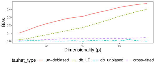
Errors: normal

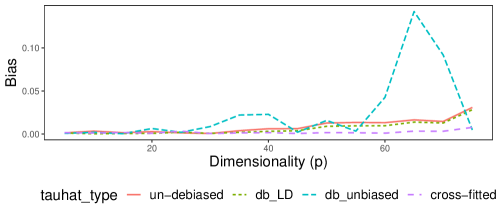
Figure B.1. Relative biases for $X\sim t(3)$ ($n=500$).

Errors: worst

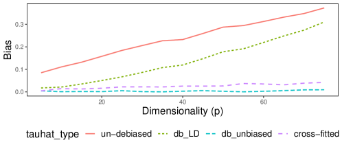
Errors: normal

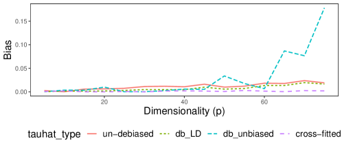
Figure B.2. Relative biases for $X\sim t(4)$ ($n=500$).

Covariates: $X\sim t(3)$

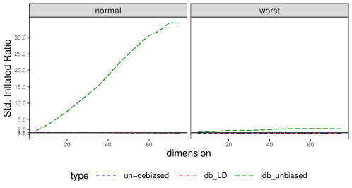
Covariates: $X\sim t(4)$

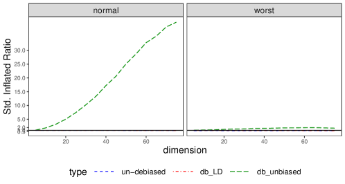
Figure B.3. Standard deviation of alternative estimators relative to the standard deviation of the cross-fitted estimator ($n=500$).

Covariates: $X\sim t(3)$

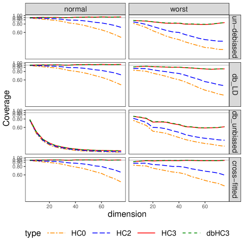
Covariates: $X\sim t(4)$

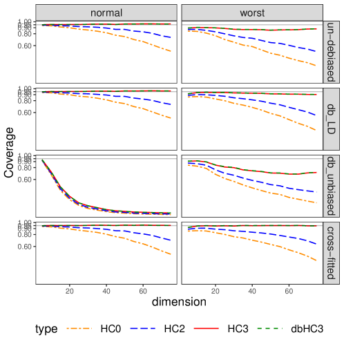
Figure B.4. Coverage rates ($n=500$).

Covariates: $X\sim t(3)$
 
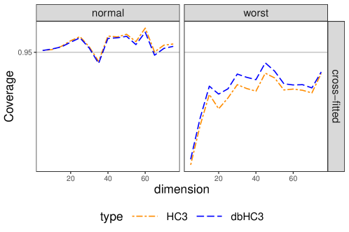
Covariates: $X\sim t(4)$

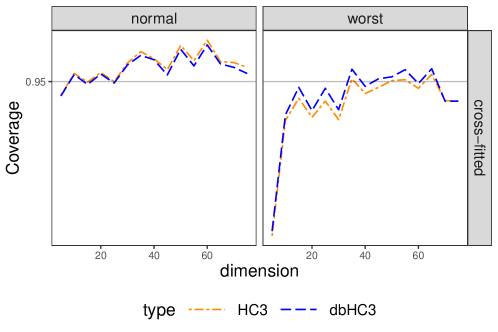
Figure B.5. Comparing coverage rates of HC3 and dbHC3 ($n=500$).

References

- (1)
- Abadie et al. (2020) Abadie, A., S. Athey, G. W. Imbens, and J. M. Wooldridge (2020): “Sampling-Based versus Design-Based Uncertainty in Regression Analysis,” Econometrica, 88, 265–296.
- Angrist et al. (2009) Angrist, J., D. Lang, and P. Oreopoulos (2009): “Incentives and services for college achievement: Evidence from a randomized trial,” American Economic Journal: Applied Economics, 1, 136–63.
- Aronow et al. (2014) Aronow, P. M., D. P. Green, and D. K. Lee (2014): “Sharp bounds on the variance in randomized experiments,” The Annals of Statistics, 42, 850–871.
- Bloniarz et al. (2016) Bloniarz, A., H. Liu, C.-H. Zhang, J. S. Sekhon, and B. Yu (2016): “Lasso adjustments of treatment effect estimates in randomized experiments,” Proceedings of the National Academy of Sciences, 113, 7383–7390.
- Bradic et al. (2019) Bradic, J., S. Wager, and Y. Zhu (2019): “Sparsity double robust inference of average treatment effects,” arXiv preprint arXiv:1905.00744.
- Cattaneo et al. (2019) Cattaneo, M. D., M. Jansson, and X. Ma (2019): “Two-step estimation and inference with possibly many included covariates,” The Review of Economic Studies, 86, 1095–1122.
- Cattaneo et al. (2018a) Cattaneo, M. D., M. Jansson, and W. K. Newey (2018a): “Alternative asymptotics and the partially linear model with many regressors,” Econometric Theory, 34, 277–301.
- Cattaneo et al. (2018b) by same author(2018b): “Inference in linear regression models with many covariates and heteroscedasticity,” Journal of the American Statistical Association, 113, 1350–1361.
- Chang et al. (2021) Chang, H., J. Middleton, and P. Aronow (2021): “Exact Bias Correction for Linear Adjustment of Randomized Controlled Trials,” arXiv preprint arXiv:2110.08425.
- Chernozhukov et al. (2018) Chernozhukov, V., D. Chetverikov, M. Demirer, E. Duflo, C. Hansen, W. Newey, and J. Robins (2018): “Double/debiased machine learning for treatment and structural parameters: Double/debiased machine learning,” The Econometrics Journal, 21.
- Dasgupta et al. (2015) Dasgupta, T., N. S. Pillai, and D. B. Rubin (2015): “Causal inference from 2K factorial designs by using potential outcomes,” Journal of the Royal Statistical Society: Series B (Statistical Methodology), 77, 727–753.
- Fisher (1925) Fisher, R. A. (1925): “Statistical methods for research workers.,” Statistical methods for research workers.
- Fisher (1935) by same author(1935): “1935. The Design of Experiments,” Edinburgh: Oliver and Boyd.
- Fogarty (2018) Fogarty, C. B. (2018): “Regression-assisted inference for the average treatment effect in paired experiments,” Biometrika, 105, 994–1000.
- Freedman (2008) Freedman, D. A. (2008): “On regression adjustments to experimental data,” Advances in Applied Mathematics, 40, 180–193.
- Hansen (2022) Hansen, B. (2022): Econometrics: Princeton University Press.
- Imbens and Menzel (2021) Imbens, G., and K. Menzel (2021): “A CAUSAL BOOTSTRAP,” Annals of Statistics, 49, 1460–1488.
- Imbens and Rubin (2015) Imbens, G. W., and D. B. Rubin (2015): Causal inference in statistics, social, and biomedical sciences: Cambridge University Press.
- Kempthorne (1952) Kempthorne, O. (1952): “The design and analysis of experiments..”
- Lei and Ding (2021) Lei, L., and P. Ding (2021): “Regression adjustment in completely randomized experiments with a diverging number of covariates,” Biometrika, 108, 815–828.
- Li and Ding (2020) Li, X., and P. Ding (2020): “Rerandomization and regression adjustment,” Journal of the Royal Statistical Society. Series B: Statistical Methodology, 82, 241–268.
- Li et al. (2018) Li, X., P. Ding, and D. B. Rubin (2018): “Asymptotic theory of rerandomization in treatment-control experiments,” Proceedings of the National Academy of Sciences, 115, 9157–9162.
- Lin (2013) Lin, W. (2013): “Agnostic notes on regression adjustments to experimental data: Reexamining Freedman’s critique,” Annals of Applied Statistics, 7, 295–318.
- Liu and Yang (2020) Liu, H., and Y. Yang (2020): “Regression-adjusted average treatment effect estimates in stratified randomized experiments,” Biometrika, 107, 935–948.
- Newey and Robins (2018) Newey, W. K., and J. R. Robins (2018): “Cross-fitting and fast remainder rates for semiparametric estimation,” arXiv preprint arXiv:1801.09138.
- Neyman (1923) Neyman, J. S. (1923): “On the application of probability theory to agricultural experiments. essay on principles. section 9.,” Annals of Agricultural Sciences, 10, 1–51.
- Reichardt and Gollob (1999) Reichardt, C. S., and H. F. Gollob (1999): “Justifying the use and increasing the power of at test for a randomized experiment with a convenience sample.,” Psychological methods, 4, 117.
- Rosenberger and Lachin (2015) Rosenberger, W. F., and J. M. Lachin (2015): Randomization in clinical trials: theory and practice: John Wiley & Sons.
- Schick (1986) Schick, A. (1986): “On asymptotically efficient estimation in semiparametric models,” Annals of Statistics, 1139–1151.
- Spiess (2018) Spiess, J. (2018): “Optimal estimation when researcher and social preferences are misaligned,” working paper.
- Tan (2014) Tan, Z. (2014): “Second-order asymptotic theory for calibration estimators in sampling and missing-data problems,” Journal of Multivariate Analysis, 131, 240–253.
- Wager et al. (2016) Wager, S., W. Du, J. Taylor, and R. J. Tibshirani (2016): “High-dimensional regression adjustments in randomized experiments,” Proceedings of the National Academy of Sciences, 113, 12673–12678.
- Wu and Gagnon-Bartsch (2018) Wu, E., and J. A. Gagnon-Bartsch (2018): “The LOOP estimator: Adjusting for covariates in randomized experiments,” Evaluation Review, 42, 458–488.
- Zheng and van der Laan (2011) Zheng, W., and M. J. van der Laan (2011): “Cross-validated targeted minimum-loss-based estimation,” in Targeted Learning: Springer, 459–474.