Analyzing Feed-Forward Blocks in Transformers through the Lens of Attention Map

Abstract

Given that Transformers are ubiquitous in wide tasks, interpreting their internals is a pivotal issue. Still, their particular components, feed-forward (FF) blocks, have typically been less analyzed despite their substantial parameter amounts. We analyze the input contextualization effects of FF blocks by rendering them in the attention maps as a human-friendly visualization scheme. Our experiments with both masked- and causal-language models reveal that FF networks modify the input contextualization to emphasize specific types of linguistic compositions. In addition, FF and its surrounding components tend to cancel out each other’s effects, suggesting potential redundancy in the processing of the Transformer layer.

1 Introduction

Transformers have been ubiquitous in a wide range of natural language processing tasks (Vaswani et al., 2017; Devlin et al., 2019; Radford et al., 2019; Brown et al., 2020); interpreting their inner workings is challenging and important to rationalize their outputs due to their black-box nature (Carvalho et al., 2019; Rogers et al., 2020; Braşoveanu & Andonie, 2020). In particular, tracking their component-by-component internal processing can provide rich information about their intermediate processing, given the stacked architecture of Transformer. With this motivation, existing studies have typically analyzed the role of each Transformer component or its specific subpart (Kobayashi et al., 2020; 2021; Modarressi et al., 2022). Taking the analyses of feed-forward (FF) networks as examples, Oba et al. (2021) explored the relationship between FF’s neuron activation and specific phrases, and Geva et al. (2021) and Dai et al. (2022) examined the knowledge stored in FF’s parameters through viewing FF as key-value memories.

Among the various approaches to interpreting the model’s internal processing, rendering $n\times n$ attention maps through attention mechanisms, where the $(i,j)$ cell represents how strongly a particular input $\bm{x}_{j}\in\{\bm{x}_{1},\ldots,\bm{x}_{n}\}$ contributed to a particular output $\bm{y}_{i}$, has gained certain popularity as a human-friendly interface (Braşoveanu & Andonie, 2020; Vig, 2019). Such maps are typically estimated with attention weights in each attention head (Clark et al., 2019; Kovaleva et al., 2019); this has an obvious limitation of only reflecting a specific process (QK attention computation) of the Transformer layer. Then, to tackle this limitation, existing studies refined the attention map computation to reflect other components’ processing, such as residual and normalization layers (Brunner et al., 2020; Abnar & Zuidema, 2020; Kobayashi et al., 2020; 2021; Modarressi et al., 2022), enabling us to look into other components through the rendered attention map. Notably, visualizing and refining attention maps have several advantages: (i) Attention mechanisms are spread out in the entire Transformer architecture; thus, if one can view their surrounding component’s processing through this “semi-transparent window,” these pictures can complete the Transformer’s component-by-component internal processing, (ii) token-to-token relationships are relatively more familiar to humans than directly observing high-dimensional, continuous intermediate representations/parameters, and input attribution is of major interest in explaining the model prediction, and (iii) it has been reported that such attention map refinement approaches tend to estimate better attributions than other, e.g., gradient-based methods (Modarressi et al., 2022; 2023).

Still, in this line of analyses towards input contextualization via attention map, FF networks have been overlooked from the analysis scope, although there are several motivations to consider FFs. For example, FFs account for about two-thirds of the layer parameters in typical Transformer-based models, such as BERT and GPT series; this implies that FF has the expressive power to dominate the model’s inner workings, and understanding such a large component’s processing is also related to pruning large models. In addition, there is a growing general interest in FFs with the rise of FF-focused methods such as adapters (Houlsby et al., 2019) and MLP-Mixer (Tolstikhin et al., 2021), although analyzing these specially designed models is beyond this paper’s focus. Furthermore, it has been reported that FFs indeed perform some linguistic operations, while existing studies have not explicitly focused on input contextualization(Geva et al., 2021; Dai et al., 2022).

In this study, we analyze the FF blocks in the Transformer layer, i.e., FF networks and their surrounding residual and normalization layers, with respect to their impact on input contextualization through the lens of attention map. Notably, although the FFs are applied to each input representation independently, their transformation can inherently affect the input contextualization (§ 3), and our experiments show that this indeed occurs (§ 5.1). Technically, we propose a method to compute attention maps reflecting the FF blocks’ processing by extending a norm-based analysis (Kobayashi et al., 2021), which has several advantages: the impact of input ($\lVert\bm{x}\rVert$) is considered unlike the vanilla gradient, and that only the forward computation is required. Although the original norm-based approach can not be simply applied to the non-linear part in the FF, this study handles this limitation by partially applying an integrated gradient (Sundararajan et al., 2017) and enables us to track the input contextualization from the information geometric perspectives.

Our experiments with both masked- and causal-language models (LMs) disclosed the contextualization effects of the FF blocks. Specifically, we first reveal that FF and layer normalization in specific layers tend to largely control contextualization. We also observe typical FF effect patterns, independent of the LM types, such as amplifying a specific type of lexical composition, e.g., subwords-to-word and words-to-multi-word-expression constructions (§ 5.2). Furthermore, we also first observe that the FF’s effects are weakened by surrounding residual and normalization layers (§ 6), suggesting redundancy in the Transformer’s internal processing.

2 Background

Notation: Boldface letters such as $\bm{x}$ denote row vectors.

Transformer layer: The Transformer architecture (Vaswani et al., 2017) consists of a series of layers, each of which updates each token representation $\bm{x}_{i}\in\mathbb{R}^{d}$ in input sequence $\bm{X}\coloneqq[\bm{x}^{\top}_{1},\ldots,\bm{x}^{\top}_{n}]^{\top}\in\mathbb{R}^{n\times d}$ to a new representation $\bm{y}_{i}\in\mathbb{R}^{d}$. Each layer is composed of four parts: multi-head attention (ATTN), feed-forward network (FF), residual connection (RES), and layer normalization (LN) (see Fig. 1). Note that we use the Post-LN architecture (Vaswani et al., 2017) for the following explanations in this paper, but the described methods can simply be extended to the Pre-LN variant (Xiong et al., 2020). A single layer can be written as a composite function:

$$\bm{y}_{i} \!=\!\mathrm{Layer}(\bm{x}_{i};\!\bm{X})\!=\!(\mathrm{FFB}\circ\!\mathrm{ATB})(\bm{x}_{i};\!\bm{X})\!=\!(\mathrm{LN2}\circ\mathrm{RES2}\circ\mathrm{FF}\!\circ\mathrm{LN1}\circ\mathrm{RES1}\circ\!\mathrm{ATTN})(\bm{x}_{i};\!\bm{X})\text{.}$$

We call $(\mathrm{LN1}\circ\mathrm{RES1}\circ\mathrm{ATTN})(\cdot)$ attention block (ATB), and $(\mathrm{LN2}\circ\mathrm{RES2}\circ\mathrm{FF})(\cdot)$ feed-forward block (FFB). Each component updates the representation as follows:

$$\mathrm{ATTN}(\bm{x}_{i};\bm{X})=\textstyle(\sum_{h}\sum_{j}\alpha^{h}_{i,j}\bm{x}_{j}\bm{W}_{V}+\bm{b}_{V})\bm{W}_{O}+\bm{b}_{O}\in\mathbb{R}^{d}$$ (1)

$$\quad\text{where}\quad\alpha^{h}_{i,j}\coloneqq(\bm{x}_{i}\bm{W}_{Q}+\bm{b}_{Q})(\bm{x}_{i}\bm{W}_{K}+\bm{b}_{K})^{\top}\in\mathbb{R}$$ (2)

$$\mathrm{FF}(\bm{z}_{i})=\bm{g}(\bm{z}_{i}\bm{W}_{1}+\bm{b}_{1})\bm{W}_{2}+\bm{b}_{2}\in\mathbb{R}^{d}$$ (3)

$$(\mathrm{RES}\circ\bm{f})(\bm{z}_{i})=\bm{f}(\bm{z}_{i})+\bm{z}_{i}\in\mathbb{R}^{d}$$ (4)

$$\mathrm{LN}(\bm{z}_{i})=\frac{\bm{z}_{i}-m(\bm{z}_{i})}{s(\bm{z}_{i})}\odot\bm{\gamma}+\bm{\beta}\in\mathbb{R}^{d}\text{,}$$ (5)

where $\bm{W},\bm{\gamma}$ denote weight parameters, and $\bm{b},\bm{\beta}$ denote bias parameters corresponding to query (Q), key (K), value (V), etc. $\bm{f}\colon\mathbb{R}^{d}\to\mathbb{R}^{d}$, $\bm{g}\colon\mathbb{R}^{d^{\prime}}\to\mathbb{R}^{d^{\prime}}$, $m\colon\mathbb{R}^{d}\to\mathbb{R}$, and $s\colon\mathbb{R}^{d}\to\mathbb{R}$ denote an arbitrary vector-valued function, activation function in FF (e.g., GELU, Hendrycks & Gimpel, 2016), element-wise mean, and element-wise standard deviation, respectively. $h$ denotes the head number in the multi-head attention. See the original paper (Vaswani et al., 2017) for more details.

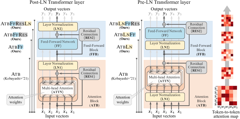
Figure 1: Overview of the Transformer layer for Post-LN and Pre-LN architectures. The block diagram to the left of each represents the analysis scope adopted in this study. The right part of this figure illustrates the component-by-component changes of the attention maps.

Attention map: Our interest lies in how strongly each input $\bm{x}_{j}$ contributes to the computation of a particular output $\bm{y}_{i}$. This is typically visualized as an $n\times n$ attention map, where the $(i,j)$ cell represents how strongly $\bm{x}_{j}$ contributed to compute $\bm{y}_{i}$. A typical approximation of such a map is facilitated with the attention weights ($\alpha^{h}_{i,j}$ or $\sum_{h}\alpha^{h}_{i,j}$; henceforth denoted $\alpha_{i,j}$) (Clark et al., 2019; Kovaleva et al., 2019); however, this only reflects a specific process (QK attention computation) of the Transformer layer (Brunner et al., 2020; Kobayashi et al., 2020; Abnar & Zuidema, 2020).

Looking into Transformer layer through attention map: Nevertheless, an attention map is not only for visualizing the attention weights; existing studies (Kobayashi et al., 2020; 2021) have analyzed other components through the lens of refined attention map. Specifically, Kobayashi et al. (2020) pointed out that the processing in the multi-head QKV attention mechanism can be written as a sum of transformed vectors:

$$\bm{y}_{i}^{\mathrm{ATTN}}=\textstyle\sum_{j}\bm{F}^{\mathrm{ATTN}}_{i}(\bm{x}_{j};\bm{X})+\bm{b}^{\mathrm{ATTN}}\text{,}$$ (6)

$$\text{where}\quad\bm{F}^{\mathrm{ATTN}}_{i}(\bm{x}_{j};\bm{X})\coloneqq\alpha_{i,j}^{h}(\bm{x}_{j}\bm{W}_{V}^{h})\bm{W}_{O}^{h}\text{,}\quad\bm{b}^{\mathrm{ATTN}}\coloneqq\bm{b}_{V}\bm{W}_{O}+\bm{b}_{O}\text{.}$$ (7)

Here, input representation $\bm{x}_{i}$ is updated to $\bm{y}^{\mathrm{ATTN}}_{i}$ by aggregating transformed inputs $\bm{F}^{\mathrm{ATTN}}_{i}(\bm{x}_{j};\bm{X})$. Then, $\lVert\bm{F}^{\mathrm{ATTN}}_{i}(\bm{x}_{j};\bm{X})\rVert$ instead of $\alpha_{i,j}$ alone is regarded as refined attention weight with the simple intuition that larger input contributes to output more in summation. This refined weight reflects not only the original attention weight $\alpha_{i,j}$, but also the effect of surrounding processing involved in $\bm{F}$, such as value vector transformation. We call this strategy of decomposing the process into the sum of transformed vectors and measuring their norms norm-based analysis, and the obtained $n\times n$ attribution matrix is generally called attention map in this study.

This norm-based analysis has been further generalized to a broader component of the Transformer layer. Specifically, Kobayashi et al. (2021) showed that the operation of attention block (ATB) could also be rewritten into the sum of transformed inputs and a bias term:

$$\bm{y}_{i}^{\mathrm{ATB}} =\mathrm{ATB}(\bm{x}_{i};\bm{X})=\textstyle\sum_{j}\bm{F}^{\mathrm{ATB}}_{i}(\bm{x}_{j};\bm{X})+\bm{b}^{\mathrm{ATB}}\text{.}$$ (8)

Then, the norm $\lVert\bm{F}^{\mathrm{ATB}}_{i}(\bm{x}_{j};\bm{X})\rVert$ was analyzed to quantify how much the input $\bm{x}_{j}$ impacted the computation of the output $\bm{y}_{i}^{\mathrm{ATB}}$ through the ATBs. See Appendix A for details of $\bm{F}^{\mathrm{ATB}}_{i}$ and $\bm{b}^{\mathrm{ATB}}$.

3 Proposal: analyzing FFBs through refined attention map

The transformer layer is not only an ATB; it consists of an ATB and FFB (Figs. 1 and 2). Thus, this study broadens the analysis scope to include the entire FF block consisting of feed-forward, residual, and normalization layers, in addition to the ATB. Note that FFBs do not involve token-wise interaction among the inputs $\bm{X}$; thus, the layer output $\bm{y}_{i}^{\mathrm{Layer}}$ can be written as transformed $\bm{y}_{i}^{\mathrm{ATB}}$. Then, our aim is to decompose the entire layer processing as follows:

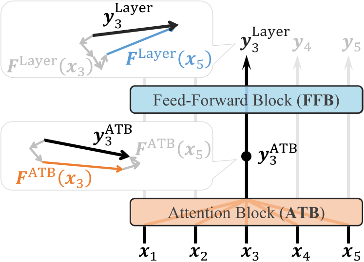
Figure 2: An illustration of possible contextualization effects by FFB. The FFB does not have the function of mixing input tokens together; however, its input already contain mixed information from multiple tokens, and the FFB is capable of altering these weights. Here, output $\bm{y}_{3}$ is computed based on $[\bm{x}_{1},\cdots,\bm{x}_{5}]$. Based on the vector norm, the most influential input seems to be $\bm{x}_{3}$ before FF; however, after the FF’s transformation, $\bm{x}_{5}$ becomes the most influential input.

$$\bm{y}_{i}^{\mathrm{Layer}} =\textstyle\mathrm{FFB}\bigl{(}\sum_{j}\bm{F}_{i}^{\mathrm{ATB}}(\bm{x}_{j};\bm{X})+\bm{b}^{\mathrm{ATB}}\bigr{)}$$ (9)

$$\textstyle=\sum_{j}\bm{F}_{i}^{\mathrm{Layer}}(\bm{x}_{j};\bm{X})+\bm{b}^{\mathrm{Layer}}\text{.}$$ (10)

Here, the norm $\lVert\bm{F}^{\mathrm{Layer}}_{i}(\bm{x}_{j};\bm{X})\rVert$ can render the updated attention map reflecting the processing in the entire layer. This attention map computation can also be performed component-by-component; we can track each FFB component’s effect.

Why FFBs can control contextualization patterns: While FFBs are applied independently to each input representation, FFB’s each input already contains mixed information from multiple token representations due to the ATB’s process, and the FFBs can freely modify these weights through a nonlinear transformation (see Fig. 2).

Difficulty to incorporate FF: While FFBs have the potential to significantly impact contextualization patterns, incorporating the FF component into norm-based analysis is challenging due to its nonlinear activation function, $\bm{g}$ (Eq. 3), which cannot be decomposed additively by the distributive law:

$$\textstyle\bm{g}\Bigl{(}\sum_{j}\bm{F}(\bm{x}_{j})\Bigr{)}\neq\sum_{j}(\bm{g}\circ\bm{F})(\bm{x}_{j})\text{.}$$ (11)

This inequality matters in the transformation from Eq. 9 to Eq. 10. That is, simply measuring the norm $\lVert(\bm{g}\circ\bm{F})(\bm{x}_{j})\rVert$ is not mathematically valid. Indeed, the FF component has been excluded from previous norm-based analyses. Note that the other components in FFBs, residual connection and layer normalization, can be analyzed in the same way proposed in Kobayashi et al. (2021).

Integrated Gradients (IG): The IG (Sundararajan et al., 2017) is a technique for interpreting deep learning models by using integral and gradient calculations. It measures the contribution of each input feature to the output of a neural model. Given a function $f\colon\mathbb{R}^{n}\to\mathbb{R}$ and certain input $\bm{x}^{\prime}=(x^{\prime}_{1},\dots,x^{\prime}_{n})\in\mathbb{R}^{n}$, IG calculates the contribution (attribution) score ($\in\mathbb{R}$) of each input feature $x^{\prime}_{i}\in\mathbb{R}$ to the output $f(\bm{x}^{\prime})\in\mathbb{R}$:

$$f(\bm{x}^{\prime})=\sum_{j=1}^{n}\mathrm{IG}_{j}(\bm{x}^{\prime};f,\bm{b})+f(\bm{b})\text{,}\quad\mathrm{IG}_{i}(\bm{x}^{\prime};f,\bm{b})\coloneqq(x^{\prime}_{i}-b_{i})\int_{\alpha=0}^{1}\frac{\partial f}{\partial x_{i}}\bigg{\rvert}_{\bm{x}\,=\,\bm{b}\,+\,\alpha(\bm{x}^{\prime}\,-\,\bm{b})}\mathrm{d}\alpha\text{.}\!\!$$ (12)

Here, $\bm{b}\in\mathbb{R}^{n}$ denotes a baseline vector used to estimate the contribution. At least in this study, it is set to a zero vector, which makes zero output when given into the activation function ($\bm{g}(\bm{0})=\bm{0}$), to satisfy desirable property for the decomposition (see Appendix B.2 for details).

Expansion to FF: We explain how to use IG for the decomposition of FF output. As aforementioned, the problem lies in the nonlinear part, thus we focus on the decomposition around the nonlinear activation. Let us define $\bm{F}^{\text{Pre }g}_{i}(\bm{x}_{j})\coloneqq\bm{F}^{\mathrm{ATB}}_{i}(\bm{x}_{j};\bm{X})\bm{W}_{1}\in\mathbb{R}^{d^{\prime}}$ as the decomposed vector prior to the nonlinear activation $\bm{g}\colon\mathbb{R}^{d^{\prime}}\to\mathbb{R}^{d^{\prime}}$. The activated token representation $\bm{y}^{\prime}\in\mathbb{R}^{d^{\prime}}$ is written as follows:

$$\textstyle\bm{y}^{\prime}_{i}=\bm{g}\Biggl{(}\sum_{j=1}^{n}\bm{F}^{\text{Pre }g}_{i}(\bm{x}_{j})\Biggr{)}=\sum_{j=1}^{n}\bm{h}_{j}\bigl{(}\bm{F}^{\text{Pre }g}_{i}(\bm{x}_{1}),\ldots,\bm{F}^{\text{Pre }g}_{i}(\bm{x}_{n});\widetilde{g},\bm{0}\bigr{)}\text{,}$$ (13)

$$\bm{h}_{j}\bigl{(}\bm{F}^{\text{Pre }g}_{i}(\bm{x}_{1}),\ldots,\bm{F}^{\text{Pre }g}_{i}(\bm{x}_{n});\widetilde{g},\bm{0}\bigr{)}=\begin{bmatrix}\mathrm{IG}_{j}\Bigl{(}\bm{F}^{\text{Pre }g}_{i}(\bm{x}_{1})[1],\dots,\bm{F}^{\text{Pre }g}_{i}(\bm{x}_{n})[1];\widetilde{g},\bm{0}\Bigr{)}\\ \vdots\\ \mathrm{IG}_{j}\Bigl{(}\bm{F}^{\text{Pre }g}_{i}(\bm{x}_{1})[d^{\prime}],\dots,\bm{F}^{\text{Pre }g}_{i}(\bm{x}_{n})[d^{\prime}];\widetilde{g},\bm{0}\Bigr{)}\end{bmatrix}^{\!\top}\!\!\!\text{,}$$ (14)

where the transformation $\widetilde{g}\colon\mathbb{R}^{n}\to\mathbb{R}$ is defined as $\widetilde{g}(x_{1},\dots,x_{n})\coloneqq g(x_{1}+\dots+x_{n})$, which adds up the inputs into a single scalar and then applies the element-level activation $g\colon\mathbb{R}\to\mathbb{R}$. The function $\bm{h}_{j}\colon\mathbb{R}^{n\times d^{\prime}}\to\mathbb{R}^{d^{\prime}}$ yields how strongly a particular input $\bm{F}^{\text{Pre }g}_{i}(\bm{x}_{j})$ contributed to the output $\bm{y}^{\prime}_{i}$. Each element $\bm{h}_{j}[k]$ indicates the contribution of the $k$-th element of input $\bm{F}^{\text{Pre }g}_{i}(\bm{x}_{j})[k]$ to the $k$-th element of output $\bm{y}^{\prime}_{i}[k]$. Note that contribution can be calculated element-level because the activation $g$ is applied independently to each element.

Notably, the sum of contributions across inputs matches the output (Eq. 13), achieved by the desirable property of IG—completeness Sundararajan et al. (2017). This should be satisfied in the norm-based analysis and ensures that the output vector and the sum of decomposed vectors are the same. The norm $\lVert\bm{h}_{j}(\bm{F}_{i}^{\text{Pre }g}(\bm{x}_{1}),\ldots,\bm{F}_{i}^{\text{Pre }g}(\bm{x}_{n});\widetilde{g},\bm{0})\rVert$ is interpreted as the contribution of input $\bm{x}_{j}$ to the output $\bm{y}^{\prime}_{i}$ of the activation in FF.

Expansion to entire layer: Expanding on this, the contribution of a layer input $\bm{x}_{j}$ to the $i$-th FF output is exactly calculated as $\lVert\bm{h}_{j}(\bm{F}_{i}^{\text{Pre }g}(\bm{x}_{1}),\ldots,\bm{F}_{i}^{\text{Pre }g}(\bm{x}_{n});\widetilde{g},\bm{0})\bm{W}_{2}\rVert$. Then, combined with the exact decomposition of ATTN, RES, and LN shown by Kobayashi et al. (2020; 2021), the entire Transformer layer can be written as the sum of vector-valued functions with each input vector $\bm{x}_{j}\in\bm{X}$ as an argument as written in Eq. 10. This allows us to render the updated attention map reflecting the processing in the entire layer by measuring the norm of each decomposed vector.

4 General experimental settings

Estimating refined attention map: To elucidate the input contextualization effect of each component in FFBs, we computed attention maps by each of the following four scopes (Fig. 1):

• Atb (Kobayashi et al., 2021): Analyzing the attention block (i.e., ATTN, RES1, and LN1) using vector norms as introduced in Eq. 8.

• AtbFf (proposed): Analyzing components up to FF using vector norms and IG.

• AtbFfRes (proposed): Analyzing components up to RES2 using vector norms and IG.

• AtbFfResLn (proposed): Analyzing the whole layer (all components) using vector norms and IG.

We will compare the attention maps from different scopes to separately analyze the contextualization effect. Note that if the model adopts the Pre-LN architecture, the scopes will be expanded from Atb to AtbLn, AtbLnFf, and AtbLnFfRes (see the Pre-LN part in Fig. 1).

Models: We analyzed $11$ variants of the masked language models: six BERTs (uncased) with different sizes (large, base, medium, small, mini, and tiny) (Devlin et al., 2019; Turc et al., 2019), three BERTs-base with different seeds (Sellam et al., 2022), plus two RoBERTas with different sizes (large and base) (Liu et al., 2019). We also analyze one causal language model (GPT-2 with 117M parameters) to examine the generality of our findings. Note that the masked language models adopt the Post-LN architecture, and the causal language model adopts the Pre-LN architecture.

Data: We used two datasets with different domains: Wikipedia excerpts (992 sequences) (Clark et al., 2019) and the Stanford Sentiment Treebank v2 dataset (872 sequences from validation set) (SST-2, Socher et al., 2013). The input was segmented by each model’s pre-trained tokenizers; analysis was conducted at the subword level.

5 Experiment 1: Contextualization change

Does each component in FFBs indeed modify the token-to-token contextualization? We analyze the contextualization change through each component in FFBs.

5.1 Macro contextualization change

Calculating contextualization change: Given two analysis scopes (e.g., before and after FF; Atb $\leftrightarrow$ AtbFf), their contextualization pattern change was quantified following some procedures of representational similarity analysis (Kriegeskorte et al., 2008). Formally, given an input sequence of length $n$, two different attention maps from the two scopes are obtained. Then, each attention map ($\mathbb{R}^{n\times n}$) was flattened into a vector ($\mathbb{R}^{n^{2}}$), and the Spearman’s rank correlation coefficient $\rho$ between the two vectors were calculated. We report the average contextualization change $1-\rho$ across input sequences. We will report the results of the BERT-base and GPT-2 on the Wikipedia dataset in this section; other models/datasets also yielded similar results (see Appendix C.1).

The contextualization changes through each component in FFBs are shown in Fig. 3. A higher score indicates that the targeted component more drastically updates the contextualization patterns. Note that we explicitly distinguish the pre- and post-layer normalization (Preln and Postln) in this section, and the component order in Fig. 3 is the same as the corresponding layer architecture.

BERT (PostLN)

(a) +Ff
(Atb $\leftrightarrow$ AtbFf)

(b) +Res
(AtbFf $\leftrightarrow$ AtbFfRes)

(c) +Ln
(AtbFfRes $\leftrightarrow$ AtbFfResLn)

GPT-2 (PreLN)

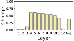
(d) +Ln
(Atb $\leftrightarrow$ AtbLn)

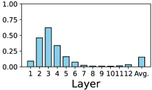
(e) +Ff
(AtbLn $\leftrightarrow$ AtbLnFf)

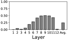
(f) +Res
(AtbLnFf $\leftrightarrow$ AtbLnFfRes)

Figure 3: Contextualization changes between before and after each component in FFBs (FF, RES2, and LN2) of BERT and GPT-2. The higher the bar, the more drastically the token-to-token contextualization (attention maps) changes due to the target component.

We generally observed that each component did modify the input contextualization, especially in particular layers. For example, in the BERT-base, the FF in $3$rd and $9$th–$11$th layers and normalization in $10$th–$11$th layers incurred relatively large contextualization change. Comparing the BERT-base and GPT-2, the depth of such active layers and the account of Res differed, but by-layer average of contextualization change by Ff and Ln was similar across these LMs: $0.21$ and $0.15$ for Ff in BERT and GPT-2, respectively, and $0.27$ and $0.38$ for Ln in BERT and GPT-2, respectively. Note that Figures 9 to 12 in Appendix C show the results for other model variants, yielding somewhat consistent trends that FFs and LNs in the middle to latter layers incur more contextualization changes.

5.2 Linguistic patterns in FF’s contextualization effects

The FF network is a completely new scope in the norm-based analysis, while residual and normalization layers have been analyzed in Kobayashi et al. (2021); Modarressi et al. (2022). Thus, we further investigate how FF modified contextualization, using BERT-base and GPT-2 on the Wikipedia dataset as a case study.

Micro contextualization change: We compared the attention maps before and after FF. Specifically, we subtract a pre-FF attention map from a post-FF map (Fig. 4); we call the resulting diff-map FF-amp matrix and the values in each cell FF-amp score. A larger FF-amp score of the ($i$, $j$) cell

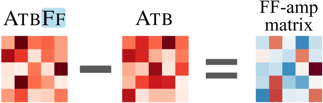
Figure 4: FF-amp matrix is computed by subtracting the attention map before FF (Atb) from that after FF (AtbFf).

presents that the contribution of input $\bm{x}_{j}$ to output $\bm{y}_{i}$ is more amplified by FF. Our question is which kind of token pairs gain a higher FF-amp score.

FFs amplify particular linguistic compositions: Based on the preliminary observations of high FF-amp token pairs, we set 7 linguistic categories typically amplified by FFBs. This includes, for example, token pairs consisting of the same words but different positions in the input. Table 1 shows the top token pairs w.r.t. the amp score in some layers and their token pair category. Fig. 5 summarizes the ratio of each category in the top 50 token pairs with the highest FF-amp score. Compared to the categories for randomly sampled token pairs (FR; the second rightmost bar in Fig. 5) and adjacent token pairs (AR; the rightmost bar in Fig. 5), the amplified pairs in each layer have unique characteristics; for example, in the former layers, subword pairs consisting the same token are highly contextualized by FFs. Note that this phenomenon of processing somewhat shallow morphological information in the former layers can be consistent with the view of BERT as a pipeline perspective, with gradually more advanced processing from the former to the latter layers Tenney et al. (2019).

Table 1: Token pairs sampled from the top 10 most-amplified subword pairs by FF in each layer of BERT (left) and GPT-2 (right). See Tables 2 and 3 in Appendix C.2 for the full pairs. The text colors are aligned with word pair categories, and the same colors are used in Fig. 5.

Layer	amplified pairs by BERT’s FF
1	(opera, soap), (##night, week)
3	(toys, ##hop), (’, t)
6	(with, charged), (fleming, colin)
9	(but, difficulty), (she, teacher)
11	(tiny, tiny), (highway, highway)

Layer	amplified pairs by GPT-2’s FF
1	(ies, stud), (ning, begin)
3	(_than, _rather), (_others, _among)
6	(_del, del), (_route, route)
8	(_08, _2007), (_14, _density)
12	(_operational, _not), (_daring, _has)

Figure 5: Breakdown of the category labels we manually assigned to top 50 pairs having the largest FF-amp score in each layer of BERT and GPT-2. We also assigned the labels to fully random 50 pairs (“FR”) and adjacent random 50 pairs (“AR”).

Simple word co-occurrence does not explain the FF’s amplification:

Do FFs simply amplify the interactions between frequently co-occurring words? We additionally investigated the relationship between the FF’s amplification and word co-occurrence. Specifically, we calculated PMI for each subword pair on the Wikipedia dump and then calculated the Spearman’s rank correlation coefficient between FF-amp scores of each pair $(w_{i},w_{j})$ from BERT-base and PMI values. We observed that the correlation scores were fairly low in any layer (coefficient values were $0.06$–$0.14$). Thus, we found that the FF does not simply modify the contextualization based on the word co-occurrence.

To sum up, these findings indicate that FF did amplify the contextualization aligned with particular types of linguistic compositions in various granularity (i.e., word and NE phrase levels).

6 Experiment 2: Dynamics of contextualization change

We analyze the relationship between the contextualization performed by FF and other components, such as RES, given the previous observation that contextualization changes in a particular component are sometimes overwritten by other components (Kobayashi et al., 2021). We will report the results of the BERT-base and GPT-2 on the Wikipedia dataset in this section; other models/datasets also yielded similar results (see Appendix D).

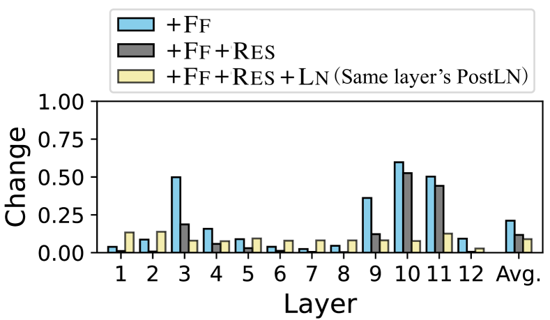
(a) BERT.

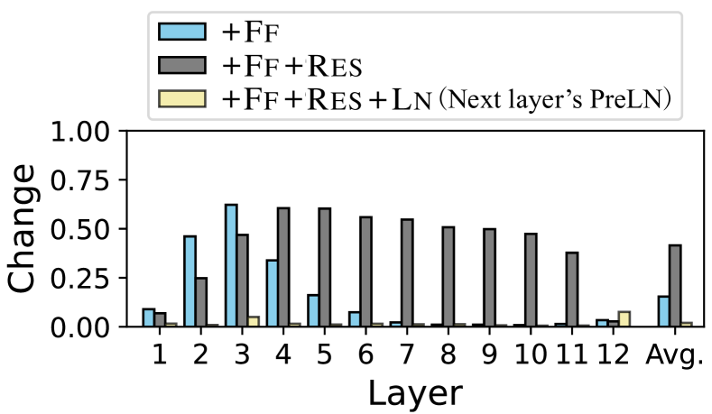
(b) GPT-2.

Figure 6: Contextualization changes through FF, RES, and LN relative to the contextualization performed before FF. The higher the bar, the more the contextualization changes.

Fig. 6 shows the contextualization change scores ($1-\rho$ described in § 5.1) by FF and subsequent components: FF (+FF), FF and RES (FF+RES), and FF, RES and LN (FF+RES+LN). Note that we analyzed the next-layer’s LN1 in the case of GPT2 (Pre-LN architecture) to analyze the BERTs and GPTs from the same perspective—whether the other components overwrite the contextualization performed in the FF network. If a score is zero, the resulting contextualization map is the same as that computed before FF (after ATBs in BERT or after LN2 in GPT-2). The notable point is that through the FF and subsequent RES and LN, the score once becomes large but finally converges to be small; that is, the contextualization by FFs tends to be canceled by the following components. We look into this cancellation phenomenon with a specific focus on each component.

6.1 FF and RES

The residual connection bypasses the feed-forward layer as Eq. 4. Here, the interest lies in how dominant the bypassed representation $\bm{x}^{\prime}_{i}$ is relative to $\mathrm{FF}(\bm{x}^{\prime}_{i})$. For example, if the representation $\bm{x}^{\prime}_{i}$ has a much larger L2 norm than $\mathrm{FF}(\bm{x}^{\prime}_{i})$, the final output through the $\mathrm{RES2}\circ\mathrm{FF}$ will be similar to the original input $\bm{x}^{\prime}_{i}$; that is, the contextualization change performed in the FF would be diminished.

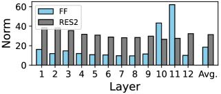
(a) BERT.

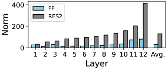
(b) GPT-2.

Figure 7: Averaged norm of the output vectors from FF and the bypassed vectors via RES2, calculated on the Wikipedia data for BERT and GPT-2.

RES2 adds a large vector: We observe that the vectors bypassed via RES2 are more than twice as large as output vectors from FF in the L2 norm in most layers (Fig. 7). That is, the representation (contextualization) updated by the FF tends to be overwritten/canceled by the original one. This observation is consistent with that of RES1 (Kobayashi et al., 2021). Notably, this cancellation is weakened in the $10$th–$11$th layers in BERT and former layers in GPT2s, where FFs’ contextualization was relatively large (Figs. 3 and 3).

6.2 FF and LN

We also analyzed the relationship between the contextualization performed in FF and LN. Note that the layer normalization first normalizes the input representation, then multiplies a weight vector $\bm{\gamma}$ element-wise, and adds a bias vector $\bm{\beta}$ (Eq. 8).

Cancellation mechanism: Again, as shown in Fig. 6, the contextualization change after the LN (+FF+RES+LN) is much lower than in preceding scopes (+FF and +FF+RES). That is, the LNs substantially canceled out the contextualization performed in the preceding components of FF and RES. Then, we specifically tackle the question, how did LN cancel the FF’s effect?

We first found that the FF output representation has outliers in some specific dimensions (green lines in Fig. 8), and that the weight $\bm{\gamma}$ of LN tends to shrink these special dimensions (red lines in Fig. 8). In the layers where FF incurs a relatively large impact on contextualization, the Pearson correlation coefficient between LN’s $\bm{\gamma}$ and mean absolute value of FF output by dimension was from $-0.45$ to $-0.78$ in BERTs and from $-0.22$ to $-0.59$ in GPT-2 across layers. Thus, we suspect that such specific outlier dimensions in the FF outputs encoded “flags” for potential contextualization change, and LN typically declines such FF’s suggestions by erasing the outliers.

(a) $10$th layer in BERT.

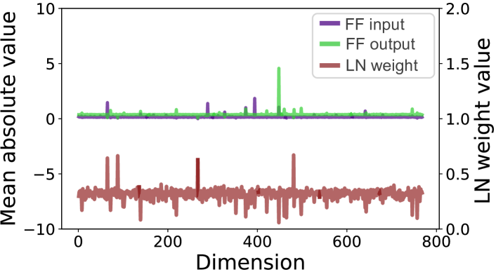
(b) $4$th layer in GPT-2.

Figure 8: Mean absolute value in each dimension of the input/output vectors of FF across the Wikipedia data and the LN weight values at the certain layer.

Indeed, we observed that ignoring such special outlier dimensions (bottom $1\%$ with the lowest value of $\bm{\gamma}$) in calculating FF’s contextualization makes the change score quite small; contextualization changes by FF went from $0.21$ to $0.09$ in BERT and from $0.15$ to $0.02$ in GPT-2 on a layer average. Thus, FF’s contextualization effect is realized using very specific dimensions, and LN2 cancels the effect by shrinking these special dimensions. Note that a related phenomenon was discovered by Modarressi et al. (2022): LN2 and LN1 cancel each other out by outliers in their weights in BERT. These imply, at least based only on existing observations, that the Transformer layer seems to perform redundant contextualization processing.

7 Conclusions and future work

We have analyzed the FF blocks w.r.t. input contextualization through the lens of a refined attention map by leveraging the existing norm-based analysis and the integrated gradient method having an ideal property—completeness. Our experiments using masked- and causal-language models have shown that FFs indeed modify the input contextualization by amplifying specific types of linguistic compositions (e.g., subword pairs forming one word). We have also found that FF and its surrounding components tend to cancel out each other’s contextualization effects and clarified their mechanism, implying the redundancy of the processing within the Transformer layer. Applying our analysis to other model variants, such as OPT (Zhang et al., 2022) and LLaMA (Touvron et al., 2023a; b)) families or LMs with FF-based adapters, will be our future work. In addition, focusing on inter-layer contextualization dynamics could also be fascinating future directions.

Appendix A Detailed formulas for each analysis method

We describe the mathematical details of the norm-based analysis methods adopted in this paper.

A.1 Atb

As described in § 2, Kobayashi et al. (2021) rewrite the operation of the attention block (ATB) into the sum of transformed inputs and a bias term:

$$\bm{y}_{i}^{\mathrm{ATB}} =\mathrm{ATB}(\bm{x}_{i};\bm{X})$$ (15)

$$=\mathrm{LN1}\circ\mathrm{RES1}\circ\mathrm{ATTN}$$ (16)

$$=\sum_{j=1}^{n}\bm{F}^{\mathrm{ATB}}_{i}(\bm{x}_{j};\bm{X})+\bm{b}^{\mathrm{ATB}}\text{.}$$ (17)

First, the multi-head attention mechanism (ATTN; Eq. 1) can be decomposed into a sum of transformed vectors as Eq. 6 and Eq. 7:

$$\mathrm{ATTN}(\bm{x}_{i};\bm{X}) =\sum_{j}\sum_{h}\alpha_{i,j}^{h}(\bm{x}_{j}\bm{W}_{V}^{h})\bm{W}_{O}^{h}+\bm{b}_{V}\bm{W}_{O}+\bm{b}_{O}$$ (18)

$$=\sum_{j}\bm{F}^{\mathrm{ATTN}}_{i}(\bm{x}_{j};\bm{X})+\bm{b}^{\mathrm{ATTN}}$$ (19)

$$\bm{F}^{\mathrm{ATTN}}_{i}(\bm{x}_{j};\bm{X})=\alpha_{i,j}^{h}(\bm{x}_{j}\bm{W}_{V}^{h})\bm{W}_{O}^{h}$$ (20)

$$\bm{b}^{\mathrm{ATTN}}=\bm{b}_{V}\bm{W}_{O}+\bm{b}_{O}\text{.}$$ (21)

Second, the residual connection (RES; Eq. 4) just performs the vector addition. So, ATTN and RES also can be decomposed into a sum of transformed vectors collectively:

$$(\mathrm{RES1}\circ\mathrm{ATTN})(\bm{x}_{i};\bm{X}) =\mathrm{ATTN}(\bm{x}_{i};\bm{X})+\bm{x}_{i}$$ (22)

$$=\sum_{j\neq i}\bm{F}^{\mathrm{ATTN}}_{i}(\bm{x}_{j};\bm{X})+\bm{x}_{i}+\bm{b}^{\mathrm{ATTN}}$$ (23)

$$=\sum_{j}\bm{F}^{\mathrm{ATTN+RES}}_{i}(\bm{x}_{j};\bm{X})+\bm{b}^{\mathrm{ATTN}}$$ (24)

$$\bm{F}^{\mathrm{ATTN+RES}}_{i} (\bm{x}_{j};\bm{X})=\left\{\begin{array}[]{ll}\bm{F}^{\mathrm{ATTN}}_{i}(\bm{x}_{j};\bm{X})&(j\neq j)\\ \bm{F}^{\mathrm{ATTN}}_{i}(\bm{x}_{i};\bm{X})+\bm{x}_{i}&(j=i)\end{array}\right.\text{.}$$ (27)

Third, the layer normalization (LN; Eq. 5) performs a normalization and element-wise affine transformation. Suppose the input to LN is a sum of vectors $\bm{z}=\sum_{j}\bm{z}_{j}$, LN’s operation is decomposed as follows:

$$\mathrm{LN}(\bm{z}) =\frac{\bm{z}-m(\bm{z})}{s(\bm{z})}\odot\bm{\gamma}+\bm{\beta}$$ (28)

$$=\frac{\bm{z}-\frac{1}{d}\sum_{k=1}^{d}\bm{z}^{(k)}}{s(\bm{z})}\odot\bm{\gamma}+\bm{\beta}$$ (29)

$$=\frac{\sum_{j}\bm{z}_{j}-\frac{1}{d}\sum_{k=1}^{d}\bigl{(}\sum_{j}\bm{z}_{j}\bigr{)}^{(k)}}{s(\bm{z})}\odot\bm{\gamma}+\bm{\beta}$$ (30)

$$=\sum_{j}\frac{\bm{z}_{j}-\frac{1}{d}\sum_{k=1}^{d}\bm{z}_{j}^{(k)}}{s(\bm{z})}\odot\bm{\gamma}+\bm{\beta}$$ (31)

$$=\sum_{j}\frac{\bm{z}_{j}-m(\bm{z}_{j})}{s(\bm{z})}\odot\bm{\gamma}+\bm{\beta}$$ (32)

$$=\sum_{j}\bm{F}^{\mathrm{LN}}(\bm{z}_{j})+\bm{\beta}$$ (33)

$$\bm{F}^{\mathrm{LN}} (\bm{z}_{j})=\frac{\bm{z}_{j}-m(\bm{z}_{j})}{s(\bm{z})}\odot\bm{\gamma}\text{,}$$ (34)

where $\bm{z}^{(k)}$ denotes the $k$-th element of vector $\bm{z}$. By exploiting this decomposition, attention block (ATB; ATTN, RES, and LN) can be decomposed into a sum of transformer vectors:

$$(\mathrm{LN1}\circ\mathrm{RES1}\circ\mathrm{ATTN})(\bm{x}_{i};\bm{X}) =\mathrm{LN}\Bigl{(}\sum_{j}\bm{F}^{\mathrm{ATTN+RES}}_{i}(\bm{x}_{j};\bm{X})+\bm{b}^{\mathrm{ATTN}}\Bigr{)}$$ (35)

$$=\sum_{j}\bm{F}^{\mathrm{LN}}\Bigl{(}\bm{F}^{\mathrm{ATTN+RES}}_{i}(\bm{x}_{j};\bm{X})\Bigr{)}+\bm{F}^{\mathrm{LN}}\Bigl{(}\bm{b}^{\mathrm{ATTN}}\Bigr{)}+\bm{\beta}$$ (36)

$$=\sum_{j}\bm{F}_{i}^{\mathrm{ATB}}(\bm{x}_{j};\bm{X})+\bm{b}^{\mathrm{ATB}}$$ (37)

$$\bm{F}_{i}^{\mathrm{ATB}} (\bm{x}_{j};\bm{X})=\bm{F}^{\mathrm{LN}}\Bigl{(}\bm{F}^{\mathrm{ATTN+RES}}_{i}(\bm{x}_{j};\bm{X})\Bigr{)}$$ (38)

$$\bm{b}^{\mathrm{ATB}} =\bm{F}^{\mathrm{LN}}\Bigl{(}\bm{b}^{\mathrm{ATTN}}\Bigr{)}+\bm{\beta}\text{.}$$ (39)

Then, the Atb method quantifies how much the input $\bm{x}_{j}$ impacted the computation of the output $\bm{y}_{i}^{\mathrm{ATB}}$ by the norm $\lVert\bm{F}^{\mathrm{ATB}}_{i}(\bm{x}_{j};\bm{X})\rVert$.

A.2 AtbFf

The feed-forward network (FF) via a two-layered fully connected network (Eq. 3). By exploiting the decomposition of an activation function $\bm{g}$ (§ 3), ATB and FF can be decomposed into a sum of transformed vectors collectively:

$$(\mathrm{FF}\circ\mathrm{ATB})(\bm{x}_{i};\bm{X}) =\bm{g}\biggl{(}\mathrm{ATB}(\bm{x}_{i};\bm{X})\bm{W}_{1}+\bm{b}_{1}\biggr{)}\bm{W}_{2}+\bm{b}_{2}$$ (40)

$$=\bm{g}\Biggl{(}\biggl{(}\sum_{j=1}^{n}\bm{F}^{\mathrm{ATB}}_{i}(\bm{x}_{j};\bm{X})+\bm{b}^{\mathrm{ATB}}\biggr{)}\bm{W}_{1}+\bm{b}_{1}\Biggr{)}\bm{W}_{2}+\bm{b}_{2}$$ (41)

$$=\bm{g}\Biggl{(}\sum_{j=1}^{n}\bm{F}^{\mathrm{ATB}}_{i}(\bm{x}_{j};\bm{X})\bm{W}_{1}+\bm{b}^{\mathrm{ATB}}\bm{W}_{1}+\bm{b}_{1}\Biggr{)}\bm{W}_{2}+\bm{b}_{2}$$ (42)

$$=\bm{g}\Biggl{(}\sum_{j=1}^{n}\bm{F}^{\text{Pre }g}_{i}(\bm{x}_{j})+\bm{b}^{\text{Pre }g}\Biggr{)}\bm{W}_{2}+\bm{b}_{2}$$ (43)

$$=\Biggl{(}\sum_{j=1}^{n}\bm{h}_{j}\biggl{(}\bm{F}^{\text{Pre }g}_{i}(\bm{x}_{1}),\ldots,\bm{F}^{\text{Pre }g}_{i}(\bm{x}_{n}),\bm{b}^{\text{Pre }g};\widetilde{g},\bm{0}\biggr{)}$$

$$\qquad\qquad+\bm{h}_{b}\biggl{(}\bm{F}^{\text{Pre }g}_{i}(\bm{x}_{1}),\ldots,\bm{F}^{\text{Pre }g}_{i}(\bm{x}_{n}),\bm{b}^{\text{Pre }g};\widetilde{g},\bm{0}\biggr{)}\Biggr{)}\bm{W}_{2}+\bm{b}_{2}$$ (44)

$$=\sum_{j=1}^{n}\bm{h}_{j}\biggl{(}\bm{F}^{\text{Pre }g}_{i}(\bm{x}_{1}),\ldots,\bm{F}^{\text{Pre }g}_{i}(\bm{x}_{n}),\bm{b}^{\text{Pre }g};\widetilde{g},\bm{0}\biggr{)}\bm{W}_{2}$$ (45)

$$\qquad\qquad+\bm{h}_{b}\biggl{(}\bm{F}^{\text{Pre }g}_{i}(\bm{x}_{1}),\ldots,\bm{F}^{\text{Pre }g}_{i}(\bm{x}_{n}),\bm{b}^{\text{Pre }g};\widetilde{g},\bm{0}\biggr{)}\bm{W}_{2}+\bm{b}_{2}$$ (46)

$$=\sum_{j}\bm{F}_{i}^{\mathrm{ATB+FF}}(\bm{x}_{j};\bm{X})+\bm{b}^{\mathrm{ATB+FF}}$$ (47)

$$\!\!\!\!\!\!\!\!\!\!\!\!\!\!\!\!\!\!\!\!\!\!\!\bm{F}_{i}^{\text{Pre }g}(\bm{x}_{j};\bm{X})=\bm{F}^{\mathrm{ATB}}_{i}(\bm{x}_{j};\bm{X})\bm{W}_{1}$$ (48)

$$\!\!\!\!\!\!\!\!\!\!\!\!\!\!\!\!\!\!\!\!\!\!\!\bm{b}^{\text{Pre }g}=\bm{b}^{\mathrm{ATB}}\bm{W}_{1}+\bm{b}_{1}$$ (49)

$$\!\!\!\!\!\!\!\!\!\!\!\!\!\!\!\!\!\!\!\!\!\!\!\bm{F}_{i}^{\mathrm{ATB+FF}}(\bm{x}_{j};\bm{X})=\bm{h}_{j}\biggl{(}\bm{F}^{\text{Pre }g}_{i}(\bm{x}_{1}),\ldots,\bm{F}^{\text{Pre }g}_{i}(\bm{x}_{n}),\bm{b}^{\text{Pre }g};\widetilde{g},\bm{0}\biggr{)}\bm{W}_{2}$$ (50)

$$\!\!\!\!\!\!\!\!\!\!\!\!\!\!\!\!\!\!\!\!\!\!\!\bm{b}^{\mathrm{ATB+FF}}=\bm{h}_{b}\biggl{(}\bm{F}^{\text{Pre }g}_{i}(\bm{x}_{1}),\ldots,\bm{F}^{\text{Pre }g}_{i}(\bm{x}_{n}),\bm{b}^{\text{Pre }g};\widetilde{g},\bm{0}\biggr{)}\bm{W}_{2}+\bm{b}_{2}\text{.}$$ (51)

Then, the AtbFf method quantifies how much the input $\bm{x}_{j}$ impacted the computation of the output $\bm{y}_{i}^{\mathrm{ATB+FF}}$ by the norm $\lVert\bm{F}^{\mathrm{ATB+FF}}_{i}(\bm{x}_{j};\bm{X})\rVert$. Detailed decomposition of the activation function $\bm{g}$ is described in Appendix B.

A.3 AtbFfRes

The residual connection (RES; Eq. 4) just performs the vector addition. So, ATB, FF, and RES2 also can be decomposed into a sum of transformed vectors collectively:

$$(\mathrm{RES2}\circ\mathrm{FF}\circ\mathrm{ATB})(\bm{x}_{i};\bm{X}) =(\mathrm{FF}\circ\mathrm{ATB})(\bm{x}_{i};\bm{X})+\mathrm{ATB}(\bm{x}_{i};\bm{X})$$ (52)

$$=\sum_{j\neq i}\bm{F}^{\mathrm{ATB+FF}}_{i}(\bm{x}_{j};\bm{X})+\bm{F}^{\mathrm{ATB}}_{i}(\bm{x}_{i};\bm{X})+\bm{b}^{\mathrm{ATB+FF}}$$ (53)

$$=\sum_{j}\bm{F}^{\mathrm{ATB+FF+RES}}_{i}(\bm{x}_{j};\bm{X})+\bm{b}^{\mathrm{ATB+FF}}$$ (54)

$$\bm{F}^{\mathrm{ATB+FF+RES}}_{i} (\bm{x}_{j};\bm{X})=\left\{\begin{array}[]{ll}\bm{F}^{\mathrm{ATB+FF}}_{i}(\bm{x}_{j};\bm{X})&(j\neq j)\\ \bm{F}^{\mathrm{ATB+FF}}_{i}(\bm{x}_{i};\bm{X})+F^{\mathrm{ATB}}_{i}(\bm{x}_{i};\bm{X})&(j=i)\end{array}\right.\text{.}$$ (57)

Then, the AtbFfRes method quantifies how much the input $\bm{x}_{j}$ impacted the computation of the output $\bm{y}_{i}^{\mathrm{ATB+FF+RES}}$ by the norm $\lVert\bm{F}^{\mathrm{ATB+FF+RES}}_{i}(\bm{x}_{j};\bm{X})\rVert$.

A.4 AtbFfResLn

By exploiting the decomposition of LN (Eq. 33 and Eq. 34), entire Transformer layer (ATTN, RES1, LN1, FF, RES2, and LN2) can be decomposed into a sum of transformer vectors:

$$\mathrm{Layer}(\bm{x}_{i};\bm{X}) =\mathrm{LN}\Bigl{(}\sum_{j}\bm{F}^{\mathrm{ATB+FF+RES}}_{i}(\bm{x}_{j};\bm{X})+\bm{b}^{\mathrm{ATB+FF}}\Bigr{)}$$ (58)

$$=\sum_{j}\bm{F}^{\mathrm{LN}}\Bigl{(}\bm{F}^{\mathrm{ATB+FF+RES}}_{i}(\bm{x}_{j};\bm{X})\Bigr{)}+\bm{F}^{\mathrm{LN}}\Bigl{(}\bm{b}^{\mathrm{ATB+FF}}\Bigr{)}+\bm{\beta}$$ (59)

$$=\sum_{j}\bm{F}_{i}^{\mathrm{Layer}}(\bm{x}_{j};\bm{X})+\bm{b}^{\mathrm{Layer}}$$ (60)

$$\bm{F}_{i}^{\mathrm{Layer}} (\bm{x}_{j};\bm{X})=\bm{F}^{\mathrm{LN}}\Bigl{(}\bm{F}^{\mathrm{ATB+FF+RES}}_{i}(\bm{x}_{j};\bm{X})\Bigr{)}$$ (61)

$$\bm{b}^{\mathrm{Layer}} =\bm{F}^{\mathrm{LN}}\Bigl{(}\bm{b}^{\mathrm{ATB+FF}}\Bigr{)}+\bm{\beta}\text{.}$$ (62)

Then, the AtbFfResLn method quantifies how much the input $\bm{x}_{j}$ impacted the computation of the layer output $\bm{y}_{i}$ by the norm $\lVert\bm{F}^{\mathrm{Layer}}_{i}(\bm{x}_{j};\bm{X})\rVert$.

Appendix B Details of decomposition in § 3

B.1 Feature attribution methods

One of the major ways to interpret black-box deep learning models is measuring how much each input feature contributes to the output. Given a model $f\colon\mathbb{R}^{n}\to\mathbb{R};\bm{x}\mapsto f(\bm{x})$ and a certain input $\bm{x}^{\prime}=(x^{\prime}_{1},\dots,x^{\prime}_{n})$, this approach decomposes the output $f(\bm{x}^{\prime})$ into the sum of the contributions $c_{i}$ corresponding to each input feature $x^{\prime}_{i}$:

$$f(\bm{x}^{\prime})=c_{1}(\bm{x}^{\prime};f)+\dots+c_{n}(\bm{x}^{\prime};f)\text{.}$$ (63)

Interpretation methods with this approach are called feature attribution methods (Carvalho et al., 2019; Burkart & Huber, 2021), and typical methods include Integrated Gradients (Sundararajan et al., 2017) and Shapley values (Lloyd S., 1953).

B.2 Integrated Gradients (IG)

IG is an excellent feature attribution method in that it has several desirable properties such as completeness (§ 3). Specifically, IG calculates the contribution of each input feature $x^{\prime}_{i}$ by attributing the output at the input $\bm{x}^{\prime}\in\mathbb{R}^{n}$ relative to a baseline input $\bm{b}\in\mathbb{R}^{n}$:

$$\mathrm{IG}_{i}(\bm{x}^{\prime};f,\bm{b})\;\coloneqq(x^{\prime}_{i}-b_{i})\int_{\alpha=0}^{1}\frac{\partial f}{\partial x_{i}}\bigg{\rvert}_{\bm{x}\,=\,\bm{b}\,+\,\alpha(\bm{x}^{\prime}\,-\,\bm{b})}\mathrm{d}\alpha\text{.}$$ (64)

This contribution $\mathrm{IG}_{i}(\bm{x}^{\prime};f,\bm{b})$ satisfies equation 63:

$$\textstyle f(\bm{x}^{\prime})=f(\bm{b})+\sum_{j=1}^{n}\mathrm{IG}_{j}(\bm{x}^{\prime} ;f,\bm{b})\text{.}$$ (65)

The first term $f(\bm{b})$ can be eliminated by selecting a baseline $\bm{b}$ for which $f(\bm{b})=0$ (see B.3).

B.3 Decomposition of GELU with IG

This paper aims to expand the norm-based analysis (Kobayashi et al., 2020), the interpretation method for Transformer, into the entire Transformer layer. However, a simple approach to decompose the network in closed form as in Kobayashi et al. (2020; 2021) cannot incorporate the activation function (GELU, Hendrycks & Gimpel, 2016) contained in FF. This paper solves this problem by decomposing GELU with IG (Sundararajan et al., 2017).

$\mathrm{GELU}\colon\mathbb{R}\to\mathbb{R}$ is defined as follows:

$$\mathrm{GELU}(x)=\frac{x}{2}\biggl{(}1+\frac{2}{\sqrt{\pi}}\int_{0}^{\frac{x}{\sqrt{2}}}e^{-t^{2}}\mathrm{d}t\biggr{)}\text{.}$$ (66)

Considering that in the Transformer layer, the input $x\in\mathbb{R}$ of GELU can be decomposed into a sum of $x_{j}$ terms that rely on each token representation of layer inputs ($x=x_{1}+\dots+x_{n}$), GELU can be viewed as a multivariable function $\widetilde{\mathrm{GELU}}$:

$$\widetilde{\mathrm{GELU}}(x_{1},\dots,x_{n}) \textstyle\coloneqq\mathrm{GELU}(\sum_{j=1}^{n}x_{j})\text{.}$$ (67)

Given a certain input $x^{\prime}=x^{\prime}_{1}+\dots+x^{\prime}_{n}$, the contribution of each input feature $x^{\prime}_{j}$ to the output $\mathrm{GELU}(x^{\prime})$ is calculated by decomposing $\widetilde{\mathrm{GELU}}(x^{\prime}_{1},\dots,x^{\prime}_{n})$ with IG (Eq. 64 and 65):

$$\mathrm{GELU}(x^{\prime}) =\widetilde{\mathrm{GELU}}(x^{\prime}_{1},\dots,x^{\prime}_{n})$$

$$=\textstyle\sum_{j=1}^{n}\mathrm{IG}_{j}(x^{\prime}_{1},\dots,x^{\prime}_{n};\widetilde{\mathrm{GELU}},\bm{0})\text{,}$$ (68)

where $\bm{b}=\bm{0}$ was chosen. Note that $\widetilde{\mathrm{GELU}}(\bm{b})=0$ and the last term in equation 65 is eliminated.

Decomposition of broadcasted GELU

In a practical neural network implementation, the GELU layer is passed a vector $\bm{x}_{1}+\dots+\bm{x}_{n}\in\mathbb{R}^{d^{\prime}}$ instead of a scalar $x_{1}+\dots+x_{n}\in\mathbb{R}$ and the GELU function is applied (broadcasted) element-wise. Let $\mathbf{GELU}\colon\mathbb{R}^{d^{\prime}}\to\mathbb{R}^{d^{\prime}}$ be defined as the function that broadcasts the element-level activation $\mathrm{GELU}\colon\mathbb{R}\to\mathbb{R}$. The contribution of each input vector $\bm{x}^{\prime}_{j}=[x^{\prime}_{j}[1],\dots,x^{\prime}_{j}[d^{\prime}]]$ to the output vector $\mathbf{GELU}(\bm{x}^{\prime}_{1}+\dots+\bm{x}^{\prime}_{n})$ is as follows:

$$\mathbf{GELU}(\bm{x}^{\prime}_{1}+\dots+\bm{x}^{\prime}_{n}) =\begin{bmatrix}\mathrm{GELU}(\bm{x}^{\prime}_{1}[1]+\dots+\bm{x}^{\prime}_{n}[1])\\ \vdots\\ \mathrm{GELU}(\bm{x}^{\prime}_{1}[d^{\prime}]+\dots+\bm{x}^{\prime}_{n}[d^{\prime}])\end{bmatrix}^{\top}$$ (69)

$$=\begin{bmatrix}\sum_{j=1}^{n}\mathrm{IG}_{j}(\bm{x}^{\prime}_{1}[1],\dots,\bm{x}^{\prime}_{n}[1];\widetilde{\mathrm{GELU}},\bm{0})\\ \vdots\\ \sum_{j=1}^{n}\mathrm{IG}_{j}(\bm{x}^{\prime}_{1}[d^{\prime}],\dots,\bm{x}^{\prime}_{n}[d^{\prime}];\widetilde{\mathrm{GELU}},\bm{0})\end{bmatrix}^{\top}$$ (70)

$$=\sum_{j=1}^{n}\begin{bmatrix}\mathrm{IG}_{j}(\bm{x}^{\prime}_{1}[1],\dots,\bm{x}^{\prime}_{n}[1];\widetilde{\mathrm{GELU}},\bm{0})\\ \vdots\\ \mathrm{IG}_{j}(\bm{x}_{1}[d^{\prime}],\dots,\bm{x}_{n}[d^{\prime}];\widetilde{\mathrm{GELU}},\bm{0})\end{bmatrix}^{\top}\text{.}$$ (71)

The above decomposition is applicable to any activation function $g$ that passes through the origin and is differentiable in practice, and covers all activation functions currently employed in Transformers, such as ReLU (Nair & Hinton, 2010) and SiLU (Elfwing et al., 2018).

Appendix C Supplemental results of contextualization change

We reported the contextualization change through each component in FFBs of BERT-base and GPT-2 on the Wikipedia dataset in § 5. We will report the results of the other models/datasets in this section. In addition, we provide full results of linguistic patterns in FF’s contextualization effects that could not be included in the main body.

C.1 Macro contextualization change

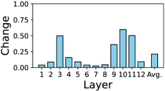
(a) +Ff
(Atb $\leftrightarrow$ AtbFf)

(b) +Res
(AtbFf $\leftrightarrow$ AtbFfRes)

(c) +Ln
(AtbFfRes $\leftrightarrow$ AtbFfResLn)

Seed 0

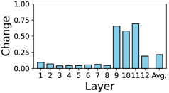
(d) +Ff
(Atb $\leftrightarrow$ AtbFf)

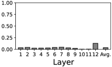
(e) +Res
(AtbFf $\leftrightarrow$ AtbFfRes)

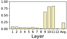
(f) +Ln
(AtbFfRes $\leftrightarrow$ AtbFfResLn)

Seed 10

(g) +Ff
(Atb $\leftrightarrow$ AtbFf)

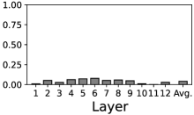
(h) +Res
(AtbFf $\leftrightarrow$ AtbFfRes)

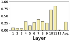
(i) +Ln
(AtbFfRes $\leftrightarrow$ AtbFfResLn)

Seed 20

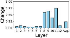
(j) +Ff
(Atb $\leftrightarrow$ AtbFf)

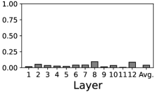
(k) +Res
(AtbFf $\leftrightarrow$ AtbFfRes)

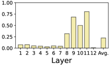
(l) +Ln
(AtbFfRes $\leftrightarrow$ AtbFfResLn)

Figure 10: Contextualization changes between before and after each component in FFBs (FF, RES2, and LN2) of four variants of BERT-base models trained with different seeds (original, 0, 10, and 20). The higher the bar, the more drastically the token-to-token contextualization (attention maps) changes due to the target component.

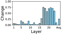
(a) +Ff
(Atb $\leftrightarrow$ AtbFf)

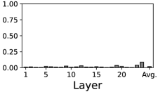
(b) +Res
(AtbFf $\leftrightarrow$ AtbFfRes)

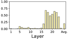
(c) +Ln
(AtbFfRes $\leftrightarrow$ AtbFfResLn)

RoBERTa-base

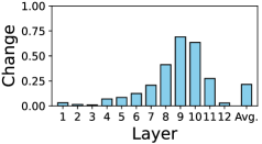
(d) +Ff
(Atb $\leftrightarrow$ AtbFf)

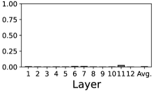
(e) +Res
(AtbFf $\leftrightarrow$ AtbFfRes)

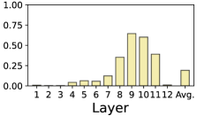
(f) +Ln
(AtbFfRes $\leftrightarrow$ AtbFfResLn)

Figure 11: Contextualization changes between before and after each component in FFBs (FF, RES2, and LN2) of two variants of RoBERTa models with different sizes (large and base). The higher the bar, the more drastically the token-to-token contextualization (attention maps) changes due to the target component.

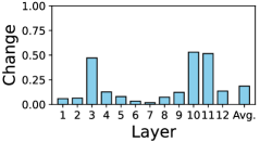
(a) +Ff
(Atb $\leftrightarrow$ AtbFf)

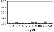
(b) +Res
(AtbFf $\leftrightarrow$ AtbFfRes)

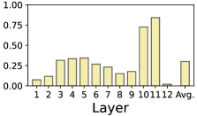
(c) +Ln
(AtbFfRes $\leftrightarrow$ AtbFfResLn)

GPT-2 (Pre-LN)

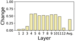
(d) +Ln
(Atb $\leftrightarrow$ AtbPreln)

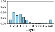
(e) +Ff
(AtbLn $\leftrightarrow$ AtbLnFf)

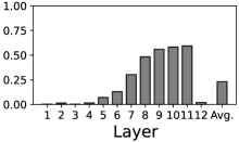
(f) +Res
(AtbLnFf $\leftrightarrow$ AtbLnFfRes)

Figure 12: Contextualization changes between before and after each component in FFBs (FF, RES2, and LN2) of BERT-base and GPT-2 on SST-2 dataset. The higher the bar, the more drastically the token-to-token contextualization (attention maps) changes due to the target component.

The contextualization changes through each component in FFBs of six variants of BERT models with different sizes are shown in Fig. 9. The results for four variants of BERT-base models trained with different seeds are shown in Fig. 10. The results for two variants of RoBERTa models with different sizes are shown in Fig. 11. The results for BERT-base and GPT-2 on the SST-2 dataset are shown in Fig. 12. These different settings with other models/datasets also yield similar results reported in § 5.1: each component did modify the input contextualization, especially in particular layers. The mask language model showed a consistent trend of larger changes by FF and LN in the mid to late layers. On the other hand, the causal language model showed a trend of larger changes by FF in the early layers.

C.2 Linguistic patterns in FF’s contextualization effects

The full lists of top 10 pairs with respect to the FF-amp score in each layer of BERT-base and GPT-2 and their token pair categories are shown in Tables 2 and 3.

Appendix D Supplemental results of dynamics of contextualization change

We reported the dynamics of contextualization change of BERT-base and GPT-2 on the Wikipedia dataset in § 6. We will report the results of the other models/datasets in this section.

D.1 Contextualization change through FF and subsequent components

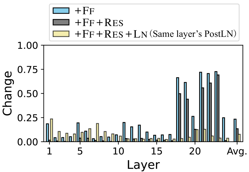
(a) BERT-large.

(b) BERT-base.

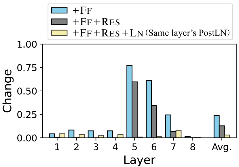
(c) BERT-medium.

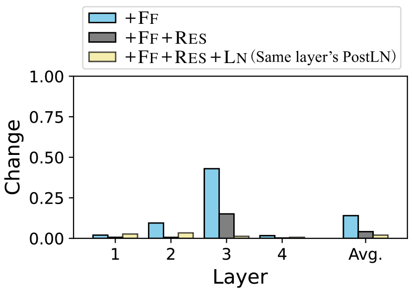
(d) BERT-small.

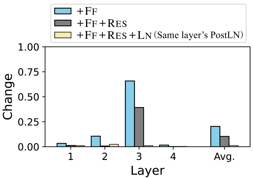
(e) BERT-mini.

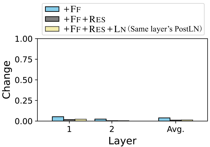
(f) BERT-tiny.

Figure 13: Contextualization changes through processing each component (FF, RES, and LN) from just before FF (ATB) in six variants of BERT models with different sizes (large, base, medium, small, mini, and tiny). The higher the bar, the more the contextualization (attention map) changes from just before FF.

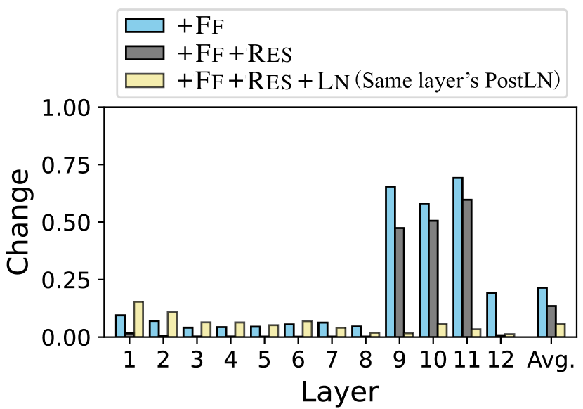
(b) BERTa-base (seed 0).

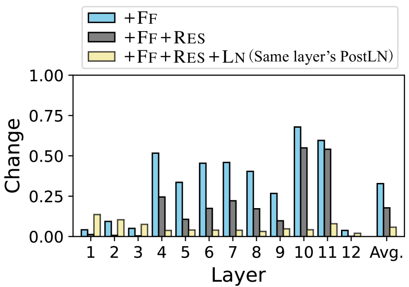
(c) BERTa-base (seed 10).

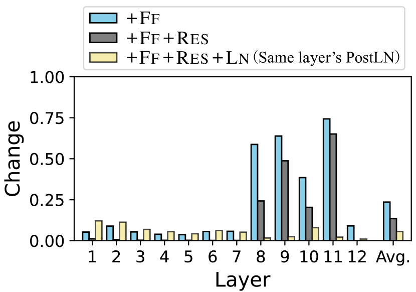
(d) BERTa-base (seed 20).

Figure 14: Contextualization changes through processing each component (FF, RES, and LN) from just before FF (ATB) in four variants of BERT-base models trained with different seeds (original, 0, 10, and 20). The higher the bar, the more the contextualization (attention map) changes from just before FF.

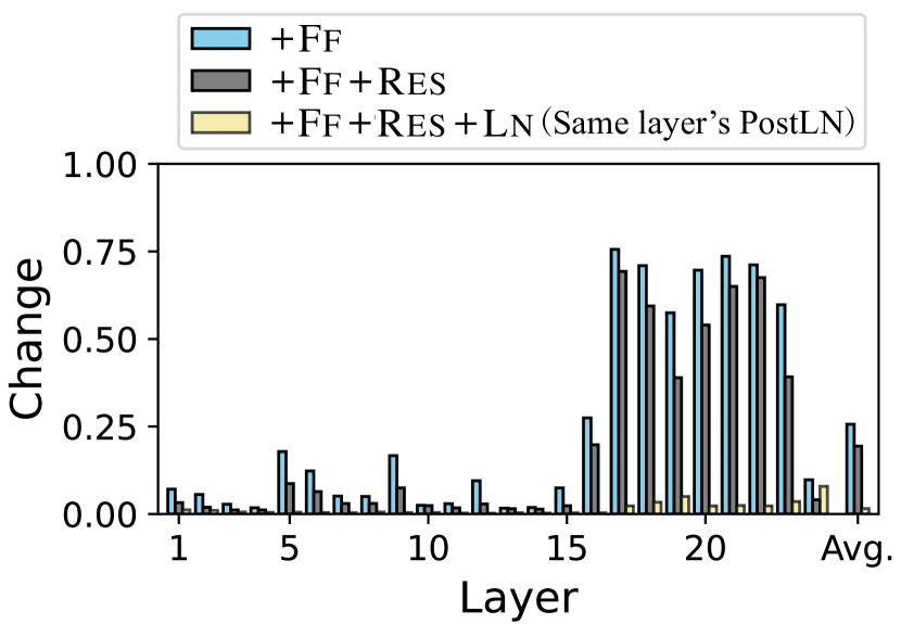
(a) RoBERTa-large.

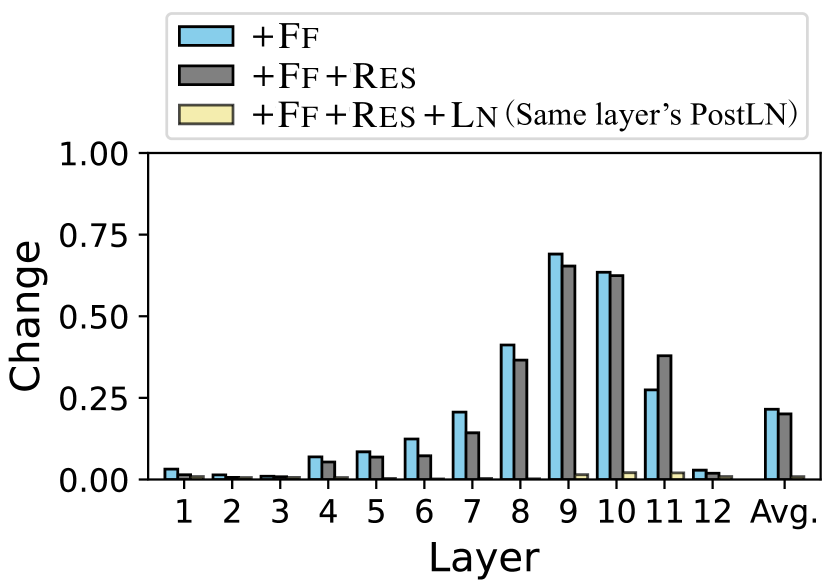
(b) RoBERTa-base.

Figure 15: Contextualization changes through processing each component (FF, RES, and LN) from just before FF (ATB) in two variants of RoBERTa models with different sizes (large and base). The higher the bar, the more the contextualization (attention map) changes from just before FF.

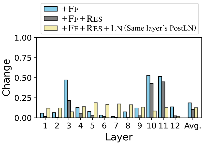
(a) BERT-base.

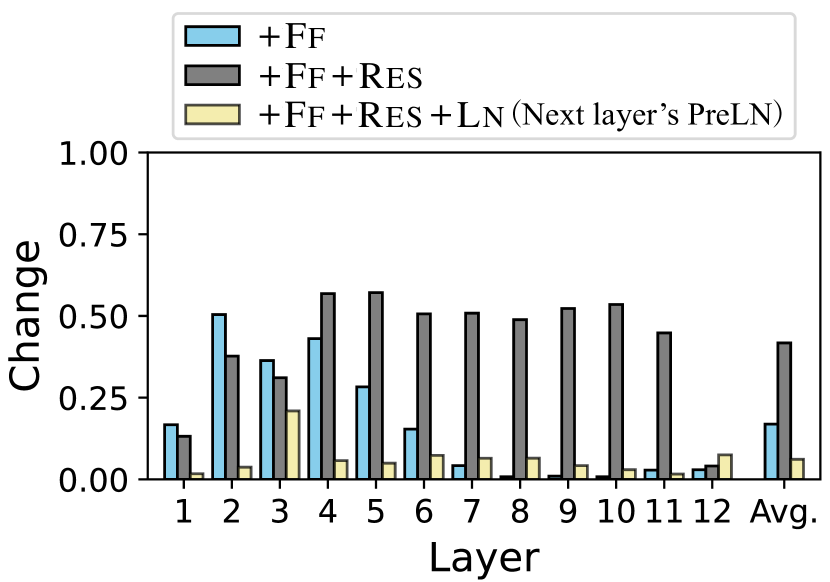
(b) GPT-2.

Figure 16: Contextualization changes through processing each component (FF, RES, and LN) from just before FF (ATB) in BERT-base and GPT-2 on SST-2 dataset. The higher the bar, the more the contextualization (attention map) changes from just before FF.

The contextualization changes through by FF and subsequent components, RES and LN, in six variants of BERT models with different sizes are shown in Fig. 13. The results for four variants of BERT-base models trained with different seeds are shown in Fig. 14. The results for two variants of RoBERTa models with different sizes are shown in Fig. 15. The results for BERT-base and GPT-2 on the SST-2 dataset are shown in Fig. 16. These different settings with other models/datasets also yield similar results reported in § 6: through the FF and subsequent RES and LN, the contextualization change score once becomes large but finally converges to be small; that is, the contextualization by FFs tends to be canceled by the following components.

D.2 FF and RES

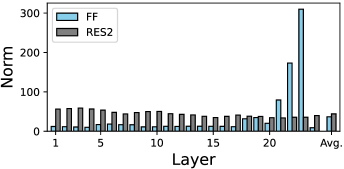
(a) BERT-large.

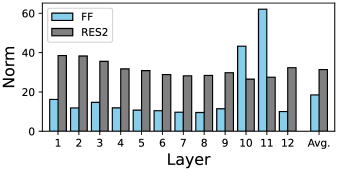
(b) BERT-base.

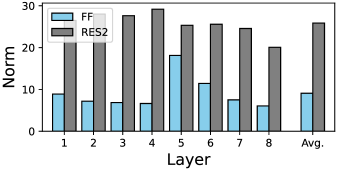
(c) BERT-medium.

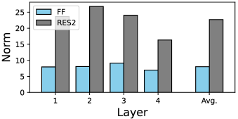
(d) BERT-small.

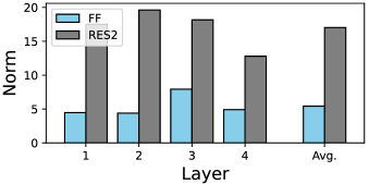
(e) BERT-mini.

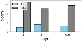
(f) BERT-tiny.

Figure 17: Averaged norm of the output vectors from FF and the bypassed vectors via RES2, calculated on the Wikipedia data for six variants of BERT models with different sizes (large, base, medium, small, mini, and tiny).

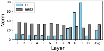
(b) BERT-base (seed 0).

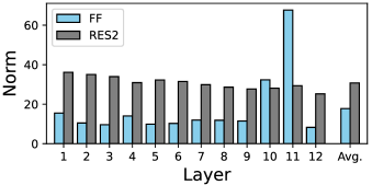
(c) BERT-base (seed 10).

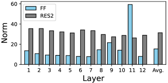
(d) BERT-base (seed 20).

Figure 18: Averaged norm of the output vectors from FF and the bypassed vectors via RES2, calculated on the Wikipedia data for four variants of BERT-base models trained with different seeds (original, 0, 10, and 20).

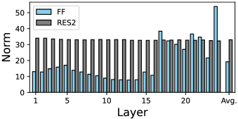
(a) RoBERTa-large.

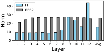
(b) RoBERTa-base.

Figure 19: Averaged norm of the output vectors from FF and the bypassed vectors via RES2, calculated on the Wikipedia data for two variants of RoBERTa models with different sizes (large and base).

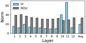
(a) RoBERTa-base.

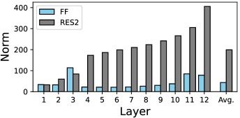
(b) GPT-2.

Figure 20: Averaged norm of the output vectors from FF and the bypassed vectors via RES2, calculated on the SST-2 dataset for BERT-base and GPT-2.

The L2 norm of the output vectors from FF and the vectors bypassed via RES2, in six variants of BERT models with different sizes are shown in Fig. 17. The results for four variants of BERT-base models trained with different seeds are shown in Fig. 18. The results for two variants of RoBERTa models with different sizes are shown in Fig. 19. The results for BERT-base and GPT-2 on the SST-2 dataset are shown in Fig. 20. These different settings with other models/datasets also yield similar results reported in § 6.1: the vectors bypassed via RES2 are more than twice as large as output vectors from FF in the L2 norm in more than half of the layers. That is, the representation (contextualization) updated by the FF tends to be overwritten/canceled by the original one.

D.3 FF and LN

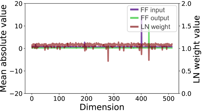
(c) $5$th layer in BERT-medium.

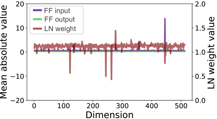
(d) $3$rd layer in BERT-small.

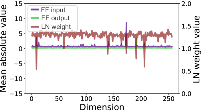
(e) $3$rd layer in BERT-mini.

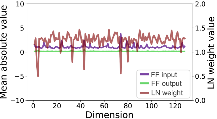
(f) $1$st layer in BERT-tiny.

Figure 21: Mean absolute value in each dimension of the input/output vectors of FF across the Wikipedia data and the LN weight values at the certain layer of six variants of BERT models with different sizes (large, base, medium, small, mini, and tiny).

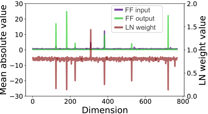
(a) $10$th layer in BERT-base (original).

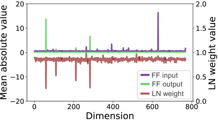
(b) $9$th layer in BERT-base (seeed 0).

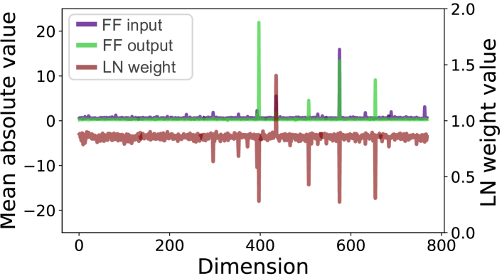
(c) $10$th layer in BERT-base (seed 10).

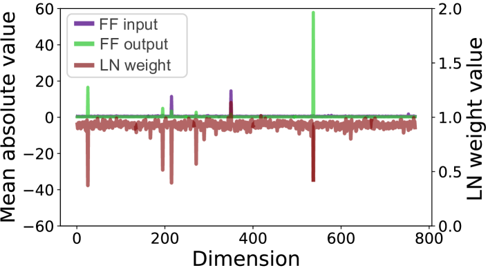
(d) $11$th layer in BERT-base (seed 20).

Figure 22: Mean absolute value in each dimension of the input/output vectors of FF across the Wikipedia data and the LN weight values at the certain layer of four variants of BERT-base models trained with different seeds (original, 0, 10, and 20).

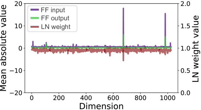
(a) $1$st layer in RoBERTa-large.

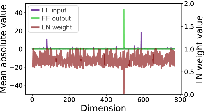
(b) $10$th layer in RoBERTa-base.

Figure 23: Mean absolute value in each dimension of the input/output vectors of FF across the Wikipedia data and the LN weight values at the certain layer of two variants of RoBERTa with different sizes (large and base).

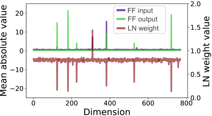
(a) $10$th layer in BERT-base.

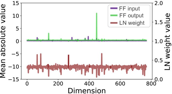
(b) $4$th layer in GPT-2.

Figure 24: Mean absolute value in each dimension of the input/output vectors of FF across the SST-2 dataset and the LN weight values at the certain layer.

Mean absolute value in each dimension of the input/output vectors of FF and the weight parameter $\bm{\gamma}$ of LN at the layer where FF’s contextualization effects are strongly cancelled by LN, in six variants of BERT models with different sizes are shown in Fig. 21. The results for four variants of BERT-base models trained with different seeds are shown in Fig. 22. The results for two variants of RoBERTa models with different sizes are shown in Fig. 23. The results for BERT-base and GPT-2 on the SST-2 dataset are shown in Fig. 24. These different settings with other models/datasets also yield similar results reported in § 6.2: the FF output representation has outliers in some specific dimensions (green lines in the figures), and the weight $\bm{\gamma}$ of LN tends to shrink these special dimensions (red lines in the figures). In the layers where FF incurs a relatively large impact on contextualization, the Pearson correlation coefficient between LN’s $\bm{\gamma}$ and mean absolute value of FF output by dimension was from $-0.38$ to $-0.93$ in BERT-large, from $-0.32$ to $-0.47$ in BERT-medium, from $-0.56$ to $-0.76$ in BERT-small, from $-0.55$ to $-0.73$ in BERT-mini, $-0.71$ in BERT-tiny, from $-0.69$ to $-0.74$ in BERT-base (seed 0), from $-0.48$ to $-0.74$ in BERT-base (seed 10), from $-0.50$ to $-0.68$ in BERT-base (seed 20). In these layers of RoBERTa models, the Pearson’s $r$ was small: from $-0.02$ to $-0.28$ in RoBERTa-large and from $0.01$ to $-0.14$ in RoBERT-base. However, the Spearman’s $\rho$ was large: from $-0.46$ to $-0.56$ in RoBERTa-large and from $0.80$ to $-0.94$ in RoBERT-base.

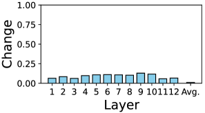
(a) Atb $\leftrightarrow$ AtbFf in BERT-base.

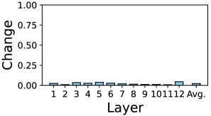
(b) AtbFf $\leftrightarrow$ AtbFfRes in GPT-2

Figure 25: Contextualization changes by FF of BERT-base and GPT-2 on Wikipedia dataset when the $1\%$ (seven) dimensions with the smallest LN weights $\bm{\gamma}$ values is ignored in the norm calculation. The higher the bar, the more drastically the token-to-token contextualization (attention maps) changes due to the target component.

In § 6.2, we also observed that ignoring such special outlier dimensions (bottom 1% with the lowest value of $\bm{\gamma}$) in calculating FF’s contextualization makes the change score quite small. The contextualization changes by FF when ignoring the dimensions are shown in Fig. 25.

BERT-large

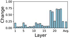
(a) +Ff
(Atb $\leftrightarrow$ AtbFf)

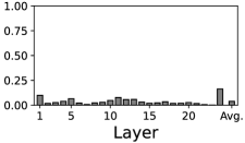
(b) +Res
(AtbFf $\leftrightarrow$ AtbFfRes)

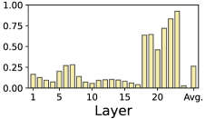
(c) +Ln
(AtbFfRes $\leftrightarrow$ AtbFfResLn)

BERT-base

(d) +Ff
(Atb $\leftrightarrow$ AtbFf)

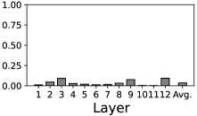
(e) +Res
(AtbFf $\leftrightarrow$ AtbFfRes)

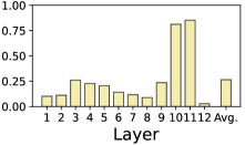
(f) +Ln
(AtbFfRes $\leftrightarrow$ AtbFfResLn)

BERT-medium

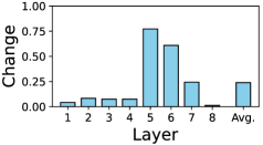
(g) +Ff
(Atb $\leftrightarrow$ AtbFf)

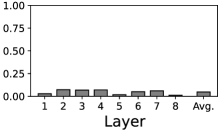
(h) +Res
(AtbFf $\leftrightarrow$ AtbFfRes)

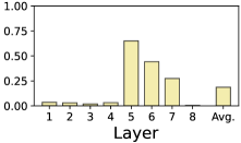
(i) +Ln
(AtbFfRes $\leftrightarrow$ AtbFfResLn)

BERT-small

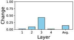
(j) +Ff
(Atb $\leftrightarrow$ AtbFf)

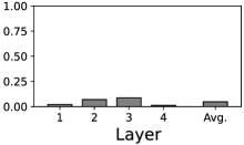
(k) +Res
(AtbFf $\leftrightarrow$ AtbFfRes)

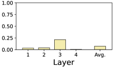
(l) +Ln
(AtbFfRes $\leftrightarrow$ AtbFfResLn)

BERT-mini

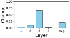
(m) +Ff
(Atb $\leftrightarrow$ AtbFf)

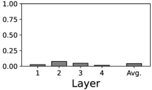
(n) +Res
(AtbFf $\leftrightarrow$ AtbFfRes)

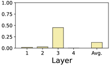
(o) +Ln
(AtbFfRes $\leftrightarrow$ AtbFfResLn)

BERT-tiny

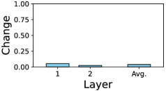
(p) +Ff
(Atb $\leftrightarrow$ AtbFf)

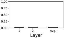
(q) +Res
(AtbFf $\leftrightarrow$ AtbFfRes)

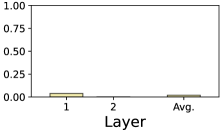
(r) +Ln
(AtbFfRes $\leftrightarrow$ AtbFfResLn)

Figure 9: Contextualization changes between before and after each component in FFBs (FF, RES2, and LN2) of six variants of BERT models with different sizes (large, base, medium, small, mini, and tiny). The higher the bar, the more drastically the token-to-token contextualization (attention maps) changes due to the target component.

Original

RoBERTa-large

BERTa-base (Post-LN)

(a) BERTa-base (original).

Table 2: Word pairs for which FF amplified the interaction the most in BERT. The text colors are aligned with word pair categories: subword, compound noun, common expression, same token, named entity, and others.

Layer	Top amplified token-pairs
1	(##our, det), (##iques, ##mun), (##cend, trans), (outer, space), (##ili, res),
	(##ific, honor), (##nate, ##imi), (opera, soap), (deco, art), (##night, week)
2	(##roy, con), (guard, national), (america, latin), (easily, could), (##oy, f),
	(marshall, islands), (##ite, rec), (channel, english), (finance, finance), (##ert, rev)
3	(’, t), (##mel, ##ons), (hut, ##chin), (water, ##man), (paso, ##k),
	(avoid, ##ant), (toys, ##hop), (competitive, ##ness), (##la, ##p), (##tree, ##t)
4	(##l, ds), (##l, ##tera), (##cz, ##ave), (##r, ##lea), (##e, beth),
	(##ent, ##ili), (##er, ##burn), (##et, mn), (##ve, wai), (##rana, ke)
5	(##ent, ##ili), (##ious, ##car), (##on, ##ath), (##l, ds), (##r, ##ense),
	(##ence, ##ili), (res, ##ili), (##rative, ##jo), (##ci, ##pres), (##able, ##vor)
6	(on, clay), (with, charged), (##ci, ##pres), (be, considers), (on, behalf),
	(fleming, colin), (##r, ##lea), (-, clock), (##ur, nam), (by, denoted)
7	(##ons, ##mel), (vi, saint), (vi, st), (##l, ##ife), (##ti, jon),
	(##i, wii), (##en, ##chel), (##son, bis), (vessels, among), (##her, ##rn)
8	(##ano, ##lz), (bo, ##lz), (nathan, or), (arabia, against), (sant, ##ini),
	(previous, unlike), (saudi, against), (##ia, ##uring), (he, gave), (tnt, equivalent)
9	(no, situation), (##ek, czech), (according, situation), (decided, year), (v, classification),
	(eventually, year), (but, difficulty), (##ference, track), (she, teacher), (might, concerned)
10	(jan, ##nen), (hee, ##mjㅓ), (primary, stellar), (crete, crete), (nuclear, 1991),
	(inspector, police), (##tu, ##nen), (quote, quote), (f, stellar), (v, stellar)
11	(tiny, tiny), (##water, ##water), (hem, hem), (suddenly, suddenly), (fine, singer),
	(henley, henley), (highway, highway), (moving, moving), (dug, dug), (farmers, agricultural)
12	(luis, luis), (tong, 同), (board, judicial), (##i, index), (—, —),
	(four, fifty), (cloud, thunder), (located, transmitter), (##ota, ##ɔ), (##ss, analysis)

Table 3: Word pairs for which FF amplified the interaction the most in GPT-2. The text colors are aligned with word pair categories: subword, compound noun, common expression, same token, named entity, and others.

Layer	Top amplified token-pairs
1	(ies, stud), (ning, begin), (ever, how), (ents, stud), (ited, rec),
	(une, j), (al, sever), (itions, cond), (ang, p), (ree, c)
2	(al, sever), (itions, cond), (z, jan), (ning, begin), (_was, this),
	(er, care), (ies, stud), (une, j), (s, 1990), (ents, stud)
3	(_than, _rather), (z, jan), (_then, since), (bin, ro), (_long, _how),
	(ting, _rever), (une, j), (_others, _among), (arks, _cl), (_into, _turning)
4	(_same, _multiple), (ouri, _miss), (_jung, lex), (_b, _strength), (_others, _among),
	(_based, _”.), (adesh, hra), (_top, _among), (t, _give), (bin, ro)
5	(ol, _brist), (ol, ink), (gal, _man), (ac, _pens), (op, _link),
	(_whit, _&), (ant, _avoid), (_people, _important), (un, _bra), (_1995, _1994)
6	(ol, ink), (_del, del), (o, _dec), (ist, oh), (it, _me),
	(_route, route), (thel, in), (ord, m), (adier, division), (we, ob)
7	(_ve, _las), (che, _ro), (43, _âĢĵ), (_green, _mark), (_cer, _family),
	(_jack, eter), (orses, ’), (_kilometres, _lies), (,, _disappointed), (umer, in)
8	(_ar, _goddess), (_d, ight), (_33, _density), (_cer, _family), (_08, _2007),
	(bid, _family), (_14, _density), (_e, _family), (_50, _yield), (_15, _density)
9	(_ray, _french), (_11, uly), (_one, _score), (on, _french), (_41, _%),
	(_37, _%), (_equipped, _another), (bc, _;), (ad, en), (.,, te)
10	(ho, ind), (_by, ashi), (_bra, _von), (_and, _317), (ad, en),
	(_loves, ashi), (_u, asaki), (_he, ner), (_land, ines), (_de, die)
11	(it, ’), (uman, _when), (ave, _daughters), (_bird, _:), (ic, there),
	(ia, _counties), (bc, _;), (_and, had), (_2010, _us), (ĩ, :)
12	(_operational, _not), (_answered, _therefore), (_degrees, _having), (_varying, _having),
	(k, rant), (_supplied, _also), (_daring, _has), (_prominent, ’s), (a, ually), (_stress, _:)

(a) BERT-base (original).

(a) $18$th layer in BERT-large.

(b) $10$th layer in BERT-base.

References

- Abnar & Zuidema (2020) Samira Abnar and Willem Zuidema. Quantifying Attention Flow in Transformers. In Proceedings of the 58th Annual Meeting of the Association for Computational Linguistics (ACL), pp. 4190–4197, 2020. doi: 10.18653/v1/2020.acl-main.385. URL https://www.aclweb.org/anthology/2020.acl-main.385.
- Braşoveanu & Andonie (2020) Adrian M. P. Braşoveanu and Răzvan Andonie. Visualizing Transformers for NLP: A Brief Survey. In 24th International Conference Information Visualisation (IV), pp. 270–279, 2020. doi: 10.1109/IV51561.2020.00051. URL https://ieeexplore.ieee.org/abstract/document/9373074.
- Brown et al. (2020) Tom Brown, Benjamin Mann, Nick Ryder, Melanie Subbiah, Jared D Kaplan, Prafulla Dhariwal, Arvind Neelakantan, Pranav Shyam, Girish Sastry, Amanda Askell, Sandhini Agarwal, Ariel Herbert-Voss, Gretchen Krueger, Tom Henighan, Rewon Child, Aditya Ramesh, Daniel Ziegler, Jeffrey Wu, Clemens Winter, Chris Hesse, Mark Chen, Eric Sigler, Mateusz Litwin, Scott Gray, Benjamin Chess, Jack Clark, Christopher Berner, Sam McCandlish, Alec Radford, Ilya Sutskever, and Dario Amodei. Language Models are Few-Shot Learners. In Advances in Neural Information Processing Systems 33 (NeurIPS), volume 33, pp. 1877–1901, 2020. URL https://proceedings.neurips.cc/paper/2020/file/1457c0d6bfcb4967418bfb8ac142f64a-Paper.pdf.
- Brunner et al. (2020) Gino Brunner, Yang Liu, Damián Pascual, Oliver Richter, Massimiliano Ciaramita, and Roger Wattenhofer. On Identifiability in Transformers. In 8th International Conference on Learning Representations (ICLR), 2020. URL https://openreview.net/forum?id=BJg1f6EFDB.
- Burkart & Huber (2021) Nadia Burkart and Marco F Huber. A Survey on the Explainability of Supervised Machine Learning. Artificial Intelligence Research, 70:245–317, 2021. doi: 10.1613/jair.1.12228.
- Carvalho et al. (2019) Diogo V Carvalho, Eduardo M Pereira, and Jaime S Cardoso. Machine Learning Interpretability: A Survey on Methods and Metrics. Electronics, 8(8), 832, 2019. ISSN 2079-9292. doi: 10.3390/electronics8080832. URL https://www.mdpi.com/2079-9292/8/8/832.
- Clark et al. (2019) Kevin Clark, Urvashi Khandelwal, Omer Levy, and Christopher D Manning. What Does BERT Look At? An Analysis of BERT’s Attention. In Proceedings of the 2019 ACL Workshop BlackboxNLP: Analyzing and Interpreting Neural Networks for NLP, pp. 276–286, 2019. doi: 10.18653/v1/W19-4828. URL https://www.aclweb.org/anthology/W19-4828.
- Dai et al. (2022) Damai Dai, Li Dong, Yaru Hao, Zhifang Sui, Baobao Chang, and Furu Wei. Knowledge Neurons in Pretrained Transformers. In Proceedings of the 60th Annual Meeting of the Association for Computational Linguistics (ACL), pp. 8493–8502, 2022. doi: 10.18653/v1/2022.acl-long.581. URL https://aclanthology.org/2022.acl-long.581.
- Devlin et al. (2019) Jacob Devlin, Ming-Wei Chang, Kenton Lee, and Kristina Toutanova. BERT: Pre-training of Deep Bidirectional Transformers for Language Understanding. In Proceedings of the 2019 Conference of the North American Chapter of the Association for Computational Linguistics: Human Language Technologies (NAACL-HLT), pp. 4171–4186, 2019. doi: 10.18653/v1/N19-1423. URL https://www.aclweb.org/anthology/N19-1423/.
- Elfwing et al. (2018) Stefan Elfwing, Eiji Uchibe, and Kenji Doya. Sigmoid-weighted linear units for neural network function approximation in reinforcement learning. Neural Networks, 107:3–11, 2018. ISSN 0893-6080. doi: 10.1016/j.neunet.2017.12.012. URL https://www.sciencedirect.com/science/article/pii/S0893608017302976. Special issue on deep reinforcement learning.
- Geva et al. (2021) Mor Geva, Roei Schuster, Jonathan Berant, and Omer Levy. Transformer Feed-Forward Layers Are Key-Value Memories. In Proceedings of the 2021 Conference on Empirical Methods in Natural Language Processing (EMNLP), pp. 5484–5495, 2021. doi: 10.18653/v1/2021.emnlp-main.446. URL https://aclanthology.org/2021.emnlp-main.446.
- Hendrycks & Gimpel (2016) Dan Hendrycks and Kevin Gimpel. Gaussian Error Linear Units (GELUs). arXiv preprint, cs.LG/1606.08415v4, 2016. doi: 10.48550/arXiv.1606.08415.
- Houlsby et al. (2019) Neil Houlsby, Andrei Giurgiu, Stanislaw Jastrzebski, Bruna Morrone, Quentin De Laroussilhe, Andrea Gesmundo, Mona Attariyan, and Sylvain Gelly. Parameter-Efficient transfer learning for NLP. In Kamalika Chaudhuri and Ruslan Salakhutdinov (eds.), Proceedings of the 36th International Conference on Machine Learning, volume 97 of Proceedings of Machine Learning Research, pp. 2790–2799. PMLR, 2019.
- Kobayashi et al. (2020) Goro Kobayashi, Tatsuki Kuribayashi, Sho Yokoi, and Kentaro Inui. Attention is Not Only a Weight: Analyzing Transformers with Vector Norms. In Proceedings of the 2020 Conference on Empirical Methods in Natural Language Processing (EMNLP), pp. 7057–7075, 2020. doi: 10.18653/v1/2020.emnlp-main.574. URL https://www.aclweb.org/anthology/2020.emnlp-main.574.
- Kobayashi et al. (2021) Goro Kobayashi, Tatsuki Kuribayashi, Sho Yokoi, and Kentaro Inui. Incorporating Residual and Normalization Layers into Analysis of Masked Language Models. In Proceedings of the 2021 Conference on Empirical Methods in Natural Language Processing (EMNLP), pp. 4547–4568, 2021. doi: 10.18653/v1/2021.emnlp-main.373. URL https://aclanthology.org/2021.emnlp-main.373.
- Kovaleva et al. (2019) Olga Kovaleva, Alexey Romanov, Anna Rogers, and Anna Rumshisky. Revealing the Dark Secrets of BERT. In Proceedings of the 2019 Conference on Empirical Methods in Natural Language Processing and the 9th International Joint Conference on Natural Language Processing (EMNLP-IJCNLP), pp. 4364–4373, 2019. doi: 10.18653/v1/D19-1445. URL https://www.aclweb.org/anthology/D19-1445.
- Kriegeskorte et al. (2008) Nikolaus Kriegeskorte, Marieke Mur, and Peter Bandettini. Representational similarity analysis - connecting the branches of systems neuroscience. Frontiers in Systems Neuroscience, 2:4, 2008. doi: 10.3389/neuro.06.004.2008. URL https://www.frontiersin.org/article/10.3389/neuro.06.004.2008.
- Liu et al. (2019) Yinhan Liu, Myle Ott, Naman Goyal, Jingfei Du, Mandar Joshi, Danqi Chen, Omer Levy, Mike Lewis, Luke Zettlemoyer, and Veselin Stoyanov. RoBERTa: A Robustly Optimized BERT Pretraining Approach. arXiv preprint, cs.CL/1907.11692v1, 2019. doi: 10.48550/arXiv.1907.11692. URL http://arxiv.org/abs/1907.11692v1.
- Lloyd S. (1953) Shapley Lloyd S. A Value for n-person Games. Contributions to the Theory of Games (AM-28), Volume II, pp. 307–318, 1953. doi: 10.1515/9781400881970-018. URL https://www.jstor.org/stable/j.ctt1b9x1zv.24.
- Modarressi et al. (2022) Ali Modarressi, Mohsen Fayyaz, Yadollah Yaghoobzadeh, and Mohammad Taher Pilehvar. GlobEnc: Quantifying Global Token Attribution by Incorporating the Whole Encoder Layer in Transformers. In Proceedings of the 2022 Conference of the North American Chapter of the Association for Computational Linguistics: Human Language Technologies (NAACL-HLT), pp. 258–271, 2022. doi: 10.18653/v1/2022.naacl-main.19. URL https://aclanthology.org/2022.naacl-main.19.
- Modarressi et al. (2023) Ali Modarressi, Mohsen Fayyaz, Ehsan Aghazadeh, Yadollah Yaghoobzadeh, and Mohammad Taher Pilehvar. DecompX: Explaining Transformers Decisions by Propagating Token Decomposition. In Proceedings of the 61st Annual Meeting of the Association for Computational Linguistics (ACL), pp. 2649–2664, 2023. doi: 10.18653/v1/2023.acl-long.149. URL https://aclanthology.org/2023.acl-long.149.
- Nair & Hinton (2010) Vinod Nair and Geoffrey E. Hinton. Rectified Linear Units Improve Restricted Boltzmann Machines. In Proceedings of the 27th International Conference on Machine Learning (ICML), pp. 807–814, 2010. URL https://icml.cc/Conferences/2010/papers/432.pdf.
- Oba et al. (2021) Daisuke Oba, Naoki Yoshinaga, and Masashi Toyoda. Exploratory Model Analysis Using Data-Driven Neuron Representations. In Proceedings of the Fourth BlackboxNLP Workshop on Analyzing and Interpreting Neural Networks for NLP, pp. 518–528, 2021. doi: 10.18653/v1/2021.blackboxnlp-1.41. URL https://aclanthology.org/2021.blackboxnlp-1.41.
- Radford et al. (2019) Alec Radford, Jeffrey Wu, Rewon Child, David Luan, Dario Amodei, and Ilya Sutskever. Language Models are Unsupervised Multitask Learners. Technical report, OpenAI, 2019. URL https://d4mucfpksywv.cloudfront.net/better-language-models/language-models.pdf.
- Rogers et al. (2020) Anna Rogers, Olga Kovaleva, and Anna Rumshisky. A Primer in BERTology: What We Know About How BERT Works. Transactions of the Association for Computational Linguistics (TACL), 8:842–866, 2020. doi: 10.1162/tacl˙a˙00349. URL https://www.aclweb.org/anthology/2020.tacl-1.54.
- Sellam et al. (2022) Thibault Sellam, Steve Yadlowsky, Ian Tenney, Jason Wei, Naomi Saphra, Alexander D’Amour, Tal Linzen, Jasmijn Bastings, Iulia Raluca Turc, Jacob Eisenstein, Dipanjan Das, and Ellie Pavlick. The MultiBERTs: BERT Reproductions for Robustness Analysis. In 10th International Conference on Learning Representations (ICLR), 2022. URL https://openreview.net/forum?id=K0E_F0gFDgA.
- Socher et al. (2013) Richard Socher, Alex Perelygin, Jean Wu, Jason Chuang, Christopher D. Manning, Andrew Ng, and Christopher Potts. Recursive Deep Models for Semantic Compositionality Over a Sentiment Treebank. In Proceedings of the 2013 Conference on Empirical Methods in Natural Language Processing (EMNLP), pp. 1631–1642, 2013. URL https://www.aclweb.org/anthology/D13-1170.
- Sundararajan et al. (2017) Mukund Sundararajan, Ankur Taly, and Qiqi Yan. Axiomatic Attribution for Deep Networks. In Proceedings of the 34th International Conference on Machine Learning (ICML), PMLR, volume 70, pp. 3319–3328, 2017. URL https://proceedings.mlr.press/v70/sundararajan17a.html.
- Tenney et al. (2019) Ian Tenney, Dipanjan Das, and Ellie Pavlick. BERT Rediscovers the Classical NLP Pipeline. In Proceedings of the 57th Annual Meeting of the Association for Computational Linguistics (ACL), pp. 4593–4601, 2019. doi: 10.18653/v1/P19-1452. URL https://www.aclweb.org/anthology/P19-1452/.
- Tolstikhin et al. (2021) Ilya O Tolstikhin, Neil Houlsby, Alexander Kolesnikov, Lucas Beyer, Xiaohua Zhai, Thomas Unterthiner, Jessica Yung, Andreas Steiner, Daniel Keysers, Jakob Uszkoreit, et al. Mlp-mixer: An all-mlp architecture for vision. Advances in neural information processing systems, 34:24261–24272, 2021.
- Touvron et al. (2023a) Hugo Touvron, Thibaut Lavril, Gautier Izacard, Xavier Martinet, Marie-Anne Lachaux, Timothée Lacroix, Baptiste Rozière, Naman Goyal, Eric Hambro, Faisal Azhar, Aurelien Rodriguez, Armand Joulin, Edouard Grave, and Guillaume Lample. Llama: Open and efficient foundation language models, 2023a. URL https://arxiv.org/abs/2302.13971v1.
- Touvron et al. (2023b) Hugo Touvron, Louis Martin, Kevin Stone, Peter Albert, Amjad Almahairi, Yasmine Babaei, Nikolay Bashlykov, Soumya Batra, Prajjwal Bhargava, Shruti Bhosale, Dan Bikel, Lukas Blecher, Cristian Canton Ferrer, Moya Chen, Guillem Cucurull, David Esiobu, Jude Fernandes, Jeremy Fu, Wenyin Fu, Brian Fuller, Cynthia Gao, Vedanuj Goswami, Naman Goyal, Anthony Hartshorn, Saghar Hosseini, Rui Hou, Hakan Inan, Marcin Kardas, Viktor Kerkez, Madian Khabsa, Isabel Kloumann, Artem Korenev, Punit Singh Koura, Marie-Anne Lachaux, Thibaut Lavril, Jenya Lee, Diana Liskovich, Yinghai Lu, Yuning Mao, Xavier Martinet, Todor Mihaylov, Pushkar Mishra, Igor Molybog, Yixin Nie, Andrew Poulton, Jeremy Reizenstein, Rashi Rungta, Kalyan Saladi, Alan Schelten, Ruan Silva, Eric Michael Smith, Ranjan Subramanian, Xiaoqing Ellen Tan, Binh Tang, Ross Taylor, Adina Williams, Jian Xiang Kuan, Puxin Xu, Zheng Yan, Iliyan Zarov, Yuchen Zhang, Angela Fan, Melanie Kambadur, Sharan Narang, Aurelien Rodriguez, Robert Stojnic, Sergey Edunov, and Thomas Scialom. Llama 2: Open Foundation and Fine-Tuned Chat Models, 2023b. URL https://arxiv.org/abs/2307.09288v2.
- Turc et al. (2019) Iulia Turc, Ming-Wei Chang, Kenton Lee, and Kristina Toutanova. Well-Read Students Learn Better: On the Importance of Pre-training Compact Models. arXiv preprint, cs.CL/1908.08962v2, 2019. doi: 10.48550/arXiv.1908.08962. URL https://arxiv.org/abs/1908.08962v2.
- Vaswani et al. (2017) Ashish Vaswani, Noam Shazeer, Niki Parmar, Jakob Uszkoreit, Llion Jones, Aidan N Gomez, Lukasz Kaiser, and Illia Polosukhin. Attention is All you Need. In Advances in Neural Information Processing Systems 30 (NIPS), pp. 5998–6008, 2017. URL http://papers.nips.cc/paper/7181-attention-is-all-you-need.
- Vig (2019) Jesse Vig. Visualizing Attention in Transformer-Based Language Representation Models. arXiv preprint arXiv:1904.02679, 2019. URL https://arxiv.org/abs/1904.02679v2.
- Xiong et al. (2020) Ruibin Xiong, Yunchang Yang, Di He, Kai Zheng, Shuxin Zheng, Chen Xing, Huishuai Zhang, Yanyan Lan, Liwei Wang, and Tieyan Liu. On Layer Normalization in the Transformer Architecture. In Proceedings of the 37th International Conference on Machine Learning (ICML), PMLR, volume 119, pp. 10524–10533, 2020. URL https://proceedings.mlr.press/v119/xiong20b.html.
- Zhang et al. (2022) Susan Zhang, Stephen Roller, Naman Goyal, Mikel Artetxe, Moya Chen, Shuohui Chen, Christopher Dewan, Mona Diab, Xian Li, Xi Victoria Lin, Todor Mihaylov, Myle Ott, Sam Shleifer, Kurt Shuster, Daniel Simig, Punit Singh Koura, Anjali Sridhar, Tianlu Wang, and Luke Zettlemoyer. OPT: Open Pre-trained Transformer Language Models. arXiv preprint, cs.CL/2205.01068v4, 2022. URL https://arxiv.org/abs/2205.01068v4.