Structure and Kinematics of Sh2-138 - A distant hub-filament system in the outer Galactic plane

Abstract

We present a molecular line study of the Sh2-138 (IRAS 22308+5812) “hub-filament” system with an aim to investigate its structure and kinematics. Archival CO molecular line data from the Canadian Galactic Plane Survey (CO(J=1–0)) for the wider region ($\sim$ 50′$\times$50′) and the James Clerk Maxwell Telescope (CO(3-2), ¹³CO(3-2), and C¹⁸O(3-2)) for the central portion ($\sim$ 5′$\times$5′) have been utilised. Analysis of the CO(1-0) spectra for the extended region in conjunction with the hub and filament identification using column density map and the getsf tool, respectively, reveals a complex structure with the spectral extraction for the central position displaying multiple velocity components. Based on the Herschel 70 µm  warm dust emission, one of the filaments in the extended region was inferred to be associated with active star formation, and is host to a Bolocam 1.1 mm clump of $\sim$ 1606 M_☉. Integrated intensity map of ¹³CO(3-2)  emission, constructed from clumps detected at above 5$\sigma$ in position-position-velocity space, reveals three filamentary structures (labelled W-f, SW-f, and SE-f) in the central portion. Velocity gradients observed in ¹³CO(3-2)  position-velocity slices point to longitudinal gas flow along the filaments into the central region. Filaments W-f, SW-f, and SE-f were calculated to have observed line masses of $\sim$ 32, 33.5, and 50 M_☉ pc^-1, respectively. The cloud was found to be dominated by supersonic and non-thermal motions, with high Mach numbers ($\gtrsim$ 3) and low thermal to non-thermal pressure ratio ($\sim$ 0.01–0.1).

1 Introduction

Understanding the evolutionary sequence of high-mass stars ($\geq$8 M_☉) is an area of ongoing development in astronomy (Zinnecker & Yorke, 2007). Observations indicate that massive stars are generally found in the center of embedded young stellar clusters in giant molecular clouds (Kumar et al., 2006; Beuther et al., 2007; Portegies Zwart et al., 2010). The Lyman continuum radiation output of such stars ionizes the natal cloud leading to the formation of H II regions, which evolve from a compact to classical phase. Observations in the past few decades have led to an empirical view that, for high-mass stars, dense and massive cold cloud structures could be analogous to prestellar cores in low-mass stars (Motte et al., 2018). Infrared dark clouds – seen in absorption against mid-infrared emission (such as Spitzer) – are promising sites of such dense cloud cores, with some resembling the “hub-filament” model of Myers (2009) seen in emission in far-infrared observations by Herschel. According to Inutsuka & Miyama (1997), filamentary features represent an important step in the evolutionary life of a molecular cloud as it progresses towards fragmenting into dense clumps. The study by Kumar et al. (2020) has even concluded that almost all massive star formation occurs in the hubs and suggested a “filaments to clusters” paradigm.

It thus becomes an imperative to study young stellar clusters hosting high-mass stars, with the presence of photodissociated region being their typical signature. Sh2-138 (or G105.6270+00.3388; l $\sim$ 105.6270°, b $\sim$ +0.3392°), associated with the IRAS source (IRAS 22308+5812) in Cepheus, is one such Galactic optical H II region. The extent of the ionized region and the parameters derived (electron density, emission measure, etc) from radio continuum observations (Fich, 1993; Martín-Hernández et al., 2002) showed it to be a classical H II region (Kurtz, 2002). Early optical and near-infrared observations by Deharveng et al. (1999) had found four O/B-type stars in a similar layout as the Orion Trapezium cluster. The multiwavelength study of Baug et al. (2015) revealed further compact radio clumps, as well as provided age and spectral type estimates of the cluster of O/B stars. Their analyses found an isolated cluster of young stellar objects – with a mean age of $\sim$ 1 Myr – centered on the location of the IRAS source lying at the junction of filaments. The massive star(s) seem to be driving molecular outflows in the region (Qin et al., 2008), and a possible (weak) water maser detection (Cesaroni et al., 1988; Palagi et al., 1993; Wouterloot et al., 1993) is likely an outcome of this (Fish, 2007), though more recent studies (Urquhart et al., 2011) suggest non-detection. It should however be noted that there is an absence of methanol masers in the region (Slysh et al., 1999; Szymczak et al., 2000). Early molecular observations of the region in CO (Dickinson et al., 1974; Blitz et al., 1982; Wouterloot & Brand, 1989), HCN (Burov et al., 1988), HCO+ (Zinchenko et al., 1990; Yoo et al., 2018), NH₃ (Harju et al., 1993; Urquhart et al., 2011), CS (Bronfman et al., 1996), and other species’ isotopologues (Johansson et al., 1994) were able to detect the spectra of the molecular cloud centered in the $\sim$-53 to -52 km s^-1  range. More recent higher resolution CO observations (Kerton & Brunt, 2003; Brunt et al., 2003) have found multiple velocity components associated with the molecular cloud. The multitude of molecular line studies have probed different physical conditions in the cloud, but at specific locations (mostly on the coordinate of the IRAS source) and have not looked at the spatial variation of the spectra (and thus the physical conditions) in the wider region, though this could be partly due to the low resolution of some of the studies. The relatively comprehensive study of Baug et al. (2015) has focussed on optical and near-infrared study of stellar sources and the ionized morphology. Also, their inference from Herschel column density map that this region lies at the junction of filaments makes it but natural to explore the structure of the filamentary features in molecular line transitions. The current paper aims to fulfill this void (partly, in various transitions of CO isotopologues) for a better understanding of the interplay of (massive) stellar cluster and hub-filament system (HFS) in the Sh2-138 H II region.

Deharveng et al. (1999) use a distance of 5.0 $\pm$ 1.0 kpc for the Sh2-138 H II region in their analysis based on the average distance to nearby compact H II regions, though their kinematic distance calculation from V${}_{\textsc{lsr}}$(CO) suggests a value in the range 5.45-5.9 kpc. Anderson et al. (2014) also calculated a value of $\sim$5.8 kpc based on the velocity from NH₃ spectrum. According to Blitz et al. (1982), H II regions with similar velocities ($\sim$-53 km s^-1) near Sh2-138, namely Sh2-148 and Sh2-149, have distances of $\sim$5.5 and 5.4 kpc, respectively. Similar distance estimates have been used by Wouterloot & Brand (1989, $\sim$ 5.7 kpc); Johansson et al. (1994, $\sim$ 6.0 kpc) using a mean of kinematic distance and the estimate from the size-linewidth relation; Martín-Hernández et al. (2002, $\sim$ 5.5 kpc); Baug et al. (2015, $\sim$ 5.7 kpc); and Zhang et al. (2020, $\sim$ 5.7 kpc). For the purpose of this paper, we thus adopt the distance of 5.7 kpc of Baug et al. (2015).

The organisation of the paper is as follows. In section 2, we list the various datasets used in this paper. This is followed by analysis and results in section 3, where the large scale view of the region is examined (section 3.1) and the kinematics of the molecular gas in the central region is presented (section 3.2) A discussion of our results follows in section 4 and finally we conclude with a summary of major findings in section 5.

2 Data Used

Table 1 provides a summary of datasets used in this paper. A brief description of the salient portions is being provided in the following part of this section.

Archival spectral cubes for ¹²CO(1-0) (2.6 mm) emission produced by the Canadian Galactic Plane Survey (CGPS) Consortium (Taylor et al., 2003) were procured for the region. The CGPS cubes are based on the Five College Radio Astronomy Observatory (FCRAO) outer Galaxy survey (Heyer et al., 1998) regridded to a pixel scale of 18″  and channel width of 0.824 km s^-1. The spectral cube data, given in radiation temperature scale (i.e. T${}_{\textsc{r}}^{*}$), has a spatial resolution of 100.44″.

Besides CGPS, archival JCMT (James Clerk Maxwell Telescope) observations of the Sh2-138 (G105.6270+00.3388) region were downloaded using the CADC data repository. Calibrated spectral cubes for the three molecular lines – CO(3-2)(rest frequency = 345.79599 GHz; Proposal ID : M07AU08; Int. time : 17.983 s), ¹³CO(3-2)(rest frequency = 330.587960 GHz; Proposal ID : M08BU18; Int. time : 48.896 s), and C¹⁸O(3-2)(rest frequency = 329.330545 GHz; Proposal ID : M08BU18; Int. time : 48.808 s) – observed using the HARP/ACSIS (Heterodyne Array Receiver Programme/Auto-Correlation Spectral Imaging System; Buckle et al., 2009) spectral imaging system were retrieved. The J=3–2 transition traces gas at a higher critical density (Buckle et al., 2010, $\sim$ 10^4-5 cm^-3) than the CGPS CO(J=1–0) data whose critical density is of the order of $\sim$ 10³ cm^-3 (Bolatto et al., 2013; Shirley, 2015). The temperature scale used for the pixel brightness units is T${}_{\textsc{a}}^{*}$ (antenna temperature) for all the three spectral cubes. Basic processing for the purpose of our analysis involved conversion of spectral axis units from frequency to velocity scale, and the coordinate system to Galactic from FK5. Both the ¹³CO(3-2)  and C¹⁸O(3-2)  JCMT cubes had a channel width of $\sim$ 0.05 km s^-1, with the mean rms noise being $\sim$ 0.96$\pm$0.45 K and 1.3$\pm$0.7 K, respectively. While we use these cubes for spectra analysis due to their high velocity resolution; for the detection of spatial structures, we averaged and rebinned both these cubes along the spectral axis to 0.5 km s^-1  channels. The resultant rebinned cubes had a reduced mean rms noise of 0.30$\pm$0.14 K and 0.41$\pm$0.23 K for ¹³CO(3-2)  and C¹⁸O(3-2), respectively. The above tasks were implemented using the starlink kappa (Currie et al., 2014) package commands such as “wcsattrib” and “sqorst”. The CO(3-2)  cube – which had a native channel width of $\sim$0.42 km s^-1  and a mean rms noise of 0.53$\pm$0.2 K – was mainly used to examine the morphology of the region. Each of the images in the cubes has a pixel scale of $\sim$7.3″, and a beamsize of $\sim$14″  (Buckle et al., 2009, 2010; Davis et al., 2010; Graves et al., 2010) which is equivalent to $\sim$0.4 pc at a distance of 5.7 kpc.

For the purpose of examining the column density and temperature of the region, we retrieved the publicly available Vialactea Herschel column density and temperature maps for the same (Molinari et al., 2010). These maps have been generated by applying the Bayesian point-process procedure (Marsh et al., 2015) to Hi-Gal survey images (Marsh et al., 2017). The pixel scale of $\sim$6″  and a resolution of $\sim$12″  makes them suitable to examine in conjunction with the JCMT data. Finally, Herschel PACS (Photodetector Array Camera and Spectrometer; Poglitsch et al., 2010) 70 µm  image and SPIRE (Spectral and Photometric Imaging Receiver; Griffin et al., 2010) 250  and 350 µm  images (Proposal : ‘OT2_smolinar_7’) were retrieved from the archives for morphological examination and filament identification purposes.

Table 1: Data Used in this work

Data Source	Line/Wavelength	Spatial	Channel	Reference
		Resolution	Width
Spectral Data Products
CGPS	CO(1–0)	$\sim$100.44″	$\sim$0.82 km s-1	Taylor et al. (2003)
JCMT Archive	CO(3-2)	$\sim$14″	$\sim$0.42 km s-1	Buckle et al. (2009)
JCMT Archive	13CO(3-2), C18O(3-2)	$\sim$14″	$\sim$0.05 km s-1	Buckle et al. (2009)
			(0.5 km s-1  for
			rebinned cubes)
Imaging Products
Vialactea Maps	–	$\sim$12″	–	Molinari et al. (2010)
Herschel Archive	70 µm	$\sim$5″	–	Poglitsch et al. (2010)
	250 µm, 350 µm	$\sim$18″,$\sim$25″	–	Griffin et al. (2010)
NVSS	1.4 GHz	$\sim$45″	–	Condon et al. (1998)
BGPS	1.1 mm	$\sim$33″	–	Aguirre et al. (2011)

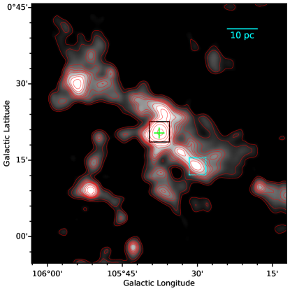
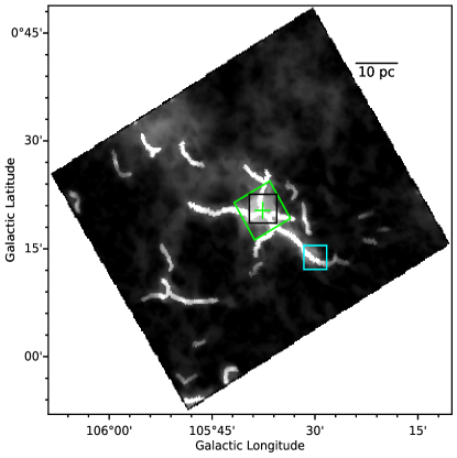
Figure 1: (left) CO(1-0) integrated intensity map in [-62.5,-41] km s^-1  velocity range. Contours have also been drawn (at 5, 7, 11, 12.5, 14, 15, 16.5, 20, 23, 27, 35, 45, and 65 K km s^-1) for clarity of the features. (right) Herschel 350 µm  image with overlaid skeletons of filaments identified by getsf. Black Box denotes the central portion where CO(1–0) spectrum has been extracted. Cyan box marks the CO clump which also (i.e. apart from the central region) corresponds to N(H₂) $\geq$ 10²² cm^-2 (see Figure 2). Green plus symbol shows the location of IRAS 22308+5812, and green box on the 350 µm  image shows the field of view of JCMT analysis (see Section 3.2).

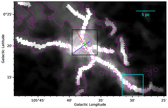
Figure 2: A zoomed in view of Figure 1. Magenta dashed and solid contours mark N(H₂) = 33$\times$10²⁰ cm^-2 and 10²² cm^-2, respectively, from the Vialactea maps. Dashed blue and red lines mark the major axes of blue and red outflow contours, respectively, from Qin et al. (2008). The rest of the symbols are same as Figure 1.

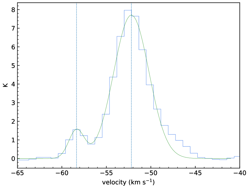
Figure 3: CO(1-0) spectrum at the central position marked in Figure 1. Green curve shows the gaussian fit, with dashed vertical lines marking the peak velocities of the two velocity components.

3 Analysis and Results

3.1 Large-scale view of the region

In this section, we explore the large-scale morphology as well as the hub-filament system in the region. Figure 1 shows the ¹²CO(1-0) moment-0 (integrated intensity) map of the larger region in the velocity range [-62.5,-41] km s^-1. The central core has been marked in a black box and the IRAS source (IRAS 22308+5812) with a green plus symbol. Multiple filamentary structures can be seen emanating from this central core, with each of them harbouring separate potential clumps of their own. To better understand the filamentary structure of the region, we used the getsf tool (version 211109) of Men’shchikov (2021). The tool, especially developed for Herschel images, decomposes an image into its structural components (sources and filaments) and separates them from their background. The method is fully automated and takes as input only one parameter from the user – the maximum size of the structure to extract. For our purpose, we used the Herschel 350 µm  image, and set the maximum size of filamentary structure to 550″  based on visual inspection. Figure 1 shows the Herschel 350 µm  image with the skeleton of filamentary structures identified by the getsf tool. It should be noted that the width associated with the skeletons on the image is only for visualisation purpose. It can be seen that the structures which appeared nearly contiguous in emission in the CO map (Figure 1), are detected as different (filamentary) structures in Figure 1. Figure 2 shows a zoomed in view of Figure 1 with overlaid column density contours from Vialactea map and the major axes of red and blue outflow lobes from Qin et al. (2008). According to the criteria of Myers (2009), the hub has low aspect ratio, and can be defined in terms of column density as the region where N(H₂) $\gtrsim$ 10²² cm^-2. As per this definition, the hub region here (solid magenta contour in Figure 2) occurs at the location where there is a joining of multiple filaments. Some of the getsf filaments are also traced by lower column density contour at 33$\times$10²⁰ cm^-2. However, the large scale view of the region shows that the filament sizes have an order of magnitude of $\sim$ 10 pc. This is in contrast with nearby HFS, where filaments have been found to have sizes of the order of magnitude of $\sim$ 1 pc (Arzoumanian, 2017; Arzoumanian et al., 2019). On the other hand, large filaments of sizes in tens of parsecs have also been recorded in literature (Zucker et al., 2018; Hacar et al., 2022). Nevertheless, as also discussed in Kumar et al. (2020), we would like to add the caveat that higher resolution studies of the region could resolve it into structures with similar hub/filament size scales as for the nearby regions.

Figure 3 shows the ¹²CO(1-0) line spectrum in the central region and the gaussian fit to its components. The first velocity component is at ($v\pm\sigma$) -58.4$\pm$0.9 km s^-1 with an amplitude of 1.5 K; while the second component is at -52.2$\pm$2.0 km s^-1 with an amplitude of 7.7 K. These two different velocity components have been observed in earlier studies as well (Wouterloot & Brand, 1989; Kerton & Brunt, 2003; Brunt et al., 2003). It must be noted that CO(1-0) emission is regarded as optically thick and often self-absorbed. Hence it is not used as a probe for the denser regions of the molecular cloud. For the central region, the stronger velocity component has a prominent broad wing towards the red side, which is probably an effect of the outflow.

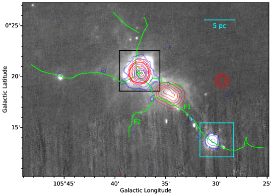
Figure 4: Herschel 70µm  image of the hub-filament system. Bolocam 1.1 mm emission is shown in blue dashed contours at 0.08, 0.1, 0.2, 0.4, 0.5, 0.7, 0.9, 1.0, and 1.4 Jy beam^-1. Red contours (at 0.002, 0.004, 0.007, 0.01, 0.013, 0.04, 0.08, 0.15, 0.3, and 0.4 Jy beam^-1) are for the NVSS 1.4 GHz emission. Green lines mark the getsf filamentary skeletons (see Figure 2). Green cross shows the location of the IRAS source, and “F1” and “F2” are the labels for the two respective filaments. The central black box and the cyan box are the same as in Figure 2.

Figure 4 shows the Herschel 70 µm  image of the region, overlaid with filament skeletons from the getsf tool (Figure 2), smoothed Bolocam 1.1 mm contours (in blue), and NVSS 1.4 GHz contours (in red). 70 µm  emission traces the warm dust emission due to stellar sources and is indicative of star formation in a region (Li et al., 2010; Calzetti, 2013). It can be seen that along the filament marked “F1” on the image, there appears to be star formation activity, as evidenced by the presence of bright diffused emission along its length. To the slight west of the point where the filament F1 joins filament F2, extended emission can be traced on the image, also seen in NVSS (red contours). The integrated flux density from the NVSS image was obtained to be 0.06 Jy, yielding a Lyman continuum flux of $\sim$ 10^47.2 photons s^-1 (Moran, 1983), which on comparison with the tabulated values from Panagia (1973) (assuming a Zero Age Main Sequence (ZAMS) single source) would suggest that a source of at least spectral type B0.5–B0 is required for the ionisation of the region. Though no massive stars have been found located in the immediate vicinity of this diffused ionised region, it is possible that there could be embedded massive star formation at the junction of filaments F1 and F2. The presence of a 1.1 mm clump at this junction could be an affirmation of this.

The filament F1 also hosts a few Bolocam 1.1 mm emission clumps along its length, especially at its south-west corner, where there appears to be a massive clump (within the cyan box). We retrieved the integrated flux density from the Bolocam Galactic Plane Survey Catalog v2.1 (Ginsburg et al., 2013) from the IRSA archive. Apart from the 1.1 mm emission in the central region (associated with IRAS 22308+5812), the catalog contains only the clump in the south-west in our field of view. Other contours depicting 1.1 mm emission might not have been included due to not meeting the catalog criteria (Ginsburg et al., 2013). Nevertheless, it is relevant to note their presence along the filaments. The retrieved integrated flux density was used to calculate the core total mass of gas and dust using the following formula (Hildebrand, 1983; Enoch et al., 2008; Bally et al., 2010) :

$$M=\frac{D^{2}~{}S_{\nu}~{}R_{t}}{B_{\nu}(T_{d})~{}\kappa_{\nu}},$$ (1)

where, D is the distance, S_ν is the integrated flux density, R${}_{\textup{t}}$ is the gas-to-dust mass ratio (taken as 100), B_ν(T${}_{\textup{d}}$) is the Planck function at dust temperature T${}_{\textup{d}}$ (taken as 10 K), and $\kappa_{\nu}$ is the dust opacity (1.14 cm² g^-1) (Enoch et al., 2006; Dewangan et al., 2016). The above equation assumes that the emission (at 1.1 mm here) is optically thin, and both T${}_{\textup{d}}$ and $\kappa_{\textup{1.1\,mm}}$ are position-independent within a core. Using the retrieved integrated flux densities of $\sim$ 8.316 Jy and 1.300 Jy for the central and south-western clumps, respectively, the resultant masses were calculated to be $\sim$ 10274 M_☉ and 1606 M_☉, respectively. The south-west Bolocam clump is also associated with a “hub”, as is evident in Figure 2 from the column density contour (solid magenta contour within the cyan box). We find that while the south-west Bolocam clump has mass of the order of magnitude similar to other hubs from literature (i.e. $\sim$10³ M_☉), such as Mon R2 (Treviño-Morales et al., 2019; Kumar et al., 2022), SDC13 (Williams et al., 2018), and others (Hacar et al., 2022), the mass for the central Bolocam clump is an order of magnitude larger. This is probably due to the fact that the integrated flux density covers a wider emission region (Rosolowsky et al., 2010) than the mere hub. If one were to use the flux density within 80″  diameter aperture for the central clump (area roughly coincident with N(H₂)$\sim$10²² cm^-2 hub region) – also given in the catalog ($\sim$3.814 Jy) – a mass of $\sim$ 4712 M_☉ is obtained, which is of the order of magnitude as for other studies in literature.

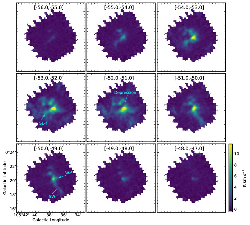
Figure 5: Channel maps of ¹³CO(3-2)  emission. Three filamentary structures – Western filament (W-f), South-West filament (SW-f), and South-East filament (SE-f) can be traced on the images. A region of minima in emission has been marked as “Depression” in the [-52,-51] km s^-1  channel map.

3.2 Molecular gas kinematics in the central region

We now examine the central part of the Sh2-138 region (see the field of view marked on Figure 1) using (spatial and spectral) higher resolution CO(3-2), ¹³CO(3-2), and C¹⁸O(3-2)  molecular line data retrieved from the JCMT archive. The field of view of each cube is $\sim$ 5′$\times$5′  and roughly encloses the hub and central core of CGPS CO emission. For ¹³CO and C¹⁸O, the rebinned cubes with 0.5 km s^-1  channel width have been used to examine the spatial structures in the following sections as their lower noise (see section 2) allows for better examination of features. However for the calculation of physical parameters (in section 3.2.4), the native channel width ($\sim$ 0.05 km s^-1) ¹³CO and C¹⁸O cubes have been utilised as we need high velocity resolution here.

Figure 5 shows the channel maps for the ¹³CO(3-2)  emission. The velocity range for each frame has been given. In the [-50,-49] km s^-1  velocity range, two prominent filamentary structures can be traced, and these have been indicated by arrows. The filament along the south-west direction (SW-f) is longer and much more prominent. It can only be seen in the -51 to -49 km s^-1  velocity range, and has no counterparts at larger or smaller velocities. The second filament, pointing west (W-f), is also seen prominently in -51 to -49 km s^-1 , but can be traced as diffused emission at larger and smaller velocities. As we move towards higher (absolute) velocities, a third filament can be traced in the -56 to -51 km s^-1  range in south-east direction (SE-f), and is most prominently seen in the [-53,-52] km s^-1  channel map. Apart from the filaments, another prominent feature is the sudden depression in emission - along the south-east to north-west axis - seen in the [-53,-52] and [-52,-51] km s^-1  channel maps. At larger and smaller velocity channel maps, this depression shows the presence of diffuse emission. It should be noted that the systemic velocity of the cloud complex is $\sim$ -51.7$\pm$1.9  km s^-1 (see Section 3.2.4). We note that the above-mentioned features (filaments and depression) could also be traced in the C¹⁸O(3-2)  channels, albeit not at the requisite signal-to-noise threshold (see section 3.2.1).

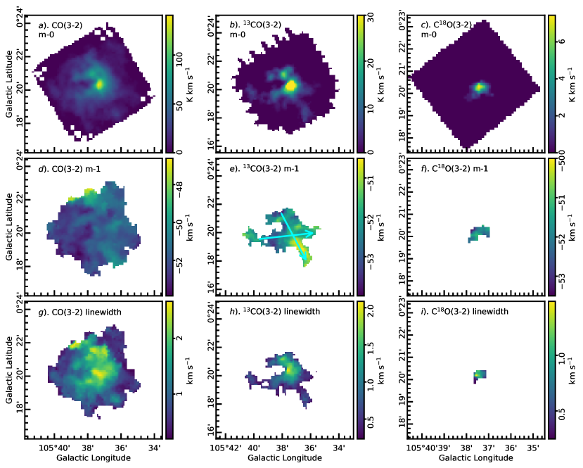
Figure 6: Row-wise : moment-0 (Integrated intensity), moment-1 (Intensity-weighted velocity), and linewidth (Intensity-weighted dispersion) collapsed images for three cubes – CO(3-2), ¹³CO(3-2), C¹⁸O(3-2)  in first, second, and third columns, respectively. Cyan vectors in ¹³CO(3-2)  moment-1 map mark the directions along which p-v slices have been extracted.

3.2.1 Moment maps

To account for the noise in the cubes, we confine our further analysis to only those regions with detections above 5$\sigma$ (where $\sigma$ is the data’s rms noise level). Using the clumpfind algorithm (Williams et al., 1994) as implemented in the cupid package (Berry et al., 2007) of starlink software suite (Currie et al., 2014), clumps were identified in the position-position-velocity spectral cube. The threshold for detection was kept conservatively at 5$\sigma$ to avoid the possibility of false detections, and the gap between contour levels at 2$\sigma$ as is recommended by Williams et al. (1994). The clumps detected in all three spectral cubes (CO(3-2), ¹³CO(3-2), and C¹⁸O(3-2)) lay in the range (-60,-45) km s^-1. Thereafter, the regions with non-detection were masked to construct masked cubes for all three molecular lines.

Figure 6 shows the moment-0 (Integrated emission), moment-1 (Intensity-weighted velocity), and linewidth (Intensity-weighted dispersion) collapsed images from all three (masked) cubes. In the intensity-weighted velocity map for CO(3-2), high-velocity gas is interspersed with low-velocity gas throughout and no particular pattern is discernible. For ¹³CO(3-2), as in the case of integrated intensity emission, filamentary structure is noticeable here as well. The filament along the south-west (SW-f, see Figure 5) shows a lower (absolute) velocity than other parts of the region. Such a velocity profile would suggest a gradient (at the joint between the SW-f filament and the central part) resulting in gas flow. To better understand the same, position-velocity slices were taken along the two vector directions (east-west and north-south) marked on this image, which we elaborate upon in section 3.2.2.

The intensity-weighted dispersion maps are shown in the last row of this image grid. The central part of the cloud shows a large velocity dispersion, of the order of about 2 km s^-1  in all three molecular lines, yet another indication of mixing of flows. This large dispersion is seen to extend along the north-east part of the image in both CO(3-2)  and ¹³CO(3-2)  molecular lines. In contrast, the south-west filament (traced prominently in ¹³CO(3-2) ) shows a relatively smaller dispersion of $\sim$1 km s^-1. CO(3-2)  is the most ubiquitous tracer of molecular hydrogen and shows diffused emission in the entire region in the integrated intensity map. ¹³CO(3-2)  has higher critical density and thus shows the filamentary nature prominently, while C¹⁸O(3-2)  which has the highest critical density primarily traces the central clump.

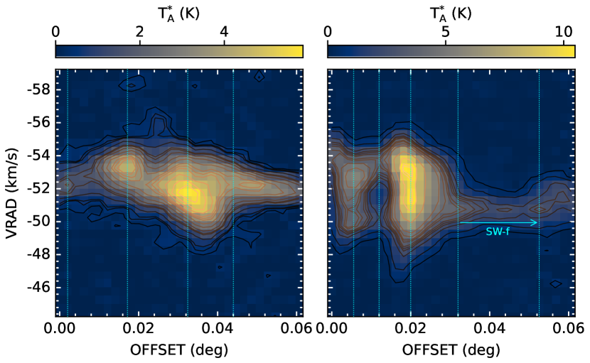
Figure 7: Position-velocity maps along the two vector directions marked in the ¹³CO(3-2)  intensity-weighted velocity map in Figure 6(e). Left : along the east-west vector (contours at 0.3, 0.5, 0.6, 1, 1.5, 1.65, 2, 2.5, 3, 3.5, 3.75, 4, 4.5, 5, 5.5, and 6 K). Right : along the north-south vector (contours at 0.45, 1, 2, 2.5, 2.75, 3, 3.5, 3.75, 4.25, 5, 7, 9, 10, and 10.25 K). Vertical dotted lines mark the intervals between which appreciable gradient can be seen. SW-f is the filament from Figure 5.

3.2.2 Position-velocity slices

Figure 7 shows the position-velocity (p-v) maps along the two directions marked in the ¹³CO(3-2)  intensity-weighted velocity map in Figure 6(e). The first figure shows the slice for the east-west vector and second for the north-south vector. Along both the slices, there appears to be a significant velocity gradient as one moves along the vector. Vertical dotted lines mark the intervals between which appreciable gradient can be seen. The east-west slice shows the absolute velocity increasing from $\sim$ 52 km s^-1  to 54 km s^-1, then decreasing to below 51 km s^-1  and then again increasing to above 52 km s^-1. A similar pattern is observed in the north-south slice, where the velocity first increases slightly and then decreases as one moves along the vector, i.e. from offset 0 degrees to 0.06 degrees ($\sim$ 6 pc). In Figure 7(left), the offset from $\sim$ 0.044 degree onwards is roughly coincident with the W-f filament, and in Figure 7(right), the offset from $\sim$ 0.032–0.052 degrees represents the SW-f filament (see ¹³CO(3-2)  moment-1 map in Figure 6(e)). As was also seen in the moment-1 map, the velocity is nearly constant at $\sim$ -52 km s^-1  and -51 km s^-1  along W-f and SW-f filaments, respectively. A small gradient is seen only towards the end for SW-f. This gradient coincides with the position of peak(s)/clump(s) (discussed below in section 3.2.3) and could thus denote gas being channeled into the clump. Overall, this gradient pattern in both the slices is indicative of gas spiralling into the central region from both the ends of the molecular cloud. There also appears to be clumping of gas, with the brightest clump (roughly at an offset of 0.032 degrees and 0.02 degrees in figures 7(left) and 7(right) respectively) being that of the central region. Another noticeable feature in the north-south slice (Figure 7(right)) is the presence of a dark region at an offset of $\sim$ 0.012 degrees in the velocity range -52 to -51 km s^-1. There is only a faint connecting feature between the immediate northern and southern clumps at $\sim$ -54 to -53 km s^-1. This dark region corresponds to the prominent gap seen in the channel map (marked “Depression” in the [-52, -51] km s^-1  channel map of Figure 5). In the central region, we find material clumping at two distinct velocities – -51 and -53 km s^-1. Overall, the maps show considerable dispersion in the velocity space around the systemic velocity of the cloud complex ($\sim$ -51.7 km s^-1 ), possibly due to the two directions being along the two outflow axes in the region (see section 4 for further discussion).

3.2.3 Analysis of ¹³CO(3-2)  and Herschel clumps

Figure 8 shows the ¹³CO(3-2)  integrated emission along with Herschel 250 µm  map of the region. Contours have been drawn on both the images for a better clarity of the features. Boxes on both the images mark the locations where spectra have been extracted. Since the beamsize is of the order of $\sim$2 pixels, spectra were extracted for a 2x2 box encompassing the pixel with the local maxima. Red boxes mark the regions which show a (local) peak in the ¹³CO(3-2)  integrated intensity map, while magenta boxes (c3, c4, c10, c13, c16) mark the locations of those peaks which are seen in 250 µm  but not traced clearly in the integrated intensity image. Blue boxes mark the locations which do not display any peak, but are along the filaments which can be delineated – c6 and c7 for the west-pointing filament (W-f in Figure 5), c8 and c9 for the south-west pointing filament (SW-f in Figure 5). The ¹³CO(3-2)  molecular line spectra extracted at these locations have been shown in Figure 9. For the central clump – marked c5 – C¹⁸O(3-2)  emission was also detected at above 5$\sigma$ threshold, and hence C¹⁸O(3-2)  molecular line spectrum has also been plotted for this location in Figure 9 (weaker step-line plot in the frame for c5). It should be noted that the massive stars studied by Deharveng et al. (1999); Baug et al. (2015) are associated with the location of c5.

An obvious feature to note here is that the locations c2, c4, and c5 show self-absorption near the peaks. While the spectrum for c5 (the central clump) is nearly symmetrical around the self-absorption “dip” in the spectrum, those for c2 and c4 are asymmetrical. The location c4 particularly seems to be having high self-absorption, indicative of dense material present in this part. It is worth noting that while the c4 clump is prominently observed in the thermal dust emission wavelength at 250 µm, the location shows a depression in ¹³CO(3-2)  molecular line emission. This can be seen in the integrated emission in Figure 8(left) as well as in the channel maps in Figure 5. c4 lies in the prominent gap marked in the [-52, -51] km s^-1  channel map of Figure 5. It is also almost coincident with the gap seen in the position-velocity slice (see Figure 7(right) at around an offset of 0.012 degrees) along the north-south vector (see intensity-weighted velocity map of ¹³CO(3-2)  in Figure 6(e)). We note that the weaker velocity component from the CGPS CO(1-0) spectra (see Figure 3) is barely seen and only for a few peaks (such as c8, c13, c14, c17, and c18) due to the weak nature of this emission. The low number of pixels used to extract spectra at these locations make this component virtually indistinguishable from the noise. An averaged spectrum over the entire JCMT field of view does indeed reveal this component (not shown here).

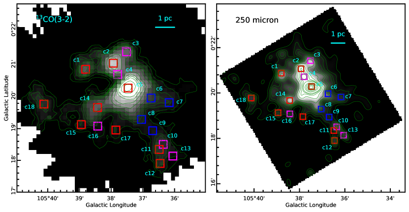
Figure 8: Left : ¹³CO(3-2)  integrated intensity map (contours at 0.45, 2, 4, 5, 6, 7, 10, 15, 20, 25, 30, 40, and 50 K km s^-1). Right : Herschel 250 µm  image (contours at 0.23, 0.3, 0.35, 0.4, 0.5, 0.6, 0.7, 1, 1.5, 2, 2.5, 3, 5, 7, 10, 12, and 15 $\times$10³ MJy sr^-1). Red boxes mark the peaks seen in the integrated intensity map while magenta boxes mark those which are primarily seen in the 250 µm  image (and are not noticeable in the first image). Blue boxes mark the locations which do not display any peak, but where spectra for W-f and SW-f (i.e. western and south-west filaments, Figure 5) were extracted.

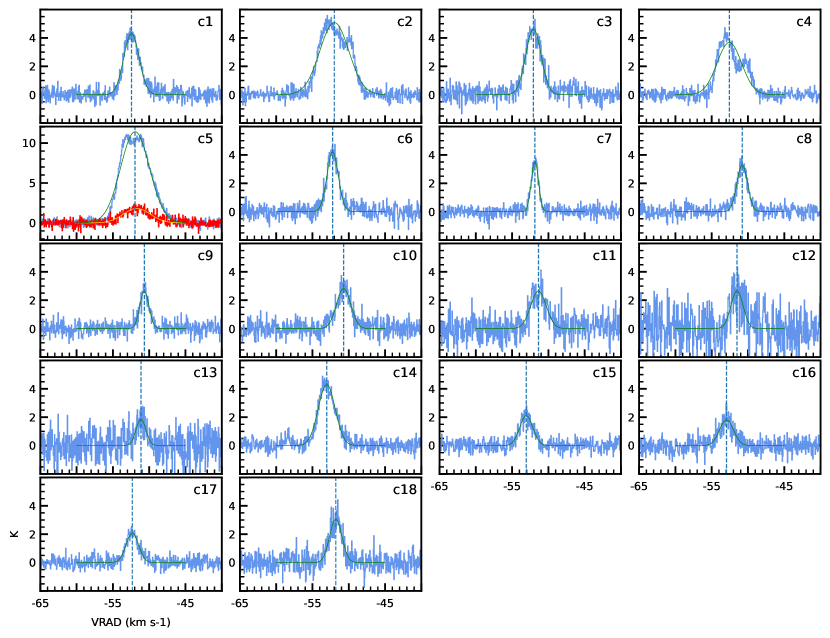
Figure 9: ¹³CO(3-2)  spectra at positions marked in Figure 8. Green curve depicts the gaussian fit to the spectra, with blue dashed line marking the velocity for the peak of the gaussian fit. For c5, C¹⁸O(3-2)  spectrum has been plotted in red and gaussian model fit shown with yellow curve.

3.2.4 Physical parameters

To extract the parameters for further calculations, we carried out gaussian model fitting for each region in the velocity range [-60,-45] km s^-1  on the (non-averaged) ¹³CO and C¹⁸O spectral cubes with native channel width of $\sim$ 0.05 km s^-1. The gaussian fits to the ¹³CO(3-2)  molecular line emission have been shown with a green line in all the spectra (Figure 9). The results of the model fitting of the clumps, along with other parameters, are listed in Table 2. As mentioned earlier, for the c5 central clump, C¹⁸O(3-2)  spectrum was also available, and has been shown as well along with its gaussian fit. Both the isotopologues were found to have similar peak velocities, $\sim$ -51.7$\pm$1.9 km s^-1  and -52$\pm$2 km s^-1  for C¹⁸O and ¹³CO, respectively. Since C¹⁸O traces the densest part of the cloud, its velocity can be taken as the systemic velocity of the cloud complex, and is in agreement with literature (Blitz et al., 1982; Burov et al., 1988; Harju et al., 1993; Bronfman et al., 1996; Johansson et al., 1994).

The gaussian model fit was used to obtain the FWHM (full width at half maxima) and standard deviation (or velocity dispersion) for each region. Thereafter, we calculate the non-thermal velocity dispersion and total velocity dispersion using the following equations (Fuller & Myers, 1992; Fiege & Pudritz, 2000) :

$$\Delta V_{tot}^{2} = \Delta V_{obs}^{2}+8~{}~{}ln\,2~{}~{}kT\left(\frac{1}{\bar{m}}-\frac{1}{m_{obs}}\right)$$ (2)

$$\Rightarrow\frac{\Delta V_{tot}^{2}}{8~{}~{}ln\,2} = \frac{kT}{\bar{m}}+\left(\frac{\Delta V_{obs}^{2}}{8~{}~{}ln\,2}-\frac{kT}{m_{obs}}\right)$$

$$\Rightarrow\sigma_{tot}^{2} = c_{s}^{2}+\left(\sigma_{obs}^{2}-\sigma_{\textsc{t}}^{2}\right)$$ (3)

$$= c_{s}^{2}+\sigma_{\textsc{nt}}^{2}$$ (4)

where, $\Delta V_{obs}$ and $\sigma_{obs}$ ($=\Delta V_{obs}/\sqrt{8ln\,2}~{}$ for a gaussian) are the FWHM and standard deviation (or dispersion), respectively, from the observed spectrum of the molecular species; $\sigma_{\textsc{t}}(=\sqrt{kT/m_{obs}})$ is the thermal velocity dispersion for the molecular species; $m_{obs}$ is the mass of the molecule (29 amu and 30 amu for ¹³CO and C¹⁸O respectively); $\sigma_{\textsc{nt}}$ is the non-thermal velocity dispersion; $c_{s}$($=\sqrt{kT/\bar{m}}$) is the speed of sound; $\bar{m}$ is the average molecular weight of the medium (2.37 amu); and T is the excitation or gas kinetic temperature.

The critical density for ¹³CO(3-2)  is in the range $\sim$ 10^4-5 cm^-3, and if we assume the gas and dust temperatures to be coupled via collisions at this density (Goldsmith, 2001), then the dust temperature from Herschel Vialactea temperature map can be used for gas kinetic temperature T in the above equation. We add a caveat though that, depending on the physical conditions of the region, a significant difference between the gas and dust temperatures can still exist (Banerjee et al., 2006; Koumpia et al., 2015). The median temperature at the locations of the peaks ranged from 18-20 K (c_s $\sim$0.25–0.27 km s^-1), with the c4 and c5 clumps at 28 K (c_s $\sim$0.31 km s^-1). At these temperatures, the thermal velocity dispersion $\sigma_{\textsc{t}}$ (for both ¹³CO and C¹⁸O) comes out to be $\sim$0.07–0.09 km s^-1. Table 2 lists these calculated values for the clumps associated with the peaks in Figure 8.

The FWHM values for almost all the peaks lie in the $\sim$ 2-2.75 km s^-1  range (and thus $\sigma_{obs}\sim$0.85-1.2 km s^-1), except for c2, c4, and c5 which lie in $\sim$4-4.7 km s^-1($\sigma_{obs}\sim$1.7-2 km s^-1). This was also observed in the linewidth map in Figure 6(h). For c13, the lower value might be due to the noisy spectrum. As $\sigma_{obs}$ is much larger than $\sigma_{\textsc{t}}$ (0.07–0.09 km s^-1) for all the cases, we find it to be almost same as $\sigma_{\textsc{nt}}$. c2, c4, and c5 locations have the highest non-thermal dispersions. Using the above variables, we subsequently calculated the Mach number ($=\sigma_{\textsc{nt}}/c_{s}$) and the ratio of thermal to non-thermal pressure ($P_{\textsc{tnt}}=c_{s}^{2}/\sigma_{\textsc{nt}}^{2}$) as well (Lada et al., 2003). All the locations were found to have Mach numbers which suggest supersonic motion, with c2 and c5 displaying the largest values ($\gtrsim$6). The order of magnitude of P${}_{\textsc{tnt}}$ ($\sim$0.01–0.1) indicates that non-thermal pressure dominates in the cloud, and the locations of highest non-thermal dispersion and Mach numbers (i.e. c2, c4, and c5) were found to be correlated to the least ratio values.

Myers (2009) posit a hub-filament model of star-forming complexes where the hub (Kumar et al., 2020) is traced at a high column density of $\sim$ 10²² cm^-2 as opposed to the filaments (André, 2013; Arzoumanian et al., 2013) which have a column density of $\sim$ 10²¹ cm^-2. For the three filaments – SW-f, W-f, and SE-f (see Figure 5) – we calculated the line mass using the Herschel column density map constructed from thermal dust emission (see Section 2). The length of the three filaments was taken from the 10²² cm^-2 contour (i.e. the inner extent) along the line joining c6 and c7 for W-f; c8, c9, and c10 for SW-f; and upto c14 for SE-f. Total column density was summed up in a width of 12″  (corresponding to $\sim$ 0.33 pc at a distance of 5.7 kpc) as it is the resolution of the column density map. Thereafter, using the following formula (Mallick et al., 2015; Dewangan et al., 2017b) :

$$M_{line,obs}=\frac{\mu_{\textsc{h${}_{2}$}}~{}m_{\textsc{h}}~{}Area_{pixel}~{}\Sigma N(H_{2})}{\textup{(length of filament)}}$$ (5)

– where $\mu_{\textsc{h${}_{2}$}}$ is the mean molecular weight (2.8), m${}_{\textsc{h}}$ is the mass of Hydrogen, Area_pixel is the area subtended by one pixel, and $\Sigma N(H_{2})$ is the total column density – we calculated the (observed) line masses to be $\sim$ 32, 33.5, and 50 M_☉ pc^-1 for the filaments W-f, SW-f, and SE-f, respectively.

Table 2: Parameters derived from ¹³CO(3-2)  spectra at the locations of peaks in Figure 8. For c5, C¹⁸O(3-2)  spectrum was also available and thus used for calculation as well.

clump	FWHM	T	$\sigma_{\textsc{nt}}$	Mach	$P_{\textsc{tnt}}$
	($km~{}s^{-1}$)	(K)	($km~{}s^{-1}$)	Number
c1	2.48	20	1.05	3.97	0.06
c2	4.71	20	2.00	7.55	0.02
c3	2.50	20	1.06	3.99	0.06
c4	3.98	28	1.69	5.39	0.03
c5
C18O	4.39	28	1.86	5.95	0.03
13CO	4.69	28	1.99	6.35	0.03
c10	2.30	18	0.98	3.88	0.07
c11	2.53	18	1.07	4.26	0.05
c12	1.97	18	0.83	3.31	0.09
c13	1.60	18	0.68	2.69	0.14
c14	2.75	20	1.17	4.40	0.05
c15	2.14	18	0.91	3.61	0.08
c16	2.27	18	0.96	3.83	0.07
c17	2.03	18	0.86	3.42	0.09
c18	1.99	18	0.84	3.35	0.09

4 Discussion

According to the multiwavelength study of Baug et al. (2015), Sh2-138 represents the archetype “hub-filament” structure of Myers (2009) which – after the advent of Herschel far-infrared data – has been found to be a ubiquitous feature of young stellar clusters hosting low-mass and high-mass stars (Kumar et al., 2020). However, this interpretation needs to be tempered by the fact that most of the filamentary clouds whose intricate structure has been studied in literature have been nearby regions such as Monoceros R2 (Treviño-Morales et al., 2019, 830 pc), W40 (Mallick et al., 2013, 500 pc), IC 5146 (Arzoumanian et al., 2011, 460 pc), and others (Arzoumanian et al., 2019; Hacar et al., 2022). Though regions at further distances have been explored in literature, such as IRAS 05480+2545 (Dewangan et al., 2017a, 2.1 kpc), Sh2-53 (Baug et al., 2018, 4 kpc), G18.88–0.49 (Dewangan et al., 2020, 5 kpc) and so on, the larger distance often makes it difficult to resolve finer structures. The large scale view of the Sh2-138 region shows filaments whose sizes are of the order of $\sim$ 10 pc. Such large filaments (at distances of a few kpc) have also been discussed in various studies – with Nessie cloud often held up as an archetype; and terminologies such as “Giant Molecular Filaments” and “Milky Way Bone” have been employed for such large filaments (Ragan et al., 2014; Zucker et al., 2018). Nevertheless, as also discussed in Kumar et al. (2020), it is possible that higher resolution studies of distant regions could resolve a large filament into structures with size scales as for the nearby regions. The higher resolution JCMT and Herschel maps for the central region seem to suggest this where we can see more detailed structures. The filamentary structures in the central region have sizes of the order of a few parsecs, which is not so uncommon. Examples of some of the massive star forming regions from literature where such length scales have been observed are G22 (Yuan et al., 2018, 3.51 kpc), DR21 (Hennemann et al., 2012, 1.4 kpc), SDC13 (Peretto et al., 2014, 3.6 kpc), though the line masses for these regions are larger with a wide range, varying from $\sim$ 2 upto 20 times our line masses. On the other hand, nearby regions such as IC 5146 (Arzoumanian et al., 2011, 460 pc) show a wide span of line masses for filaments of lengths of a few parsecs, from $\sim$ 0.5 to 3 times our line masses.

Hacar et al. (2022) have used a census of more than 22000 filaments from literature to categorise them into different (non-mutually exclusive) families. A comparison of the structure and physical parameters of the filamentary structures in Sh2-138 with their compilation shows that while our filaments are similar to “Dense Fiber” filament family in their categorisation in terms of being structures in position-position-velocity space, our filaments display a larger non-thermal dispersion ($\sigma_{\textsc{nt}}$). Higher $\sigma_{\textsc{nt}}$ values are seen for “Galactic plane survey filaments” and “Giant filaments” (see Table 2 of Hacar et al., 2022). As discussed for these two filament families in Hacar et al. (2022), the calculation of physical parameters could suffer from sensitivity and resolution biases, given the 5.7 kpc distance for the region, as well as be affected by the tracer used for calculations. High values of $\sigma_{\textsc{nt}}$ and Mach number have been determined to be a result of large-scale accretion flows resulting in internal turbulence, and when filament networks (with disparate velocity centroids) are observed with low-resolution beams, the resulting measurements of linewidth are expected to be supersonic (Hacar et al., 2016).

The central part of the Sh2-138 region has been mapped by JCMT CO(3-2), ¹³CO(3-2), and C¹⁸O(3-2)  molecular lines. These molecular lines trace the warm and dense gas – in the temperature range 10-50 K and density $\sim$ 10^4-5 cm^-3 – enveloping the cores where star formation is taking place (Davis et al., 2010). Three main filaments – labelled W-f, SW-f, and SE-f – can be traced on the ¹³CO(3-2)  channel map (Figure 5). While one end of SW-f and SE-f filaments merges into the hub, the morphology at other end of these two filamentary structures shows other possible filaments branching from them. For example, in Figure 8, SW-f (“c8-c9-c10”) filament seems to be branching into “c10-c11-c12” and “c10-c13”; and SE-f seems to be branching into “c14-c15” and “c14-c16”. It is possible that they represent secondary filaments which merge into primary filament (SW-f and SE-f here), which then merges into the hub. Such structure has been seen for regions like Monoceros R2 (Treviño-Morales et al., 2019; Kumar et al., 2022). Furthermore, at the end of SW-f in Figure 7(right), a clump is seen at an offset of $\sim$ 0.052 degrees (marked with a dashed vertical line). This clump corresponds to $\sim$ c10/c11 in Figure 8, which seems to be accreting matter from further along the filament length, given the small gradient which is seen in the 0.052-0.06 degree offset range in Figure 7(right). Along the length of the W-f and SW-f filaments marked in the p-v diagrams Figures 7(left) and 7(right), respectively, clumping of gas can also be seen. The p-v maps (Figure 7) show a velocity gradient as one approaches the central clump region, which indicates gas being channeled from outer regions to the central region. The relatively large velocity dispersion in the central part of the cloud in all three isotopologues (Figure 6) is indicative of this. The scenario that emerges is that of longitudinal flow along filaments converging on a stellar cluster (Peretto et al., 2014; Treviño-Morales et al., 2019; Kumar et al., 2020).

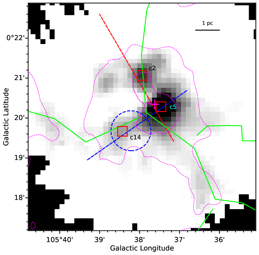
Figure 10: JCMT ¹³CO(3-2)  integrated intensity map. Magenta dashed and solid contours mark N(H₂) = 33$\times$10²⁰ cm^-2 and 10²² cm^-2, respectively, from the Vialactea maps. Dashed blue and red lines mark the major axes of blue and red outflow contours, respectively, from Qin et al. (2008). Magenta plus symbol shows the location of IRAS 22308+5812. Green lines are filament skeletons from Figure 2. The clumps c2, c5, and c14 from Figure 8 have been marked in by red boxes and labelled.

Figure 10 shows the JCMT ¹³CO(3-2)  integrated intensity map with overlaid column density contours, outflow axes, and the getsf filamentary skeletons from Figure 2 within this field of view. The peak of the blueshifted outflow emission has been indicated by a dashed blue circle and it coincides with the peak c14 from Figure 8. The trapezium-like cluster from Deharveng et al. (1999) (including a Herbig Be star; Baug et al., 2015), is coincident with the IRAS source marked here, which being far away from the blue lobe peak is unlikely to be the driving source of the blue outflow lobe. The cluster of young stellar objects (in which some are of intermediate mass) identified by Baug et al. (2015) which lie within the area of the blue lobe peak could be partially driving the outflow, or alternatively, c14 could be a source in the initial stages of star formation. As such, this source could be a suitable candidate as a subject of detailed investigation. Comparing Figures 6 and 10, one can see that the northern (eastern) part of the N-S (E-W) vector in Figure 6(e) is almost coincident with the red (blue) lobe axis in Figure 10. Thus the complex structure in the p-v diagram seen in Figure 7(right) ($\sim$ offset 0.00 to 0.02 deg, corresponding to northern part of the N-S vector of Figure 6(e)) could be a combination of the turbulence injected along the directions by the outflow and/or phenomena such as Hubble flow (Ridge & Moore, 2001; Arce & Goodman, 2001), mass entrainment, and so on (Lada & Fich, 1996; Arce & Goodman, 2002). Zinchenko et al. (2020) in their study of S255IR high-mass star forming region have observed that walls around outflow cavities could appear as filaments in projection. Given the arrangement of getsf filaments and outflow axes for the Sh2-138 region (in Figure 10), such a situation is also a possibility here and merits further investigation of the region in different molecular species. It is also worth noting that the central hub region (magenta solid contour in Figure 10) seems to have two centers (c2 and c5), also seen in other regions such as NGC 2264 (Kumar et al., 2020) and G31.41+0.31 (Beltrán et al., 2022).

Looking at the combined large-scale field-of-view (Section 3.1) and the central portion (Section 3.2) from the context of star-formation frameworks, one finds that there could be applicability of scenarios such as the Global Hierarchical Collapse (GHC Vázquez-Semadeni et al., 2019), the “Conveyor Belt” model (Longmore et al., 2014; Krumholz & McKee, 2020), and the HFS model (Kumar et al., 2020) based on the longitudinal flows. There also appears to be isolated star-formation all along the filament F1 in Figure 4, and though the isolated 1.1 mm emission clump seems to be associated with a hub (based on the column density), it does not come across as lying at any junction of filaments. A caveat, however, could be that merging filaments at this clump are directed nearly orthogonal to the plane of the sky in the line of sight. Finally, we note that there are studies in literature which – based on molecular line spectra – have suggested the existence of multiple clouds in various regions and subsequent “cloud-cloud-collision”, wherein collision between molecular clouds leads to a shock-compressed layer with density enhancement, due to which filament formation as well as high-mass star formation can occur (Scoville et al., 1986; Habe & Ohta, 1992; Tan, 2000; Anathpindika, 2010; Inoue & Fukui, 2013; Takahira et al., 2014; Fukui et al., 2021). Though multiple peaks in the CO spectra are seen for this region too (Section 3.1), such a scenario however, is tough to conclude, and would need observations in molecules which trace the dense gas of shock-compressed layers, such as NH₃ and HCN (Priestley & Whitworth, 2021) to justify.

5 Summary and Conclusions

In this paper we have carried out a molecular line study of the “hub-filament” system in the Sh2-138 region. The primary data utilised was CO(1-0) transition from CGPS for the wider $\sim$ 50′$\times$50′  region, and CO(3-2), ¹³CO(3-2), and C¹⁸O(3-2)  transitions from the JCMT archive for the central $\sim$ 5′$\times$5′  region. The main conclusions are as follows :

1. CGPS CO(1-0) integrated intensity emission of the region shows it to be a HFS of $\sim$ a few 10s of pc in scale. The central region shows a spectrum with two velocity components. The axes of outflows in the region from literature were found to be aligned along the filaments detected via the getsf tool.

2. In the large-scale field-of-view, one of the filaments (labelled “F1” in our analysis) appears to be a site of active star formation. It is associated with diffused ionised emission at a junction with another filament (labelled “F2”) and was found to be hosting a 1.1 mm emission clump of mass $\sim$ 1606 M_☉.

3. Analysis of the central $\sim$ 5′$\times$5′  area in ¹³CO(3-2)  emission found three filamentary structures – labelled W-f, SW-f, and SE-f – above a 5$\sigma$ detection threshold. The observed line mass (M${}_{\textup{line,obs}}$) was calculated to be $\sim$ 50, 32, and 33.5 M_☉ pc^-1 for SE-f, W-f, and SW-f, respectively.

4. The clump labelled c14, detected in Herschel 250 µm  emission as well as ¹³CO(3-2)  integrated intensity emission (at $>$ 5$\sigma$) was found to coincide with the peak emission region of the blue outflow lobe, and merits future investigation as a protostellar candidate.

5. Position-velocity slices (east-west and north-south slice) across the filaments revealed velocity gradients which point towards longitudinal flow along the filaments converging onto the central dense clump.

6. A gaussian model fitting of the spectra at different locations showed a dominance of non-thermal motion – with a large non-thermal dispersion and a small value of the ratio of thermal to non-thermal pressure ($\sim$ 0.01–0.1). Mach number ($\gtrsim$3) analysis indicates the presence of large supersonic motions within the clumps.

References

- Aguirre et al. (2011) Aguirre, J. E., Ginsburg, A. G., Dunham, M. K., et al. 2011, ApJS, 192, 4, doi: 10.1088/0067-0049/192/1/4
- Anathpindika (2010) Anathpindika, S. V. 2010, MNRAS, 405, 1431, doi: 10.1111/j.1365-2966.2010.16541.x
- Anderson et al. (2014) Anderson, L. D., Bania, T. M., Balser, D. S., et al. 2014, ApJS, 212, 1, doi: 10.1088/0067-0049/212/1/1
- André (2013) André, P. 2013, ArXiv e-prints. https://arxiv.org/abs/1309.7762
- Arce & Goodman (2001) Arce, H. G., & Goodman, A. A. 2001, ApJ, 554, 132, doi: 10.1086/321334
- Arce & Goodman (2002) —. 2002, ApJ, 575, 911, doi: 10.1086/341427
- Arzoumanian (2017) Arzoumanian, D. 2017, arXiv e-prints, arXiv:1712.00604. https://arxiv.org/abs/1712.00604
- Arzoumanian et al. (2013) Arzoumanian, D., André, P., Peretto, N., & Könyves, V. 2013, A&A, 553, A119, doi: 10.1051/0004-6361/201220822
- Arzoumanian et al. (2011) Arzoumanian, D., André, P., Didelon, P., et al. 2011, A&A, 529, L6, doi: 10.1051/0004-6361/201116596
- Arzoumanian et al. (2019) Arzoumanian, D., André, P., Könyves, V., et al. 2019, A&A, 621, A42, doi: 10.1051/0004-6361/201832725
- Bally et al. (2010) Bally, J., Aguirre, J., Battersby, C., et al. 2010, ApJ, 721, 137, doi: 10.1088/0004-637X/721/1/137
- Banerjee et al. (2006) Banerjee, R., Pudritz, R. E., & Anderson, D. W. 2006, MNRAS, 373, 1091, doi: 10.1111/j.1365-2966.2006.11089.x
- Baug et al. (2015) Baug, T., Ojha, D. K., Dewangan, L. K., et al. 2015, MNRAS, 454, 4335, doi: 10.1093/mnras/stv2269
- Baug et al. (2018) Baug, T., Dewangan, L. K., Ojha, D. K., et al. 2018, ApJ, 852, 119, doi: 10.3847/1538-4357/aaa429
- Beltrán et al. (2022) Beltrán, M. T., Rivilla, V. M., Kumar, M. S. N., Cesaroni, R., & Galli, D. 2022, A&A, 660, L4, doi: 10.1051/0004-6361/202243361
- Berry et al. (2007) Berry, D. S., Reinhold, K., Jenness, T., & Economou, F. 2007, in Astronomical Society of the Pacific Conference Series, Vol. 376, Astronomical Data Analysis Software and Systems XVI, ed. R. A. Shaw, F. Hill, & D. J. Bell, 425
- Beuther et al. (2007) Beuther, H., Churchwell, E. B., McKee, C. F., & Tan, J. C. 2007, in Protostars and Planets V, ed. B. Reipurth, D. Jewitt, & K. Keil, 165. https://arxiv.org/abs/astro-ph/0602012
- Blitz et al. (1982) Blitz, L., Fich, M., & Stark, A. A. 1982, ApJS, 49, 183, doi: 10.1086/190795
- Bolatto et al. (2013) Bolatto, A. D., Wolfire, M., & Leroy, A. K. 2013, ARA&A, 51, 207, doi: 10.1146/annurev-astro-082812-140944
- Bronfman et al. (1996) Bronfman, L., Nyman, L. A., & May, J. 1996, A&AS, 115, 81
- Brunt et al. (2003) Brunt, C. M., Kerton, C. R., & Pomerleau, C. 2003, ApJS, 144, 47, doi: 10.1086/344245
- Buckle et al. (2009) Buckle, J. V., Hills, R. E., Smith, H., et al. 2009, MNRAS, 399, 1026, doi: 10.1111/j.1365-2966.2009.15347.x
- Buckle et al. (2010) Buckle, J. V., Curtis, E. I., Roberts, J. F., et al. 2010, MNRAS, 401, 204, doi: 10.1111/j.1365-2966.2009.15619.x
- Burov et al. (1988) Burov, A. B., Kislyakov, A. G., Krasilnikov, A. A., et al. 1988, Soviet Astronomy Letters, 14, 209
- Calzetti (2013) Calzetti, D. 2013, in Secular Evolution of Galaxies, ed. J. Falcón-Barroso & J. H. Knapen, 419
- Cesaroni et al. (1988) Cesaroni, R., Palagi, F., Felli, M., et al. 1988, A&AS, 76, 445
- Condon et al. (1998) Condon, J. J., Cotton, W. D., Greisen, E. W., et al. 1998, AJ, 115, 1693, doi: 10.1086/300337
- Currie et al. (2014) Currie, M. J., Berry, D. S., Jenness, T., et al. 2014, in Astronomical Society of the Pacific Conference Series, Vol. 485, Astronomical Data Analysis Software and Systems XXIII, ed. N. Manset & P. Forshay, 391
- Davis et al. (2010) Davis, C. J., Chrysostomou, A., Hatchell, J., et al. 2010, MNRAS, 405, 759, doi: 10.1111/j.1365-2966.2010.16499.x
- Deharveng et al. (1999) Deharveng, L., Zavagno, A., Nadeau, D., Caplan, J., & Petit, M. 1999, A&A, 344, 943
- Dewangan et al. (2017a) Dewangan, L. K., Ojha, D. K., & Baug, T. 2017a, ApJ, 844, 15, doi: 10.3847/1538-4357/aa79a5
- Dewangan et al. (2016) Dewangan, L. K., Ojha, D. K., Luna, A., et al. 2016, ApJ, 819, 66, doi: 10.3847/0004-637X/819/1/66
- Dewangan et al. (2020) Dewangan, L. K., Ojha, D. K., Sharma, S., et al. 2020, ApJ, 903, 13, doi: 10.3847/1538-4357/abb827
- Dewangan et al. (2017b) Dewangan, L. K., Ojha, D. K., Zinchenko, I., Janardhan, P., & Luna, A. 2017b, ApJ, 834, 22, doi: 10.3847/1538-4357/834/1/22
- Dickinson et al. (1974) Dickinson, D. F., Frogel, J. A., & Persson, S. E. 1974, ApJ, 192, 347, doi: 10.1086/153065
- Enoch et al. (2008) Enoch, M. L., Evans, Neal J., I., Sargent, A. I., et al. 2008, ApJ, 684, 1240, doi: 10.1086/589963
- Enoch et al. (2006) Enoch, M. L., Young, K. E., Glenn, J., et al. 2006, ApJ, 638, 293, doi: 10.1086/498678
- Fich (1993) Fich, M. 1993, ApJS, 86, 475, doi: 10.1086/191787
- Fiege & Pudritz (2000) Fiege, J. D., & Pudritz, R. E. 2000, MNRAS, 311, 85, doi: 10.1046/j.1365-8711.2000.03066.x
- Fish (2007) Fish, V. L. 2007, in Astrophysical Masers and their Environments, ed. J. M. Chapman & W. A. Baan, Vol. 242, 71–80, doi: 10.1017/S1743921307012604
- Fukui et al. (2021) Fukui, Y., Habe, A., Inoue, T., Enokiya, R., & Tachihara, K. 2021, PASJ, 73, S1, doi: 10.1093/pasj/psaa103
- Fuller & Myers (1992) Fuller, G. A., & Myers, P. C. 1992, ApJ, 384, 523, doi: 10.1086/170894
- Ginsburg et al. (2013) Ginsburg, A., Glenn, J., Rosolowsky, E., et al. 2013, ApJS, 208, 14, doi: 10.1088/0067-0049/208/2/14
- Goldsmith (2001) Goldsmith, P. F. 2001, ApJ, 557, 736, doi: 10.1086/322255
- Graves et al. (2010) Graves, S. F., Richer, J. S., Buckle, J. V., et al. 2010, MNRAS, 409, 1412, doi: 10.1111/j.1365-2966.2010.17140.x
- Griffin et al. (2010) Griffin, M. J., Abergel, A., Abreu, A., et al. 2010, A&A, 518, L3, doi: 10.1051/0004-6361/201014519
- Habe & Ohta (1992) Habe, A., & Ohta, K. 1992, PASJ, 44, 203
- Hacar et al. (2016) Hacar, A., Alves, J., Burkert, A., & Goldsmith, P. 2016, A&A, 591, A104, doi: 10.1051/0004-6361/201527319
- Hacar et al. (2022) Hacar, A., Clark, S., Heitsch, F., et al. 2022, arXiv e-prints, arXiv:2203.09562. https://arxiv.org/abs/2203.09562
- Harju et al. (1993) Harju, J., Walmsley, C. M., & Wouterloot, J. G. A. 1993, A&AS, 98, 51
- Hennemann et al. (2012) Hennemann, M., Motte, F., Schneider, N., et al. 2012, A&A, 543, L3, doi: 10.1051/0004-6361/201219429
- Heyer et al. (1998) Heyer, M. H., Brunt, C., Snell, R. L., et al. 1998, ApJS, 115, 241, doi: 10.1086/313086
- Hildebrand (1983) Hildebrand, R. H. 1983, QJRAS, 24, 267
- Inoue & Fukui (2013) Inoue, T., & Fukui, Y. 2013, ApJ, 774, L31, doi: 10.1088/2041-8205/774/2/L31
- Inutsuka & Miyama (1997) Inutsuka, S.-i., & Miyama, S. M. 1997, ApJ, 480, 681, doi: 10.1086/303982
- Johansson et al. (1994) Johansson, L. E. B., Olofsson, H., Hjalmarson, A., Gredel, R., & Black, J. H. 1994, A&A, 291, 89
- Kerton & Brunt (2003) Kerton, C. R., & Brunt, C. M. 2003, A&A, 399, 1083, doi: 10.1051/0004-6361:20021826
- Koumpia et al. (2015) Koumpia, E., Harvey, P. M., Ossenkopf, V., et al. 2015, A&A, 580, A68, doi: 10.1051/0004-6361/201525669
- Krumholz & McKee (2020) Krumholz, M. R., & McKee, C. F. 2020, MNRAS, 494, 624, doi: 10.1093/mnras/staa659
- Kumar et al. (2022) Kumar, M. S. N., Arzoumanian, D., Men’shchikov, A., et al. 2022, A&A, 658, A114, doi: 10.1051/0004-6361/202140363
- Kumar et al. (2006) Kumar, M. S. N., Keto, E., & Clerkin, E. 2006, A&A, 449, 1033, doi: 10.1051/0004-6361:20053104
- Kumar et al. (2020) Kumar, M. S. N., Palmeirim, P., Arzoumanian, D., & Inutsuka, S. I. 2020, A&A, 642, A87, doi: 10.1051/0004-6361/202038232
- Kurtz (2002) Kurtz, S. 2002, in Astronomical Society of the Pacific Conference Series, Vol. 267, Hot Star Workshop III: The Earliest Phases of Massive Star Birth, ed. P. Crowther, 81. https://arxiv.org/abs/astro-ph/0111351
- Lada et al. (2003) Lada, C. J., Bergin, E. A., Alves, J. F., & Huard, T. L. 2003, ApJ, 586, 286, doi: 10.1086/367610
- Lada & Fich (1996) Lada, C. J., & Fich, M. 1996, ApJ, 459, 638, doi: 10.1086/176929
- Li et al. (2010) Li, Y., Calzetti, D., Kennicutt, R. C., et al. 2010, ApJ, 725, 677, doi: 10.1088/0004-637X/725/1/677
- Longmore et al. (2014) Longmore, S. N., Kruijssen, J. M. D., Bastian, N., et al. 2014, in Protostars and Planets VI, ed. H. Beuther, R. S. Klessen, C. P. Dullemond, & T. Henning, 291, doi: 10.2458/azu_uapress_9780816531240-ch013
- Mallick et al. (2013) Mallick, K. K., Kumar, M. S. N., Ojha, D. K., et al. 2013, ApJ, 779, 113, doi: 10.1088/0004-637X/779/2/113
- Mallick et al. (2015) Mallick, K. K., Ojha, D. K., Tamura, M., et al. 2015, MNRAS, 447, 2307, doi: 10.1093/mnras/stu2584
- Marsh et al. (2015) Marsh, K. A., Whitworth, A. P., & Lomax, O. 2015, MNRAS, 454, 4282, doi: 10.1093/mnras/stv2248
- Marsh et al. (2017) Marsh, K. A., Whitworth, A. P., Lomax, O., et al. 2017, MNRAS, 471, 2730, doi: 10.1093/mnras/stx1723
- Martín-Hernández et al. (2002) Martín-Hernández, N. L., Peeters, E., Morisset, C., et al. 2002, A&A, 381, 606, doi: 10.1051/0004-6361:20011504
- Men’shchikov (2021) Men’shchikov, A. 2021, A&A, 649, A89, doi: 10.1051/0004-6361/202039913
- Molinari et al. (2010) Molinari, S., Swinyard, B., Bally, J., et al. 2010, PASP, 122, 314, doi: 10.1086/651314
- Moran (1983) Moran, J. M. 1983, Rev. Mexicana Astron. Astrofis., 7, 95
- Motte et al. (2018) Motte, F., Bontemps, S., & Louvet, F. 2018, ARA&A, 56, 41, doi: 10.1146/annurev-astro-091916-055235
- Myers (2009) Myers, P. C. 2009, ApJ, 700, 1609, doi: 10.1088/0004-637X/700/2/1609
- Palagi et al. (1993) Palagi, F., Cesaroni, R., Comoretto, G., Felli, M., & Natale, V. 1993, A&AS, 101, 153
- Panagia (1973) Panagia, N. 1973, AJ, 78, 929, doi: 10.1086/111498
- Peretto et al. (2014) Peretto, N., Fuller, G. A., André, P., et al. 2014, A&A, 561, A83, doi: 10.1051/0004-6361/201322172
- Poglitsch et al. (2010) Poglitsch, A., Waelkens, C., Geis, N., et al. 2010, A&A, 518, L2, doi: 10.1051/0004-6361/201014535
- Portegies Zwart et al. (2010) Portegies Zwart, S. F., McMillan, S. L. W., & Gieles, M. 2010, ARA&A, 48, 431, doi: 10.1146/annurev-astro-081309-130834
- Priestley & Whitworth (2021) Priestley, F. D., & Whitworth, A. P. 2021, MNRAS, 506, 775, doi: 10.1093/mnras/stab1777
- Qin et al. (2008) Qin, S.-L., Wang, J.-J., Zhao, G., Miller, M., & Zhao, J.-H. 2008, A&A, 484, 361, doi: 10.1051/0004-6361:20078483
- Ragan et al. (2014) Ragan, S. E., Henning, T., Tackenberg, J., et al. 2014, A&A, 568, A73, doi: 10.1051/0004-6361/201423401
- Ridge & Moore (2001) Ridge, N. A., & Moore, T. J. T. 2001, A&A, 378, 495, doi: 10.1051/0004-6361:20011180
- Rosolowsky et al. (2010) Rosolowsky, E., Dunham, M. K., Ginsburg, A., et al. 2010, ApJS, 188, 123, doi: 10.1088/0067-0049/188/1/123
- Scoville et al. (1986) Scoville, N. Z., Sanders, D. B., & Clemens, D. P. 1986, ApJ, 310, L77, doi: 10.1086/184785
- Shirley (2015) Shirley, Y. L. 2015, PASP, 127, 299, doi: 10.1086/680342
- Slysh et al. (1999) Slysh, V. I., Val’tts, I. E., Kalenskii, S. V., et al. 1999, A&AS, 134, 115, doi: 10.1051/aas:1999127
- Szymczak et al. (2000) Szymczak, M., Hrynek, G., & Kus, A. J. 2000, A&AS, 143, 269, doi: 10.1051/aas:2000334
- Takahira et al. (2014) Takahira, K., Tasker, E. J., & Habe, A. 2014, ApJ, 792, 63, doi: 10.1088/0004-637X/792/1/63
- Tan (2000) Tan, J. C. 2000, ApJ, 536, 173, doi: 10.1086/308905
- Taylor et al. (2003) Taylor, A. R., Gibson, S. J., Peracaula, M., et al. 2003, AJ, 125, 3145, doi: 10.1086/375301
- Treviño-Morales et al. (2019) Treviño-Morales, S. P., Fuente, A., Sánchez-Monge, Á., et al. 2019, A&A, 629, A81, doi: 10.1051/0004-6361/201935260
- Urquhart et al. (2011) Urquhart, J. S., Morgan, L. K., Figura, C. C., et al. 2011, MNRAS, 418, 1689, doi: 10.1111/j.1365-2966.2011.19594.x
- Vázquez-Semadeni et al. (2019) Vázquez-Semadeni, E., Palau, A., Ballesteros-Paredes, J., Gómez, G. C., & Zamora-Avilés, M. 2019, MNRAS, 490, 3061, doi: 10.1093/mnras/stz2736
- Williams et al. (2018) Williams, G. M., Peretto, N., Avison, A., Duarte-Cabral, A., & Fuller, G. A. 2018, A&A, 613, A11, doi: 10.1051/0004-6361/201731587
- Williams et al. (1994) Williams, J. P., de Geus, E. J., & Blitz, L. 1994, ApJ, 428, 693, doi: 10.1086/174279
- Wouterloot & Brand (1989) Wouterloot, J. G. A., & Brand, J. 1989, A&AS, 80, 149
- Wouterloot et al. (1993) Wouterloot, J. G. A., Brand, J., & Fiegle, K. 1993, A&AS, 98, 589
- Yoo et al. (2018) Yoo, H., Kim, K.-T., Cho, J., et al. 2018, ApJS, 235, 31, doi: 10.3847/1538-4365/aab35f
- Yuan et al. (2018) Yuan, J., Li, J.-Z., Wu, Y., et al. 2018, ApJ, 852, 12, doi: 10.3847/1538-4357/aa9d40
- Zhang et al. (2020) Zhang, J. S., Liu, W., Yan, Y. T., et al. 2020, ApJS, 249, 6, doi: 10.3847/1538-4365/ab9112
- Zinchenko et al. (1990) Zinchenko, I. I., Krasilnikov, A. A., Kukina, E. P., Lapinov, A. V., & Pirogov, L. E. 1990, Soviet Ast., 34, 458
- Zinchenko et al. (2020) Zinchenko, I. I., Liu, S.-Y., Su, Y.-N., Wang, K.-S., & Wang, Y. 2020, ApJ, 889, 43, doi: 10.3847/1538-4357/ab5c18
- Zinnecker & Yorke (2007) Zinnecker, H., & Yorke, H. W. 2007, ARA&A, 45, 481, doi: 10.1146/annurev.astro.44.051905.092549
- Zucker et al. (2018) Zucker, C., Battersby, C., & Goodman, A. 2018, ApJ, 864, 153, doi: 10.3847/1538-4357/aacc66