Self-Similar Pattern in
Coupled Parabolic Systems as
Non-Equilibrium Steady States

Abstract

We consider reaction-diffusion systems and other related dissipative systems on unbounded domains which would have a Liapunov function (and gradient structure) when posed on a finite domain. In this situation, the system may reach local equilibrium on a rather fast time scale but the infinite amount of mass or energy leads to persistent mass or energy flow for all times. In suitably rescaled variables the system converges to a steady state that corresponds to asymptotically self-similar behavior in the original system.

1 Introduction

Self-similar behavior is a well-studied phenomenon in extended systems. However, often the view is restricted to simple scalar problems like the porous medium equation. Moreover, solutions are considered with trivial behavior at infinity, in particular, in the case of finite mass or energy.

Here we want to show that a similar behavior occurs in systems of equations but there we have a richer structure, because pattern may be imposed at infinity. Rather than looking at systems with traveling pulses or fronts, we focus on the situation where the local behavior is dominated by a fast trend towards a unique local equilibrium and the question then arises how the global solution is evolving through the family of local equilibria. Such phenomena were studied in [CoE90, CoE92, vSH92, EcS02] in the Ginzburg-Landau equation and the Swift-Hohenberg equation. This work is close to the idea of “diffusive mixing” as introduced in [GaM98] for solutions mixing different stable role patterns for $x\to-\infty$ and $x\to+\infty$.

As the systems under consideration have a “local gradient structure”, we can also interpret the self-similar pattern as a non-equilibrium steady state and identify the corresponding fluxes of mass or energy. In particular, we discuss situations where the scaling leads to a local equilibration of algebraic type that enforces certain Lagrange multipliers in the diffusive system. In such cases the Lagrange multipliers can be identified with necessary fluxes that are needed to understand the mass balances.

2 The porous medium equation

As an introduction, we consider the porous medium equation (PME) on the real line:

$$u_{t}=(u^{m})_{xx},\quad t>0,\ x\in{\mathbb{R}}^{1}.$$ (2.1)

It is well-known that PME has many different self-similar solutions of the form $u(t,x)=(1{+}t)^{-\alpha}\Phi\big{(}x/(1{+}t)^{\beta}\big{)}$.

2.1 The finite-mass case

The most famous self-similar solution is the Barenblatt solution [Bar79] with

$$\alpha=\beta=\frac{1}{m{+}1},\quad W(y)=\max\{0,N-c_{m}y^{2}\}^{1/(m-1)},$$

for $m>1$ and $W(y)=N\mathrm{e}^{-y^{2}/2}$ for $m=1$, where $N\geq 0$ can be chosen arbitrary, e.g. to achieve the desired total mass $M=\int_{\mathbb{R}}W(y)\;\!\mathrm{d}y$. This solution can be described as a (non-equilibrium) steady state when transforming (2.1) into similarity coordinates. Indeed, setting $\tau=\log(1{+}t)$, $y=x/(1{+}t)^{\beta}$, and $w=(1{+}t)^{\alpha}u$ we find the equation

$$w_{\tau}=(w^{m})_{yy}+\beta yw_{y}+\alpha w=\big{(}(w^{m})_{y}+\frac{1}{m{+}1}yw\big{)}_{y}.$$ (2.2)

Clearly, $W(y)=\max\{N{-}c_{m}y^{2},0\}^{1/(m-1)}$ is a steady state, and in [Váz07] there is an extensive study about its global stability.

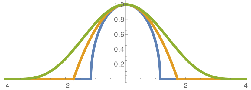
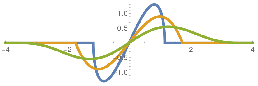
Figure 2.1: The left figure shows the Barenblatt profiles $W$ for $m=1.25$ (green), $m=2$, and $m=3$ (blue). The right picture shows the corresponding self-similar flux pattern $Q$.

To emphasize that $W$ is a non-equilibrium steady state (NESS), we look at the mass fluxes. In (2.1) we have the diffusive flux $q(t,x)=-(u^{m})_{x}$ and the total mass $M=\int_{\mathbb{R}}u(t,x)\;\!\mathrm{d}x$ is preserved for solutions $u$. Indeed, the flux $q=-(u^{m})_{x}$ takes the form $q(t,x)=(1{+}t)^{-m\alpha-\beta}Q(x/(1{+}t)^{\beta})$ with similarity profile

$$Q(y)=-\big{(}W^{m}\big{)}_{y}(y)=-m\,W(y)^{m-1}W^{\prime}(y).$$

2.2 Diffusive mixing and infiltration

We may also consider PME with boundary conditions $u(t,\pm\infty)=U_{\pm}$ with different concentrations $U_{-}$ and $U_{+}$. Again a self-similar profile develops but now the scaling is different as $u$ cannot be scaled by a prefactor, because of the boundary conditions. The boundary conditions provide reservoirs with an infinite amount of mass at $x=+\infty$ and $x=-\infty$. The diffusive mixing describes how the mass is flowing from one reservoir to the other.

In particular, we have to choose $\alpha=0$ and are then forced to take $\beta=1/2$, which is the parabolic scaling. The corresponding equation in the parabolic similarity coordinates reads

$$w_{\tau}=(w^{m})_{yy}+\frac{y}{2}\,w_{y},\quad w(\tau,\pm\infty)=U_{\pm}.$$ (2.3)

Of course steady states $W$ are again exact self-similar solutions to (2.3). The existence and uniqueness of stationary profiles $W$ with $W(\pm\infty)=U_{\pm}$ are studied in [MiS23]. The profiles are monotone and converge to their limits $U_{\pm}$ faster than exponential. For $U_{-}>U_{+}$ the flux is nonnegative and has its maximum at $y=0$, see Figure 2.2. The diffusive flux $q=-(u^{m})_{x}$ scales differently from before, but the self-similar profile $Q$ has the same expression as before:

$$q(t,x)=-(1{+}t)^{-1/2}Q\big{(}x/(1{+}t)^{1/2}\big{)}\ \text{ with }$$

$$Q(y)=-\big{(}W^{m}\big{)}^{\prime}(y)=-mW(y)^{m-1}W^{\prime}(y).$$

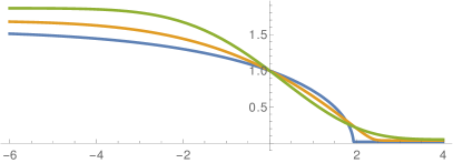
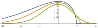
Figure 2.2: The left figure shows the self-similar infiltration profiles with $U_{+}=0$ and $W(0)=1$ for $m=1.25$ (green), $m=2$, and $m=3$ (blue). The right picture shows the corresponding flux $Q$.

The case $U_{+}=0$ is called the case of filtration, where mass is flowing into the area $x\gg 1$ where initially the concentration is $0$. For all $m>1$ the front propagates like $t^{1/2}$ and the infiltrated mass given by $M_{\geq}(t)=\int_{0}^{\infty}u(t,x)\;\!\mathrm{d}x$ satisfies $\dot{M}_{\geq}(t)=q(t,0)=(1{+}t)^{-1/2}Q(0)$, i.e. we have $M_{\geq}(t)=M_{\geq}(0)(1{+}t)^{1/2}$.

3 A model motivated by turbulence

Kolmogorov’s two-equation model [Kol42, Spa91, BuM19] considered on all of ${\mathbb{R}}^{d}$ has a rich scaling structure and hence allows for self-similar solutions, see Sec. 3 in [MiN22]. In [Mie22] a simplified model is studied, where $\widetilde{v}(t,x)$ is a scalar shear velocity and $\widetilde{k}(t,x)$ is the mean turbulent kinetic energy:

$$\widetilde{v}_{t} =\mathop{\mathrm{div}}\nolimits\big{(}\eta\,\widetilde{k}^{\beta}\nabla v\big{)},$$

$$\widetilde{k}_{t} =\mathop{\mathrm{div}}\nolimits\big{(}\kappa\,\widetilde{k}^{\beta}\nabla\widetilde{k}\big{)}+\eta\widetilde{k}^{\alpha}|\nabla\widetilde{v}|^{2},$$

where $\eta,\kappa,\beta$ are positive parameters. Note that the system contains the PME with $m=\beta+1$, if we look at the case $\widetilde{v}\equiv 0$.

The system has the total linear momentum ${\mathcal{P}}(\widetilde{v})=\int_{{\mathbb{R}}^{d}}\widetilde{v}(x)\;\!\mathrm{d}x$ and the total energy ${\mathcal{E}}(\widetilde{v},k)=\int_{{\mathbb{R}}^{d}}\big{(}\frac{1}{2}\widetilde{v}^{2}+\widetilde{k}\big{)}\;\!\mathrm{d}x$ as conserved quantities. The kinetic energy that is dissipated via shear viscosity (depending on $\widetilde{k}$) is fully fed into the turbulent kinetic energy, which leads to the energy conservation.

In fact, the system can be written as a gradient-flow equation with respect to entropy ${\mathcal{S}}(\widetilde{k})=\int_{{\mathbb{R}}^{d}}\widetilde{k}^{\theta}\;\!\mathrm{d}x$ for any $\theta\in(0,1)$, hence it is expected that $\widetilde{k}$ has to become constant. For bounded domains with no-flux boundary conditions, it can be shown that solutions converge exponentially to the unique equilibrium state with constant $\widetilde{v}$ and $\widetilde{k}$ such that the conserved quantities match, see Sec. 2 in [Mie22].

On the unbounded domain ${\mathbb{R}}^{d}$, solutions with finite momentum ${\mathcal{P}}$ and finite energy ${\mathcal{E}}$ are expected to disperse and converge uniformly to $0$. In Sec. 6 of [Mie22] it is argued that $\widetilde{v}$ and $\widetilde{k}$ behave asymptotically self-similar, but with different exponents because of $\frac{1}{2}\widetilde{v}^{2}$ in the energy and $\widetilde{v}$ in the momentum. The conjecture is that $\widetilde{k}$ develops, for large $t$, a self-similar pattern of Barenblatt type, namely

$$K(y)=\max\{0,N-c_{\beta+1}|y|^{2}\}^{1/\beta}$$ (3.1)

with total mass $E={\mathcal{E}}(v(0),k(0))$, which means that all macroscopic kinetic energy is converted into turbulent kinetic energy. Moreover, $\widetilde{v}$ develops, for large $t$, a self-similar pattern that is a Barenblatt solution raised to the power $\kappa/\eta$, i.e.

$$V(y)=\widetilde{v}\,\big{(}K(y)\big{)}^{\kappa/\eta}$$

with $\widetilde{v}$ such that ${\mathcal{P}}(V)={\mathcal{P}}(v(0))$.

More precisely, with $\gamma=1/(2{+}\beta d)$ we rescale the variables via

$$\tau=\log(1{+}t),\ y=x/(1{+}t)^{\gamma},\ k=(1{+}t)^{\gamma d}\widetilde{k},\ v=(1{+}t)^{\gamma d}\widetilde{v}$$

and obtain a non-autonomous coupled system

$$v_{\tau} =\mathop{\mathrm{div}}\nolimits\big{(}\gamma vy+\eta\,k^{\beta}\nabla v\big{)},$$

$$k_{\tau} =\mathop{\mathrm{div}}\nolimits\big{(}\gamma ky+\kappa\,k^{\beta}\nabla k\big{)}+\mathrm{e}^{-\gamma d\tau}\,\eta k^{\beta}|\nabla v|^{2},$$

where now $\mathop{\mathrm{div}}\nolimits$ and $\nabla$ are taken with respect to $y$. Thus, we see that the equation for $k$ behaves, for $\tau\gg 1$, like the PME and has the Barenblatt profiles from (3.1) as asymptotic steady states. Inserting such a Barenblatt solution $K$, one can show that the linear equation for $V$ has the steady states $\widetilde{v}K^{\kappa/\eta}$. For $\eta\gg\kappa$, this means that $V$ will have large gradients near the boundary of the support of $K$.

As for the PME equation there are also solutions with infinite momentum or energy, because there are nontrivial limits at $x\to\pm\infty$. In one such case it is possible to write down an exact self-similar solution, namely for $\alpha=\beta=1$ and $\kappa=\eta$, where we set $\eta=1$ for simplicity. With $y=x/\sqrt{1{+}t}$ and arbitrary $A>0$ it can be checked that $v(t,x)=V(y)$ and $k(t,x)=K(y)$ are explicit solutions, if we choose

$$\big{(}V(y),K(y)\big{)}=\left\{\begin{array}[]{@{}cl}\big{(}A/\sqrt{2},0\big{)}&\text{for }y\geq A,\\ \big{(}y/\sqrt{2},(A^{2}{-}y^{2})/4\big{)}&\text{for }|y|\leq A,\\ \big{(}-A/\sqrt{2},0\big{)}&\text{for }y\leq-A.\end{array}\right.$$

For this solution, the energy density $e(t,x)=\frac{1}{2}v(t,x)^{2}+k(t,x)$ is indeed equal to the constant $A^{2}/4$, which means that the solutions have infinite total energy. Nevertheless there are nontrivial fluxes, namely for the linear momentum and the turbulent kinetic energy:

$$Q^{\mathrm{lin.mom}}(y)=-K(y)V^{\prime}(y)=-K(y)/\sqrt{2},$$

$$Q^{\mathrm{tur.kin}}(y)=-K(y)K^{\prime}(y),\text{ and}$$

$$S^{\mathrm{tur.kin}}(y)=K(y)V^{\prime}(y)^{2}=K(y)/2\geq 0,$$

where the last term is the source of turbulent kinetic energy stemming from the dissipation in the momentum equation.

4 Diffusive mixing in reaction-diffusion systems

Here we consider systems of equations which describe the concentrations $c_{j}$ of species $X_{j}$ that diffuse with a diffusion constant $d_{j}$ and that undergo reactions according to the mass-action law. Our main assumption is that there is a continuous family of equilibria to the reaction equation $\dot{\bm{c}}={\bm{R}}({\bm{c}})$, where ${\bm{c}}=(c_{1},...,c_{i_{*}})\in\mathfrak{C}:={[0,\infty[}^{i_{*}}$ is the vector of concentration. We consider the reaction-diffusion system (RDS) on the real line ${\mathbb{R}}^{1}$ and impose boundaries conditions at infinity which represent reservoirs of infinite mass. The prescribed limit states $C_{-}$ and $C_{+}$ at $x=\pm\infty$ are assumed to be in equilibrium, i.e. ${\bm{R}}(C_{\pm})=0$. Thus, our RDS takes the form

$$\widetilde{\bm{c}}_{t}={\bm{D}}\,\widetilde{\bm{c}}_{xx}+{\bm{R}}(\widetilde{\bm{c}}),\quad\widetilde{\bm{c}}(t,\pm\infty)=C_{\pm},$$ (4.1)

where ${\bm{D}}$ is the diagonal matrix $\mathrm{diag}(d_{1},...,d_{i_{*}})$.

To study self-similar behavior, we use the parabolic scaling variables $\tau=\log(1{+}t)$ and $y=x/\sqrt{1{+}t}$ again and find for ${\bm{c}}(\tau,y)=\widetilde{\bm{c}}(t,x)$ the scaled equations

$${\bm{c}}_{\tau}={\bm{D}}\,{\bm{c}}_{yy}+\frac{y}{2}\,{\bm{c}}+\mathrm{e}^{\tau}\,{\bm{R}}({\bm{c}}),\quad{\bm{c}}(\tau,\pm\infty)=C_{\pm},$$ (4.2)

where the prefactor $\mathrm{e}^{\tau}$ appears because the reactions do not scale in a similar way as the derivatives $\partial_{\tau}$ and $\partial_{y}^{2}$.

Hence, for large $\tau$ the reaction becomes stronger and stronger and will lead to a local equilibration of the reactions. Of course, this is only an effect of the scaling, but it says that on long time scales we first see that the reactions act on their natural time scale while the diffusive mixing may take much longer and will actually never stop because of the boundary conditions at $\pm\infty$.

4.1 The diffusive large-time limit and reduced systems

We can formally go to the limit $\tau\gg 1$ in (4.2) as follows. Clearly, the reaction has to become equilibrated, i.e. ${\bm{R}}({\bm{c}}(\tau,y))=\bm{0}$ for all $\tau$ and $y$. However, the product $\mathrm{e}^{\tau}{\bm{R}}({\bm{c}})$ should then be treated as a limit of the type “$\infty\cdot\bm{0}$”, taking the value ${\bm{\lambda}}(\tau,y)\in{\mathbb{R}}^{i_{*}}$. This term can be understood as a rescaled version of a small reaction flux, because the reaction ${\bm{c}}$ will only be equilibrated up to order $\mathrm{e}^{-\tau}$ such that ${\bm{R}}({\bm{c}})$ may still contain a term $\mathrm{e}^{-\tau}{\bm{\lambda}}$.

The models resulting from (4.1) and (4.2) are the following constrained RDS

$$\widetilde{\bm{c}}_{\tau} ={\bm{D}}\,\widetilde{\bm{c}}_{xx}+\widetilde{\bm{\lambda}},\quad{\bm{R}}(\widetilde{\bm{c}})=0,\quad\widetilde{\bm{c}}(t,\pm\infty)=C_{\pm},$$ (4.3a)

$${\bm{c}}_{\tau} ={\bm{D}}\,{\bm{c}}_{yy}+\frac{y}{2}\,{\bm{c}}_{y}+{\bm{\lambda}},\quad{\bm{R}}({\bm{c}})=0,\quad{\bm{c}}(\tau,\pm\infty)=C_{\pm}.$$ (4.3b)

The important point is that ${\bm{\lambda}}$ is restricted to lie in the linear subspace $\mathrm{span}\big{\{}\,{\mathrm{D}}{\bm{R}}({\bm{c}}){\bm{v}}\>\big{|}\>{\bm{R}}({\bm{c}})=0,\ {\bm{v}}\in{\mathbb{R}}^{i_{*}}\,\big{\}}$, such that ${\bm{\lambda}}$ plays the role of a Lagrange multiplier to the constraint ${\bm{R}}({\bm{c}})=\bm{0}$.

We restrict to the case of mass-action kinetics, where the reaction is in detailed balance. Then, there exists a surjective linear stoichiometric mapping ${\bm{Q}}:{\mathbb{R}}^{i_{*}}\to{\mathbb{R}}^{j_{*}}$ giving the conserved molecular masses and a nonlinear map $\Psi:\;\mathfrak{U}:={\bm{Q}}\mathfrak{C}\to\mathfrak{C}$ such that

$${\bm{Q}}{\bm{R}}({\bm{c}})=0\text{ for all }{\bm{c}}\in\mathfrak{C},\quad{\bm{Q}}\Psi({\bm{u}})={\bm{u}}\text{ for all }{\bm{u}}\in\mathfrak{U},$$

$$\text{and }\big{\{}\,{\bm{c}}\in\mathfrak{C}\>\big{|}\>{\bm{R}}({\bm{c}})=0\,\big{\}}=\big{\{}\,\psi({\bm{u}})\in\mathfrak{C}\>\big{|}\>{\bm{u}}\in\mathfrak{U}\,\big{\}},$$

i.e. $\Psi$ parametrizes the set of equilibria of ${\bm{R}}$. We refer to [MPS21, MiS22] for more details.

Setting $\widetilde{\bm{u}}(t,x)={\bm{Q}}\widetilde{\bm{c}}(t,x)$, ${\bm{u}}(\tau,y)={\bm{Q}}{\bm{c}}(\tau,y)$, and $U_{\pm}={\bm{Q}}C_{\pm}$, the constrained RDS (4.3) in unscaled and scaled form reduce to the simple diffusion systems

$$\widetilde{\bm{u}}_{t} =\big{(}{\bm{A}}(\widetilde{\bm{u}})\big{)}_{xx},\quad{\bm{u}}(t,\pm\infty)=U_{\pm}\quad\text{and}$$ (4.4a)

$${\bm{u}}_{\tau} =\big{(}{\bm{A}}({\bm{u}})\big{)}_{yy}+\frac{y}{2}\,{\bm{u}}_{y},\quad{\bm{u}}(\tau,\pm\infty)=U_{\pm}$$ (4.4b)

with ${\bm{A}}({\bm{u}})={\bm{Q}}\,{\bm{D}}\,\Psi({\bm{u}})$. Note that ${\bm{Q}}{\bm{\lambda}}\equiv 0$ by construction.

4.2 Vector-valued profile equations

Under the assumption that ${\bm{A}}:{\mathbb{R}}^{j_{*}}\to{\mathbb{R}}^{j_{*}}$ is (strongly) monotone, the vector-valued profile equation

$$\bm{0}=\big{(}{\bm{A}}({\bm{U}})\big{)}_{yy}+\frac{y}{2}\,{\bm{U}}_{y},\quad{\bm{U}}(\pm\infty)=U_{\pm}$$ (4.5)

has a unique similarity profile ${\bm{U}}:{\mathbb{R}}\to{\mathbb{R}}^{j_{*}}$. We refer to [GaM98] for the scalar-valued case and to [MiS23] for the more general vector-valued case.

A profile ${\bm{U}}$ solving (4.5) is a classical steady state solution for the scaled diffusion system (4.4b). Hence, setting $\widetilde{u}(t,x)={\bm{U}}\big{(}x/\sqrt{1{+}t}\big{)}$ provides an exact self-similar solution to (4.4a).

Clearly, defining ${\bm{C}}(y)=\Psi({\bm{U}}(y))$ we obtain a solution ${\bm{C}}:{\mathbb{R}}\to{\mathbb{R}}^{i_{*}}$ for the constrained profile equation

$$\bm{0}={\bm{D}}{\bm{C}}_{yy}+\frac{y}{2}\,{\bm{C}}_{y}+{\bm{\lambda}},\quad{\bm{R}}({\bm{C}})=\bm{0},$$ (4.6)

$${\bm{Q}}{\bm{\lambda}}=0,\quad{\bm{C}}(\pm\infty)=\Psi(U_{\pm}).$$

The similarity profile ${\bm{C}}$ is a steady state for the scaled constrained RDS (4.3b), and $\widetilde{\bm{c}}(t,x)={\bm{C}}\big{(}x/\sqrt{1{+}t}\big{)}$ is an exact self-similar solution for (4.3a).

In the following three subsections, we consider a few special cases, where we highlight the role of the reaction flux(es) ${\bm{\lambda}}$ in particular.

4.3 One reaction for two species

In [GaS22, MiS22] the following system of two equations is studied in detail:

$$\binom{\dot{c}_{1}}{\dot{c}_{2}}=\binom{d_{1}\,\partial_{x}^{2}c_{1}}{d_{2}\,\partial_{x}^{2}c_{2}}+\kappa\big{(}c_{2}^{\beta}{-}c_{1}^{\gamma}\big{)}\binom{\gamma}{-\beta}\qquad\text{for }t>0\text{ and }x\in{\mathbb{R}}.$$

The two concentrations $c_{1},c_{2}\geq 0$ for the species $X_{1},X_{2}$ diffusive with diffusion constants $d_{j}$ and undergo the reversible mass-action reaction pair $\gamma X_{1}\rightleftharpoons\beta X_{2}$.

The scaled and constraint system (4.3b) takes the form

$$\partial_{\tau}\!\binom{c_{1}}{c_{2}}=\binom{d_{1}\,\partial_{y}^{2}c_{1}}{d_{2}\,\partial_{y}^{2}c_{2}}+\frac{y}{2}\partial_{y}\!\binom{c_{1}}{c_{2}}+\Lambda\binom{\gamma}{\!\!-\beta\!\!},\ \ \Lambda\in{\mathbb{R}},\ \ c_{1}^{\gamma}=c_{2}^{\beta}.$$

Here ${\bm{\lambda}}=\Lambda(\gamma,-\beta)^{\top}\in{\mathbb{R}}^{2}$ contains only one scalar reaction flux $\Lambda\in{\mathbb{R}}$, because there is only one reaction pair.

The set of equilibria for ${\bm{R}}$ is the one-parameter family

$$\big{\{}\,{\bm{c}}\in\mathfrak{C}\>\big{|}\>{\bm{R}}({\bm{c}})=0\,\big{\}}=\big{\{}\,(A^{\beta},A^{\gamma})\>\big{|}\>A\geq 0\,\big{\}}.$$

The linear stoichiometric mapping is ${\bm{Q}}=\big{(}\beta\ \ \gamma\big{)}\in{\mathbb{R}}^{1\times 2}$ defining $u={\bm{Q}}{\bm{c}}=\beta c_{1}{+}\gamma c_{2}\geq 0$, and $\Psi:{[0,\infty[}=\mathfrak{U}\to\mathfrak{C}$ is defined via

$${\bm{c}}=\Psi(u)=\binom{\psi_{1}(u)}{\psi_{2}(u)}\quad\Longleftrightarrow\quad\left\{\begin{array}[]{c}u={\bm{Q}}{\bm{c}}=\beta c_{1}{+}\gamma c_{2}\\ \text{and }c_{1}^{\gamma}=c_{2}^{\beta}\end{array}\right.$$

The case $\gamma=\beta$ leads to the simple relation $\Psi(u)=\frac{1}{\beta{+}\gamma}\binom{u}{u}$. If $\beta\neq\gamma$ we may assume $\beta<\gamma$ without loss of generality, see (4.8) for a nontrivial example.

For $A_{\Psi}(u):={\bm{Q}}{\bm{D}}\Psi(u)=\binom{\beta d_{1}}{\gamma d_{2}}\bm{\cdot}\Psi(u)$ one obtains $0<\psi^{\prime}_{1}(u)\leq\psi^{\prime}_{1}(0)=1/\beta$ and $0<\psi^{\prime}_{2}(u)\leq\psi^{\prime}_{2}(\infty)=1/\gamma$. This yields

$$D_{*}=\min\{d_{1},d_{2}\}\leq A^{\prime}_{\Psi}(u)\leq D^{*}=\max\{d_{1},d_{2}\}$$

as well as $A^{\prime}_{\Psi}(u)\to d_{1}$ for $u\to 0^{+}$ and $A^{\prime}_{\Psi}(u)\to d_{2}$ for $u\to\infty$.

Thus, the existence theory for similarity profiles in [GaM98, MiS23] provides a unique and smooth solution $U$ of the profile equation

$$\big{(}A_{\Psi}(U)\big{)}^{\prime\prime}+\frac{y}{2}\,U^{\prime}=0\ \text{ on }{\mathbb{R}},\quad U(\pm\infty)=U_{\pm}.$$

Assuming $U_{-}<U_{+}$, this solution is strictly increasing and converges to its two limits like the error function. In addition to $U_{-}<U(y)<U_{+}$ the estimate

$$0<U^{\prime}(y)\leq\mathrm{e}^{-y^{2}/(4D^{*})}\sqrt{\tfrac{\displaystyle D^{*}}{\displaystyle 8D_{*}^{2}}}\,\big{(}U_{+}-U_{-}\big{)}\quad\text{for all }y\in{\mathbb{R}}$$ (4.7)

holds, even in the case $U_{-}=0$, where asymptotically the concentrations vanish, viz. $C_{-}=\Psi(U_{-})=\binom{0}{0}$, because the effective diffusion is still bounded from below by $D_{*}>0$.

Such a profile $U:{\mathbb{R}}\to[U_{-},U_{+}]$ for the reduced equation leads to a smooth concentration profile ${\bm{C}}:{\mathbb{R}}\to\mathfrak{C}\subset{\mathbb{R}}^{2}$ given by ${\bm{C}}(y)=\Psi(U(y))$ and satisfying the profile equation

$$0=\left(\begin{array}[]{@{}c@{}c@{}}d_{1}&0\\ 0&d_{2}\end{array}\right){\bm{C}}^{\prime\prime}+\frac{y}{2}\,{\bm{C}}^{\prime}+\Lambda\binom{\gamma}{-\beta},\quad C_{1}^{\gamma}=C_{2}^{\beta},$$

$${\bm{C}}(y)\to\Psi(U_{\pm})\text{ for }y\to\pm\infty.$$

Hence, the reaction flux $\Lambda$ can be written as

$$\Lambda(y):=-\frac{1}{\gamma}\big{(}d_{1}C^{\prime\prime}_{1}(y)+\frac{y}{2}C^{\prime}_{1}(y)\big{)}=\frac{1}{\beta}\big{(}d_{2}C^{\prime\prime}_{2}(y)+\frac{y}{2}C^{\prime}_{2}(y)\big{)}.$$

In general, $\Lambda$ will be nontrivial, this can already be seen in the simple case $\beta=\gamma$, which implies $C_{1}\equiv C_{2}$, $\psi_{j}(u)=u/(\beta{+}\gamma)$, and hence $A_{\Psi}(u)=\frac{d_{1}{+}d_{2}}{2}u$. Denoting by ${\mathbb{E}}:{\mathbb{R}}\to{]0,1[}$ the unique solution of ${\mathbb{E}}^{\prime\prime}+y{\mathbb{E}}^{\prime}=0$, ${\mathbb{E}}(-\infty)=0$, and ${\mathbb{E}}(\infty)=1$ and recalling $U_{\pm}=2\gamma C_{\pm}$, we obtain the unique profiles

$$U(y) =2\gamma C_{-}+2\gamma(C_{+}{-}C_{-}){\mathbb{E}}\big{(}y/(d_{1}{+}d_{2})\big{)},$$

$$C_{1}(y) =C_{2}(y)=\frac{1}{2\gamma}\,U(y).$$

This provide the explicit formula (for $\beta=\gamma$ only), namely

$$\Lambda(y)=\frac{2(d_{1}{-}d_{2})}{(d_{1}{+}d_{2})^{2}}\,\big{(}C_{+}-C_{-}\big{)}\>{\mathbb{E}}^{\prime\prime}\big{(}y/(d_{1}{+}d_{2})\big{)},$$

i.e. only for $d_{1}=d_{2}$ we have $\Lambda\equiv 0$.

Figure 4.1: For the case $\beta=\gamma=1$ the similarity profile $C_{1}=C_{2}$ is shown together with the diffusive fluxes $Q_{j}^{\mathrm{react}}$ and the reaction flux $\Lambda^{\mathrm{react}}$.

In Figure 4.1 we display, for $C_{-}=0.2<C_{+}=1.2$, $\beta=\gamma=1$, and $d_{1}=1>d_{2}=0.5$, the profile $C_{1}=C_{2}$, the associated diffusion fluxes $Q^{\text{diff}}_{j}=-d_{j}C^{\prime}_{j}(y)$ for $j=1,2$, and the reaction flux $\Lambda^{\mathrm{react}}$. Because of the $d_{1}>d_{2}$ the diffusive fluxes satisfy $|Q^{\text{diff}}_{1}|>|Q^{\text{diff}}_{2}|$, so one would expect the profile $C_{1}$ to be flatter than $C_{2}$. However, $C_{1}=C_{2}$ is realized by the reaction $X_{1}\rightleftharpoons X_{2}$, which pushes missing or excessive mass from $X_{1}$ into $X_{2}$.

We also consider the case $\beta=1$ and $\gamma=2$ which corresponds to the nonlinear reaction pair $X_{1}\rightleftharpoons 2X_{2}$. Now, the profiles are no longer identical and there is no symmetry $y\leftrightarrow-y$. We find

$$\Psi(u)=\binom{\frac{1}{4}\big{(}\sqrt{1{+}8u}-1\big{)}}{\frac{1}{8}\big{(}1+4u-\sqrt{1{+}8u}\big{)}},$$ (4.8)

and can calculate all fluxes for $C_{-}=\Psi(1)=\binom{1/2}{1/4}$ and $C_{-}=\Psi(6)=\binom{3/2}{9/4}$, now choosing $d_{1}=1$ and $d_{2}=1$ which gives $A_{\Psi}(u)=u$ and makes the calculation simple. We refer to Figure 4.2 for the corresponding profiles and diffusion and reaction fluxes.

Figure 4.2: For the case $\beta=1<\gamma=2$ and $d_{1}=d_{2}=1$ the similarity profile $C_{1}$ and $C_{2}$ are shown (left picture) and the associated diffusion fluxes and reaction flux (right picture).

4.4 One reaction for three species

For the typical binary reaction $X_{3}\rightleftharpoons X_{1}{+}X_{2}$ we obtain the scaled constrained RDS

$$\partial_{\tau}{\bm{c}}={\bm{D}}\partial_{y}^{2}{\bm{c}}+\frac{y}{2}\partial_{y}{\bm{c}}+\Lambda\!\left(\begin{array}[]{@{}c@{}}1\\[-1.00006pt] 1\\[-1.00006pt] -1\end{array}\right)\!,\quad c_{1}c_{2}=c_{3}$$

with ${\bm{D}}=\mathrm{diag}(d_{1},d_{2},d_{3})$. The profile equation reads

$$0 ={\bm{D}}{\bm{C}}^{\prime\prime}+\frac{y}{2}{\bm{C}}^{\prime}+\Lambda\!\left(\begin{array}[]{@{}c@{}}1\\[-1.00006pt] 1\\[-1.00006pt] -1\end{array}\right)\!,\quad C_{1}C_{2}=C_{3}\quad\text{and}\ \ {\bm{C}}(\pm\infty)=\Psi({\bm{U}}_{\pm}).$$ (4.9)

The set of equilibria for ${\bm{R}}$ is a two-parameter family:

$$\big{\{}\,{\bm{c}}\in\mathfrak{C}\>\big{|}\>{\bm{R}}({\bm{c}})=0\,\big{\}}=\big{\{}\,(A,B,AB)\>\big{|}\>A,B\geq 0\,\big{\}}.$$

We can choose the stoichiometric matrix

$${\bm{Q}}=\left(\begin{array}[]{ccc}1&0&1\\ 0&1&1\end{array}\right)\in{\mathbb{R}}^{2\times 3}$$

and obtain ${\bm{u}}=\binom{u_{1}}{u_{2}}={\bm{Q}}{\bm{c}}\in\mathfrak{U}:={[0,\infty[}^{2}$. The reduction function $\Psi:\mathfrak{U}\to\mathfrak{C}$ can be calculated explicitly in the form

$$\Psi(u_{1},u_{2}) =\frac{1}{2}\!\left(\begin{array}[]{@{}c@{}}u_{1}{-}u_{2}{-}1+s({\bm{u}})\\[-1.00006pt] u_{2}{-}u_{1}{-}1+s({\bm{u}})\\[-1.00006pt] u_{1}{+}u_{2}{+}1-s({\bm{u}})\end{array}\right)\!\quad\text{with}s({\bm{u}})=\sqrt{(1{+}u_{1}{+}u_{2})^{2}-4u_{1}u_{2}}.$$

To extend $s$ to a function $s:{\mathbb{R}}^{2}\to{\mathbb{R}}$ we simply set $s(u_{1},u_{2})=1+u_{1}+u_{2}$ whenever $u_{1}\leq 0$ or $u_{2}\leq 0$ and observe that $s$ is globally Lipschitz continuous. Moreover, $s_{j}({\bm{u}})=\partial_{u_{j}}s({\bm{u}})$ satisfies $s_{1}({\bm{u}})\leq 1$, $s_{2}({\bm{u}})\leq 1$ and $s_{1}({\bm{u}})+s_{2}({\bm{u}})\geq 0$ for all ${\bm{u}}\in{\mathbb{R}}^{2}$.

From this we can calculate the function ${\bm{A}}({\bm{u}})={\bm{Q}}\,{\bm{D}}\,\Psi({\bm{u}})$:

$${\bm{A}}({\bm{u}})=\frac{1}{2}\binom{(d_{1}{+}d_{3})u_{1}+(d_{3}{-}d_{1})(1{+}u_{2}{-}s({\bm{u}}))}{(d_{2}{+}d_{3})u_{2}+(d_{3}{-}d_{2})(1{+}u_{1}{-}s({\bm{u}}))}.$$

To show monotonicity of ${\bm{A}}:{\mathbb{R}}^{2}\to{\mathbb{R}}^{2}$ we observe that for general ${\mathrm{C}}^{1}$ functions ${\bm{A}}$ we have the equivalence

$$\forall\,{\bm{u}},\widetilde{\bm{u}}:\ \langle{\bm{A}}({\bm{u}}){-}{\bm{A}}(\widetilde{\bm{u}}),{\bm{u}}{-}\widetilde{\bm{u}}\rangle\geq{\mathrm{a}}_{{\mathrm{l}}{\mathrm{o}}}|{\bm{u}}{-}\widetilde{\bm{u}}|^{2}$$

$$\Longleftrightarrow\quad\forall\,{\bm{u}}:\ \frac{1}{2}\big{(}{\mathrm{D}}{\bm{A}}({\bm{u}}){+}{\mathrm{D}}{\bm{A}}({\bm{u}})^{\top}\big{)}\geq{\mathrm{a}}_{{\mathrm{l}}{\mathrm{o}}}I_{m\times m}.$$

Using this, it is shown in [MiS23] that ${\bm{A}}$ is monotone if and only if

$$(3{-}\sqrt{8}\,)d_{3}<d_{j}<(3{+}\sqrt{8}\,)d_{3}\quad\text{ for }j=1,\ 2.$$

Hence, the vector-valued version of the existence theorem for similarity profiles can be applied and for all limits ${\bm{U}}_{-}$ and ${\bm{U}}_{+}$ there exists a unique similarity profile ${\bm{U}}:{\mathbb{R}}\to{\mathbb{R}}^{2}$ connecting ${\bm{U}}_{-}$ and ${\bm{U}}_{+}$. These solutions give rise to similarity profiles ${\bm{C}}=\Psi{\circ}{\bm{U}}$ connecting $\Psi({\bm{U}}_{-})$ and $\Psi({\bm{U}}_{+})$ if and only if ${\bm{U}}(y)\in\mathfrak{U}={[0,\infty[}^{2}$ for all $y\in{\mathbb{R}}$, thus providing ${\bm{C}}(y)=\Psi({\bm{U}}(y))\in\mathfrak{C}={[0,\infty[}^{3}$. In general, it seems to be difficult to guarantee this condition, but defining $\overline{\bm{u}}_{(\pm)}:{\mathbb{R}}\to{\mathbb{R}}^{2}$ via

$$\overline{\bm{u}}_{(\pm)}(y)={\bm{U}}_{\pm}\text{ for }\pm y>0\text{ and }\overline{\bm{u}}_{(\pm)}(0)=\frac{1}{2}({\bm{U}}_{-}{+}{\bm{U}}_{+}),$$

one can show the uniform estimate

$$\big{|}{\bm{U}}(y)-\overline{\bm{u}}_{(\pm)}(y)\big{|}\leq C_{*}|{\bm{U}}_{+}{-}{\bm{U}}_{-}|,$$

where $C_{*}$ only depends on $d_{1}$, $d_{2}$, and $d_{3}$, but not on ${\bm{U}}_{\pm}$. Thus, we obtain valid similarity profiles if $|{\bm{U}}_{+}{-}{\bm{U}}_{-}|$ is sufficiently small compared to the distance of ${\bm{U}}_{+}$ and ${\bm{U}}_{-}$ from the boundary of $\mathfrak{U}$. In that case, similarity profiles ${\bm{C}}:{\mathbb{R}}\to{\mathbb{R}}^{3}$ solving (4.9) exist and are unique.

In the present example we obtain nonmonotone profiles ${\bm{C}}:{\mathbb{R}}\to\mathfrak{C}\subset{\mathbb{R}}^{3}$. For this, consider the case $d_{1}=d_{2}$ and the limits

$$C_{-}=(A,B,AB)^{\top}\quad\text{and}\quad C_{+}=(B,A,AB)^{\top}\quad\text{ with }A\neq B.$$

Our uniqueness result and the reflection symmetries $x\to-x$ and $(c_{1},c_{2})\to(c_{2},c_{1})$ imply that the stationary profile ${\bm{C}}$ satisfies $C_{1}(y)=C_{2}(-y)$ and $C_{3}(y)=C_{3}(-y)$. Using $C_{1}(y)C_{2}(y)=C_{3}(y)$ for all $y\in{\mathbb{R}}$ we see that $C_{3}$ cannot be constant, hence it must be nonmonotone. Figure 4.3 shows a corresponding example.

Figure 4.3: Solution ${\bm{C}}=(C_{1}(y),C_{2}(y),C_{3}(y))$ of (4.9) for $d_{1}=d_{2}=2$ and $d_{3}=10$ with limiting values $C_{-}\approx(5.3,0.3,1.6)$ and $C_{+}\approx(0.3,5.3,1.6)$. This symmetric solution was obtained by starting with ${\bm{C}}(0)=(1.5,1.5,2.25)$ and ${\bm{C}}^{\prime}(y)=(-1,1,0)$.

An interesting question is whether there is a stationary profile ${\bm{C}}$ connecting the limiting cases

$$C_{-}=\Psi(1,0)=(1,0,0)^{\top}\quad\text{and}\quad C_{-}=\Psi(0,1)=(0,1,0)^{\top}.$$

The profile would see only one of the species $X_{1}$ or $X_{2}$ in the reservoirs at $\pm\infty$, however in the middle region all three species must be present to allow the generation of the other species.

4.5 Two reactions for three species

Consider the two reactions $2X_{1}\leftrightharpoons X_{2}$ and $X_{2}\leftrightharpoons X_{3}$ giving

$$\partial_{\tau}{\bm{c}}={\bm{D}}\partial_{y}^{2}{\bm{c}}-k_{1}\big{(}c_{1}^{2}-c_{2}\big{)}\!\left(\begin{array}[]{@{}c@{}}2\\[-1.00006pt] -1\\[-1.00006pt] 0\end{array}\right)\!-k_{2}\big{(}c_{2}-c_{3}\big{)}\!\left(\begin{array}[]{@{}c@{}}0\\[-1.00006pt] 1\\[-1.00006pt] -1\end{array}\right)\!.$$ (4.10)

The set of equilibria is the one-parameter family given by

$$\big{\{}\,{\bm{c}}\in\mathfrak{C}\>\big{|}\>{\bm{R}}({\bm{c}})=0\,\big{\}}=\big{\{}\,(A,A^{2},A^{2})\>\big{|}\>A\geq 0\,\big{\}}.$$

Note that the RDS system has invariant regions of the form $\Sigma:=[b,B]\times[b^{2},B^{2}]\times[b^{2},B^{2}]$ for arbitrary $0\leq b<B<\infty$. This means that any solution satisfying ${\bm{c}}(0,x)\in\Sigma$ for all $x\in{\mathbb{R}}$ also satisfies ${\bm{c}}(t,x)\in\Sigma$ for all $t>0$ and $x\in{\mathbb{R}}$, see [Smo94] for the theory of invariant regions for RDS. Thus, a similarity profile connecting $C_{-}=(b,b^{2},b^{2})$ and $C_{+}=(B,B^{2},B^{2})$ is expected to lie in the invariant region $\Sigma$.

The stoichiometric matrix is ${\bm{Q}}=(1\ \ 2\ \ 2)\in{\mathbb{R}}^{1\times 3}$ and

$$u={\bm{Q}}{\bm{c}}=c_{1}{+}2c_{2}{+}2c_{3}\ \text{ yields }\ \Psi(u)=\!\left(\begin{array}[]{@{}c@{}}\sigma(u)\\[-1.00006pt] (u{-}\sigma(u))/4\\[-1.00006pt] (u{-}\sigma(u))/4\end{array}\right)\!$$

with $\sigma(u)=(\sqrt{1{+}16\,u}-1)/8$. With $\sigma^{\prime}(u)=1/\sqrt{1{+}16\,u}\in[0,1]$ we easily see that all mappings $u\mapsto\Psi_{j}(u)$ are strictly increasing such that $A(u)={\bm{Q}}\,{\bm{D}}\,\Psi(u)$ satisfies

$$A(u)=\tfrac{d_{2}{+}d_{3}}{2}\,u+\big{(}d_{1}{-}\tfrac{d_{2}{+}d_{3}}{2}\big{)}\,\sigma(u)\quad\text{and}$$

$$\min\big{\{}d_{1},\tfrac{d_{2}{+}d_{3}}{2}\big{\}}\leq A^{\prime}(u)\leq\max\big{\{}d_{1},\tfrac{d_{2}{+}d_{3}}{2}\big{\}}.$$

Thus, the scalar existence theory provides for $0\leq U_{-}\leq U_{+}<\infty$ a unique similarity profile $U\in{\mathrm{C}}^{\infty}({\mathbb{R}};[U_{-},U_{+}])$ that is strictly increasing.

As a consequence, the profile equation

$${\bm{D}}\,{\bm{C}}^{\prime\prime}+\frac{y}{2}{\bm{C}}^{\prime}+\Lambda_{1}\!\left(\begin{array}[]{@{}c@{}}2\\[-1.00006pt] -1\\[-1.00006pt] 0\end{array}\right)\!+\Lambda_{2}\!\left(\begin{array}[]{@{}c@{}}0\\[-1.00006pt] 1\\[-1.00006pt] -1\end{array}\right)\!=0,$$ (4.11)

$$C_{1}^{2}=C_{2}=C_{3}\ \text{ and }\ {\bm{C}}(\pm\infty)=\!\left(\begin{array}[]{@{}c@{}}B_{\pm}\\[-1.00006pt] B_{\pm}^{2}\\[-1.00006pt] B_{\pm}^{2}\end{array}\right)\!$$

has for all $B_{-}\leq B_{+}$ a unique solution ${\bm{C}}$ and each component $C_{j}$ is strictly increasing, and hence lying in the invariant region $\Sigma=[B_{-},B_{+}]\times[B_{-}^{2},B_{+}^{2}]\times[B_{-}^{2},B_{+}^{2}]$.

In this example we have the three diffusion fluxes $Q_{j}^{\mathrm{diff}}(y)=-d_{j}C^{\prime}_{j}(y)$ for the three species $X_{j}$ and two reaction fluxes $\Lambda^{\mathrm{react}}_{1}$ and $\Lambda^{\mathrm{react}}_{2}$ for the reactions $2X_{1}\leftrightharpoons X_{2}$ and $X_{2}\leftrightharpoons X_{3}$, respectively.

5 Diffusive mixing of roll pattern

For a complex-valued amplitude $A(t,x)\in{\mathbb{C}}$ the real Ginzburg-Landau equation (i.e. the coefficients are real)

$$\dot{A}=A_{xx}+A-|A|^{2}A$$ (5.1)

is an important model in bifurcation theory and pattern formation. The equation appears as amplitude or envelope equation in many partial differential equations[KSM92, Eck93, Sch94, Mie02, Mie15] as well as delay equations with large delay[WY^∗10, YL^∗15].

It has an explicit two-parameter family of steady state pattern in form of the role solutions $A(x)=U_{\eta,\varphi}(x):=\sqrt{1{-}\eta^{2}}\>\mathrm{e}^{\mathrm{i}(\eta x+\varphi)}$ with wave number $\eta\in[-1,1]$ and phase $\varphi\in[0,2\pi]$.

Starting from [BrK92, CoE92], it was shown in [GaM98] that asymptotically self-similar profiles exist that connect two different role solutions $U_{\eta_{-},\varphi_{-}}$ at $x\to-\infty$ and $U_{\eta_{+},\varphi_{+}}$ at $x\to\infty$. Indeed, the monotone operator approach for showing the existence of self-similar profiles was initiated there, see Theorem 3.1 in [GaM98] and further developed in [MiS23].

Writing $A=r\mathrm{e}^{\mathrm{i}u}$ and assuming $r(t,x)>0$ the real Ginzburg-Landau equation can be rewritten as the coupled system $\dot{r}=r_{xx}+r\big{(}1{-}r^{2}{-}u_{x}^{2}\big{)}$ and $\dot{u}=u_{xx}+2r_{x}u_{x}/r$.

Following Sec. 2 in [GaM98] we transform the system into scaling variables via $t=\mathrm{e}^{\tau}$,  $x=\mathrm{e}^{\tau/2}y$,

$$\ \psi(\tau,y)=\mathrm{e}^{-\tau/2}u(\mathrm{e}^{\tau},\mathrm{e}^{\tau/2}y),\ \text{ and }\ \rho(\tau,y)=r(\mathrm{e}^{\tau},\mathrm{e}^{\tau/2}y).$$

Note that $u$ and $\psi$ are related with an additional factor $\mathrm{e}^{\tau/2}$, which is necessary to match the linear behavior $u(t,x)\approx c_{\pm}+\eta_{\pm}x$ for $x\to\pm\infty$. With this definition we still have $\psi(\tau,y)\approx c_{\pm}\mathrm{e}^{-\tau/2}+\eta_{\pm}y$ for $y\to\pm\infty$.

The transformed system reads

$$\psi_{\tau} =\psi_{yy}+\frac{y}{2}\,\psi_{y}-\frac{1}{2}\,\psi+2\frac{\rho_{y}}{\rho}\,\psi_{y},$$

$$\rho_{\tau} =\rho_{yy}+\frac{y}{2}\,\rho_{y}+\mathrm{e}^{\tau}\,\rho\,(1{-}\rho^{2}{-}\psi_{y}^{2}\big{)}.$$

Thus, we see that for $\tau\gg 1$ we have the relation $\rho^{2}+\psi_{y}^{2}\approx 1$. Inserting the constraint $\rho=\big{(}1{-}\psi_{y}^{2}\big{)}^{1/2}$ we obtain the scaled phase-diffusion equation

$$\psi_{\tau}=\big{(}\Phi(\psi_{y})\big{)}_{y}+\frac{y}{2}\,\psi_{y}-\frac{1}{2}\,\psi\ \text{ with }\Phi^{\prime}(\eta)=\frac{1{-}3\eta^{2}}{1{-}\eta^{2}}.$$ (5.2)

Moreover, the limiting equation for $\rho$ reads

$$\rho_{\tau}=\rho_{yy}+\frac{y}{2}\,\rho_{y}+\Lambda,\quad\rho^{2}+\psi_{y}^{2}=1,$$

where in principle it is possible to determine the Lagrange multiplier $\Lambda$ from the constraint $\rho^{2}+\psi_{y}^{2}=1$ and (5.2).

Using $\eta(\tau,y)$ and differentiation once we obtain a scaled diffusion equation like the PME:

$$\eta_{\tau}=\big{(}\Phi(\eta)\big{)}_{yy}+\frac{y}{2}\,\eta_{y}=\big{(}\Phi^{\prime}(\eta)\eta_{y}\big{)}_{y}+\frac{y}{2}\,\eta_{y},$$ (5.3)

which shows that the equation is well-posed only for $\Phi^{\prime}(\eta)>0$, i.e. $|\eta|<1/\sqrt{3}$, where $|\eta|>1/\sqrt{3}$ leads to the celebrated Eckhaus instability [Eck65, EGW95, Mie97].

For all $\eta_{-},\eta_{+}\in{]{-}1/\sqrt{3},1/\sqrt{3}[}$ there exists a unique steady profile $\overline{\eta}$ for (5.3) and via

$$\overline{\psi}(y)=\eta_{-}y+\int_{-\infty}^{y}\!\overline{\eta}(s){-}\eta_{-}\;\!\mathrm{d}s=\eta_{+}y-\int_{y}^{\infty}\!\overline{\eta}(s){-}\eta_{+}\;\!\mathrm{d}s$$

we obtain the steady profile $\overline{\psi}$ for (5.2) with the correct asymptotics for $x\to\pm\infty$.

Figure 5.1: The three graphs display $\mathop{\mathrm{Re}}\,A(t,x)$ for $t=50,\,200,\,800$ for the case $\eta_{-}=0.45$ and $\eta_{+}=0.3$. The vertical connections between the graphs show the motion of the zeros. It is very slow for large $|x|$ (red lines) and is larger for $|x|$ smaller (orange lines).

In Figure 5.1 we sketch the self-similar behavior of the solution $A(t,x)$ for three different times for $0<\eta_{0}=0.3<\eta_{+}=0.45$. The diffusive mixing leads to a motion of the zeros of $\mathop{\mathrm{Re}}\,A(t,x)$ to the left. The speed $v(t,x)$ of the zeros located at $x$ at time $t$ follows a self-similar profile, namely

$$v(t,x)=\frac{1}{\sqrt{1{+}t}}\,V\big{(}x/\sqrt{1{+}t}\big{)}\ \text{ with }V(y)=\frac{y}{2}-\frac{\overline{\psi}(y)}{2\overline{\psi}^{\prime}(y)}.$$

Here $V$ can be calculated by observing that a zero placed at $x_{0}$ for time $t=0$ corresponds to the phase $u_{0}=\overline{\psi}(x_{0})$. As the phase evolves like $u(t,x)=\sqrt{1{+}t}\;\overline{\psi}\big{(}x/\sqrt{1{+}t}\big{)}$, the position of the chosen zero has the form $x(t)=\sqrt{1{+}t}\;H\big{(}\overline{\psi}(x_{0})/\sqrt{1{+}t}\big{)}$, where $H$ is the inverse mapping of $\overline{\psi}$. Taking the time derivative and transforming back, provides the result.

6 Conclusion

In the previous sections we have shown that there are three different types of self-similar behavior for evolution equations on ${\mathbb{R}}^{d}$:

(1) The classical self-similar solutions ${\bm{u}}(t,x)=(1{+}t)^{-\alpha}{\bm{U}}\big{(}x/(1{+}t)^{\beta}\big{)}$ solve the underlying system exactly. As examples we considered the Barenblatt solutions for the PME (2.1) or the exact solutions constructed via ${\mathbb{E}}$ for reaction-diffusion system in Section 4.3 in the special case $\mathrm{d}_{1}=d_{2}$ and $\beta=\gamma$.

(2) A slightly more general occurrence of asymptotically self-similar behavior appears in Section 3 where the scaled equation is nonautonomous with a term $\mathrm{e}^{-\gamma d\tau}$ that vanishes for $\tau\to\infty$. In such situations one can establish existence of profiles by neglecting the term involving the decaying factor $\mathrm{e}^{-\gamma d\tau}$, determining the arising steady states (which are hopefully stable), and finally applying a perturbation argument to obtain the convergence to the desired steady state. This then shows that the solutions behave asymptotically self-similar.

However, we emphasize that even in the case treated in Section 3 there is a subtle interplay between the conserved quantities. Only by the help of the term involving $\mathrm{e}^{-\gamma d\tau}$ it is possible to show that all the initial energy ${\mathcal{E}}(v(0),k(0))$ is finally turned into turbulent kinetic energy.

(3) The most challenging situation occurs in the cases where the asymptotic behavior is obtained by a constraint arising from an exponentially growing factor $\mathrm{e}^{\tau}$ that forces the system into a local equilibrium state. In that case the natural limit problem is a constrained system like in the RDS case in Section 4 and in the Ginzburg-Landau case in Section 5. The term $\mathrm{e}^{\tau}{\bm{R}}({\bm{c}})$ is of the limiting type “$\infty\cdot\bm{0}$” and needs to be replaced by a Lagrange multiplier (possibly vector-valued, see Section 4.5).

In the cases (2) and (3) there remains to study the important question whether or not the formally obtained self-similar profiles are indeed stable. This task is not addressed here, but first results are obtained in [vaP77, GaM98, Váz07, GaS22, MiS22].

The description of asymptotically self-similar behavior via the corresponding similarity profiles in the scaled variables leads to a natural interpretation of this behavior as a steady state in the sense of non-equilibrium steady states, because the stationarity of the system is only induced by the renormalization of the time-dependent scaling variables. Hence, there are nontrivial fluxes that balance the masses or energies in a suitable way. The major observation is that the appearing Lagrange multipliers are exactly the missing fluxes that are still relevant despite the fact that the system is locally equilibrated.

Acknowledgment.

The research of A.M. was partially supported by DFG via the Berlin Mathematics Research Center MATH+ (EXC-2046/1, project ID: 390685689), subproject “DistFell”. The research of S.S. was supported by DFG via SFB 910 “Control of self-organizing nonlinear systems” (project number 163436311), subproject A5 “Pattern formation in coupled parabolic systems”.

References

- [Bar79] G. I. Barenblatt, Similarity, self-similarity, and intermediate asymptotics, Consultants Bureau [Plenum], New York-London, 1979, Transl. from Russian by Norman Stein.
- [BrK92] J. Bricmont and A. Kupiainen: Renormalization group and the Ginzburg-Landau equation. Comm. Math. Phys. 150:1 (1992) 193–208.
- [BuM19] M. Bulíček and J. Málek: Large data analysis for Kolmogorov’s two-equation model of turbulence. Nonlinear Analysis: Real World Appl. 50 (2019) 104–143.
- [CoE90] P. Collet and J.-P. Eckmann, Instabilities and fronts in extended systems, Princeton University Press, Princeton, NJ, 1990.
- [CoE92] P. Collet and J.-P. Eckmann: Solutions without phase-slip for the Ginsburg-Landau equation. Comm. Math. Phys. 145:2 (1992) 345–356.
- [Eck65] W. Eckhaus, Studies in non-linear stability theory, Springer-Verlag New York, New York, Inc., 1965.
- [Eck93] : The Ginzburg-Landau manifold is an attractor. J. Nonlinear Sci. 3:3 (1993) 329–348.
- [EcS02] J.-P. Eckmann and G. Schneider: Non-linear stability of modulated fronts for the Swift–Hohenberg equation. Comm. Math. Physics 225 (2002) 361–397.
- [EGW95] J.-P. Eckmann, T. Gallay, and C. E. Wayne: Phase slips and the Eckhaus instability. Nonlinearity 8:6 (1995) 943–961.
- [GaM98] T. Gallay and A. Mielke: Diffusive mixing of stable states in the Ginzburg-Landau equation. Comm. Math. Phys. 199:1 (1998) 71–97.
- [GaS22] T. Gallay and S. Slijepčević: Diffusive relaxation to equilibria for an extended reaction-diffusion system on the real line. J. Evol. Eqns. 22:47 (2022) 1–33.
- [Kol42] A. N. Kolmogorov: The equations of turbulent motion of an incompressible fluid. Izv. Akad. Nauk SSSR Ser. Fiz. 6:1-2 (1942) 56–58.
- [KSM92] P. Kirrmann, G. Schneider, and A. Mielke: The validity of modulation equations for extended systems with cubic nonlinearities. Proc. Roy. Soc. Edinburgh Sect. A 122 (1992) 85–91.
- [Mie97] A. Mielke: Instability and stability of rolls in the Swift-Hohenberg equation. Comm. Math. Phys. 189 (1997) 829–853.
- [Mie02] , The Ginzburg–Landau equation in its role as a modulation equation, Handbook of Dynamical Systems II (B. Fiedler, ed.), Elsevier Science B.V., 2002, pp. 759–834.
- [Mie15] A. Mielke: Deriving amplitude equations via evolutionary -convergence. Discr. Cont. Dynam. Systems Ser. A 35:6 (2015) 2679–2700.
- [Mie22] : On two coupled degenerate parabolic equations motivated by thermodynamics. J. Nonlinear Sci. (2022) , Accepted. WIAS preprint 2937, arXiv:2112.08049.
- [MiN22] A. Mielke and J. Naumann: On the existence of global-in-time weak solutions and scaling laws for Kolmogorov’s two-equation model of turbulence. Z. angew. Math. Mech. (ZAMM) 102:9 (2022) e202000019/1–31.
- [MiS22] A. Mielke and S. Schindler: Convergence to self-similar profiles in reaction-diffusion systems. In preparation (2022) .
- [MiS23] : Existence of similarity profiles for systems of diffusion equations. Preprint arXiv2301.10360 (2023) .
- [MPS21] A. Mielke, M. A. Peletier, and A. Stephan: EDP-convergence for nonlinear fast-slow reaction systems with detailed balance. Nonlinearity 34:8 (2021) 5762–5798.
- [Sch94] G. Schneider: A new estimate for the Ginzburg-Landau approximation on the real axis. J. Nonlinear Sci. 4:1 (1994) 23–34.
- [Smo94] J. Smoller, Shock Waves and Reaction-Diffusion Equations, Springer, 1994.
- [Spa91] D. B. Spalding: Kolmogorov’s two-equation model of turbulence. Proc. Royal Soc. London Ser. A 434:1890 (1991) 211–216, Turbulence and stochastic processes: Kolmogorov’s ideas 50 years on.
- [vaP77] C. J. van Duyn and L. A. Peletier: Asymptotic behaviour of solutions of a nonlinear diffusion equation. Arch. Rational Mech. Anal. 65 (1977) 363–377.
- [Váz07] J. L. Vázquez, The porous medium equation. mathematical theory, Oxford: Clarendon Press, 2007.
- [vSH92] W. van Saarloos and P. C. Hohenberg: Fronts, pulses, sources and sinks in generalized complex Ginzburg-Landau equations. Phys. D 56:4 (1992) 303–367.
- [WY∗10] M. Wolfrum, S. Yanchuk, P. Hövel, and E. Schöll: Complex dynamics in delay-differential equations with large delay. Eur. Phys. J. Special Topics 191 (2010) 91–103.
- [YL∗15] S. Yanchuk, L. Lücken, M. Wolfrum, and A. Mielke: Spectrum and amplitude equations for scalar delay-differential equations with large delay. Discr. Cont. Dynam. Systems Ser. A 35:1 (2015) 537–553.