Cutting multi-control quantum gates with ZX calculus
Abstract
Circuit cutting, the decomposition of a quantum circuit into independent partitions, has become a promising avenue towards experiments with larger quantum circuits in the noisy-intermediate scale quantum (NISQ) era. While previous work focused on cutting qubit wires or two-qubit gates, in this work we introduce a method for cutting multi-controlled Z gates. We construct a decomposition and prove the upper bound on the associated sampling overhead, where is the number of cuts in the circuit. This bound is independent of the number of control qubits but can be further reduced to for the special case of CCZ gates. Furthermore, we evaluate our proposal on IBM hardware and experimentally show noise resilience due to the strong reduction of CNOT gates in the cut circuits.
1 Introduction
Quantum computing [1] in the noisy-intermediate scale quantum (NISQ) era is limited by the strong impact of noise and the small number of available qubits [2]. As a result, current hardware is far from being able to execute quantum algorithms with provable quantum advantage, such as Shor’s [3] or Grover’s [4] algorithm. To overcome these hardware restrictions to some extent, circuit-cutting techniques have recently attracted a lot of attention. When scaling up problem instances for the search of empirical quantum advantage in quantum-machine learning tasks or for the quantum approximate optimization algorithm (QAOA) [5], these methods are expected to become relevant tools and will likely be an inherent part of near-term quantum software frameworks [6].
Consider a quantum circuit consisting of two partitions, only connected by a few wires or two-qubit gates. By decomposing the identity channel, Peng et al. [7] introduced wire cutting where a qubit line is cut along the direction of time. This method was subsequently further investigated [8, 9, 10, 11] with respect to the interplay between circuit cutting and noise [12, 13, 14, 15], automatic allocation of classical and quantum computational resources [16, 17] and compilation [18]. Similarly, Mitarai and Fujii [19, 20, 21] proposed gate cutting, the direct decomposition of a unitary channel corresponding to a two-qubit gate. As in probabilistic error mitigation [22, 23, 24, 21] the variance of the estimator for the quantity to be measured increases [25] in case of a cut circuit. As a consequence, all variants of circuit cutting come with a constant , characterizing the sampling overhead, the factor of more samples required to estimate the decomposed circuit to the same accuracy as the original one. If cuts are performed, the sampling overhead increases to . Of course, the exponential overhead is in line with our expectation of classical hardness for simulation of general quantum circuits. Piveteau et al. [26] showed that this overhead can be significantly reduced when a common decomposition of several Bell states with subsequent gate teleportation is performed. Ref. [26] also provides optimal decompositions for several important two-qubit gate types based on the robustness of entanglement measure [27]. A strong reduction of sampling overhead can also be achieved for joint cutting of wires as shown by Lowe et al. [28].
| sampling overhead | joint cutting | |
|---|---|---|
| CZ gate | [20] | [26] |
| wire | [7] | [28] |
| CCZ gate | [this work] | |
| MCZ gate | [this work] |
In this work, we provide explicit decompositions of multi-controlled (MCZ) gates with the help of ZX-calculus, a tensor-network description for quantum circuits. After explaining the ideas underlying gate-cutting in more detail and comparing the sampling overhead of different methods in Sec. 2, we prove the main result of this article, the general decomposition of an MCZ gate in Sec. 3 with the help of ZX calculus. In Sec. 4, we evaluate the sampling complexity associated with the decomposition of an MCZ gate. We show the upper bound , which, remarkably, is independent of the number of control qubits. For a CCZ gate, we find the smaller value . We conclude this article with experimental results on the IBM Q system Ehningen discussed in Sec. 5. We observe a strong reduction of the CNOT-gate count in the cut circuits and, therefore, resilience to noise. As a particular application of MCZ-gate cutting, we anticipate its use in the alternating operator ansatz [29, 30], a variant of the QAOA [5] algorithm for constrained optimization. Another promising application is the simulation of MCZ gates connecting qubits far apart on the hardware graph as done for two-qubit gates in Refs. [20, 31].
2 Cutting a quantum gate
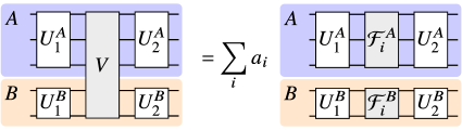
Consider a quantum circuit where the qubits are grouped into two partitions and , only connected by one possibly multi-qubit gate as shown in Fig. 1. Furthermore, assume the factorizing initial state and observable where the superscript labels the partition. These assumptions are, for example, satisfied when all qubits are initialized to and a Pauli string is measured. Circuit cutting, also referred to as circuit decomposition, circuit fragmentation or circuit knitting, is the task of finding a decomposition of the unitary channel corresponding to the gate so that
| (1) |
where are local channels on the partitions and as shown in Fig. 1 and are real expansion coefficients. For corresponding to and corresponding to , this decomposition allows us to determine the expectation value of the observable as
| (2) | ||||
| (3) | ||||
| (4) |
In Eq. 4 we denote by the expectation value with respect to the state on partition and , evolved by and , respectively, that is
| (5) |
for . If are unitary channels or measurement operations themselves, each term in the sum in Eq. 4 can be evaluated on a quantum computer. In the case of a more general quantum circuit, when all gates connecting the two partitions are cut, they become independent and the quantum circuits can be evaluated sequentially on a smaller device. We emphasize that the term circuit cutting as used here deals with decompositions of quantum circuits at the level of superoperators, rather than at the level of unitaries as in Ref. [32]. The output of a single experimental shot on a quantum computer is typically a bitstring. The expectation value of an observable is then obtained by a classical post-processing function on the bitstrings of multiple runs. Modeling the outcome of each experimental run as i.i.d. random variables, the number of required samples to achieve a given additive error is determined via the variance of the post-processing function. When a circuit is cut, the variance of the modified estimator for via Eq. 4 increases. Consequently, more experimental runs are required to estimate the result of the original circuit to the same given additive error. More specifically, this sampling overhead is exponential (in the number of cuts). The parameter
| (6) |
then quantifies the sampling overhead [25]. For completeness, this scaling behavior is re-derived in Appendix E. Eq. 1 is therefore optimal if the are chosen such that the 1-norm of the vector containing the coefficients is minimal. For cuts the sampling overhead is , however, joint cutting of multiple gates or wires leads to much smaller bounds for some gate types [26, 28]. Tab. 1 summarizes recent findings for cutting of CZ gates and wire cutting and compares the sampling complexities to the main results of the present work. In this work we cut multi-qubit controlled Z gates and provide upper bounds for . As we will explore in the next section, ZX calculus is particularly suited for this task.
3 ZX-calculus for circuit cutting
ZX calculus [33, 34] is a tensor-network representation for quantum circuits that together with powerful transformation rules allows diagrammatic reasoning. Since ZX-calculus has been reviewed elsewhere [35], we will only introduce those diagram types and transformation rules necessary for this article. The basic diagrams are Z-spiders, defined as
| (7) | ||||
| and X-spiders | ||||
| (8) | ||||
| where . For , the inset is commonly disregarded. A third tensor, a so-called H-box, is defined as | ||||
| (9) | ||||
where the sum runs over all . Spiders and H-boxes are therefore maps from - to (un-normalized) -qubit states, signified by the number of wires ending at the right and the left of the diagrams. When representing ZX diagrams as matrices, we will implicitly assume the computational basis. Then, for example, an H-box is a matrix filled with ones but a minus one in the lower right corner. H-boxes can be viewed as generalized Hadamard gates since
| (10) |
As apparent from the definitions, spiders and H-boxes correspond to symmetric tensors in all indices. Any quantum circuit can be represented as a ZX diagram, the reverse statement, however, is incorrect since a ZX diagram not necessarily corresponds to a unitary matrix. To obtain the Hermitian conjugate of a ZX diagram, we move all wires ending at the left to the right and those ending at the right to the left and replace all angles with their negative values. In the following we show how to use ZX calculus to decompose the unitary channel corresponding to an MCZ gate into a sum over unitary and measurement channels. Decomposing circuits into simpler parts using ZX calculus has been done before in Refs. [36, 37].
An MCZ gate enjoys a simple representation [38]
| (11) |
in terms of an H-box with zero wires on the left as shown in Appendix A. In matrix representation, and we will refer to the number of qubits involved in the MCZ gate as the order of the gate. Also note that there is no difference between the control and target qubits in an MCZ gate. The decomposition constructed in this article is based on the H-box fusion rule [38]
| (12) |
proved in Appendix B for completeness.
Consequently, with Eq. 12 applied to Eq. 11, the unitary channel action corresponding to the MCZ gate of order acting on an arbitrary density matrix , takes the form
| (13) |
The two partitions (upper qubits, lower qubits) are only connected by the tensor shaded in grey, the un-normalized Choi operator of a Hadamard gate. Next, we remove the two remaining connections between the partitions by a rank-one decomposition of in terms of vectors factorizing over the two partitions
| (14) | ||||
| (15) |
In Eq. 15 we introduced the diagrammatic notation for a two-dimensional vector
| (16) |
where is the -th component of . Therefore, the H-box fusion rule in Eq. 13 reduces the cutting of an MCZ gate to the decomposition of a four-by-four matrix. However, only vectors and are useful whose contraction with the H-box results in channels that can be evaluated on a quantum computer. In Appendix C we prove the identities
![[Uncaptioned image]](/html/2302.00387/assets/x22.png)
|
(17) | |||
| for and | ||||
![[Uncaptioned image]](/html/2302.00387/assets/x25.png)
|
(18) | |||
where denotes the projector on . The identities Eq. 17 and Eq. 18 suggest for different values of . This choice guarantees a decomposition consisting of unitary controlled Z-rotation gates and projectors, which can be evaluated by mid-circuit measurements. Next, we expand in the basis spanned by the Pauli matrices and then substitute their spectral representation
| (19) | |||
| (20) | |||
| (21) |
and additionally the identity matrix in terms of the eigenvectors of the Pauli matrix, that is
. The choice of this expansion basis leads to for the normalized version of which can be shown to be optimal with the help of the robustness of entanglement measure [26, 27].
Unfortunately, Eq. 19 contains the state
![[Uncaptioned image]](/html/2302.00387/assets/x30.png) , not covered by Eq. 17 and Eq. 18 and its contraction with an H-box does not result in a valid quantum circuit.
We could simulate this operation by an MCZ gate on an ancilla qubit initialized in and postselected on the state [39], however, at the cost of one ancilla qubit per partition and cut.
We circumvent this issue by substituting instead.
By this substitution we lose optimality for the decomposition of . But note that it is unknown if an optimal decomposition of translates into an optimal decomposition of the MCZ gate. While we show only upper bounds, we observe in Sec. 4 the reduction of the general decomposition of an MCZ gate for a CZ gate to the optimal one. With these considerations in mind and defining , we find
, not covered by Eq. 17 and Eq. 18 and its contraction with an H-box does not result in a valid quantum circuit.
We could simulate this operation by an MCZ gate on an ancilla qubit initialized in and postselected on the state [39], however, at the cost of one ancilla qubit per partition and cut.
We circumvent this issue by substituting instead.
By this substitution we lose optimality for the decomposition of . But note that it is unknown if an optimal decomposition of translates into an optimal decomposition of the MCZ gate. While we show only upper bounds, we observe in Sec. 4 the reduction of the general decomposition of an MCZ gate for a CZ gate to the optimal one. With these considerations in mind and defining , we find
| (22) | ||||
| (23) |
where for and otherwise. This result leads to a general decomposition of the MCZ gate by substituting Eq. 23 into Eq. 13 and then contracting the vectors with the H-boxes with the help of Eq. 17 and Eq. 18. Before we state the resulting decomposition explicitly, we rewrite the superoperator corresponding to the projector in Appendix D with the result
| (24) |
Here, the operation abbreviates the sum over the unitary channels corresponding to all combinations of one-qubit identities and Z gates, that is for an -qubit state
| (25) |
The second operation is where are the projectors on all elements of the computational basis and for as well as otherwise. We show in Appendix E how to relate to circuits with intermediate measurements. Furthermore, we prove that circuits containing either or have the same sampling complexity, but introducing leads to gate cancellations in the final decomposition. The consequence is a reduction of in the final result.
We now state the main result of this article, the decomposition of an MCZ gate:
| (26) |
Here, denotes an S gate and
| (27) |
symbolizes the operation in circuit form. The decomposition shown here is for an MCZ gate of order five and a cut after the third qubit line counting from the top. We emphasize that since the derivation was independent of the order of the MCZ gate and the cutting location, the structure of the decomposition in Eq. 26 remains unchanged for a cut at any position and arbitrary order of the MCZ gate. Eq. 26 has to be read in terms of channels. To evaluate a quantum circuit containing an MCZ gate we have to subsequently replace the gate by the gates and operations shown in Eq. 26.
4 Sampling overhead
In this section we investigate the sampling overhead associated with Eq. 26 for different orders of the MCZ gate. The sampling overhead is characterized by as stated in Eq. 6. We re-derive this statement in detail in Appendix E. We also consider operations such as and show that with regard to sampling overhead, this operation can be treated in the same manner as a unitary channel. With this insight, we are now in the position to determine for Eq. 26. Recalling the pre-factor for the unitary circuits summarized by in Eq. 27, we find for a general MCZ gate . Remarkably, this bound holds independently of the order of the gate. In the right bracket of Eq. 26 the MCZj gate is the identity gate for and also contains the identity gate but the prefactors have a different sign. Consequently, summing these gates slightly reduces . This reduction becomes more pronounced, the smaller the order of the MCZ gate is but quickly approaches for large order. Indeed, for a CZ gate, the right bracket vanishes and we find which is known to be optimal [26]. Similarly, a cut separating one qubit line from a general MCZ gate results in . For a CCZ gate, we find . Due to the importance of CCZ gates in quantum computing theory, its decomposition is stated explicitly:
| (28) |
with the abbreviation
| (29) |
The sampling complexities derived above are summarized in Tab. 2 together with known results on the optimality of the decomposition.
| gate type | optimality | |
|---|---|---|
| CZ gate | 3 | optimal [26] |
| CCZ gate | 4.5 | unknown |
| one qubit removed | 5 | unknown |
| general | 6 | unknown |
5 Experiments on IBM Q
In this section, we show experimental results obtained on the ibmq_ehningen system. We will find a strong reduction of noise impact for the proposed cutting scheme.
We first run numerical simulations to validate the proposed MCZ cutting scheme. To this end, we generate a set of random 3, 4 and 5 qubit circuits with one MCZ gate at the center of the circuit and two otherwise independent partitions. For exemplary circuits and a more detailed description of the circuit generation, see Supplemental Material. In all experiments, we measure the Pauli string. For the cut circuits, we allocate samples to each circuit pair labeled by where bounds the standard deviation by , see Eq. 68 in Subsec. E.2. For an uncut circuit, we allocate all samples for evaluation. We first calculate and via Eq. 68, the number of repetitions required to bound the standard deviation of expectation values of the cut circuit to within and . For fixed number of qubits we generate 5 random circuits and sample each circuit times using an ideal simulator. Repeating this process 20 times, generates one hundred data points for each value of .
We now compare the distributions of the expectation-value differences between the full (that is uncut) and cut circuits for different values of .
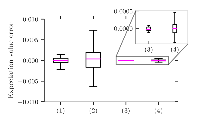
We run simulations for 3,4 and 5 qubits and find almost no difference in the standard deviations of the distributions. This behavior is expected since is independent from the order of the MCZ gate. Exemplarily, Fig. 2 shows the distribution for random 5-qubit circuits.
In the figure, the white boxes are the interquartile ranges and the bars denote the 5% and 95% quantiles. Fig. 2(1) shows the distribution of the expectation values for the original uncut circuits. As expected, the distribution becomes broader when we instead evaluate the cut circuit in Fig. 2(2). Its standard deviation is , which is smaller than the chosen value of . The same effect is observed for shown in the plots in Fig. 2(3) and Fig. 2(4). Consequently, a tighter version of Eq. 68 to bound the variance might exist.
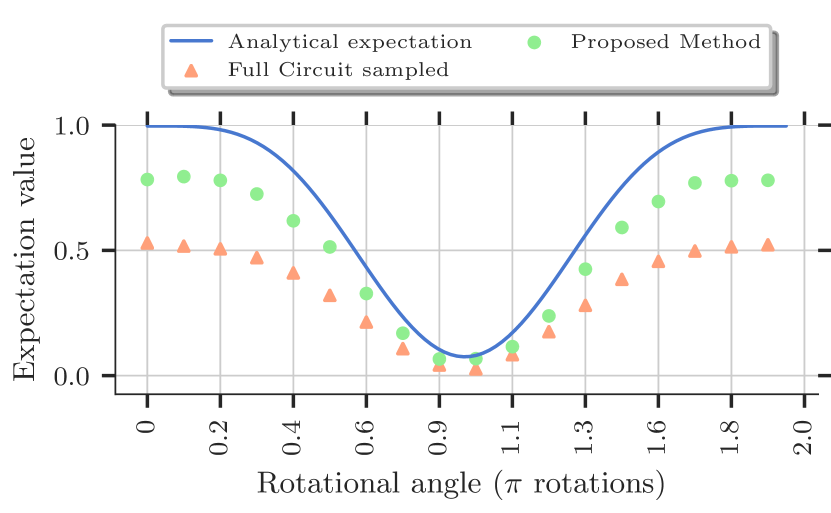
To further validate the proposed method on real quantum hardware and analyze the impact of noise, we performed MCZ gate-cutting experiments on the ibmq_ehningen [40] device. The ibmq_ehningen device is a super-conducting qubit type quantum hardware with a 27 qubit ibmq_falcon processor. The native gate set on this hardware consists of Rotational-Z, Pauli-X, , Identity, and CNOT gates. For the experiments, we again generated a random circuit with one free parameter that was scanned in the experiments.
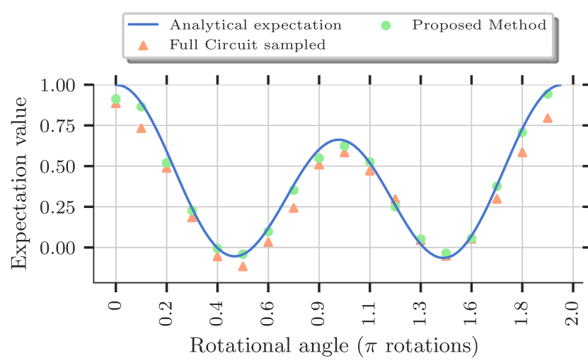
The maximum number of shots per job on the ibmq_ehningen device is and the same was used for each data point, see Supplemental Material for the explicit circuits and a more detailed discussion of the experimental setup. Fig. 4 shows the result for a three-qubit circuit containing a CCZ gate. In the figure, the results obtained by cutting the CCZ gate (green circles) lie slightly closer to the exact curve (blue line) than the results from the uncut circuit (orange triangles).
Next, we repeated the experiment with a five-qubit circuit containing an MCZ gate of order five. The result is shown in Fig. 5.
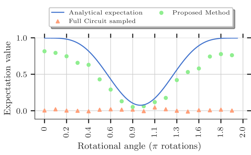
From the figure, it is clear that the influence of noise is extreme when executing the transpiled version of the full circuit with an MCZ gate of order five. The resulting expectation values were nothing but a random output centered around zero. However, the expectation value estimated using the proposed method falls much closer to the expectation values obtained by ideal simulation. This resilience to noise can be attributed to the strong reduction of the CNOT-gate count in the cut circuits. While, asymptotically, an MCZ gate of order can be synthesized with CNOT gates with one auxiliary qubit [41], for small the number of required CNOT gates increases quickly. Consequently, cutting for example two qubits from an MCZ gate of order five reduces the maximum number of CNOT gates in a circuit to those required to synthesize a double-controlled S gate. This reduction becomes even more pronounced after compiling to topologically restricted hardware. As a consequence, we observe a strong reduction of noise impact. The maximum number of CNOT gates present in the different circuits are shown in Tab. 3. The number of CNOT gates might vary based on the transpilation method used. However, we chose to proceed with the best transpiler offered by the hardware manufacturer to validate our results.
| gate type | CNOT | CNOT cut |
|---|---|---|
| CCZ gate | 13 | 3 |
| 5-qubit MCZ | 114 | 32 |
As most of the work in the literature is conducted via a simulator, we extended our 5-qubit MCZ experiment shown above to a noisy simulator. The results are shown in Fig. 3. The proposed method still outperforms the full circuit execution even though the noise model provided by the manufacturer does not accurately capture the noise level exhibited by the real device.
6 Conclusion
In this work, we proposed an approach for cutting multi-controlled Z gates by means of ZX-calculus based on the H-box fusion rule. We derived the upper bound on the sampling overhead that is independent of the order of the gate. We validated the results on IBM hardware and found strong noise reduction due to the reduced amount of CNOT gates in the cut circuit. We anticipate the generalization of our method to multi-controlled rotation gates and extension to multi-qubit rotations. The optimality of the decompositions constructed in this work at present remains an open question.
Acknowledgements
We thank L. Burgholzer and R. Wille for fruitful exchange and discussion.
We acknowledge the use of IBM Quantum services for this work. The views expressed are those of the authors, and do not reflect the official policy or position of IBM or the IBM Quantum team.
The research was supported by the Bavarian Ministry of Economic Affairs, Regional Development and Energy with funds from the Hightech Agenda Bayern and by the Bavarian Ministry for Economic Affairs, Infrastructure, Transport and Technology through the Center for Analytics-Data-Applications (ADA Center) within the framework of “BAYERN DIGITAL II”.
The research was furthermore funded by the project QuaST, supported by the Federal Ministry for Economic Affairs and Climate Action on the basis of a decision by the German Bundestag.
Appendix A Representation of an MCZ gate
In this appendix, we prove the representation of an MCZ gate as stated in Eq. 11. We begin by introducing the diagrammatic notation of a general -qubit column vector as
| (30) |
With this definition and the -spider
| (31) |
see Eq. 7, we obtain
![[Uncaptioned image]](/html/2302.00387/assets/x69.png)
|
(32) | |||
| (33) |
To guarantee that the correct indices are contracted, we inserted one-qubit identities . Consequently, Eq. 33 is proportional to a unitary matrix if all elements of have the same absolute value or to a projector on a computational basis state if all but one element of are zero. We are now in the position to prove Eq. 11 by setting
| (34) |
where we recalled the definition of an H-box from Eq. 9. Consequently, from Eq. 33, we find for Eq. 11, the matrix representation of an MCZ gate.
Appendix B Proof of H-box fusion rule
We proof Eq. 12 from the right to the left. We first define the joint indices and as well as and . We then find in Dirac notation with the indices and running over , and
| (35) | |||
| (36) | |||
| (37) |
which is equivalent to the left-hand side of Eq. 12. In the last step we recalled that so that
| (38) | |||
| (39) | |||
| (40) |
Alternatively, the H-box-fusion rule can be derived by the Schmidt decomposition of the vector representing the diagonal elements of the unitary corresponding to the MCZ gate.
Appendix C H-box identities
In this appendix, we prove Eq. 17 and Eq. 18. The contraction of a single-qubit vector with an H-box is readily calculated as
![[Uncaptioned image]](/html/2302.00387/assets/x72.png)
|
(41) | |||
| by matrix-vector multiplication. Consequently, making use of Eq. 33, we find | ||||
![[Uncaptioned image]](/html/2302.00387/assets/x73.png)
|
(42) | |||
Therefore, Eq. 42 is proportional to a unitary for and to a projector on the state for . In terms of spiders, these two conditions are either satisfied for or for . The former results in Eq. 17 and the latter in Eq. 18.
Appendix D Rewriting the Projector
To prove Eq. 24, we first restate the definition of from Eq. 25
| (43) |
for an -qubit state . For a single-qubit state we note that
| (44) |
by substituting as well as into the left-hand side of Eq. 44. Consequently, by applying Eq. 44 iteratively, Eq. 43 becomes
| (45) |
Finally, we rewrite Eq. 45 as
| (46) | ||||
| (47) | ||||
| (48) |
where for and otherwise, which proves Eq. 24.
Appendix E Derivation of sample-complexity overhead
This appendix investigates in more detail the sampling overhead associated with evaluating a cut circuit, closely following Refs. [24, 7]. In Subsec. E.1 we prove the statements on sampling overhead made in the main text for the case where in each experimental run a circuit from the decomposition is sampled from a probability distribution. Subsequently, in Subsec. E.2 we bound the variance by pre-estimating the expectation values of the partitioned circuits.
E.1 Sample complexity for circuit sampling
Consider an -qubit quantum circuit. Assume the initial state and consider the post-processing function on the measured bitstring . Furthermore, assume that can be efficiently calculated classically. These definitions describe the computational model of Refs. [42, 7]. The post-processing function gives rise to an observable via
| (49) |
where is the projector on the computational basis state corresponding to bitstring . Conversely, for instance, if the observable is a Pauli string, it can be written in the above form by local diagonalization and viewing the unitary diagonalization matrix as part of the circuit. The goal of the quantum computation is to approximate to additive error with high probability for which we will define statistical estimators in the following.
Cutting a gate amounts to replacing its superoperator by a decomposition as in Eq. 1. We first consider the case where all in the decomposition correspond to unitary gates. With this substitution, we find
| (50) |
where denotes the expectation value with respect to the state evolved by circuit , containing . Moreover, is the probability to measure bitstring given circuit . To evaluate the result on a quantum device, we sample at each experimental run according to the probability distribution
| (51) |
We therefore define a random variable that takes values with probability and the estimator [25]
| (52) |
where the random variable models the bitstring outcomes of the circuit . This estimator is unbiased since
| (53) | ||||
| (54) | ||||
| (55) | ||||
| (56) |
Here, we substituted Eq. 51 into Eq. 54. The final result is obtained by comparing Eq. 55 to Eq. 50. The estimator for shots is given by the sample mean of Eq. 52. Thus, to estimate to additive error with probability , Hoeffding’s inequality provides the required number of experimental repetitions as
| (57) |
where we used that . The number of samples needed for the original circuit is obtained for in Eq. 57 from which we infer the sampling overhead .
It is straightforward to generalize this derivation to cuts. In this case, the expectation value of the observable is obtained as
| (58) |
and the estimator for cuts becomes
| (59) |
where we defined the independent random variables ,…, that determine the specific circuit to run. To show equality between the expectation value of Eq. 59 and Eq. 58, we follow Eq. 53 to Eq. 56 and make use of the independence of ,…,. Since , Hoeffding’s inequality applied to the sample mean of Eq. 59, provides the bound on the sampling overhead. If the observable factorizes over the partitions and of the original circuit, the post-processing function factorizes as well, that is where and are the bitstring results on partition and . If the initial state factorizes and all gates connecting the two partitions are cut, the partitioned circuits can be evaluated on independent quantum computers or sequentially on the same device.
We now turn to a quantum circuit that contains projectors. Consider the map consisting of a complete set of projectors and with
| (60) |
for state . This map is neither positive since can be smaller than zero, nor trace preserving since the state in Eq. 60 is not normalized after the projection and multiplied by . Note that both and of Eq. 24 are instances of . For we set only for and zero otherwise. On the other hand for we have for and otherwise. Even though does not correspond to a physical time evolution, we can nevertheless estimate
| (61) |
by repeated use of a quantum computer. In Eq. 61, the density matrix is the state right before the projectors and is the unitary channel corresponding to the unitary evolution afterwards until the final measurement. To estimate on a quantum computer, we perform intermediate measurements, and sample according to the estimator
| (62) |
where the random variable describes the bitstring outputs of the final measurements as before and the random variable models the outcomes of the intermediate measurements. According to Eq. 62 we have to add in the sample mean for if we found the all-one state in the intermediate measurement and otherwise. This estimator is unbiased since
| (63) | ||||
| (64) | ||||
| (65) | ||||
| (66) |
The first line, Eq. 63, is the definition of the expectation value and in Eq. 64 we substituted [1]. In the final step, we identified . The number of samples required to determine to given additive error is again determined by Hoeffding’s inequality applied to the sample mean of Eq. 62. Since by definition, Eq. 57 remains unchanged when some of the circuits contain projectors.
E.2 Sampling complexity by pre-estimating circuits
In Sec. 5, we show experimental results for a circuit that disintegrates into two independent partitions and . After cutting the single gate that connects the two partitions, we have to evaluate
| (67) |
Rather than sampling a circuit pair for each experimental run as discussed in Subsec. E.1 we pre-estimate the expectation values and for all the circuits first and subsequently restore the result of the original circuit with the help of Eq. 67. In the following, it is shown that the standard deviation of Eq. 67 can be bounded by for a total number of experimental runs
| (68) |
where we allocate
| (69) |
samples to each circuit of circuit pair to determine the expectation values and . Note that . Next, we define the estimator
| (70) |
where and . Since and are independent, this estimator is unbiased. The variance of is calculated as
| (71) | ||||
| (72) | ||||
| (73) | ||||
| (74) |
In Eq. 71 we first factorized the variance, valid for independent random variables. Eq. 73 makes use of the bounds and since and . Finally, for independent samples. Consequently,
| (75) | ||||
| (76) | ||||
| (77) |
References
- [1] M. A. Nielsen and I. L. Chuang. “Quantum computation and quantum information: 10th anniversary edition”. Cambridge University Press. (2010).
- [2] J. Preskill. “Quantum Computing in the NISQ era and beyond”. Quantum 2, 79 (2018).
- [3] P.W. Shor. “Algorithms for quantum computation: discrete logarithms and factoring”. In Proceedings 35th Annual Symposium on Foundations of Computer Science. Page 124. IEEE Comput. Soc. Press (1994).
- [4] L. K. Grover. “A fast quantum mechanical algorithm for database search”. In Proceedings of the Twenty-Eighth Annual ACM Symposium on Theory of Computing. Page 212. New York, NY, USA (1996). Association for Computing Machinery.
- [5] E. Farhi, J. Goldstone, and S. Gutmann. “A quantum approximate optimization algorithm” (2014). arXiv:1411.4028.
- [6] “IBM Development Roadmap 2022”. https://www.ibm.com/quantum/roadmap. Accessed: 2023-01-02.
- [7] T. Peng, A. W. Harrow, M. Ozols, and X. Wu. “Simulating large quantum circuits on a small quantum computer”. Phys. Rev. Lett. 125, 150504 (2020).
- [8] M. A. Perlin, Z. H. Saleem, M. Suchara, and J. C. Osborn. “Quantum circuit cutting with maximum-likelihood tomography”. NPJ Quantum Inf. 7, 64 (2021).
- [9] G. Uchehara, T. M. Aamodt, and O. Di Matteo. “Rotation-inspired circuit cut optimization”. In 2022 IEEE/ACM Third International Workshop on Quantum Computing Software (QCS). Page 50. Los Alamitos, CA, USA (2022). IEEE Computer Society.
- [10] D. Chen, B. Baheri, V. Chaudhary, Q. Guan, N. Xie, and S. Xu. “Approximate quantum circuit reconstruction”. In 2022 IEEE International Conference on Quantum Computing and Engineering (QCE). Page 509. (2022).
- [11] C. Ying, B. Cheng, Y. Zhao, H.-L. Huang, Y.-N. Zhang, M. Gong, Y. Wu, S. Wang, F. Liang, J. Lin, Y. Xu, H. Deng, H. Rong, C.-Z. Peng, M.-H. Yung, X. Zhu, and J.-W. Pan. “Experimental simulation of larger quantum circuits with fewer superconducting qubits”. Phys. Rev. Lett. 130, 110601 (2023).
- [12] T. Ayral, F.-M. Le Régent, Z. Saleem, Y. Alexeev, and M. Suchara. “Quantum divide and compute: Hardware demonstrations and noisy simulations”. In 2020 IEEE Computer Society Annual Symposium on VLSI (ISVLSI). Page 138. (2020).
- [13] T. Ayral, F.-M. Le Régent, Z. Saleem, Y. Alexeev, and M. Suchara. “Quantum divide and compute: Exploring the effect of different noise sources”. SN comput. sci. 2, 132 (2021).
- [14] J. Liu, A. Gonzales, and Z. H. Saleem. “Classical simulators as quantum error mitigators via circuit cutting” (2022). arXiv:2212.07335.
- [15] R. Majumdar and C. J. Wood. “Error mitigated quantum circuit cutting” (2022). arXiv:2211.13431.
- [16] W. Tang, T. Tomesh, M. Suchara, J. Larson, and M. Martonosi. “CutQC: Using small quantum computers for large quantum circuit evaluations”. In Proceedings of the 26th ACM International Conference on Architectural Support for Programming Languages and Operating Systems. Page 473. ASPLOS 2021New York, NY, USA (2021). Association for Computing Machinery.
- [17] W. Tang and M. Martonosi. “ScaleQC: A scalable framework for hybrid computation on quantum and classical processors” (2022). arXiv:2207.00933.
- [18] T. Chatterjee, A. Das, S. I. Mohtashim, A. Saha, and A. Chakrabarti. “Qurzon: A prototype for a divide and conquer-based quantum compiler for distributed quantum systems”. SN Computer Science 3, 323 (2022).
- [19] K. Mitarai and K. Fujii. “Methodology for replacing indirect measurements with direct measurements”. Phys. Rev. Research 1, 013006 (2019).
- [20] K. Mitarai and K. Fujii. “Constructing a virtual two-qubit gate by sampling single-qubit operations”. New J. Phys. 23, 023021 (2021).
- [21] K. Mitarai and K. Fujii. “Overhead for simulating a non-local channel with local channels by quasiprobability sampling”. Quantum 5, 388 (2021).
- [22] K. Temme, S. Bravyi, and J. M. Gambetta. “Error mitigation for short-depth quantum circuits”. Phys. Rev. Lett. 119, 180509 (2017).
- [23] C. Piveteau, D. Sutter, and S. Woerner. “Quasiprobability decompositions with reduced sampling overhead”. NPJ Quantum Inf. 8, 12 (2022).
- [24] C. Piveteau. “Advanced methods for quasiprobabilistic quantum error mitigation”. Master’s thesis. ETH Zurich. (2021). url: https://www.research-collection.ethz.ch/handle/20.500.11850/504508.
- [25] H. Pashayan, J. J. Wallman, and S. D. Bartlett. “Estimating outcome probabilities of quantum circuits using quasiprobabilities”. Phys. Rev. Lett. 115, 070501 (2015).
- [26] C. Piveteau and D. Sutter. “Circuit knitting with classical communication” (2022). arXiv:2205.00016.
- [27] G. Vidal and R. Tarrach. “Robustness of entanglement”. Phys. Rev. A 59, 141 (1999).
- [28] A. Lowe, M. Medvidović, A. Hayes, L. J. O’Riordan, T. R. Bromley, J. M. Arrazola, and N. Killoran. “Fast quantum circuit cutting with randomized measurements”. Quantum 7, 934 (2023).
- [29] Z. H. Saleem, T. Tomesh, M. A. Perlin, P. Gokhale, and M. Suchara. “Divide and conquer for combinatorial optimization and distributed computing” (2021). arXiv:2107.07532.
- [30] S. Hadfield. “Quantum algorithms for scientific computing and approximate optimization” (2018). arXiv:1805.03265.
- [31] T. Yamamoto and R. Ohira. “Error suppression by a virtual two-qubit gate”. J. Appl. Phys. 133, 174401 (2023).
- [32] S. C. Marshall, C. Gyurik, and V. Dunjko. “High Dimensional Quantum Machine Learning With Small Quantum Computers”. Quantum 7, 1078 (2023).
- [33] B. Coecke and R. Duncan. “Interacting quantum observables: categorical algebra and diagrammatics”. New J. Phys. 13, 043016 (2011).
- [34] B. Coecke and R. Duncan. “Interacting quantum observables”. In L. Aceto, I. Damgård, L. A. Goldberg, M. M. Halldórsson, A. Ingólfsdóttir, and I. Walukiewicz, editors, Automata, Languages and Programming. Page 298. Berlin, Heidelberg (2008). Springer Berlin Heidelberg.
- [35] J. van de Wetering. “ZX-calculus for the working quantum computer scientist” (2020). arXiv:2012.13966.
- [36] A. Kissinger and J. van de Wetering. “Simulating quantum circuits with zx-calculus reduced stabiliser decompositions”. Quantum Sci. Technol. 7, 044001 (2022).
- [37] A. Kissinger, J. van de Wetering, and R. Vilmart. “Classical simulation of quantum circuits with partial and graphical stabiliser decompositions”. In F.s Le Gall and T. Morimae, editors, 17th Conference on the Theory of Quantum Computation, Communication and Cryptography (TQC 2022). Volume 232 of Leibniz International Proceedings in Informatics (LIPIcs), page 5:1. Dagstuhl, Germany (2022).
- [38] M. Backens and A. Kissinger. “ZH: A complete graphical calculus for quantum computations involving classical non-linearity”. Electron. Proc. Theor. Comput. Sci. 287, 23 (2019).
- [39] “van de Wetering, J.”. Private communication.
- [40] “IBM Quantum”. https://quantum-computing.ibm.com/. Accessed: 2023-01-23.
- [41] A. Barenco, C. H. Bennett, R. Cleve, D. P. DiVincenzo, N. Margolus, P. Shor, T. Sleator, J. A. Smolin, and H. Weinfurter. “Elementary gates for quantum computation”. Phys. Rev. A 52, 3457 (1995).
- [42] S. Bravyi, G. Smith, and J. A. Smolin. “Trading classical and quantum computational resources”. Phys. Rev. X 6, 021043 (2016).
- [43] “Github repository MCZ-gate cutting”. https://github.com/ChristianUfrecht/MCZgate_cutting.
- [44] E. van den Berg, Z. K. Minev, and K. Temme. “Model-free readout-error mitigation for quantum expectation values”. Phys. Rev. A 105, 032620 (2022).
Supplementary material
In this supplemental material, we provide more details on our simulations and experiments on the ibmq_ehningen system.
Random circuits
For our numerical simulations in Sec. V of the main article we generated a set of random circuits consisting of about on average 30 single-qubit , and rotations and 10 CNOT gates. We generated circuits with 3, 4, or 5 qubits with one MCZ gate in the center, accordingly, of order 3, 4, or 5. Two instances of these circuits are shown in Fig. 6 and Fig. 7. In the 3-qubit circuits, one 1-qubit and one 2-qubit partition, and in the 5-qubit circuits one 2-qubit and one 3-qubit partition are only connected by the MCZ gate. For the numerical evaluation, we choose the Pauli string as observable. For generating the random circuits, we impose the constraint that the MCZ gate in the circuits should have a significant impact on the expectation value of the observable in order to be able to resolve its influence on the result with the available number of experimental runs. That is, the difference in the expectation value between a circuit with and without MCZ is chosen to be greater than 0.2. A proof-of-concept implementation of MCZ-gate cutting for arbitrary order of the gate is available on GitHub [43].

Experiments on ibmq_ehningen
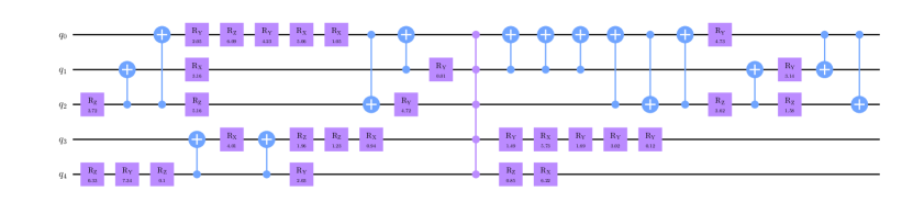
In this part of the supplemental material, we provide more details on the experimental setup. For the experiments we (1) again generated a random 3-qubit circuit and a 5-qubit circuit with two partitions, only connected by a CCZ gate and an MCZ gate of order 5, respectively. The circuits are shown in Fig. 8 and Fig. 9. Subsequently, we optimized the single-qubit rotation angles until the difference of the expectation values of a Pauli Z-string with respect to the circuit with and without the MCZ gate was maximal. Finally, we added one free parameter to the rotation angles of three single-qubit rotation gates, which were scanned in the experiments. The parameter is denoted by psi in the circuits shown in Fig. 8 and Fig. 9. (2) We used the highest level of optimization offered by the Qiskit API after transpiling the circuits to the native gate set and the hardware graph of the ibmq_ehningen device. The highest level of optimization first searches for a layout that satisfies all the 2-qubit gate connectivity to the hardware graph considering the qubits readout errors and gate fidelities. Then the circuit is unrolled to the native gate set. Finally, optimizations in the form of commutative gate cancellation and re-synthesis of two-qubit unitary blocks are performed. (3) 18 data points between with equal intervals were chosen for scanning the free parameter. (4) We used shots per data point, the maximum number of shots per job allowed by the ibmq_ehningen device. (5) All experiments were run with maximum error mitigation offered by ibmq wherever possible. We used the TREX option for readout-error mitigation [44] offered by Qiskit. (6) The ibmq_ehningen device can be characterized by the following parameters [40]: It is a 27 qubit ibmq_falcon processor, whose connectivity graph is shown in Fig. 10. The noise parameters at the time of our experiments were the following: Decoherence times: Average values µs and µs with large fluctuations between the qubits. Single-qubit errors are of the order of and CNOT-gate errors of the order of .