Self-supervised learning for gravitational wave signal identification

Abstract

The computational cost of searching for gravitational wave (GW) signals in low latency has always been a matter of concern. We present a self-supervised learning model applicable to the GW detection. Based on simulated massive black hole binary signals in synthetic Gaussian noise representative of space-based GW detectors Taiji and LISA sensitivity, and regarding their corresponding datasets as a GW twins in the contrastive learning method, we show that the self-supervised learning may be a highly computationally efficient method for GW signal identification.

I Introduction

The field of gravitational wave (GW) detection has seen an explosion of compact binary coalescence signals over the past several years LIGOScientific:2016aoc ; LIGOScientific:2016sjg ; LIGOScientific:2017bnn ; LIGOScientific:2017vwq ; LIGOScientific:2018mvr ; LIGOScientific:2020ibl .

Recently, 93 GW events have been reported LIGOScientific:2021djp . It is expected that over the coming years, more GW events, including binary black holes (BBH), binary neutron stars (BNS), as well as other exotic sources will be observed more frequently. As such, the need for more efficient search methods will be more important as the detectors improve in sensitivity.

It is well-known that identifying signal is achieved, in part, using a technique known as template-based matched filtering, which uses a bank Brown:2012qf ; DalCanton:2017ala ; Harry:2009ea ; DalCanton:2014hxh ; Ajith:2012mn of template waveforms Sathyaprakash:1991mt ; Taracchini:2013rva ; Privitera:2013xza ; Blanchet:2013haa spanning a large astrophysical parameter space. The corresponding waveform models that cover the inspiral, merger, and ringdown phases of a compact binary coalescence are based on combining post-Newtonian theory Arun:2008kb ; Buonanno:2009zt ; Mishra:2016whh , the effective-one-body method Buonanno:1998gg , and numerical relativity simulations Pretorius:2005gq . However, the algorithms used by the search pipelines to make detections are computationally expensive, since the large parameter space, as well as analysis of the high frequency components of the waveform, inevitably result in large computational cost.

Recently, the deep learning has been in popularity Goodfellow:2014upx ; Simonyan:2014cmh ; Yuille:2014lcc ; Fergus:2013mdz ; Szegedy:2014nrf , which is a subset of machine learning. The advantage of deep learning is that the computationally intensive stage is pre-computed, so it is able to performing analyses rapidly. Its successful implementations include image processing Efros:2016aae ; Karpathy:2014lff , medical diagnosis, in particular GW field, such as glitch classification Mukund:2016thr ; Zevin:2016qwy ; George:2017fbn and signal identification George:2016hay ; Wei:2019zlc ; Xia:2020vem ; Lin:2020aps ; Liao:2021vec ; Ruan:2021fxq ; Bacon:2022lsm ; Zhao:2022qob ; Schafer:2022dxv ; Murali:2022sba ; Nousi:2022dwh ; Shen:2019vep ; Ren:2022hny .

However, the deep learning method currently used for searching for the GW signals is often limited to building supervised learning models, which are indeed trained on scarcely labelled or simulated data and thus suffer from biases or small training sizes when applied to new or full datasets. Thus it is significant to consider the tailored deep learning models in a self-supervised, semi-supervised or unsupervised manner Hinton:2002knh ; Maaten:1912mlm .

In this paper, we report the construction of a self-supervised learning that can reproduce the searching for massive black hole binary (MBHB) GW signals. A contrastive learning method, the GW twins, which applies redundancy-reduction to self-supervised learning Deny:2103:mld , is proposed. Based on simulated MBHB signals in synthetic Gaussian noise representative of space-based GW detectors Taiji Hu:2017mde and LISA LISA:2017pwj sensitivity, we investigate whether the self-supervised learning can efficiently identify a signal present in the data, or the data contain only detector noise.

II Method

II.1 Description of GW twins

In self-supervised learning for GW detection, our GW twins operates on a joint embedding of augmentation vectors, see Fig.1. In detail, it produces two augmentation vectors for all data of a batch $h$ sampled from a dataset. In our case, we consider the batch of $h$ as an injected GW waveform signal. The augmentation vectors are obtained with a distribution of data augmentations $\mathcal{T}$ (the light blue area in Fig.1). Two batches of augmentation vectors $d^{A}$ and $d^{B}$ are fed to a deep network $f_{\theta}$ (covered by the light yellow area in Fig.1), producing batches of embeddings $h^{A}$ and $h^{B}$, respectively.

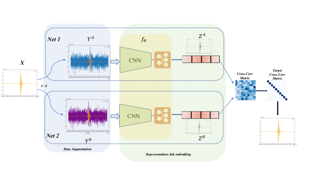
Figure 1: The objective function of GW twins measures the cross-correlation matrix between the embeddings of two identical networks $h^{A}$ and $h^{B}$ (described as the extraction of GW signal by Net A and Net B) fed with augmentation versions of a batch of samples $d^{A}$ and $d^{B}$ (covered by the light blue area). Here, $d^{A}=h+n_{L}$ and $d^{B}=h+n_{T}$, and the cross-correlation matrix is made close to the identity. This causes the embedding vectors of distorted versions of a sample (blue and purple signal waveforms) to be similar, while minimizing the redundancy between the components of the embedding vectors.

In our GW twins design, the corresponding loss function $\mathcal{L}_{GW}$ is

$$\mathcal{L}_{GW}=\underbrace{\sum_{i}\left(1-C^{GW}_{ii}\right)^{2}}_{\text{invariant part}}+~{}~{}\lambda\underbrace{\sum_{i}\sum_{j\neq i}\left({C^{GW}_{ij}}\right)^{2},}_{\text{redundancy reduction part}}$$ (1)

where

$$C^{GW}_{ij}=\frac{\sum_{b}h^{A}_{b,i}h^{B}_{b,j}}{\sqrt{\sum_{b}{(h^{A}_{b,i})}^{2}}\sqrt{\sum_{b}{(h^{B}_{b,j})}^{2}}}$$ (2)

is the cross-correlation matrix computed between the outputs of two identical networks, with the values comprised between -1 (i.e. perfect anti-correlation) and 1 (i.e. perfect correlation), $\lambda$ is a positive constant, $b$ is batch samples, and $i,j$ represent the vector dimension of the networks outputs

Here, the objective function (OF) is understood as an instantiation of the information bottleneck (IB) objective Tishby:2000:tpb ; Tishby:1503:tzy . It is easy to see that our OF has similarities with existing OFs for self-supervised learning, for example, the redundancy reduction part plays a role similar to the contrastive part in the infoNCE objective Vinyals:1807:olv .

II.2 Implementation Details

It is often hard to find a large collection of correctly labelled data. This scarcity of labelled real data exists for GW events as well. One way to combat this shortage is to train on simulated data and hope the trained model is useful for the real dataset as well. The success of such an approach is dependent on the quality of simulation. However, we will have rich raw data in GW detection, specially for space-based detectors, such as Taiji and LISA. Thus the application of self-supervised training can be particularly relevant for GW signal detection.

The basic idea of our GW twins design for self-supervised training is to have two dataset which see different versions of GW data and use the OF of GW twins to learn embeddings. In details, we can feed the data $d^{A}$ from LISA into Net A and the data $d^{B}$ from Taiji into Net B. In Fig.1, the blue strain and purple strain in the data augmentation waveform plottings which are covered by the light blue area correspond to the LISA noise data strain $n_{L}$ and the Taiji noise data strain $n_{T}$, the orange waveform is the GW signal $h$. Since the noise in Taiji is different from LISA, we can imagine it as an augmented sample of the same underlying signal.

It is well-known that most self-supervised works focused on images, and so usually inputs are images and 2D CNN is used. However, for faster training we will use a 1D CNN model inspired by LISA and Taiji mock data challengeLISAMDC ; TaijiMDC . Moreover, we observed that adding a GRU layer and reducing the original pooling size led to better results. We also removed the final fully connected layers since we require the models to produce embeddings. The bandpassed waveforms are fed as input to the model and we get embeddings of size 2048 as output.

In the original paper for calculating $\mathcal{L}_{GW}$ in (1), they used LARS optimizer You:1708:ygg but we found that AdamW with an initial learning rate of $10^{-4}$ also works, though LARS optimizer works better. Currently, we use LISA mock data challenge and Taiji mock data challenge to generated noise as an additional augmentation.

The details about the contrastive learning work flow are list as follows:

Data augmentations The input data is first converted to produce the two augmentation vectors shown in Fig.1. The data augmentation pipeline includes: random cropping, resizing, horizontal flipping, color jittering, converting to grayscale, Gaussian blurring, and solarization. The cropping and resizing are always applied, while the last five are applied randomly, with some probability. This probability is different for the two augmentation vectors in the last two conversations (blurring and solarization). In this case we add the different space-based detectors noise into the input data, this data augmentation can be viewed as a color jittering. We use the same augmentation parameters as BYOL.

Architecture The encoder consists of a ResNet-50 network (without the final classification layer, 2048 output units) followed by a projector network. The projector network has three linear layers, each with 8192 output units. The first two layers of the projector are followed by a batch normalisation layer and rectified linear units. We call the output of encoder the “representations” and the output of projector the “embeddings”. The representations are used for downstream tasks and the embeddings are fed to $\mathcal{L}_{GW}$ of our GW twins.

Optimization We follow the optimization protocol described in BYOL. The LARS optimizer is used, and we work for 1000 epochs with a batch size of 2048. We set the learning rate 0.2 for the weights and 0.0048 for the biases and batch normalization parameters. The learning rate warm-up period of 10 epochs is adopted, after which we lowered the learning rate by a factor of 1000 using a cosine decay schedule. The best results of $\lambda$ in $\mathcal{L}_{GW}$ is $\lambda=5\cdot 10^{-3}$.

III Simulated space-based GW datasets

III.1 Time-delay interferometry and noise budgets

Time-delay interferometry (TDI) will be employed for both LISA and Taiji to suppress the laser frequency noise and achieve targeting sensitivity. The principle of the TDI is to combine multiple time-shifted interferometric links and obtain an equivalent equal path for two interferometric laser beams. The GW response of TDI is combined by the response of every single link. For a LISA-like with six laser links, three optimal TDI channels (A, E, T) could be constructed from three first-generation Michelson TDI configuration (X, Y, Z), see Refs. Otto:2012dk ; Otto:2015erp ; Tinto:2018kij ; Wang:2020pkk ; Wang:2020fwa ; Wang:2021mou ; Prince:2002hp ; Vallisneri:2007xa for details about the TDI configuration.

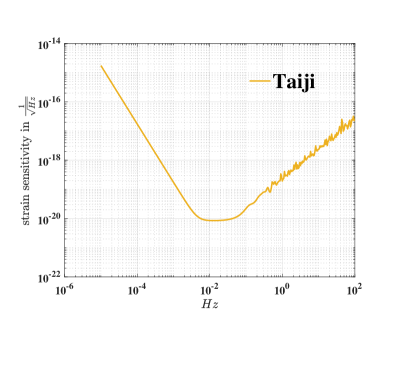
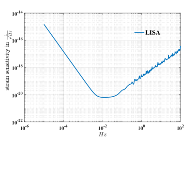
Figure 2: The sensitivity curve of Taiji and LISA. The orange line is the sensitivity curve of Taiji and the blue line is the sensitivity curve of LISA.

By assuming laser frequency noise is sufficiently suppressed in TDI, the acceleration noise and optical path noise are considered to be the dominant noises for GW observation. The budges of acceleration noise for LISA and Taiji are considered as same LISA:2017pwj ; Yang:2022cgm ,

$$S_{\rm acc}=9\ \frac{\rm fm^{2}/s^{4}}{\rm Hz}\left[1+\left(\frac{0.4\ {\rm mHz}}{f}\right)^{2}\right]\left[1+\left(\frac{f}{8\ {\rm mHz}}\right)^{4}\right],$$ (3)

meanwhile, their optical path noise budgets are slightly different as

$$S_{\rm op,LISA} =100\ \frac{\rm pm^{2}}{\rm Hz}\left[1+\left(\frac{2\ {\rm mHz}}{f}\right)^{4}\right],$$ (4)

$$S_{\rm op,Taiji} =64\ \frac{\rm pm^{2}}{\rm Hz}\left[1+\left(\frac{2\ {\rm mHz}}{f}\right)^{4}\right].$$ (5)

The power spectrum density (PSD) of noise which is presented in Fig. 2 is calculated by using the numerical method, see Refs. Wang:2020pkk ; Wang:2020fwa for detailed algorithm.

III.2 Data Curation

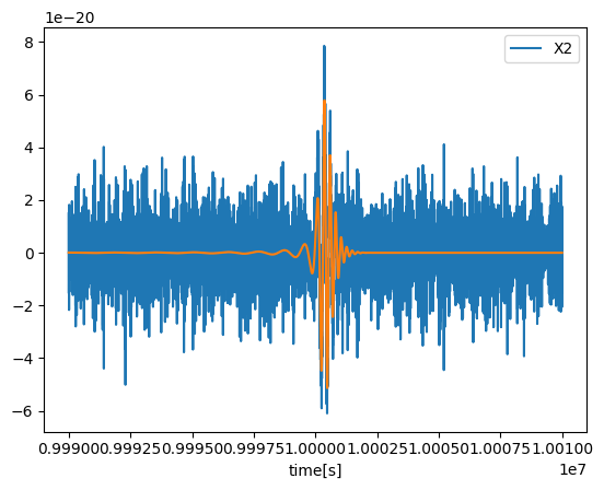
(a) $q=1$, $m_{1}=2\times 10^{6}M_{\odot}$, $m_{2}=2\times 10^{6}M_{\odot}$

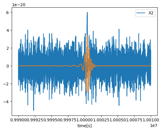
(b) $q=1.5$, $m_{1}=3\times 10^{6}M_{\odot}$, $m_{2}=2\times 10^{6}M_{\odot}$

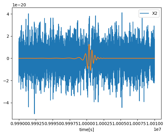
(c) $q=2.5$, $m_{1}=5\times 10^{6}M_{\odot}$, $m_{2}=2\times 10^{6}M_{\odot}$

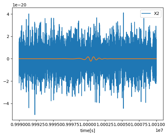
(d) $q=5$, $m_{1}=10^{7}M_{\odot}$, $m_{2}=2\times 10^{6}M_{\odot}$

Figure 3: Time domain representations of the TDI-X channel with different mass ratio $\frac{m_{1}}{m_{2}}=q$. The data from the LDC-2 dataset contain one MBHB signal presented by the orange line, the noise+signal data is presented by the blue line.

We used the signals extracted by the neural network to create new datasets for testing our model’s ability to detect GW signals. The test datasets consisted of 10,000 samples containing signals and 10,000 samples containing only noise. For the MBHB signals, we set the SNR between 30 to 50, and the false alarm rate at $1\%$. For simulated MBHB signals, we used SEOBNRv4_opt, which is a version of the SEOBNRv4 code Bohe:2016gbl with significant optimizations, which can bring the signals for a high spin, high mass ratio MBHB system. We adopted the log-uniform distribution for the parameter $M_{tot}$ from Ref. Katz:2021uax .To facilitate the visual understanding of the signal amplitude and SNR trends, we have presented a time-domain illustration of the waveform in conjunction with the LDC dataset in Fig. 3 and the detailed parameters range is shown in Table 1.

Table 1: Summary of parameter setups in MBHB signal simulation.

Parameter	Lower bound	Upper bound
$M_{tot}$	$10^{6}M_{\odot}$	$10^{8}M_{\odot}$
$q$	$0.1$	$10$
$s_{1}^{z}$	$-0.99$	$0.99$
$s_{2}^{z}$	$-0.99$	$0.99$
$\phi_{0}$	$0$	$2\pi$
$\iota$	$0$	$2\pi$
$\delta$	$0$	$2\pi$

Hereafter, we project the signal to space-based detector, and inject the projected signal to the noise with specific optimal SNR as

$${\rm SNR}=\left(s\mid s\right)^{-1/2},$$ (6)

Here, $s$ represents the signal, and $(h\mid s)$ is

$$(h\mid s)=2\int_{f_{min}}^{f_{max}}\frac{\tilde{h}^{*}(f)\tilde{s}(f)+\tilde{h}(f)\tilde{s}^{*}(f)}{S_{n}(f)}\,df,$$ (7)

where $f_{min}=3\times 10^{-5}{\rm Hz}$ and $f_{max}=0.05{\rm Hz}$, and $S_{n}(f)$ is the noise PSD. Here, following the setting of the LDC-2 dataset and Taiji configuration Ruan:2018tsw ; Ruan:2020smc , we set the SNR to $20$Gair:2022knq . Then the data was whitened and normalized to $[-1,1]$. During the whitening procedure, we applied the Tukey window with $\alpha=1/8$.

IV Results

Our GW twin design comprises two neural networks, Net A for LISA embedding and Net B for Taiji embedding. We concatenate the embeddings and use them as input to the fully connected (FC) layer, where the weights of Net A and Net B are frozen. We only train the FC layer using a subset of the training dataset. Our experiments show that training the FC layer for only 7-8 epochs in TDI-1.0 scenario is sufficient, and we found the same for TDI-1.5 and TDI-2.0 scenarios. Therefore, we choose to consider eight epochs for all three generations.

We evaluate our approach based on five target metrics: AUC score, accuracy score, precision score, recall score, and F1 score. The AUC score reflects the area under the receiver operating characteristic (ROC) curve, which plots the true positive rate (TPR) against the false positive rate (FPR) for all classification thresholds.

$$TPR=\frac{TP}{TP+FN},$$ (8)

where TP stands for“True Positive” and FN stands for“False Negative”,

$$FPR=\frac{FP}{FP+TN},$$ (9)

where FP stands for“False Positive” and TN stands for“True Negative”.

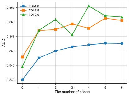
Figure 4: AUC with respect to epoch. The vertical axis represent the value of AUC for SSL model aim at detecting MBHB and the horizontal axis represent the sequence label of epoch.

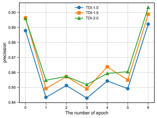
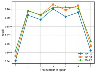
Figure 5: Precision and Recall with respect to epoch under the TDI-1.0(blue), TDI-1.5(orange) and TDI-2.0(green). The vertical axis of the both subfigure represent the value of precision score and the value of recall, the horizontal axis of the both subfigure represent the sequence label of epoch.

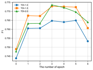
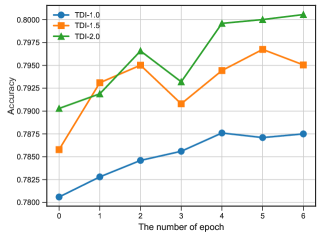
Figure 6: F1 score and accuracy with respect to epoch under the TDI-1.0(blue), TDI-1.5(orange) and TDI-2.0(green). The vertical axis of the both subplotting represent the value of F1 score and the value of accuracy, the horizontal axis of the both subplotting represent the sequence label of epoch.

Fig.4 shows the evolution of AUC values with increasing epoch numbers across TDI-1.0, TDI-1.5, and TDI-2.0 generations. The maximum AUC value ($0.85271$) occurs in the 7th epoch of the TDI-1.0 generation. Interestingly, the AUC value for the 8th epoch is slightly smaller than the 7th epoch, which may be due to overfitting caused by the $1\times 1$ convolution layer between the two epochs. Our results suggest that our self-supervised learning model’s ability to extract MBHB GW signals is sufficient after only 7 epochs of training. In TDI-1.5 and TDI-2.0, the AUC value increases monotonically with an increasing number of training epochs. Notably, the AUC value for TDI-2.0 is greater than TDI-1.5, indicating that our SSL model is more accurate under more realistic TDI assumptions.

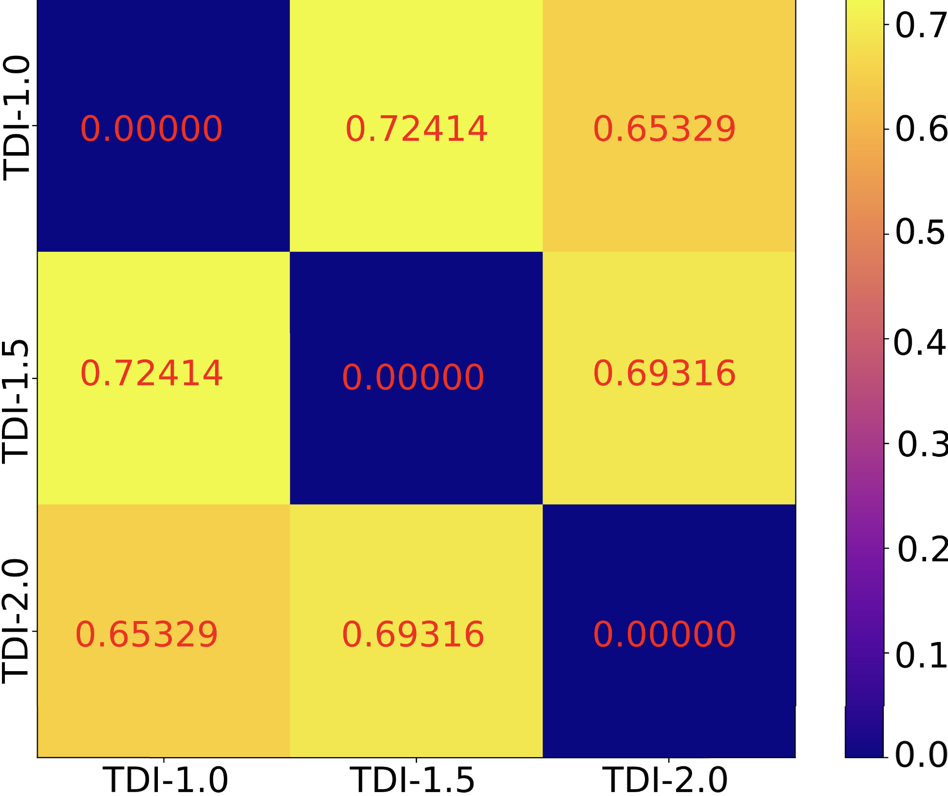
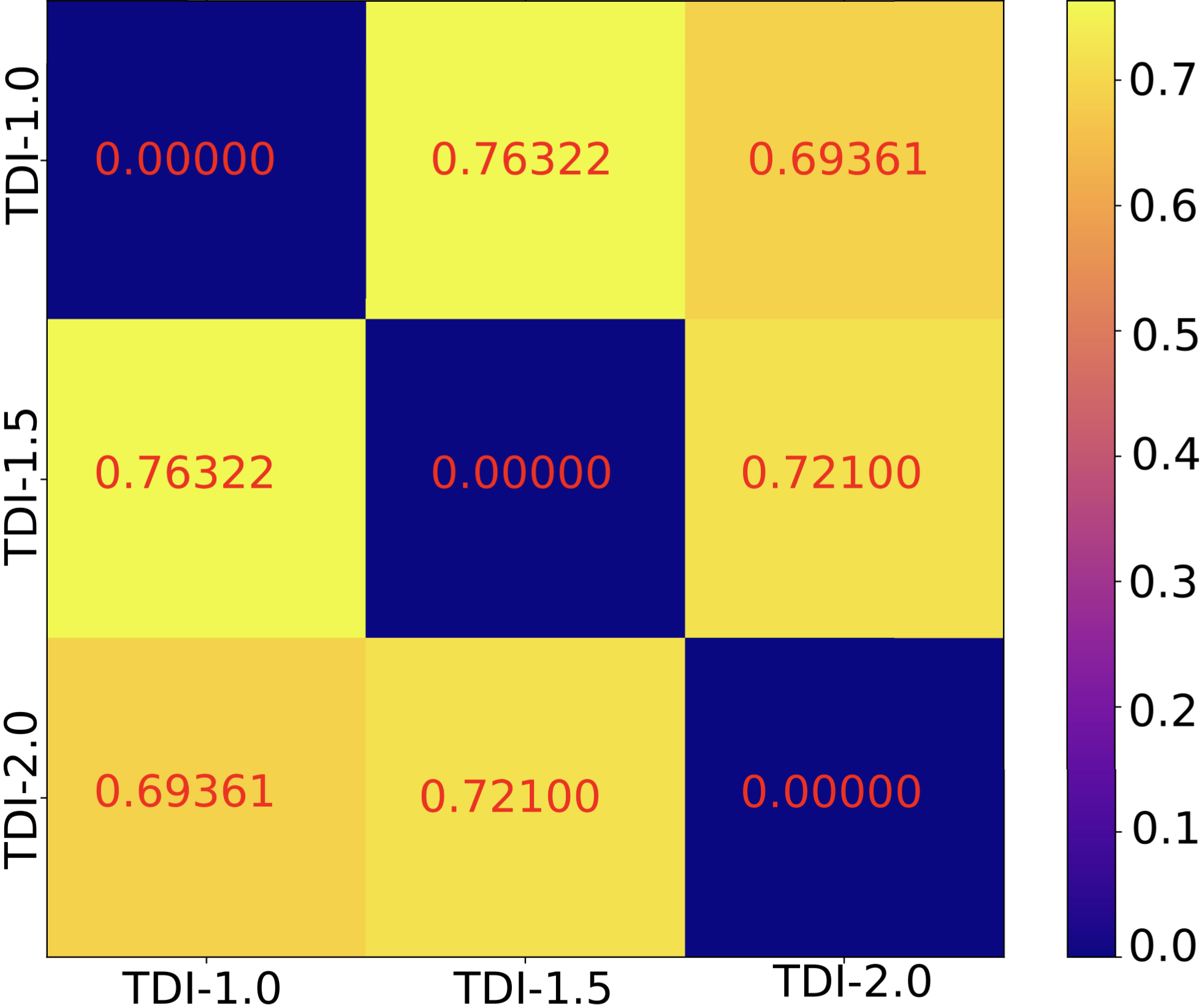
(a) JS divergence for $M_{1}$ and $M_{2}$ marginalization posterior between different TDI generation assumptions with LISA MDC data.

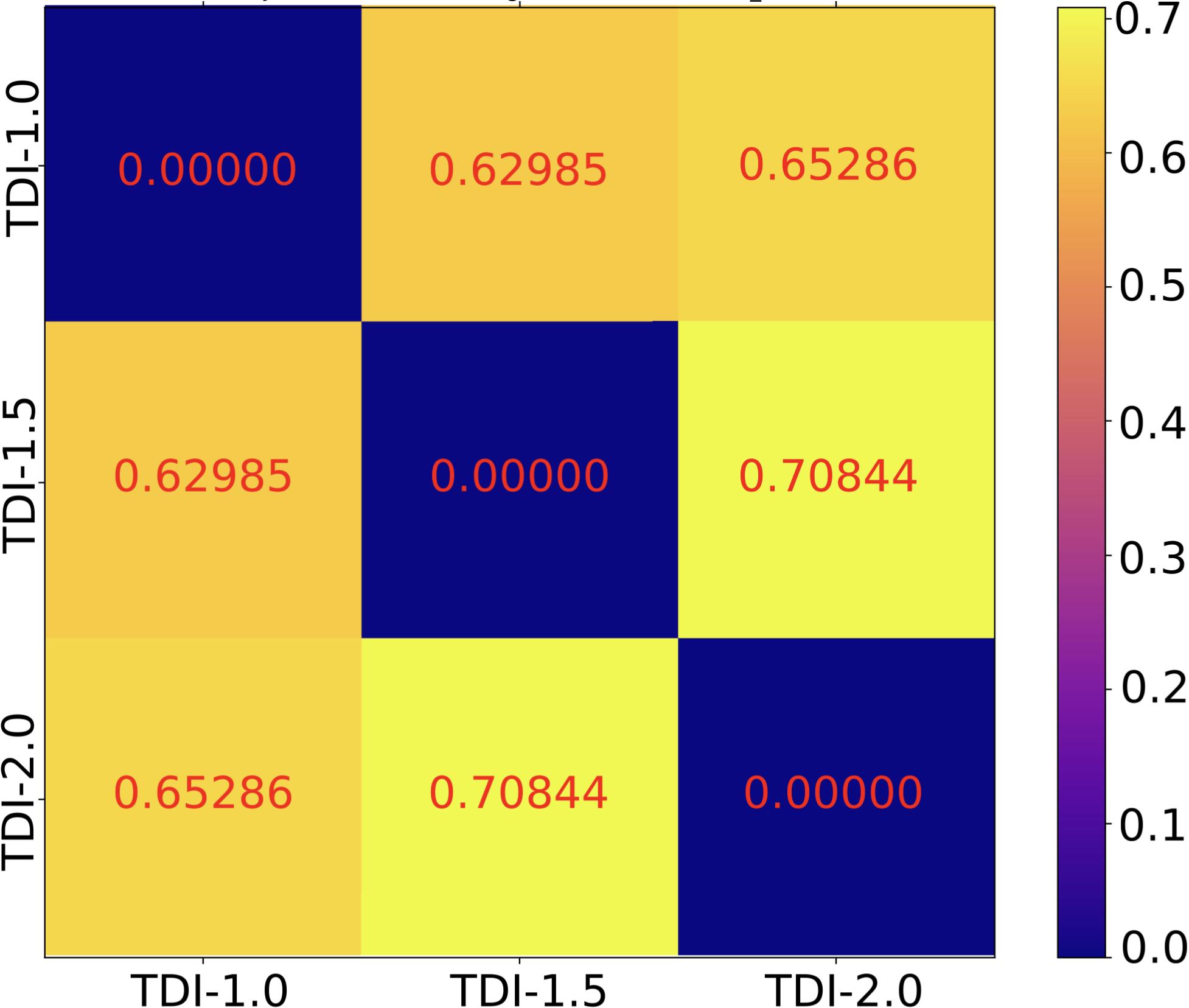
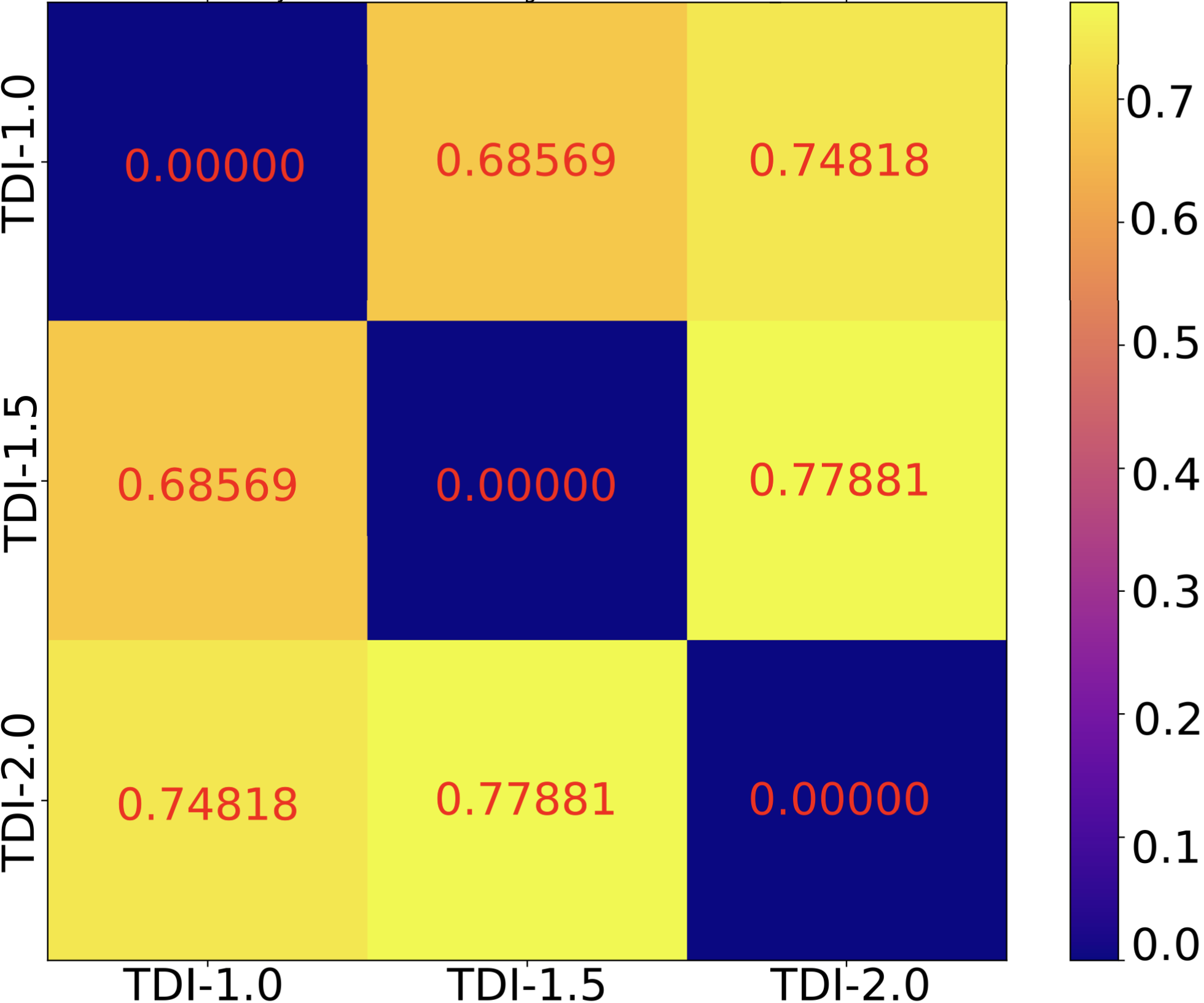
(b) JS divergence for $M_{1}$ and $M_{2}$ marginalization posterior between different TDI generation assumptions with Taiji MDC data.

Figure 7: JSD for primary mass $M_{1}$ and secondary mass $M_{2}$ marginalization posterior between different TDI generation assumption with LISA and Taiji MDC data.

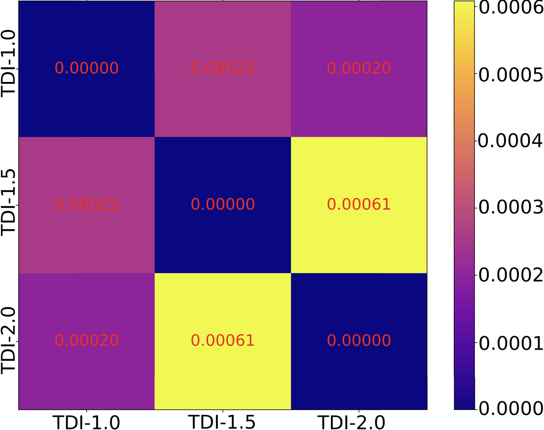
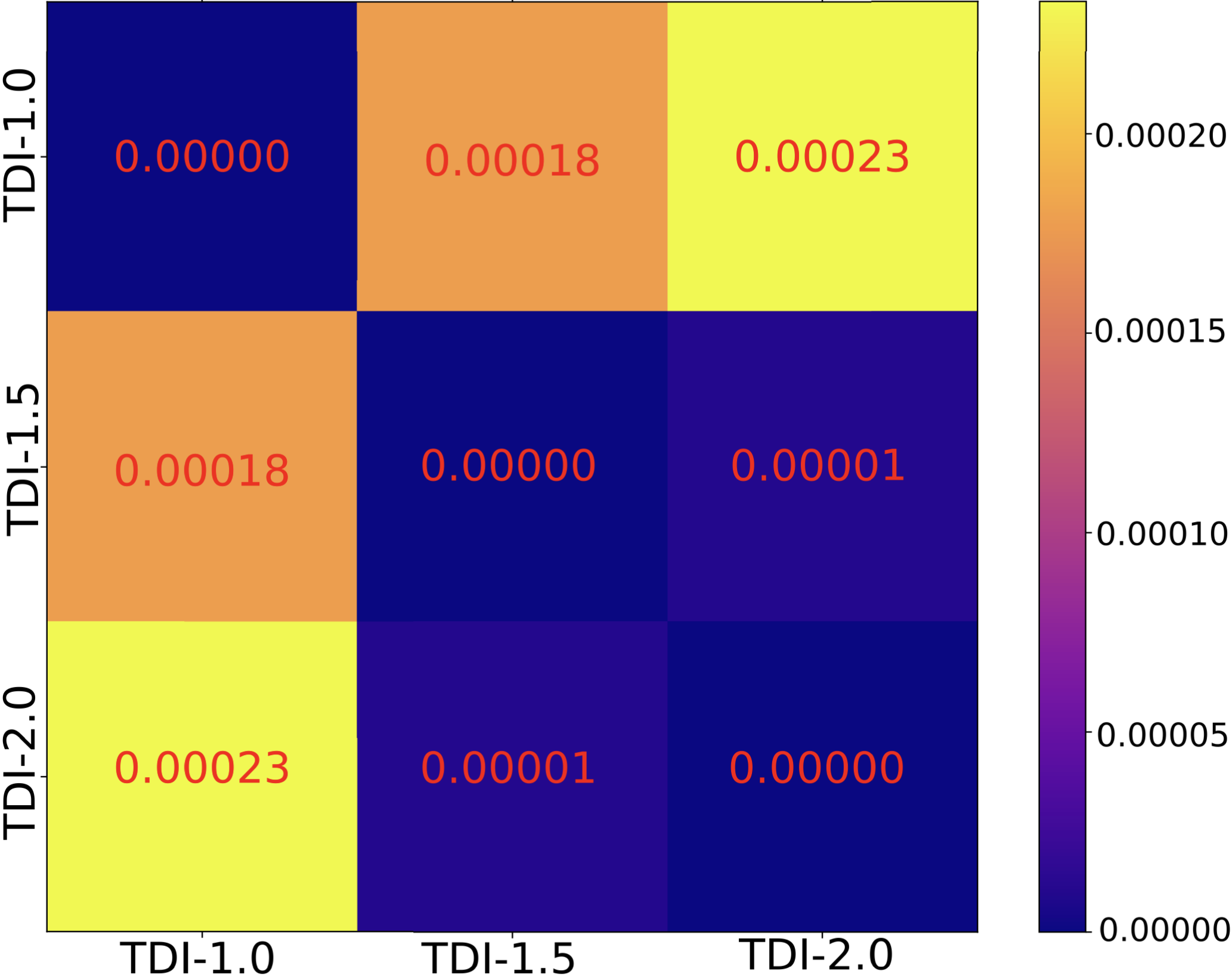
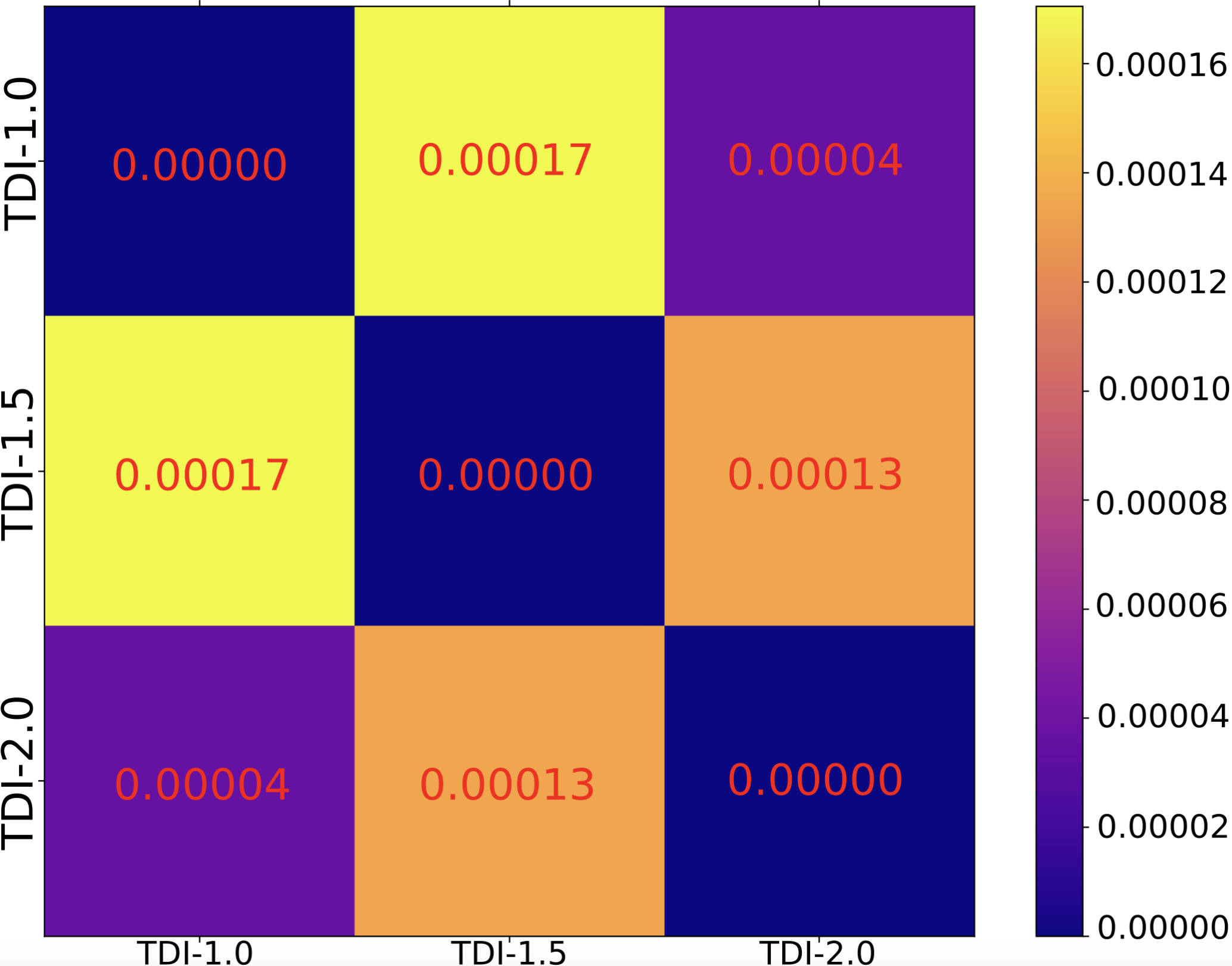
(a) JS divergence for $\phi$, $\iota$ and $\delta$ marginalization posterior between different TDI generation assumptions with LISA MDC data.

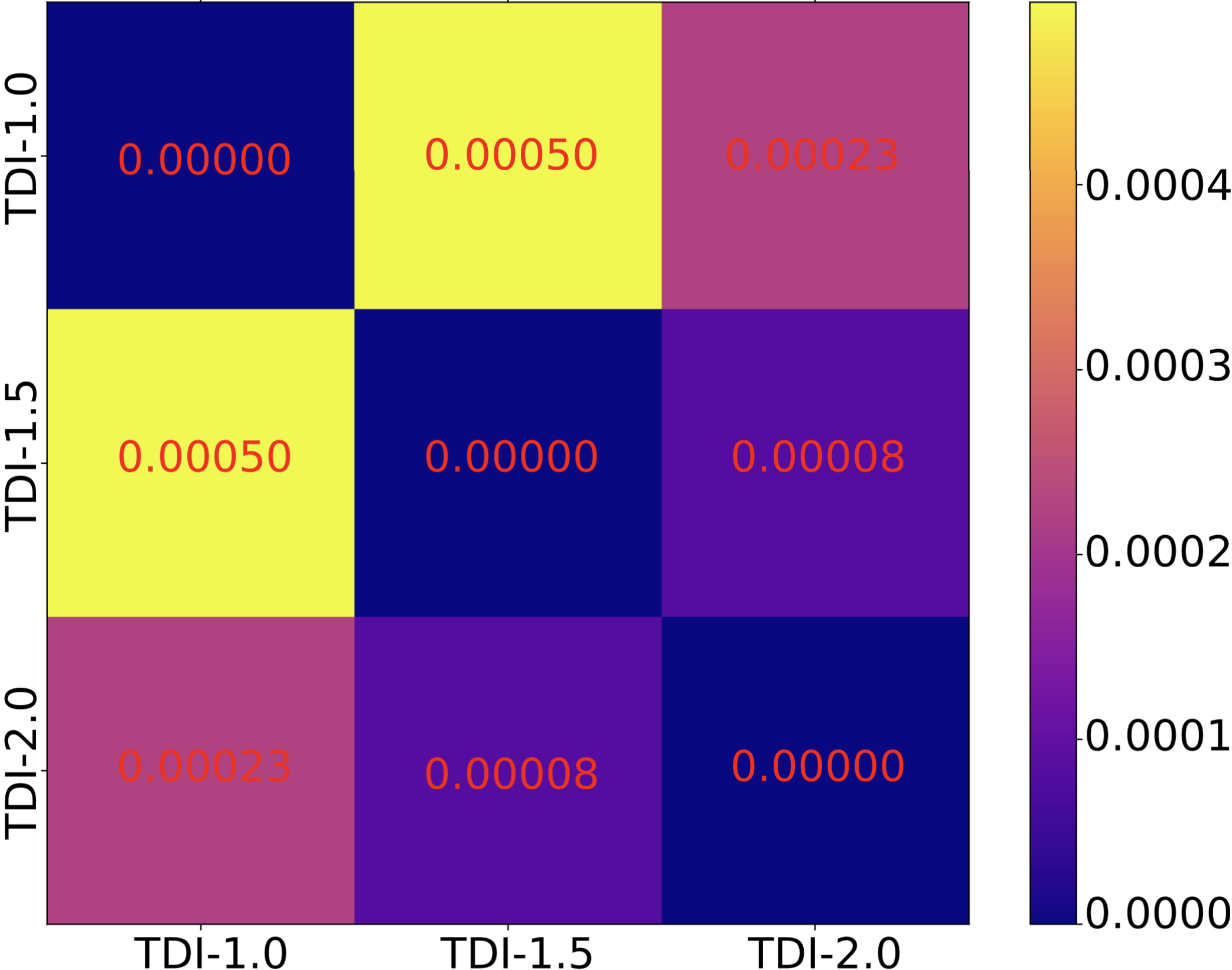
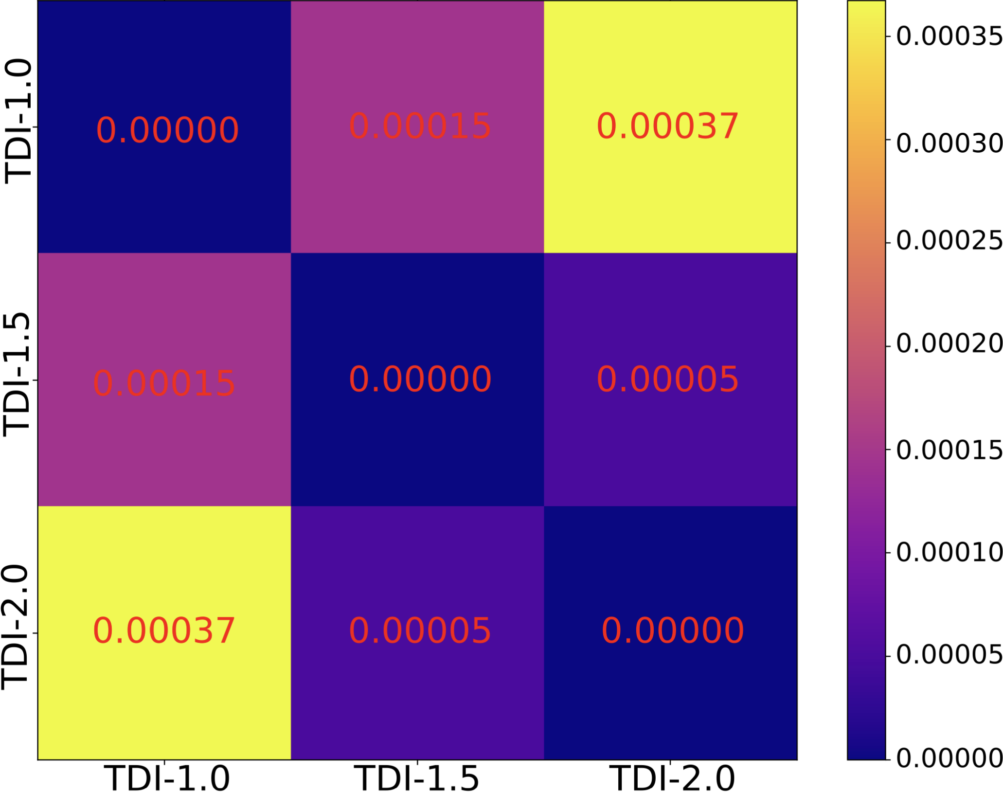
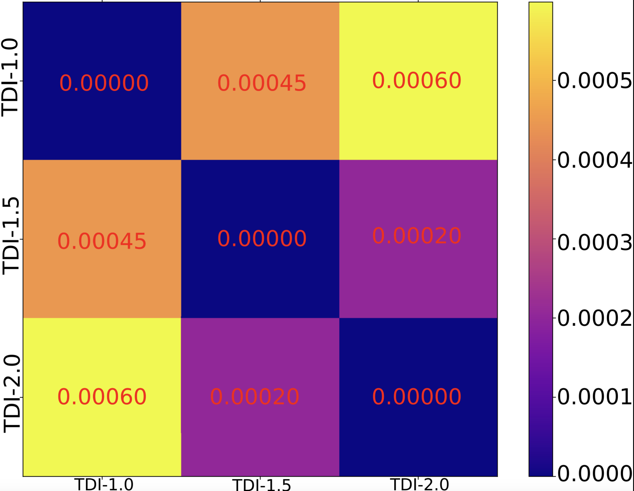
(b) JS divergence for $\phi$, $\iota$ and $\delta$ marginalization posterior between different TDI generation assumptions with Taiji MDC data.

Figure 8: JSD for phase $\phi$, inclination angle $\iota$ and polarization angle $\delta$ marginalization posterior between different TDI generation assumption with LISA and Taiji MDC data.

We also show the precision and recall. The Precision attempts to describe the proportion of actually correct positive identifications,

$$Precision=\frac{TP}{TP+FP}.$$ (10)

The Recall describes the proportion of identified correctly actual positives,

$$Recall=\frac{TP}{TP+FN},$$ (11)

Our model achieves high Precision scores in the 7th epoch, suggesting correct detection of GW signals by our self-supervised learning model. The relatively high Recall rate indicates a relatively low rate of false negatives; however, precision and recall are often in tension such that improving one typically reduces the other. To evaluate the effectiveness of our model, we analyze both precision and recall, and utilize the F1 score to provide a holistic assessment in signal retrieval. The F1 score is a frequently-used metric in machine learning that evaluates the performance of binary classification models by balancing precision and recall. We define the F1 score using the equation:

$$F1=\frac{2TP}{2TP+FP+FN},$$ (12)

In addition to the F1 score, we also calculate Accuracy, a widely used evaluation metric for classification models. Informally, accuracy measures the fraction of correct predictions made by our model and is defined as:

$$Accuracy=\frac{TP+TN}{TP+TN+FP+FN}.$$ (13)

In Figure 6, we show the changes in F1 score and accuracy with respect to epoch number. Both metrics steadily increase, indicating that our self-supervised learning (SSL) approach supports good generalization for Massive Binary Black Hole (MBHB) signal searching under any Time Delay Interferometry (TDI) generation assumption, from a holistic perspective. We also observe that the F1 score and accuracy levels are similar, suggesting that our SSL model is capable of handling imbalanced data, which is a significant advantage of SSL.

We investigate the effect of different TDI generations on the SSL method’s performance in estimating five key parameters ( $M_{1}$, $M_{2}$, $\phi$, $\iota$, $\delta$), using a modified DINGO-GW code packageGW:DINGO based on the neural parameter estimation (NPE) method. Our analysis uses data that we trained with our SSL method, and we evaluate the influence of different TDI generations using the Jenson-Shannon (JS) divergence metric. Smaller JS divergence values indicate that parameter estimations for different TDI generations are comparable, supporting our inference that the SSL method is minimally influenced by the TDI generation assumptions. As seen in Figure.7, the influence of different TDI generation assumptions on the primary and secondary mass is significant in both the LISA and Taiji MDC datasets. However, as Figure.8 shows, the effect on $\phi$, $\iota$ and $\delta$ in both datasets is negligible. This is because the SNR of the MBHB signal is most strongly influenced by changes in primary and secondary mass, while the contribution from phase and skymap localization angle is minor. Therefore, despite the influence of TDI generation assumptions on mass, the SSL method’s performance in estimating $\phi$, $\iota$ and $\delta$ remains consistent across different TDI generations.

SSL also offers significant computational efficiency advantages over other methods. To demonstrate this, we compare SSL to the Long Short-Term Memory network (LSTM)Hochreiter:1997yld and LDASoftLDA:LDASoft methods on the LISA and Taiji MDC datasets. Using all three methods, we search for specific injection signals and evaluate the time costs of each. Figure 9 shows that LDASoft incurs the highest time cost among the three methods in the LISA MDC data environment, steadily increasing as TDI configuration approaches the true value. Conversely, SSL and LSTM significantly reduce time costs by over 70% as compared to LDASoft, with SSL being the most efficient. The annotation costs and overall computational costs are also lower with SSL. We believe that further methodological enhancements and the availability of more robust training organizations will make SSL even more promising for controlling computational costs.

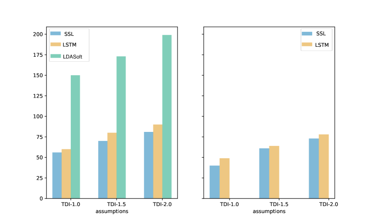
Figure 9: We compare the time cost for three methods - SSL (blue histogram), LSTM (yellow histogram), and LDASoft (green histogram) - for different TDI generations. The left plot displays the results for LISA MDC data, where we compare the time cost of the three main methods. The right plot shows the results for TAIJI MDC data, where we compare the time cost of both machine learning methods.

V Conclusion

In this paper, we present a self-supervised learning model for GW detection. Our model is based on simulated massive black hole binary signals embedded in synthetic Gaussian noise that matches space-based GW detectors’ Taiji and LISA sensitivity. Our results demonstrate that the self-supervised learning model we propose is capable of extracting signals and that it is a highly efficient method for GW signal identification.

To accomplish this, we utilize a corresponding contrastive learning method in which we propose the GW twins design operating on a joint embedding of augmentation vectors (where Net A and Net B represent the LISA and Taiji embeddings, respectively). This design is conceptually simple, easy to implement, and benefits from high-dimensional embeddings that do not require large batches, asymmetric mechanisms such as momentum encoders or non-differentiable operators, or stop-gradients.

We apply our SSL method to a simple signal search scenario in which we search for MBHB signals in detecting data. Our results show that the SSL method does well in recovering the injected MBHB signals from the Gaussian noise with both the LISA MDC and Taiji data settings. From various metric results, we conclude that SSL is more effective with a more realistic TDI generation assumption from an entire angle, and the different TDI generations can influence the primary mass and secondary mass inference results obviously and slightly for $\phi$, $\iota$ and $\delta$ when using the SSL method. The time cost of SSL is advantageous to LDASoft based on globalfit, and it also uses less computation cost than the LSTM method. It will reduce the computation cost and time with future optimizations.

Although we applied our method to the MBHB GW events, it could still be applied to other cases, such as binary white dwarf and extreme mass ratio inspirals. It might be helpful in searching for the GW echo signals, particularly the unequal interval echoes Wang:2018mlp ; Wang:2018cum ; Li:2019kwa . The search for signals in GW data is mainly affected by non-Gaussian noise. Actually, our method can be applied in realistic non-Gaussian data. Note that the claim of matched-filtering optimality only applies in the Gaussian noise case. We will study these interesting issues in later works.

It is worth mentioning that we take Taiji and LISA as GW twins to present our method; however, self-supervised learning can also be applied in land-based GW detectors with high-quality dataLIGO:2021ppb ; Virgo:2022fxr ; Virgo:2022ysc .

VI Acknowledgments

WYT is supported by National Key Research and Development Program of China Grant No. 2021YFC2203004. We acknowledge the Tianhe-2 supercomputer for providing computing resources.

References

- (1) B. P. Abbott et al. [LIGO Scientific and Virgo], Phys. Rev. Lett. 116, no.6, 061102 (2016) doi:10.1103/PhysRevLett.116.061102 [arXiv:1602.03837 [gr-qc]].
- (2) B. P. Abbott et al. [LIGO Scientific and Virgo], Phys. Rev. Lett. 116, no.24, 241103 (2016) doi:10.1103/PhysRevLett.116.241103 [arXiv:1606.04855 [gr-qc]].
- (3) B. P. Abbott et al. [LIGO Scientific and VIRGO], Phys. Rev. Lett. 118, no.22, 221101 (2017) [erratum: Phys. Rev. Lett. 121, no.12, 129901 (2018)] doi:10.1103/PhysRevLett.118.221101 [arXiv:1706.01812 [gr-qc]].
- (4) B. P. Abbott et al. [LIGO Scientific and Virgo], Phys. Rev. Lett. 119, no.16, 161101 (2017) doi:10.1103/PhysRevLett.119.161101 [arXiv:1710.05832 [gr-qc]].
- (5) B. P. Abbott et al. [LIGO Scientific and Virgo], Phys. Rev. X 9, no.3, 031040 (2019) doi:10.1103/PhysRevX.9.031040 [arXiv:1811.12907 [astro-ph.HE]].
- (6) R. Abbott et al. [LIGO Scientific and Virgo], Phys. Rev. X 11, 021053 (2021) doi:10.1103/PhysRevX.11.021053 [arXiv:2010.14527 [gr-qc]].
- (7) R. Abbott et al. [LIGO Scientific, VIRGO and KAGRA], [arXiv:2111.03606 [gr-qc]].
- (8) D. A. Brown, I. Harry, A. Lundgren and A. H. Nitz, Phys. Rev. D 86, 084017 (2012) doi:10.1103/PhysRevD.86.084017 [arXiv:1207.6406 [gr-qc]].
- (9) T. Dal Canton and I. W. Harry, [arXiv:1705.01845 [gr-qc]].
- (10) I. W. Harry, B. Allen and B. S. Sathyaprakash, Phys. Rev. D 80, 104014 (2009) doi:10.1103/PhysRevD.80.104014 [arXiv:0908.2090 [gr-qc]].
- (11) T. Dal Canton, A. H. Nitz, A. P. Lundgren, A. B. Nielsen, D. A. Brown, T. Dent, I. W. Harry, B. Krishnan, A. J. Miller and K. Wette, et al. Phys. Rev. D 90, no.8, 082004 (2014) doi:10.1103/PhysRevD.90.082004 [arXiv:1405.6731 [gr-qc]].
- (12) P. Ajith, N. Fotopoulos, S. Privitera, A. Neunzert and A. J. Weinstein, Phys. Rev. D 89, no.8, 084041 (2014) doi:10.1103/PhysRevD.89.084041 [arXiv:1210.6666 [gr-qc]].
- (13) B. S. Sathyaprakash and S. V. Dhurandhar, Phys. Rev. D 44, 3819-3834 (1991) doi:10.1103/PhysRevD.44.3819
- (14) A. Taracchini, A. Buonanno, Y. Pan, T. Hinderer, M. Boyle, D. A. Hemberger, L. E. Kidder, G. Lovelace, A. H. Mroué and H. P. Pfeiffer, et al. Phys. Rev. D 89, no.6, 061502 (2014) doi:10.1103/PhysRevD.89.061502 [arXiv:1311.2544 [gr-qc]].
- (15) S. Privitera, S. R. P. Mohapatra, P. Ajith, K. Cannon, N. Fotopoulos, M. A. Frei, C. Hanna, A. J. Weinstein and J. T. Whelan, Phys. Rev. D 89, no.2, 024003 (2014) doi:10.1103/PhysRevD.89.024003 [arXiv:1310.5633 [gr-qc]].
- (16) L. Blanchet, Living Rev. Rel. 17, 2 (2014) doi:10.12942/lrr-2014-2 [arXiv:1310.1528 [gr-qc]].
- (17) K. G. Arun, A. Buonanno, G. Faye and E. Ochsner, Phys. Rev. D 79, 104023 (2009) [erratum: Phys. Rev. D 84, 049901 (2011)] doi:10.1103/PhysRevD.79.104023 [arXiv:0810.5336 [gr-qc]].
- (18) A. Buonanno, B. Iyer, E. Ochsner, Y. Pan and B. S. Sathyaprakash, Phys. Rev. D 80, 084043 (2009) doi:10.1103/PhysRevD.80.084043 [arXiv:0907.0700 [gr-qc]].
- (19) C. K. Mishra, A. Kela, K. G. Arun and G. Faye, Phys. Rev. D 93, no.8, 084054 (2016) doi:10.1103/PhysRevD.93.084054 [arXiv:1601.05588 [gr-qc]].
- (20) A. Buonanno and T. Damour, Phys. Rev. D 59, 084006 (1999) doi:10.1103/PhysRevD.59.084006 [arXiv:gr-qc/9811091 [gr-qc]].
- (21) F. Pretorius, Phys. Rev. Lett. 95, 121101 (2005) doi:10.1103/PhysRevLett.95.121101 [arXiv:gr-qc/0507014 [gr-qc]].
- (22) I. J. Goodfellow, J. Pouget-Abadie, M. Mirza, B. Xu, D. Warde-Farley, S. Ozair, A. Courville and Y. Bengio, [arXiv:1406.2661 [stat.ML]].
- (23) K. Simonyan and A. Zisserman, [arXiv:1409.1556 [cs.CV]].
- (24) Liang-Chieh Chen, George Papandreou, Iasonas Kokkinos, Kevin Murphy, Alan L. Yuille [arXiv:1412.7062 [cs.CV]].
- (25) Matthew D Zeiler, Rob Fergus [arXiv:1311.2901 [cs.CV]].
- (26) C. Szegedy, W. Liu, Y. Jia, P. Sermanet, S. Reed, D. Anguelov, D. Erhan, V. Vanhoucke and A. Rabinovich, [arXiv:1409.4842 [cs.CV]].
- (27) R. Zhang, P. Isola, A. A. Efros, [arXiv:1603.08511 [cs.CV]].
- (28) Andrej Karpathy, Li Fei-Fei [arXiv:1412.2306 [cs.CV]].
- (29) N. Mukund, S. Abraham, S. Kandhasamy, S. Mitra and N. S. Philip, Phys. Rev. D 95, no.10, 104059 (2017) doi:10.1103/PhysRevD.95.104059 [arXiv:1609.07259 [astro-ph.IM]].
- (30) M. Zevin, S. Coughlin, S. Bahaadini, E. Besler, N. Rohani, S. Allen, M. Cabero, K. Crowston, A. Katsaggelos and S. Larson, et al. Class. Quant. Grav. 34, no.6, 064003 (2017) doi:10.1088/1361-6382/aa5cea [arXiv:1611.04596 [gr-qc]].
- (31) D. George, H. Shen and E. A. Huerta, [arXiv:1706.07446 [gr-qc]].
- (32) D. George and E. A. Huerta, Phys. Rev. D 97, no.4, 044039 (2018) doi:10.1103/PhysRevD.97.044039 [arXiv:1701.00008 [astro-ph.IM]].
- (33) W. Wei and E. A. Huerta, Phys. Lett. B 800, 135081 (2020) doi:10.1016/j.physletb.2019.135081 [arXiv:1901.00869 [gr-qc]].
- (34) H. Xia, L. Shao, J. Zhao and Z. Cao, Phys. Rev. D 103, no.2, 024040 (2021) doi:10.1103/PhysRevD.103.024040 [arXiv:2011.04418 [astro-ph.HE]].
- (35) Y. C. Lin and J. H. P. Wu, Phys. Rev. D 103, no.6, 063034 (2021) doi:10.1103/PhysRevD.103.063034 [arXiv:2007.04176 [astro-ph.IM]].
- (36) C. H. Liao and F. L. Lin, Phys. Rev. D 103, no.12, 124051 (2021) doi:10.1103/PhysRevD.103.124051 [arXiv:2101.06685 [astro-ph.IM]].
- (37) W. H. Ruan, H. Wang, C. Liu and Z. K. Guo, [arXiv:2111.14546 [astro-ph.IM]].
- (38) P. Bacon, A. Trovato and M. Bejger, [arXiv:2205.13513 [gr-qc]].
- (39) T. Zhao, R. Lyu, Z. Ren, H. Wang and Z. Cao, [arXiv:2207.07414 [gr-qc]].
- (40) M. B. Schäfer, O. Zelenka, A. H. Nitz, H. Wang, S. Wu, Z. K. Guo, Z. Cao, Z. Ren, P. Nousi and N. Stergioulas, et al. [arXiv:2209.11146 [astro-ph.IM]].
- (41) C. Murali and D. Lumley, [arXiv:2210.01718 [gr-qc]].
- (42) P. Nousi, A. E. Koloniari, N. Passalis, P. Iosif, N. Stergioulas and A. Tefas, [arXiv:2211.01520 [gr-qc]].
- (43) H. Shen, E. A. Huerta, E. O’Shea, P. Kumar and Z. Zhao, Mach. Learn. Sci. Tech. 3, no.1, 015007 (2022) doi:10.1088/2632-2153/ac3843 [arXiv:1903.01998 [gr-qc]].
- (44) Z. Ren, H. Wang, Y. Zhou, Z. K. Guo and Z. Cao, [arXiv:2212.14283 [gr-qc]].
- (45) T. Chen, S. Kornblith, M. Norouzi, G. Hinton, [arXiv:2002.05709 [cs.LG]].
- (46) I. Misra, L. Maaten, [arXiv:1912.01991 [cs.CV]].
- (47) J. Zbontar, L. Jing, I. Misra, Y. LeCun, S. Deny, [arXiv:2103.03230 [cs.CV]].
- (48) W. R. Hu and Y. L. Wu, Natl. Sci. Rev. 4, no.5, 685-686 (2017) doi:10.1093/nsr/nwx116
- (49) P. Amaro-Seoane et al. [LISA], [arXiv:1702.00786 [astro-ph.IM]].
- (50) https://lisa-ldc.lal.in2p3.fr
- (51) http://taiji-tdc.ictp-ap.org
- (52) N. Tishby, F. C. Pereira, W. Bialek [arXiv:physics/0004057].
- (53) N. Tishby, N. Zaslavsky, [arXiv:1503.02406 [cs.LG]].
- (54) A. van den Oord, Y. Z. Li, O. Vinyals, [arXiv:1807.03748[cs.LG]].
- (55) Y. You, I. Gitman, B. Ginsburg, [arXiv:1708.03888 [cs.CV]].
- (56) M. Otto, G. Heinzel and K. Danzmann, Class. Quant. Grav. 29, 205003 (2012) doi:10.1088/0264-9381/29/20/205003
- (57) M. Otto, doi:10.15488/8545
- (58) M. Tinto and O. Hartwig, Phys. Rev. D 98, no.4, 042003 (2018) doi:10.1103/PhysRevD.98.042003 [arXiv:1807.02594 [gr-qc]].
- (59) G. Wang, W. T. Ni, W. B. Han and C. F. Qiao, Phys. Rev. D 103, no.12, 122006 (2021) doi:10.1103/PhysRevD.103.122006 [arXiv:2010.15544 [gr-qc]].
- (60) G. Wang and W. T. Ni, [arXiv:2008.05812 [gr-qc]].
- (61) G. Wang and W. B. Han, Phys. Rev. D 103, no.6, 064021 (2021) doi:10.1103/PhysRevD.103.064021 [arXiv:2101.01991 [gr-qc]].
- (62) T. A. Prince, M. Tinto, S. L. Larson and J. W. Armstrong, Phys. Rev. D 66, 122002 (2002) doi:10.1103/PhysRevD.66.122002 [arXiv:gr-qc/0209039 [gr-qc]].
- (63) M. Vallisneri, J. Crowder and M. Tinto, Class. Quant. Grav. 25, 065005 (2008) doi:10.1088/0264-9381/25/6/065005 [arXiv:0710.4369 [gr-qc]].
- (64) Y. Yang, W. B. Han, Q. Yun, P. Xu and Z. Luo, Mon. Not. Roy. Astron. Soc. 512, no.4, 6217-6224 (2022) doi:10.1093/mnras/stac920 [arXiv:2205.00408 [gr-qc]].
- (65) A. Bohé, L. Shao, A. Taracchini, A. Buonanno, S. Babak, I. W. Harry, I. Hinder, S. Ossokine, M. Pürrer and V. Raymond, et al. Phys. Rev. D 95, no.4, 044028 (2017) doi:10.1103/PhysRevD.95.044028 [arXiv:1611.03703 [gr-qc]].
- (66) https://github.com/dingo-gw/dingo
- (67) S. Hochreiter and J. Schmidhuber, Neural Comput. 9, no.8, 1735-1780 (1997) doi:10.1162/neco.1997.9.8.1735
- (68) https://github.com/tlittenberg/ldasoft
- (69) M. L. Katz, Phys. Rev. D 105, no.4, 044055 (2022) doi:10.1103/PhysRevD.105.044055 [arXiv:2111.01064 [gr-qc]].
- (70) W. H. Ruan, Z. K. Guo, R. G. Cai and Y. Z. Zhang, Int. J. Mod. Phys. A 35, no.17, 2050075 (2020) doi:10.1142/S0217751X2050075X [arXiv:1807.09495 [gr-qc]].
- (71) W. H. Ruan, C. Liu, Z. K. Guo, Y. L. Wu and R. G. Cai, Nature Astron. 4, 108-109 (2020) doi:10.1038/s41550-019-1008-4 [arXiv:2002.03603 [gr-qc]].
- (72) J. R. Gair, M. Hewitson, A. Petiteau and G. Mueller, “Space-based Gravitational Wave Observatories,” doi:10.1007/978-981-15-4702-7_3-1 [arXiv:2201.10593 [gr-qc]].
- (73) Y. T. Wang, Z. P. Li, J. Zhang, S. Y. Zhou and Y. S. Piao, Eur. Phys. J. C 78 (2018) no.6, 482 doi:10.1140/epjc/s10052-018-5974-y [arXiv:1802.02003 [gr-qc]].
- (74) Y. T. Wang, J. Zhang and Y. S. Piao, Phys. Lett. B 795 (2019), 314-318 doi:10.1016/j.physletb.2019.06.036 [arXiv:1810.04885 [gr-qc]].
- (75) Z. P. Li and Y. S. Piao, Phys. Rev. D 100 (2019) no.4, 044023 doi:10.1103/PhysRevD.100.044023 [arXiv:1904.05652 [gr-qc]].
- (76) D. Davis et al. [LIGO], Class. Quant. Grav. 38, no.13, 135014 (2021) doi:10.1088/1361-6382/abfd85 [arXiv:2101.11673 [astro-ph.IM]].
- (77) F. Acernese et al. [Virgo], [arXiv:2205.01555 [gr-qc]].
- (78) F. Acernese et al. [Virgo], [arXiv:2210.15633 [gr-qc]].