W2SAT: Learning to generate SAT instances from
Weighted Literal Incidence Graphs

Abstract

The Boolean Satisfiability (SAT) problem stands out as an attractive NP-complete problem in theoretic computer science and plays a central role in a broad spectrum of computing-related applications. Exploiting and tuning SAT solvers under numerous scenarios require massive high-quality industry-level SAT instances, which unfortunately are quite limited in the real world. To address the data insufficiency issue, in this paper, we propose W2SAT, a framework to generate SAT formulas by learning intrinsic structures and properties from given real-world/industrial instances in an implicit fashion. To this end, we introduce a novel SAT representation called Weighted Literal Incidence Graph (WLIG), which exhibits strong representation ability and generalizability against existing counterparts, and can be efficiently generated via a specialized learning-based graph generative model. Decoding from WLIGs into SAT problems is then modeled as finding overlapping cliques with a novel hill-climbing optimization method termed Optimal Weight Coverage (OWC). Experiments demonstrate the superiority of our WLIG-induced approach in terms of graph metrics, efficiency, and scalability in comparison to previous methods. Additionally, we discuss the limitations of graph-based SAT generation for real-world applications, especially when utilizing generated instances for SAT solver parameter-tuning, and pose some potential directions.

1 Introduction

The Boolean Satisfiability (SAT) problem asks whether a given boolean formula has a 0/1-assignment of literals therein, such that this formula can be evaluated to true. Despite its succinctness, SAT is the first problem proved NP-complete (Cook, 1971) and has grounded as a fundamental to a large variety of real-world and industrial applications ranging from software verification (Clarke et al., 2001) and electronic design automation (EDA) (Marques-Silva & Sakallah, 2000), to planning (Kautz et al., 1992) and theorem proving (Ganzinger et al., 2004). Although it is believed that there is no polynomial-time algorithm to SAT solving, various solvers are proposed taking into account some specific aspects (e.g., distribution, structure, and modularity) of SAT problems, achieving impressive efficiency and performance in practice. According to this, some successful research investigate automatic solver selection by identifying different structures of SAT instances (Xu et al., 2012; Ansótegui et al., 2017). This fact demonstrates that the exploitation and development of solvers can be potentially improved once structures/representations of different SAT instances are well understood and captured.

As such, researchers have been persistently focusing on developing and evaluating better solvers by inspecting the intrinsic structures/representations of SAT instances from different fields, which calls for a large amount of real-world or industry-level SAT formulas. Although enlarged SAT benchmarks are becoming available in different areas (Hoos & Stützle, 2000; Aloul et al., 2003), they are still in shortage in comparison to the increasing demand for the development and evaluation of SAT solvers. For example, in industry one may need to evaluate and design solvers for circuits with specific functionalities, yet the number of circuits is quite limited. A natural way of addressing the insufficiency issue is to generate instances that resemble the characteristics of a given set of SAT problems.

To better capture the structure of SAT, some works put forward SAT generation via graph representations (Giráldez-Cru & Levy, 2015, 2017; You et al., 2019; Garzón et al., 2022; Wu & Ramanujan, 2019), as graphs are believed to carry rich structural information with high applicability of modeling. In general, these representations can be categorized into 1) inexact: literal-incidence graph (LIG), variable-incidence graph (VIG), and variable-clause graph (VCG), which represent SAT formulas with information loss, so that different formulas may be encoded into an identical graph; or 2) exact: literal-clause graph (LCG), which is equivalent to its original formula. Wu & Ramanujan (2019) argued that despite the exactness, LCG is challenging to learn/generate and to be extended to a large scale, which in turn was shown by You et al. (2019); Garzón et al. (2022). However, approximate representations may miss too much structural information about the original formula, yielding weak representation ability (Giráldez-Cru & Levy, 2015, 2017; Wu & Ramanujan, 2019).

In this paper, we introduce a novel graph-level representation for SAT – Weighted Literal Incidence Graphs (WLIGs) – which allows for strong representation ability w.r.t. SAT without sacrificing its learning and generation efficiency. As its name shows, WLIG differs from LIG only by encoding extra strength of literal incidence as weights on edges. See Fig. 1 for an example. With this slight modification, we argue that WLIG is capable of carrying much richer structural and contextual information (e.g., importance of literals, co-occurrence frequency) than LIG (Wu & Ramanujan, 2019). In addition, learning and generating SAT instances can be efficiently achieved with strong scalability in the WLIG implicit space, which is extremely hard in LCG space (You et al., 2019; Garzón et al., 2022).

Having WLIGs by hand, we still face two essential questions: How to learn from given WLIGs (representing SAT instances) and generate new ones? How to decode a WLIG into a SAT formula? For the first question, we draw inspiration from CELL (Rendsburg et al., 2020), a spectral-theory-driven efficient graph generation method for unweighted graphs. We adapt CELL to weighted graphs by incorporating an incidence strength prediction procedure for generated edges, without sacrificing the generation efficiency. For the second question, we developed a specialized hill-climbing-inspired algorithm called Optimal Weight Coverage (OWC), by regarding the decoding procedure as finding most likely overlapping cliques termed Weighted Clique Edge Cover (WCEC) problem in WLIGs.

Altogether, we present W2SAT, an efficient and scalable SAT instance generation framework. The overview of W2SAT can be found in Fig. 2. Given a SAT formula, W2SAT learns to sample a collection of pseudo-instances by imitating global and local properties of the original one, following the setting in (Wu & Ramanujan, 2019). We experimentally show that, compared to prior arts, W2SAT achieved superior performance in terms of graph metrics, learning and generation efficiency, and scalability. Furthermore, we discuss the limitation of parameter tuning for SAT solvers using graph-based generators. Here we summarize the contributions of this work as follows:

• We proposed a novel graph representation of SAT problem namely WLIG, which balances the representation ability and the learning/generating efficiency.

• We developed a specialized algorithm OWC, to efficiently recover WLIG into SAT formula by inferring overlapping cliques in a hill-climbing fashion.

• We presented W2SAT, a real-world and industrial SAT instance generation framework, which achieved significant efficiency, scalability, as well as promising performance.

2 Related Work

SAT solving and beyond. SAT problem is to determine if there exists an assignment satisfying a given boolean formula. In spite of the NP-completeness (Cook, 1971), modern solvers can efficiently solve SAT problems from targeted domains. For example, solvers based on local search (Selman et al., 1993; Cai & Su, 2013) and factor graph (Braunstein et al., 2005) favor random SAT problems, while solvers powered by conflict analysis (Marques-Silva et al., 2021; Luo et al., 2017) are more suitable for industry-level instances. This observation further motivates the classification of SAT instances (Xu et al., 2012; Ansótegui et al., 2017), which can boost solver selection when facing a new SAT problem. A crucial drawback is that such classification requires tedious feature engineering and thus may not be applied broadly. Recently, machine-learning techniques are also imposed to replace specific modules in traditional solvers (Liang et al., 2016, 2017), leading to improved performance. Selsam et al. (2019) introduced the first end-to-end SAT solver, representing SAT as LCG and employing graph neural networks (GNNs) to learn the embeddings. Readers are referred to Guo et al. (2022) for a more comprehensive survey about machine learning in SAT solving.

SAT instance generation. Traditional SAT generation methods are typically learning-free and seek to produce pseudo-instances mimicking some specific statistics of given SAT formulas, such as modularity (Giráldez-Cru & Levy, 2015), locality (Giráldez-Cru & Levy, 2017), popularity-similarity (Giráldez-Cru & Levy, 2021) and pow-law distribution of literal occurrence (Ansótegui et al., 2022). Learning-free SAT generators generally suffer from a narrow grasp of SAT structures. A seminal trial to adopt learning techniques for LIG is by Wu & Ramanujan (2019) with NetGAN (Bojchevski et al., 2018) as the generator, reaching competitive performance against learning-free generators, but yielding low learning efficiency. The first deep SAT generator claiming to capture a wide range of characteristics is G2SAT (You et al., 2019), in which LCG is employed for representing SAT in a bijective fashion. Garzón et al. (2022) extended G2SAT with improved versions of GNN, allowing for more informative messages passing through edges. Notably, a comprehensive experiment on G2SAT conducted in (Garzón et al., 2022) costs 240 days, supporting the argument in (Wu & Ramanujan, 2019) about the extreme learning/generating difficulty on LCG, despite its exactness. This prohibitively low efficiency makes wide use of G2SAT almost impossible.

More related works are in Appendix A.

3 Preliminaries and Notations

Boolean Satisfiability Problem. A Boolean formula is constructed using Boolean variables (each either TRUE or FALSE) and connected by the fundamental logic operators: conjunction ($\land$), disjunction ($\lor$) and negation ($\neg$). A SAT formula $\Phi$ is in conjunctive normal form (CNF) if $\Phi=c_{1}\land c_{2}\land\cdots\land c_{m}$, where each $c_{i}$ is called a clause and is a disjunction of literals likes $c_{i}=l_{1}\lor l_{2}\lor\cdots\lor l_{k}$. The literal is defined as a variable or its negation. An example

shows a CNF formula with three clauses where each clause contains three literals. Any propositional formula can be transformed into an equivalent CNF in polynomial time. Our work also follows this format. We show two lines (113–114) in CNF of SAT instance ssa2670-141 from SATLib (Hoos & Stützle, 2000):

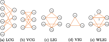
Figure 1: Graph representations of $\Phi_{1}=(x_{1}\lor x_{2}\lor x_{3})\land(x_{1}\lor\neg x_{2}\lor x_{3})\land(\neg x_{1}\lor\neg x_{2}\lor\neg x_{3})$. (a) – (d) correspond to traditional representations appearing in related literature. (e) WLIG is the proposed novel representation, which merely encodes extra edge weights (literal incidence frequency 1 and 2) compared to (c) LIG. Zoom in to a better view.

⬇

113-71 44 0

11422 -17 71 -72 -44 0

where each line corresponds to a clause, and each number within the same line indicates an involved literal index of its original form or negation (with “-” ahead). Such text format can be easily converted to incidence frequency between literals and also inspires us to perform initial feature extraction using Word2Vec (Mikolov et al., 2013), which will be detailed in Section 4.3.

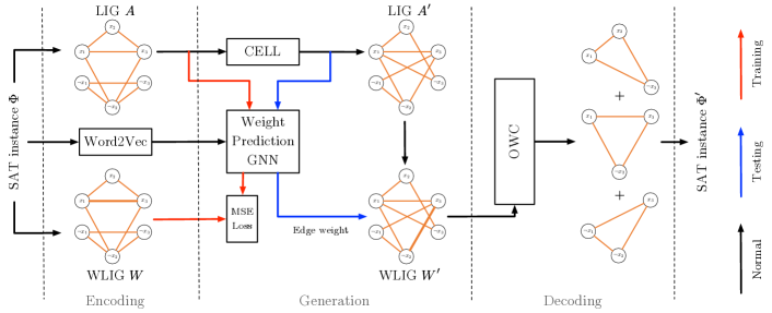
Figure 2: An overview of W2SAT framework. We use RED and BLUE arrowed lines to indicate flows in the training and the testing phases, respectively. Black arrowed lines are normal flows. Zoom in to a better view.

Graph representations of SAT. Traditionally, there are four graph representations to depict a CNF formula in research, including a) Literal-Clause Graph (LCG), b) Variable-Clause Graph (VCG), c) Literal-Incidence Graph (LIG), and d) Variable-Incidence Graph (VIG). The LCG is composed of nodes representing both literals and clauses, with edges indicating the presence of a specific literal within a clause. This graph is bipartite and the mapping between the graph and CNF formula is bijective. The VCG is derived from the LCG by merging a node (literal) and its negation. Nodes in LIG represent individual literals and edges between literals indicate the co-occurrence of two ending nodes in a clause. Similarly, the VIG is obtained by applying the same merging operation in literals on the LIG. In our work, we propose a novel graph representation – WLIG – for encoding a CNF formula. The WLIG extends the LIG, but encodes literals co-occurrence frequency as edge weight in the graph. A more detailed description and analysis of WLIG can be found in Section 4.1. Fig. 1 summarizes the graph representations as mentioned above.

Notations. A weighted graph $\mathcal{G}=(V,E,A,W)$ with $n$ nodes and $m$ edges consists of node set $v_{i}\in V$ for $i=1,...,n$ and edge set $E\subseteq V\times V$ with $|E|=k$. $A\in\{0,1\}^{n\times n}$ and $W\in\mathbb{R}_{+}^{n\times n}$ are the corresponding adjacency matrix and weight matrix, respectively. Throughout our setting, graph $\mathcal{G}$ is undirected such that $A=A^{\top}$ and $W=W^{\top}$. $\mathcal{G}$ may also be associated with node feature $X\in\mathbb{R}^{n\times d}$, where $d$ is the feature dimension. Unless specified, we use $n$ and $m$ to indicate the numbers of literals and clauses of a formula, respectively.

4 W2SAT

In this part, we elaborate on the framework of W2SAT in detail. A high-level overview of the W2SAT framework can be found in Fig. 2. As shown, the framework consists of three core blocks: “Encoding”, “Generation”, and “Decoding”, acting in the presented order. Given an input SAT formula $\Phi$, the Encoding block calculates the corresponding LIG $A$ and WLIG $W$, as well as features of literals output by Word2Vec (Mikolov et al., 2013). In the following generation block, we employ CELL (Rendsburg et al., 2020) to sample a new LIG $A^{\prime}$. In parallel to CELL, we adopt a GCN (Kipf & Welling, 2017) to train a weight predictor taking literal features and $A$ as input, to optimize the MSE error w.r.t. the real incidence frequency in $W$. During the testing phase, the sampled LIG $A^{\prime}$ is instead fed into this predictor as the graph topology, and the new WLIG $W^{\prime}$ is obtained by filling predicted weights into $A^{\prime}$. In the last block of Decoding, OWC performs a hill-climbing strategy to produce the most likely overlapping cliques out of $W^{\prime}$. Finally, this collection of cliques is readily converted to a new SAT instance $\Phi^{\prime}$ in the CNF format. We detail each block in the following sections.

4.1 Encoding – Weighted Literal Incidence Graph

Here we introduce the key concept of the Weighted Literal Incidence Graph (WLIG). WLIG is an extension of LIG, by allowing non-negative weights on edges. These weights carry not only the incidence of literals, but also the frequency of co-occurrence. It is easy to derive that the degree of each node in WLIG corresponds to the total frequency it appears in clauses. We can readily encode a WLIG using a matrix $W\in\mathbb{R}_{+}^{n\times n}$.

On the one hand, we argue that WLIG is a more compact graph representation compared to bipartite-graph-based ones (i.e., LCG and VCG). Note there are $n$ nodes in WLIG corresponding $n$ literals, while in LCG the number of nodes $n+m$ is the sum of literals and clauses. In most of the real-world and industrial SAT instances as in SATLib (Hoos & Stützle, 2000), $m$ is much larger than $n$. Moreover, it is discussed in (Bojchevski et al., 2018; Rendsburg et al., 2020) that bipartite graphs are very hard to be learned with spectral tools, as bitpartite graphs do not have steady states, but WLIG is without such issues. In this sense, WLIG can greatly facilitate modeling and learning SAT instances compared to LCG and VCG. We show more empirical results in Sec. 5.2.

On the other hand, the WLIG is remarkable with higher representation ability than LIG and VIG. For example, SAT-GEN (Wu & Ramanujan, 2019) needs to query back the original SAT instance for clause numbers. After sampling a set of cliques to generate a new formula the initial generation step, SAG-GEN then takes a trivial 1-to-3 equivalent expansion operation by uniformly choosing a clause from the instance until the clause numbers of the generation instance are equal or close to the original one. However, this is unnecessary in W2SAT, as we can decode a new instance solely and directly from a WLIG that highly resembles the characteristics of the original one. Here, we give a proposition about the rationality of WLIGs.

Proposition 1.

One clause of a SAT formula can be mapped to a clique on its LIG and WLIG. All these cliques cover the LIG and the WLIG.

Proof.

By the definition of LIG/WLIG, an edge exists if the two ending nodes/literals co-occur in one clause. Thus each clause has a corresponding clique in LIG/WLIG. Conversely, each pair of ending literals of an edge must be contained in at least one clause, otherwise there will be no corresponding edge. ∎

Though Proposition 1 seems obvious, it motivates us to regard decoding from WLIGs as a clique covering problem, as well as in SAT-GEN (Wu & Ramanujan, 2019).

Input: weighted adjacency matrix $W$, set of cliques $\mathcal{C}$, clause number $m$

Output: set of chosen cliques $\mathtt{Cover}$

1

2function $\mathrm{GenerateEdgeTable}{(}\mathcal{C}{)}$

3      

      $\mathcal{E}\leftarrow\{e_{1}:\varnothing,\cdots,e_{n}:\varnothing\}$ // Edge table

4      

5      forall $e\in\mathcal{E},C\in\mathcal{C}$ do

6             if $e\in C$ then

7                   $\mathcal{E}[e]\leftarrow\mathcal{E}[e]\cup C$

8            

9      

10      return $\mathcal{E}$

11

12function $\mathrm{OWC}{(}W,\mathcal{C},m{)}$

13       $\mathtt{Cover}\leftarrow\varnothing$

       $\mathtt{GT}\leftarrow\{C_{1}:g_{1},\cdots,C_{n}:g_{n}\}$// Gain table

14       $\mathcal{E}\leftarrow\mathrm{GenerateEdgeTable}(\mathcal{C})$

15       for $k\leftarrow 1$ to $m$ do

16             $C^{\prime}\leftarrow\mathrm{LargestGain}(\mathtt{GT})$

17             $\mathtt{Cover}\leftarrow\mathtt{Cover}\cup C^{\prime}$

18             $\mathtt{GT}[C^{\prime}]\leftarrow-\infty$

19             $W\leftarrow\mathrm{Update}(W,C^{\prime})$

20            for $\text{Edge}\ e\in C^{\prime}$ do

21                   $\mathtt{Cliques}\leftarrow\mathcal{E}[e]$

22                   for $C\in\mathtt{Cliques}$ do

23                         $\mathtt{GT}[c]\leftarrow\mathrm{Update}^{\prime}(W,C)$

24                        

25                  

26            

27      

28      return $\mathtt{Cover}$

29

Algorithm 1 Optimal Weight Coverage (OWC)

4.2 Decoding – from WLIGs to formulas

Although SAT formulas can be easily converted into WLIGs, their inversion is non-trivial. Before diving into the details of our problem, we briefly discuss how decoding into SAT is modeled via LIG in SAT-GEN (Wu & Ramanujan, 2019). In SAT-GEN, each clause in the original formula corresponds to one clique in LIG, then recovering a SAT formula from a LIG is modeled as an NP-complete Minimal Clique Edge Cover (MCEC) problem (Karp, 1972): choosing minimal numbers of cliques from the LIG such that their union covers all the edges in the LIG. To tackle this, a greedy hill-climbing algorithm was designed in SAT-GEN (Wu & Ramanujan, 2019). Putting aside the extremely computation-consuming LIG generation procedure (i.e., NetGAN (Bojchevski et al., 2018)), SAT-GEN is still problematic from two aspects: 1) LIG-based modeling significantly limits its representation ability as omitting rich statistics such as literal incidence frequency and degree information; and 2) Solving MCEC using the proposed algorithm in SAT-GEN tends to produce remarkably less number of clauses than the original SAT formula, especially for LIGs with strong connectivity. Though Wu & Ramanujan (2019) devise a procedure randomly breaking down “large” cliques to enlarge the clique number, this strategy maintains the satisfiability of large cliques and may result in an arbitrary change of LIG statistics. To address these issues, derived from WLIG, we raise a novel Weighed Clique Edge Cover (WCEC) problem and an associated efficient algorithm Optimal Weight Coverage (OWC) in a hill-climbing manner.

Weighted Clique Edge Cover Problem (WCEC). Though there exist several variants of clique covering problems, our problem of recovering clique covers from weighted graphs has been less studied. The most related problem in literature is Weighted Edge Clique Partition (WECP), which is proposed by (Feldmann et al., 2020). We modify an approximate version of WECP for our setting:

Problem 1 (Weighted Clique Edge Cover).

Given a weighted graph $\mathcal{G}$ with weight matrix $W$, it asks to select $k$ cliques from $\mathcal{G}$, such that the distance $d(W,W^{\prime})\geq 0$ between $W$ and $W^{\prime}$ is miminized, where weight matrix $W^{\prime}$ is derived from a new weighted graph $\mathcal{G}^{\prime}$ by stacking $k$ selected cliques.

In our setting, we let $d(W,W^{\prime})$ be the L1-distance:

$$d(W,W^{\prime})=\sum_{i=1}^{n}\sum_{j=1}^{n}\lvert W_{ij}-W^{\prime}_{ij}\rvert,$$ (2)

where $W_{ij}$ represents the entry of $W$ at $i$th row and $j$th column. Comparing the proposed WCEC and MCEC in SAT-GEN (Wu & Ramanujan, 2019), we have the following lemma:

Lemma 2.

Suppose a WCEC problem with weight matrix $W$ is obtained by assigning positive weights to edges in adjacency $A$ associated with an MCEC problem. Then a solution clique cover to this WCEC such that $d(W,W^{\prime})=0$ must form a cover of the MCEC, but a clique cover of MCEC on $A$ may not satisfy $d(W,W^{\prime})=0$.

Proof.

We prove the first part. By definition, $d(W,W^{\prime})=0$ indicates for every $(i,j)$, the WLIG weight matrix of the found cover $W^{\prime}_{i,j}=W_{i,j}$. As $W$ is derived by assigning positive weights to non-zero entries in $A$, we must have $W^{\prime}_{i,j}>0\rightarrow A_{i,j}=1$ and $W^{\prime}_{i,j}=0\rightarrow A_{i,j}=0$. Therefore, the solution to the WCEC is a cover of the MCEC. For the second part, it only suffices to raise an example which is easy to prove. ∎

Lemma 2 provides an interpretation of why the proposed framework “WLIG+WCEC” is more powerful than “LIG+MCEC” utilized by (Wu & Ramanujan, 2019). In general, solving WCEC provides rich information for solving MCEC, but not vice versa. Nevertheless, solving either of them is NP-complete (Feldmann et al., 2020; Ullah, 2022).

Optimal Weight Coverage (OWC) Algorithm. Due to the NP-completeness, WCEC has no polynomial-time solution. Therefore, in this section, we develop a specialized algorithm to obtain a local optima of WCEC via hill-climbing. Our algorithm works on a local search basis, in which each iteration will take action with the largest gain. Inspired by the decoding procedure devised in SAT-GEN (Wu & Ramanujan, 2019), we proposed the Optimal Weight Coverage (OWC) algorithm. Concretely, OWC first enumerates all the cliques in a WLIG, whose sizes are below the maximal clause size of the original SAT formula, using (Zhang et al., 2005). Then we create a $\mathtt{GainTable}$ measuring how much one can improve by decoding the corresponding clique. In each of the following steps, OWC finds a clique with the largest gain and updates the $\mathtt{GainTable}$, until the number of found cliques reaches a preset threshold $m$ or distance. To prevent redundant computation, we first build an $\mathtt{EdgeTable}$ mapping from an edge to its related cliques, which allows OWC only updates the gain of the local cliques in each step. Alg. 1 sketches the algorithm. In the implementation, we conduct a series of optimization to accelerate OWC.

Empirically, we find OWC is quite efficient for decoding the WLIGs learned from real-world and industrial SAT instances. Fig. 3 demonstrates the running time of OWC under varying sizes of 17 selected SAT instances. We see “WLIG + OWC” alone is quite efficient. We leave the more theoretical analysis to our future work.

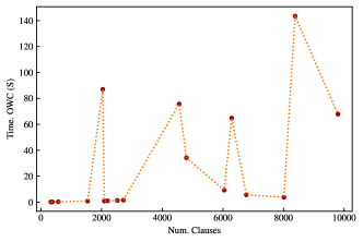
Figure 3: OWC cost for different instances. The cost does not grow monotonically with the clause size, cause the run time of OWC is highly dependent on the structure of the graph.

4.3 Generation – Learn to generate WLIGs

Weighted Graph Generation. Generating WLIGs that resemble a WLIG derived from a real-world SAT instance is non-trivial, as 1) WLIGs with weights are hard to model and learn, and 2) real-world instances can easily scale up (to tens of thousands of literals) with strong global structures. We first present how this can be achieved at a high level. Considering a graph (corresponding to a formula) with node feature $X\in\mathbb{R}^{n\times d}$, adjacency matrix $A$, and weight matrix $W$, we have:

$$\mathbb{P}(W,A|X) =\mathbb{P}(W|A,X)\mathbb{P}(A)$$ (3a)

$$=\mathbb{P}(W|A,X)\prod_{i,j}\mathbb{P}(A_{i,j})$$ (3b)

$$=\prod_{i,j}\mathbb{P}(W_{i,j}|A_{i,j},X)\prod_{i,j}\mathbb{P}(A_{i,j})$$ (3c)

$$=\prod_{i,j}\mathbb{P}_{\alpha}(W_{i,j}|A_{i,j},X_{i},X_{j})\mathbb{P}_{\beta}(A_{i,j}),$$ (3d)

where $\mathbb{P}(\cdot)$ measures the probability. Eq. (3a) stands because $A$ is derived solely from a spectral method, independent of $X$. Eq. (3b) is due to the fact that $A$ is drawn from an edge-independent “score matrix” as in (Bojchevski et al., 2018; Rendsburg et al., 2020). Eq. (3c) and (3d) are further built upon the assumption that edge weight $W_{ij}$ is only dependent on the features of the ending nodes $X_{i}$ and $X_{j}$, and the existence of this edge $A_{i,j}$, under two distributions parameterized by $\alpha$ and $\beta$.

We first introduce $\mathbb{P}_{\beta}(\cdot)$ allowing for generating large-scale graphs with high efficiency. To this end, we employ CELL (Rendsburg et al., 2020). CELL is a graph generative model working in the spectral space by removing redundant computation from NetGAN (Bojchevski et al., 2018). In NetGAN, the following objective is optimized

$$\begin{split}\min_{Z\in\mathbb{R}^{n\times n}}&-\sum_{(u,v)\in\mathcal{R}}\log\sigma_{\text{rows}}(Z)_{u,v},\\ \text{s.t.}\quad&\mathrm{rank}(Z)\leq h\end{split}$$ (4)

where $\mathcal{R}$ is a collection of (massive) random walks and $(u,v)$ is a transition. $\sigma_{\text{rows}}(Z)$ is a row-wise softmax function perform on the low-rank variable $Z$. In practice, NetGAN needs to sample millions of random walks from a graph with moderate size, which is prohibitively expensive. Besides, the extra computational burden is required as NetGAN trained a generator to produce fixed-length random walks to obtain a new graph.

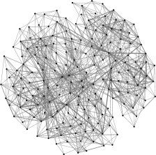
(a) WLIG of ssa2670-141

(b) Generated WLIG via W2SAT

(c) WLIG of decoded formula

Figure 4: Visualization of WLIGs of SAT instance ssa2670-141 at different phases. Each node corresponds to one literal and each edge (with thickness) indicates inter-node incidence (with frequency). (a) WLIG derived from original SAT instance; (b) Generated WLIG based on (a) using our framework; (c) WLIG of decoded instance from (b) with OWC. Zoom in for a better view.

CELL (Rendsburg et al., 2020) argued that such a massive amount of sampling procedures and the generator in NetGAN can be avoided by only considering the spectral properties in limit. Concretely, given the adjacency matrix $A$ of a graph, its transition matrix can be obtained via $P=D^{-1}A$ where $D=\mathrm{diag}(d)\in\mathbb{R}_{+}^{n\times n}$ is the degree matrix. Assuming the stationary state $\pi$ of $P$ exists and is unique, CELL considers acting an infinite number of infinite long random walks and calculates how many times a node can be visited. The time of visit for nodes can be encoded in a “score matrix” $S$, and the normalized score matrix in limit is

$$\lim_{\begin{subarray}{c}q\to\infty\\ T\to\infty\end{subarray}}\frac{S}{qT}=\mathrm{diag}(\pi)P,$$ (5)

where $q$ and $T$ are number and length of random walks, respectively. Thus $S$ can serve as a surrogate of random walk set $\mathcal{R}$ in Eq. (4):

$$\min_{Z\in\mathbb{R}^{n\times n}}-\sum_{u,v=1}^{n}S_{u,v}\log\sigma_{\text{rows}}(Z)_{u,v},$$ (6)

Since $\mathrm{diag}(\pi)P\propto A$ and rescaling $S$ will not change the optima in Eq. (6), the final objective of CELL becomes

$$\begin{split}\min_{Z\in\mathbb{R}^{n\times n}}&-\sum_{u,v=1}^{n}A_{u,v}\log\sigma_{\text{rows}}(Z)_{u,v},\\ \text{s.t.}\quad&\mathrm{rank}(Z)\leq h\end{split}$$ (7)

whose solution is denoted as $Z^{*}$. Then $P^{*}=\sigma_{\text{rows}}(Z^{*})$ can be viewed as a low-rank-regularized transition matrix. We can obtain a new score $S^{*}=\mathrm{diag}(\pi^{*})P^{*}$, where $\pi^{*}$ is the stationary distribution of $P^{*}$. Finally, the edges of a new graph can be independently sampled according to $S^{*}$.

Next, we discuss $\mathbb{P}_{\alpha}(\cdot)$. To allow generating graphs with weights, we extend CELL by providing predicted weights on the sampled edges, where the edge weight predictor is a Graph Convolutional Network (GCN) (Kipf & Welling, 2017). During the training phase, this predictor takes the literal embeddings $X^{(0)}$ and the adjacency matrix $A$ as input, and outputs a set of new embedding $X^{(l)}$:

$$X^{(l)}=\mathrm{GCN}(X^{(0)},A),$$ (8)

where $l$ is the number of basic GCN layers. The loss is the MSE between the predicted weights $X^{(l)}X^{(l)\top}$ and the ground-truth weights $W$ of the original WLIG on the observed edge set $A$:

$$\sum_{(i,j)\in A}\left(\left(X^{(l)}X^{(l)\top}\right)_{i,j}-W_{i,j}\right)^{2}.$$ (9)

This weight predictor can be trained not only on a single SAT formula (though we train separate embedding networks for each instance) but throughout a set of formulas, since all these formulas may share common structures on weights. In the testing stage, we feed the embedding $X^{0}$ and a sampled adjacency $A^{\prime}$ from CELL into the well-trained GCN:

$$X^{(l)}_{s}=\mathrm{GCN}(X^{(0)},A^{\prime}).$$ (10)

Then weights can be derived using $X^{(l)}_{s}X^{(l)\top}_{s}$. We only consider the weights on the edges that appear in $A^{\prime}$. See “Generation” block in Fig. 2 for an intuitive view.

Table 1: Graph statistics on ssa2670-141. Best in bold.

	num clau.	VIG clust.	LIG clust.	VIG mod.	LIG mod.	VCG mod.	LCG mod.
SSa2670-141	377	0.582	0.351	0.521	0.562	0.637	0.587
SAT-GEN	$377.5$	$0.513$	$\mathbf{0.340}$	$0.477$	$0.542$	$\mathbf{0.632}$	$0.537$
PS (T=0)	$273.75$	$0.818$	$0.616$	$0.678$	$0.732$	$0.832$	$\mathbf{0.588}$
PS (T=1.5)	352	$\mathbf{0.572}$	$0.464$	$0.482$	$0.584$	$0.731$	$0.552$
CA	375	$0.368$	$0.247$	$0.412$	$0.499$	$0.629$	$0.502$
W2SAT	377	0.539	0.435	0.520	0.576	0.664	0.527

Literal Embedding. One remaining problem is how to obtain the initial Node Embedding $X^{(0)}$ for each literal. One of the most intuitive ways is to use a one-hot representation, but as the size of the SAT instance grows, the SAT literals number $n$ and the required dimension increase rapidly. NeuroSAT (Selsam et al., 2019) adopts random low-dimension vectors as the initial literal embeddings, but it does not capture the co-occurrence information between the literals in the original SAT formulas. Therefore, here we employ Word2Vec (Mikolov et al., 2013) for computing the initial node embeddings. In our framework, each clause is treated as a sentence, and each literal is treated as a word. By using the Continuous Bag of Words Model (CBOW) and optimizing the objective on the original SAT problem for each literal embedding $X_{i}$:

we can obtain a low-rank representation $X_{i}$ for each literal with contextual co-occurrence information. Then, $X^{(0)}=[X_{1};\cdots;X_{n}]$ will be fed into Eq. (8) as the initial embeddings.

Remark 3.

Training of literal embeddings using Word2Vec is independent of training of the weighted graph generation module. Once the literal embedding module is well trained, we fix it and start to train the generation module.

5 Experiment

5.1 Protocols

Dataset. Following the common practice in (Wu & Ramanujan, 2019; You et al., 2019; Garzón et al., 2022), we evaluate the performance on SATLib (Hoos & Stützle, 2000) and past SAT competitions, which consist of formulas originated from multiple real-world scenarios. We adopt 17 SAT instances in total, on top of 5 and 10 small SAT instances in (Wu & Ramanujan, 2019) and (You et al., 2019), respectively. This greatly enlarges the scope of the testing set, ranging from 82 to 1731 variables and 327 to 9791 clauses.

Baselines. Since W2SAT generates SAT instances in an autoregressive fashion, which is very different from the variants of G2SAT (You et al., 2019; Garzón et al., 2022), we only compare W2SAT with SAT-GEN (Wu & Ramanujan, 2019), CA (Giráldez-Cru & Levy, 2015) and PS (Giráldez-Cru & Levy, 2017).

Task 1: graph statistics. We verify if the graph-level statistics of the original SAT instances can be well preserved via W2SAT. Therefore, we follow the protocols in (Wu & Ramanujan, 2019; You et al., 2019; Garzón et al., 2022) to investigate the average clustering coefficient (Newman, 2001) of LIG and VIG, and the modularity (Newman, 2006) of LIG, VIG, VCG, and LCG.

Task 2: solver performance. We investigate if the generated and the original real-world instances behave similarly in terms of solver performance on a popular SAT solver: Glucose (Audemard & Simon, 2009). To this end, we select six non-trivial SAT instances (costing $\geq$1s for solving) from the dataset and generate 100 instances for each of them. We choose two sensitive parameters variable_decay and clause_decay in Glucose, and perform grid search on {0.75, 0.80, 0.85, 0.90, 0.95} and {0.7, 0.8, 0.9, 0.99, 0.999} (total 25 combinations), respectively. It is to verify if parameter-tuning on generated instances can help improve the performance of the SAT solver on industrial instances.

5.2 Results

Graph statistics. Graph statistics of SAT instance ssa2670-141 can be found in Tab. 1. More results are in Tab. 3 and Tab. 5 (3rd row for each instance) in the appendix. It is seen on all the graph metrics, W2SAT shows stable and superior performance compared to the selected counterparts. In particular, W2SAT outperforms SAT-GEN (on average) in all metrics by a large margin, which in turn demonstrates the stronger representative power of WLIGs over LIGs. Notably, W2SAT and SAT-GEN are parameter-insensitive, so default parameters can achieve superior stability, while PS and CA require intensive parameter tuning.

Representation ability and recoverability. We investigate how much the original statistics can retain after feeding an instance into different consecutive phases of W2SAT. Results are in Tab. 5 in the appendix. We visualize this process using instance ssa2670-141 in Fig. 4. One can readily find that the main structures of WLIGs in the three phases are well preserved.

Efficiency. We study the efficiency of W2SAT in both the training and the testing stages. Tab. 4 in the appendix summarizes the time cost on all 17 real-world SAT instances. In general, both training and testing are significantly efficient. The maximal generation time on an instance with 1731 variables and 9791 clauses is around 12s. Generating such a size of SAT instance in either SAT-GEN (Wu & Ramanujan, 2019) or G2SAT (You et al., 2019; Garzón et al., 2022) is extremely slow.

SAT solver performance. Results are in Tab. 6 in the appendix. In each entry in the format “$x/y$”, $x$ and $y$ stand for the cost of the original SAT problem and the overall cost of the 100 generated instances, respectively. No significant correlation between original and generated instances can be observed. For non-trivial SAT problems, most generated instances via W2SAT are unSAT and much easier (solved in 0.01s by Glucose) than the original one. This also happens to PS, CA, SAT-GEN, and G2SAT (studied in extensive experiments in (Garzón et al., 2022)), due to the fact that such methods tend to produce trivial unSAT instances. Besides, solvers can be very parameter-sensitive for non-trivial industrial SAT problems, and utilizing graph-driven generation for solver-level parameter-tuning can be problematic. Though G2SAT (You et al., 2019) claimed to achieve solver parameter-tuning using generated instances, Garzón et al. (2022) found it works only on limited and selected cases but without broad applicability. Therefore, we believe graph-based SAT generation methods are with very limited capability for helping improve industrial solvers, unless more essential prior about SAT can be incorporated or signals from solvers can be taken into account. We leave these to our future work.

6 Conclusion

In this paper, we studied a novel graph representation – WLIG – for encoding SAT instances, and accordingly developed an efficient and effective framework – W2SAT – to generate industry-level SAT formulas. WLIGs demonstrated strong representation ability compared to existing inexact graph representations while greatly facilitating learning and generating against the exact representation. This is the first work achieving both. Our method performed efficiently and stably compared to previous state-of-the-art methods in terms of graph-based metrics. We also investigated the limitation of using graph-based SAT generation for parameter-tuning of industrial solvers, and proposed the potential directions for making this procedure applicable.

Appendix A More related work

Graph generative model. Generating graphs is the task of producing imitating graphs by learning structural properties from given graphs (Kipf & Welling, 2016; Jin et al., 2018; Bojchevski et al., 2018). This can be achieved via learning node/edge embeddings and injecting appropriate randomness (Kipf & Welling, 2016; Grover et al., 2019; Wang et al., 2019; Dai et al., 2020). However, methods relying on node/edge embeddings typically focus on local structures, especially when the graph is large. While graph spectral theory poses a direction, some works resort to incorporating spectral space into deep models for modeling global characteristics (Martinkus et al., 2022; Bojchevski et al., 2018; Rendsburg et al., 2020). Among them, CELL (Rendsburg et al., 2020) stands out due to its high efficiency and scalability, by peeling off unnecessary operations from (Bojchevski et al., 2018). Another consideration in parallel is to generate graphs with weights (edge features) (Grover et al., 2019; Niu et al., 2020; Kocayusufoglu et al., 2022), which again heavily depends on embeddings. We note, in the case of SAT (and WLIG) where the scale can span drastically and both local and global properties are essential, there is no ready generative model.

Appendix B Implementation details

Throughout all the experiments, W2SAT is running on an Intel Xeon 2.40GHz CPU. The dimension of literal embedding from Word2Vec is 50. The $\mathrm{GCN}$ consists of two layers, with input/output dimensions 50/128 and 128/128, respectively. We employ ADAM as the optimizer for all learning modules (i.e., Word2Vec, $\mathrm{GCN}$, and CELL). For CELL, we set parameter $\mathtt{edge\_overlap\_limit}=0.8$ which controls the overlapping portion of the generated and the original graphs. For more details, one can refer to the supplementary material.

Appendix C Impact of rank value in CELL

(a) $\mathrm{rank}=8$

(b) $\mathrm{rank}=10$

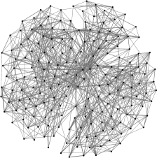
(c) $\mathrm{rank}=12$

Figure 5: Visualization of generated WLIGs of SAT instance ssa2670-141 with different $\mathrm{rank}$ values. Each node corresponds to one literal and each edge (with thickness) indicates inter-node incidence (with frequency). Zoom in for a better view.

Table 2: Graph statistics on different rank in W2SAT of ssa2670-141

	num clau.	VIG clust.	LIG clust.	VIG mod.	LIG mod.	VCG mod.	LCG mod.	steps
SSa2670-141	377	0.582	0.351	0.521	0.562	0.637	0.587
W2SAT(rank=8)	377	0.548	0.461	0.519	0.557	0.651	0.500	240
W2SAT(rank = 10)	377	0.552	0.424	0.516	0.557	0.641	0.501	65
W2SAT(rank = 12)	377	0.539	0.421	0.511	0.554	0.618	0.496	45

The default rank number of CELL (Rendsburg et al., 2020) is 9. To investigate how much this parameter impacts the generated results, we conduct extra experiments on varying $\mathrm{rank}=8,10,12$. Tab. 2 summarizes the graph-based metrics of generated instances of ssa2670-141 on different rank values. We also visualize three generated WLIGs in Fig. 5. Furthermore, in the last column of Tab. 2, we show how many iterations are required under different ranks until convergence. We can conclude that, in terms of graph statistics, there is almost no influence from rank value. However, rank greatly impacts the generation speed in the CELL module. High rank can accelerate the generation greatly but lose some diversity in the generated WLIGs, which is also discussed in (Rendsburg et al., 2020).

Appendix D Results on generating SAT instances

In this section, we present all the remaining results on the selected 17 SAT instances. Among them, there are 5 instances overlapping the setting in SAT-GEN (Wu & Ramanujan, 2019), whose results can be found in Tab. 1 and Tab. 3 for better comparison. As SAT-GEN is not open-sourced and we did not find appropriate parameters for PS and CA as reported in (Wu & Ramanujan, 2019), we only provide the comprehensive graph statistics of W2SAT in Tab. 5 (in the 3rd row of each SAT instance). In general, W2SAT performs stably and efficiency on ALL graph metrics.

Appendix E Results on time cost of different phases of W2SAT

Tab. 4 summarizes the average time cost at different phases in W2SAT. “Time EMB” and “Time CELL” indicate the training cost of the literal embedding networks and the CELL module, respectively. “Time GEN” calculates the OVERALL generation time from one SAT instance $\Phi$ to a new instance $\Phi^{\prime}$. It is seen that W2SAT is far more efficient than other learning-based counterparts (see SAT-GEN (Wu & Ramanujan, 2019) and G2SAT (You et al., 2019) to check the time cost).

Appendix F Results on tuning SAT solvers using generated instances

Results of SAT solver parameter-tuning can be found in Tab. 6. It seems there is no rule or correspondence between the performance on real-world and generated SAT instances. Although You et al. (2019) claimed that SAT solver parameter-tuning could be achieved via G2SAT, a follow-up work (Garzón et al., 2022) with a huge amount of experiments showed it is almost impossible unless instances are carefully selected and manipulated. At the current stage, we suppose that graph-based SAT instance generation alone cannot guarantee good behavior for industrial SAT solvers.

Table 3: Results of SAT instance generation in terms of graph metrics with 4 real-world instances from SATLib.

	num vars.	num clau.	VIG clust.	LIG clust.	VIG mod.	LIG mod.	VCG mod.	LCG mod.
mrpp4_4#4_5	309	2517	0.428	0.357	0.469	0.538	0.784	0.719
SAT-GEN	309	2517.45	0.397	0.331	0.433	0.524	0.695	0.607
PS	309	2361.45	0.658	0.579	0.439	0.526	0.755	0.592
CA	309	2515.50	0.234	0.120	0.401	0.454	0.601	0.525
W2SAT	309	2517	0.429	0.356	0.458	0.543	0.718	0.558
bf0432-007	473	2038	0.493	0.327	0.660	0.783	0.768	0.762
SAT-GEN	473	2038.6	0.417	0.342	0.604	0.772	0.758	0.674
PS	473	1887.5	0.562	0.467	0.718	0.776	0.860	0.624
CA	473	2036.5	0.249	0.177	0.614	0.649	0.746	0.561
W2SAT	473	2038	0.514	0.460	0.672	0.826	0.800	0.638
bmc-ibm-7	860	4797	0.609	0.341	0.716	0.717	0.787	0.719
SAT-GEN	860	4797.4	0.470	0.321	0.671	0.707	0.754	0.649
PS	860	4324.5	0.636	0.535	0.646	0.718	0.858	0.633
CA	860	4796.6	0.185	0.119	0.700	0.711	0.762	0.610
W2SAT	860	4797	0.543	0.448	0.705	0.728	0.767	0.609
countbitsrotate016	1122	4555	0.469	0.421	0.695	0.684	0.801	0.691
SAT-GEN	1122	4555.564	0.302	0.272	0.563	0.618	0.736	0.607
PS	1122	4276.5	0.504	0.426	0.832	0.869	0.912	0.663
CA	1122	4554.5	0.167	0.154	0.668	0.683	0.768	0.543
W2SAT	1122	4555	0.426	0.397	0.620	0.669	0.768	0.601

Table 4: Time cost for each instance in Training and Testing phases

	num vars.	num clau.	Training(s)		Testing(s)
			time EMB	time CELL	time Gen (avg)
ssa2670-130	82	327	50.595	12.702	1.566
ssa2670-141	91	377	57.126	11.750	1.726
mrpp_4x4#4_4	208	1538	164.244	36.288	2.715
mrpp_4x4#4_5	309	2517	182.468	53.209	4.968
mrpp_4x4#6_5	330	2721	186.818	40.931	5.425
mrpp_4x4#8_8	717	6773	262.625	111.062	11.754
countbitssrl016	1691	8378	121.368	115.004	8.521
countbitsrotate016	1122	4555	133.784	86.222	9.817
bmc-ibm-2	119	573	58.833	8.009	1.788
bmc-ibm-5	1068	6042	208.807	124.498	9.071
bmc-ibm-7	860	4797	135.057	120.668	7.042
aes_32_3_keyfind_2	450	2204	187.770	40.327	3.593
aes_64_1_keyfind_1	320	2088	167.153	71.303	3.414
bf0432-007	473	2038	77.084	30.251	3.048
smulo016	1459	6288	164.932	151.759	7.389
sat_prob_83	1759	8012	322.410	102.804	11.534
cmu-bmc-longmult15	1731	9791	232.948	146.801	12.505

Table 5: Results of the graph metrics for original formulas, decode from original formulas and decode from generation formulas

	num vars.	num clau.	VIG clust.	LIG clust.	VIG mod.	LIG mod.	VCG mod.	LCG mod.
ssa2670-130	82	327	0.595	0.375	0.504	0.509	0.630	0.577
(decode from origin)	82	327	0.603	0.451	0.501	0.537	0.645	0.493
(decode from generation)	82	327	0.542	0.482	0.494	0.550	0.619	0.500
ssa2670-141	91	377	0.582	0.351	0.521	0.562	0.637	0.587
	91	377	0.609	0.434	0.546	0.583	0.647	0.508
	91	377	0.539	0.435	0.520	0.576	0.664	0.527
mrpp_4x4#4_4	208	1538	0.448	0.389	0.476	0.561	0.775	0.695
	208	1538	0.448	0.389	0.464	0.541	0.739	0.577
	208	1538	0.457	0.411	0.498	0.552	0.708	0.548
mrpp_4x4#4_5	309	2517	0.428	0.357	0.469	0.538	0.784	0.719
	309	2517	0.427	0.359	0.472	0.553	0.754	0.603
	309	2517	0.429	0.356	0.458	0.543	0.718	0.558
mrpp_4x4#6_5	330	2721	0.426	0.349	0.485	0.518	0.783	0.717
	330	2721	0.428	0.356	0.453	0.505	0.739	0.593
	330	2721	0.431	0.365	0.479	0.528	0.709	0.559
mrpp_4x4#8_8	717	6773	0.395	0.310	0.547	0.567	0.798	0.742
	717	6773	0.398	0.321	0.537	0.577	0.773	0.635
	717	6773	0.398	0.339	0.552	0.590	0.732	0.597
countbitssrl016	1691	8378	0.540	0.435	0.801	0.749	0.816	0.726
	1691	8378	0.540	0.435	0.795	0.758	0.810	0.569
	1691	8378	0.493	0.396	0.767	0.767	0.818	0.573
countbitsrotate016	1122	4555	0.469	0.421	0.695	0.684	0.801	0.691
	1122	4555	0.469	0.421	0.688	0.681	0.781	0.612
	1122	4555	0.426	0.397	0.620	0.669	0.768	0.601
bmc-ibm-2	119	573	0.627	0.357	0.617	0.625	0.661	0.651
	119	573	0.646	0.455	0.613	0.631	0.644	0.537
	119	573	0.597	0.496	0.599	0.631	0.618	0.505
bmc-ibm-5	1068	6042	0.584	0.318	0.762	0.777	0.821	0.752
	1068	6042	0.584	0.384	0.760	0.778	0.820	0.613
	1068	6042	0.506	0.395	0.754	0.777	0.834	0.607
bmc-ibm-7	860	4797	0.609	0.341	0.716	0.717	0.787	0.719
	860	4797	0.612	0.423	0.722	0.732	0.774	0.583
	860	4797	0.543	0.448	0.705	0.728	0.767	0.609
aes_32_3_keyfind_2	450	2204	0.441	0.357	0.693	0.664	0.757	0.657
	450	2204	0.598	0.469	0.745	0.717	0.803	0.580
	450	2204	0.434	0.372	0.675	0.700	0.785	0.580
aes_64_1_keyfind_1	320	2088	0.457	0.393	0.655	0.661	0.754	0.672
	320	2088	0.789	0.654	0.789	0.782	0.820	0.666
	320	2088	0.551	0.437	0.710	0.714	0.765	0.587
bf0432-007	473	2038	0.493	0.327	0.660	0.783	0.768	0.762
	473	2038	0.567	0.438	0.682	0.833	0.792	0.674
	473	2038	0.514	0.460	0.672	0.826	0.800	0.638
smulo016	1459	6288	0.494	0.432	0.685	0.667	0.789	0.721
	1459	6288	0.494	0.432	0.681	0.670	0.776	0.601
	1459	6288	0.442	0.382	0.623	0.654	0.761	0.584
sat_prob_83	1759	8012	0.441	0.388	0.760	0.796	0.871	0.757
	1759	8012	0.505	0.440	0.773	0.812	0.893	0.717
	1759	8012	0.497	0.423	0.739	0.810	0.887	0.671
cmu-bmc-longmult15	1731	9791	0.537	0.400	0.755	0.733	0.779	0.709
	1731	9791	0.541	0.434	0.749	0.740	0.803	0.591
	1731	9791	0.511	0.410	0.732	0.733	0.801	0.606

Table 6: Solver performance. In each entry in the format “$x/y$”, $x$ and $y$ stand for the cost of the original SAT problem and the overall cost of the 100 generated instances, respectively. Best performance among all combinations of parameters is in bold.

vars_decay	clau_decay	countbitssrl016	smulo016	cmu-bmc-longmult15	countbitsrotate016	aes_32_3_keyfind_2	sat_prob_83
0.75	0.7	2.457/0.970	7.878/0.841	12.667/1.213	26.485/0.658	5239.189/0.503	6943.854/0.984
0.75	0.8	2.61/0.984	6.346/0.783	14.913/1.204	21.151/0.657	6136.231/0.490	5372.453/1.020
0.75	0.9	1.961/0.946	6.77/0.843	11.442/1.190	28.091/0.699	3797.059/0.505	3321.887/1.050
0.75	0.99	2.159/0.969	7.499/0.857	12.435/1.263	29.6/0.706	1344.593/0.495	2850.1/1.054
0.75	0.999	1.61/1.002	6.453/0.822	14.63/1.324	30.678/0.708	5473.334/0.565	3334.674/1.031
0.8	0.7	3.277/0.981	6.268/0.816	12.576/1.228	27.387/0.690	2292.523/0.556	5338.714/1.012
0.8	0.8	2.096/0.964	8.721/0.823	15.576/1.240	23.086/0.711	134.786/0.504	6534.409/0.967
0.8	0.9	1.403/1.037	7.304/0.836	11.748/1.156	23.407/0.742	9674.478/0.542	4711.479/1.069
0.8	0.99	2.061/1.020	6.468/0.819	14.301/1.183	22.361/0.686	9748.891/0.502	3735.033/1.104
0.8	0.999	2.399/1.019	5.686/0.717	13.287/1.153	23.745/0.678	8231.243/0.516	3462.053/1.086
0.85	0.7	3.748/0.876	8.324/0.839	10.892/1.271	17.097/0.684	13008.53/0.504	6974.845/1.053
0.85	0.8	2.03/0.995	5.049/0.831	13.091/1.195	22.228/0.627	7992.41/0.498	7343.939/1.018
0.85	0.9	2.771/0.968	5.576/0.828	13.064/1.235	22.645/0.692	10370.113/0.531	4662.903/1.061
0.85	0.99	3.102/0.931	3.768/0.794	11.058/1.230	21.567/0.712	9489.071/0.515	2772.389/1.068
0.85	0.999	4.362/0.999	7.293/0.869	14.54/1.217	22.881/0.640	4815.33/0.474	2016.212/1.074
0.9	0.7	2.016/0.925	4.501/0.812	10.19/1.221	15.288/0.697	56601.926/0.488	5753.988/1.018
0.9	0.8	3.151/0.993	7.059/0.874	12.292/1.204	18.776/0.666	12468.458/0.533	5585.339/1.026
0.9	0.9	3.091/0.907	5.953/0.808	10.318/1.164	17.391/0.663	875.98/0.514	4389.603/0.973
0.9	0.99	2.481/0.967	5.735/0.777	11.986/1.154	15.964/0.772	35765.854/0.612	3232.317/0.991
0.9	0.999	3.464/0.943	6.945/0.807	10.914/1.206	18.078/0.639	5090.965/0.547	2349.351/1.116
0.95	0.7	1.599/0.932	8.417/0.885	8.805/1.199	11.559/0.724	8356.976/0.502	5694.292/0.865
0.95	0.8	2.889/0.966	6.531/0.809	10.4/1.182	11.921/0.664	314.555/0.510	4796.449/1.058
0.95	0.9	3.047/1.082	6.875/0.815	7.33/1.143	12.247/0.720	27458.417/0.507	3004.014/1.070
0.95	0.99	1.898/0.899	4.898/0.836	10.095/1.176	16.513/0.746	461.125/0.489	2649.442/1.006
0.95	0.999	2.34/1.017	6.48/0.863	13.842/1.265	16.94/0.697	3685.33/0.527	2644.514/0.977

References

- Aloul et al. (2003) Aloul, F. A., Ramani, A., Markov, I. L., and Sakallah, K. A. Solving difficult instances of boolean satisfiability in the presence of symmetry. IEEE Transactions on Computer-Aided Design of Integrated Circuits and Systems, 22(9):1117–1137, 2003.
- Ansótegui et al. (2017) Ansótegui, C., Bonet, M. L., Giráldez-Cru, J., and Levy, J. Structure features for sat instances classification. Journal of Applied Logic, 23:27–39, 2017.
- Ansótegui et al. (2022) Ansótegui, C., Bonet, M. L., and Levy, J. Scale-free random sat instances. Algorithms, 15(6):219, 2022.
- Audemard & Simon (2009) Audemard, G. and Simon, L. Predicting learnt clauses quality in modern sat solvers. In Twenty-first international joint conference on artificial intelligence, 2009.
- Bojchevski et al. (2018) Bojchevski, A., Shchur, O., Zügner, D., and Günnemann, S. Netgan: Generating graphs via random walks. In ICML, 2018.
- Braunstein et al. (2005) Braunstein, A., Mézard, M., and Zecchina, R. Survey propagation: An algorithm for satisfiability. Random Structures & Algorithms, 27(2):201–226, 2005.
- Cai & Su (2013) Cai, S. and Su, K. Local search for boolean satisfiability with configuration checking and subscore. Artificial Intelligence, 204:75–98, 2013.
- Clarke et al. (2001) Clarke, E., Biere, A., Raimi, R., and Zhu, Y. Bounded model checking using satisfiability solving. Formal methods in system design, 19(1):7–34, 2001.
- Cook (1971) Cook, S. A. The complexity of theorem-proving procedures. In Proceedings of the third annual ACM symposium on Theory of computing, pp. 151–158, 1971.
- Dai et al. (2020) Dai, H., Nazi, A., Li, Y., Dai, B., and Schuurmans, D. Scalable deep generative modeling for sparse graphs. In ICML, 2020.
- Feldmann et al. (2020) Feldmann, A. E., Issac, D., and Rai, A. Fixed-parameter tractability of the weighted edge clique partition problem. In 15th International Symposium on Parameterized and Exact Computation, 2020.
- Ganzinger et al. (2004) Ganzinger, H., Hagen, G., Nieuwenhuis, R., Oliveras, A., and Tinelli, C. Dpll (t): Fast decision procedures. In International Conference on Computer Aided Verification, pp. 175–188. Springer, 2004.
- Garzón et al. (2022) Garzón, I., Mesejo, P., and Giráldez-Cru, J. On the performance of deep generative models of realistic sat instances. In 25th International Conference on Theory and Applications of Satisfiability Testing (SAT 2022). Schloss Dagstuhl-Leibniz-Zentrum für Informatik, 2022.
- Giráldez-Cru & Levy (2015) Giráldez-Cru, J. and Levy, J. A modularity-based random sat instances generator. In Twenty-Fourth International Joint Conference on Artificial Intelligence, 2015.
- Giráldez-Cru & Levy (2017) Giráldez-Cru, J. and Levy, J. Locality in random sat instances. In International Joint Conferences on Artificial Intelligence, 2017.
- Giráldez-Cru & Levy (2021) Giráldez-Cru, J. and Levy, J. Popularity-similarity random sat formulas. Artificial Intelligence, 299:103537, 2021.
- Grover et al. (2019) Grover, A., Zweig, A., and Ermon, S. Graphite: Iterative generative modeling of graphs. In ICML, 2019.
- Guo et al. (2022) Guo, W., Yan, J., Zhen, H.-L., Li, X., Yuan, M., and Jin, Y. Machine learning methods in solving the boolean satisfiability problem. arXiv preprint arXiv:2203.04755, 2022.
- Hoos & Stützle (2000) Hoos, H. H. and Stützle, T. Satlib: An online resource for research on sat. Sat, 2000:283–292, 2000.
- Jin et al. (2018) Jin, W., Barzilay, R., and Jaakkola, T. Junction tree variational autoencoder for molecular graph generation. In ICML, 2018.
- Karp (1972) Karp, R. M. Reducibility among combinatorial problems. In Complexity of computer computations, pp. 85–103. Springer, 1972.
- Kautz et al. (1992) Kautz, H. A., Selman, B., et al. Planning as satisfiability. In ECAI, volume 92, pp. 359–363, 1992.
- Kipf & Welling (2016) Kipf, T. N. and Welling, M. Variational graph auto-encoders. arXiv preprint arXiv:1611.07308, 2016.
- Kipf & Welling (2017) Kipf, T. N. and Welling, M. Semi-supervised classification with graph convolutional networks. In ICLR, 2017.
- Kocayusufoglu et al. (2022) Kocayusufoglu, F., Silva, A., and Singh, A. K. Flowgen: A generative model for flow graphs. In Proceedings of the 28th ACM SIGKDD Conference on Knowledge Discovery and Data Mining, 2022.
- Liang et al. (2016) Liang, J., Ganesh, V., Poupart, P., and Czarnecki, K. Exponential recency weighted average branching heuristic for sat solvers. In AAAI, 2016.
- Liang et al. (2017) Liang, J. H., VK, H. G., Poupart, P., Czarnecki, K., and Ganesh, V. An empirical study of branching heuristics through the lens of global learning rate. In International conference on theory and applications of satisfiability testing, pp. 119–135, 2017.
- Luo et al. (2017) Luo, M., Li, C.-M., Xiao, F., Manya, F., and Lü, Z. An effective learnt clause minimization approach for cdcl sat solvers. In Proceedings of the 26th International Joint Conference on Artificial Intelligence, pp. 703–711, 2017.
- Marques-Silva et al. (2021) Marques-Silva, J., Lynce, I., and Malik, S. Conflict-driven clause learning sat solvers. In Handbook of satisfiability, pp. 133–182. IOS Press, 2021.
- Marques-Silva & Sakallah (2000) Marques-Silva, J. P. and Sakallah, K. A. Boolean satisfiability in electronic design automation. In Proceedings of the 37th Annual Design Automation Conference, pp. 675–680, 2000.
- Martinkus et al. (2022) Martinkus, K., Loukas, A., Perraudin, N., and Wattenhofer, R. Spectre: Spectral conditioning helps to overcome the expressivity limits of one-shot graph generators. In ICML, 2022.
- Mikolov et al. (2013) Mikolov, T., Chen, K., Corrado, G., and Dean, J. Efficient estimation of word representations in vector space. arXiv preprint arXiv:1301.3781, 2013.
- Newman (2001) Newman, M. E. Clustering and preferential attachment in growing networks. Physical review E, 64(2):025102, 2001.
- Newman (2006) Newman, M. E. Modularity and community structure in networks. Proceedings of the national academy of sciences, 103(23):8577–8582, 2006.
- Niu et al. (2020) Niu, C., Song, Y., Song, J., Zhao, S., Grover, A., and Ermon, S. Permutation invariant graph generation via score-based generative modeling. In International Conference on Artificial Intelligence and Statistics, 2020.
- Rendsburg et al. (2020) Rendsburg, L., Heidrich, H., and Von Luxburg, U. Netgan without gan: From random walks to low-rank approximations. In ICML, 2020.
- Selman et al. (1993) Selman, B., Kautz, H. A., Cohen, B., et al. Local search strategies for satisfiability testing. Cliques, coloring, and satisfiability, 26:521–532, 1993.
- Selsam et al. (2019) Selsam, D., Lamm, M., Bünz, B., Liang, P., de Moura, L., and Dill, D. L. Learning a SAT solver from single-bit supervision. In ICLR, 2019.
- Ullah (2022) Ullah, A. Computing clique cover with structural parameterization. arXiv preprint arXiv:2208.12438, 2022.
- Wang et al. (2019) Wang, H., Wang, J., Wang, J., Zhao, M., Zhang, W., Zhang, F., Li, W., Xie, X., and Guo, M. Learning graph representation with generative adversarial nets. IEEE Transactions on Knowledge and Data Engineering, 33(8):3090–3103, 2019.
- Wu & Ramanujan (2019) Wu, H. and Ramanujan, R. Learning to generate industrial sat instances. In Twelfth Annual Symposium on Combinatorial Search, 2019.
- Xu et al. (2012) Xu, L., Hutter, F., Shen, J., Hoos, H. H., and Leyton-Brown, K. Satzilla2012: Improved algorithm selection based on cost-sensitive classification models. Proceedings of SAT Challenge, pp. 57–58, 2012.
- You et al. (2019) You, J., Wu, H., Barrett, C., Ramanujan, R., and Leskovec, J. G2sat: Learning to generate sat formulas. NeurIPS, 2019.
- Zhang et al. (2005) Zhang, Y., Abu-Khzam, F. N., Baldwin, N. E., Chesler, E. J., Langston, M. A., and Samatova, N. F. Genome-scale computational approaches to memory-intensive applications in systems biology. In SC’05: Proceedings of the 2005 ACM/IEEE Conference on Supercomputing, pp. 12–12. IEEE, 2005.