Kpc-scale properties of dust temperature in terms of dust mass and star formation activity

Abstract

We investigate how the dust temperature is affected by local environmental quantities, especially dust surface density ($\Sigma_{\mathrm{dust}}$), dust-to-gas ratio (D/G) and interstellar radiation field. We compile multi-wavelength observations in 46 nearby galaxies, uniformly processed with a common physical resolution of 2 kpc. A physical dust model is used to fit the infrared dust emission spectral energy distribution (SED) observed with WISE and Herschel. The star formation rate (SFR) is traced with GALEX ultraviolet data corrected by WISE infrared. We find that the dust temperature correlates well with the SFR surface density ($\Sigma_{\rm SFR}$), which traces the radiation from young stars. The dust temperature decreases with increasing D/G at fixed $\Sigma_{\rm SFR}$ as expected from stronger dust shielding at high D/G, when $\Sigma_{\mathrm{SFR}}$ is higher than $\sim 2\times 10^{-3}~{}\rm M_{\odot}~{}yr^{-1}~{}kpc^{-2}$. These measurements are in good agreement with the dust temperature predicted by our proposed analytical model. Below this range of $\Sigma_{\mathrm{SFR}}$, the observed dust temperature is higher than the model prediction and is only weakly dependent on D/G, which is possibly due to the dust heating from old stellar population or the variation of SFR within the past $10^{10}$ yr. Overall, the dust temperature as a function of $\Sigma_{\mathrm{SFR}}$ and $\Sigma_{\mathrm{dust}}$ predicted by our analytical model is consistent with observations. We also notice that at fixed gas surface density, $\Sigma_{\rm SFR}$ tends to increase with D/G, i.e. we can empirically modify the Kennicutt-Schmidt law with a dependence on D/G to better match observations.

1 Introduction

Dust is a key component in the interstellar medium (ISM). In the diffuse ISM of the Milky Way (MW), roughly 20–50 per cent of metals reside in solid dust grains according to elemental depletions ($F_{*}=0$ to 1 in Jenkins, 2009). Dust grains absorb and scatter a significant fraction of starlight in galaxies (e.g. 30 per cent suggested in Bernstein et al., 2002), and re-radiates the absorbed energy in the infrared (IR, Calzetti, 2001; Buat et al., 2012). These processes regulate the spectral energy distribution (SED) of the interstellar radiation field (ISRF). Dust catalyzes the formation of H₂ (Gould & Salpeter, 1963; Draine, 2003; Cazaux & Tielens, 2004; Yamasawa et al., 2011; Galliano et al., 2018), which helps the formation of the molecular phase ISM. Because of the major roles of dust in galaxy evolution and chemistry, it is important to track the interaction between dust and the ISRF in various environments in the ISM. In particular, the dust surface density is of critical importance because it is not only an indicator of the dust mass but also is proportional to the dust optical depth.

The dust surface density ($\Sigma_{\mathrm{dust}}$) in the ISM can be obtained by analyzing the dust emission SED in the IR (Desert et al., 1990; Draine & Li, 2007; Compiègne et al., 2011; Jones et al., 2017; Relaño et al., 2020; Hensley & Draine, 2022). The intensity of dust emission is proportional to the dust mass at fixed wavelength and is a monotonically increasing function of the dust temperature. The dust temperature (${T_{\mathrm{dust}}}$), or the radiation field heating up dust in some models, can be constrained with the ratio between dust emission at different photometric bands in the measured SED. With the obtained value for ${T_{\mathrm{dust}}}$, we are able to derive $\Sigma_{\mathrm{dust}}$ from the intensity of dust emission with an assumption of grain emissivity.

With multi-band far-IR (FIR) data, especially the 70–500 µm photometry obtained with the Herschel Space Observatory (Pilbratt et al., 2010), there have been many efforts to measure spatially resolved, emission-based $\Sigma_{\mathrm{dust}}$ and ${T_{\mathrm{dust}}}$ in nearby galaxies (e.g. Aniano et al., 2012; Bendo et al., 2012; Smith et al., 2012; Draine et al., 2014; Gordon et al., 2014; Tabatabaei et al., 2014; Bendo et al., 2015; Davies et al., 2017; Bianchi et al., 2018; Utomo et al., 2019; Vílchez et al., 2019; Aniano et al., 2020; Chiang et al., 2021; Nersesian et al., 2021). Meanwhile, observations of distant (high-redshift) galaxies are often performed with the Atacama Large Millimeter/submillimeter Array (ALMA) because of increased requirements for spatial resolution and sensitivity (e.g. Capak et al., 2015; Watson et al., 2015; Bouwens et al., 2016; Liu et al., 2019). Due to the narrow instantaneous frequency coverage of ALMA, each galaxy is observed in a limited number of wavelength bands, usually only 1–2 bands, and as a result the dust temperatures in these systems remain comparatively uncertain. In spite of these limitations, the observed dust temperatures by ALMA have provided meaningful insight into the physical conditions in the ISM at high redshift. Studies that succeeded in obtaining multi-band ALMA data suggested that high-redshift ${T_{\mathrm{dust}}}$ spans $\sim$30–70 K (see the $z$$\sim$5–8.3 data compiled in Burgarella et al., 2020; Bakx et al., 2021), which is not only warmer but also showing a larger variety than the dust temperatures observed in nearby disc galaxies, e.g. $\sim$17–40 K in the KINGFISH samples (Dale et al., 2012) and $\sim$15–25 K in the Local Group (Utomo et al., 2019). High dust temperatures in distant galaxies are also indicated by some indirect estimates using the ultraviolet (UV) optical depth or the [C ii] 158 µm line (Sommovigo et al., 2022; Ferrara et al., 2022). These results indicate that the ISRFs are high probably because of intense star formation activity in high-redshift galaxies.

In Hirashita & Chiang (2022, hereafter Paper I), we built analytical models that evaluate how dust temperature varies with relevant physical quantities, i.e. dust surface density and ISRF, to clarify the physical conditions that possibly cause the observed high and scattered ${T_{\mathrm{dust}}}$ in high-redshift galaxies. With these models, we predicted that to the first order, ${T_{\mathrm{dust}}}$ increases with UV radiation from stars (traced by the star formation rate surface density, $\Sigma_{\mathrm{SFR}}$). This supports the above-mentioned view of intense star formation activity in high-redshift galaxies. We also found that, at fixed $\Sigma_{\mathrm{SFR}}$, dust temperature increases towards lower dust-to-gas ratio (D/G). This is because of less shielding of ISRF by dust (see also Sommovigo et al., 2022). Moreover, with $\Sigma_{\mathrm{SFR}}$ and $\Sigma_{\mathrm{dust}}$ measured, we can roughly predict the dust temperature, which offers a way to improve the dust mass and temperature estimation iteratively. We tested these predictions against several high-redshift observations.

Although we obtained useful insights using our model, the large uncertainties and low spatial resolutions of high-redshift observations hampered rigid conclusions. Observations with greater precision and larger sample size are useful to validate our dust temperature model in Paper I. For this purpose, observations in the nearby galaxies are suitable in terms of both precision and sample size, as demonstrated by the multi-wavelength datasets in the literature (e.g. Barrera-Ballesteros et al., 2016; Barrera-Ballesteros et al., 2021; Casasola et al., 2017, 2022; Leroy et al., 2019; Enia et al., 2020; Morselli et al., 2020; Ellison et al., 2021; Sánchez et al., 2021; Abdurro’uf et al., 2022a; Sun et al., 2022). These observations also provide measurements at the low $\Sigma_{\mathrm{SFR}}$ and $\Sigma_{\mathrm{dust}}$ end, which was not tested in Paper I. With the availability of multi-band FIR photometric data, e.g. observations made with Herschel, and gas surface densities from high sensitivity emission line observations, e.g. The H i Nearby Galaxy Survey (THINGS) (Walter et al., 2008), The HERA CO-Line Extragalactic Survey (HERACLES) (Leroy et al., 2009) and the ALMA, VLA and MeerKAT surveys conducted in the Physics at High Angular resolution in Nearby Galaxies (PHANGS) project (Leroy et al., 2021b; Sun et al., 2022), we are able to derive dust temperature and D/G more robustly for nearby galaxies.

In this work, we compare our model to a sample of nearby galaxies to investigate what regulates the dust temperature. We compile spatially resolved, multi-wavelength data for 46 nearby galaxies. We uniformly process them with a 2 kpc resolution. We derive key quantities that affect the dust temperature with the following methods: $\Sigma_{\mathrm{dust}}$ is derived from the dust emission SED observed with the Wide-field Infrared Survey Explorer (WISE, Wright et al., 2010) and Herschel using the Draine & Li (2007) physical dust model including the correction factor introduced by Chastenet et al. (2021). We utilize the Galaxy Evolution Explorer (GALEX, Martin et al., 2005) UV data, supplemented by WISE IR, to trace star formation rate (SFR) following the Leroy et al. (2019) prescription. Besides dust temperature, we also examine the scaling relations among the surface densities of dust, SFR and gas, which are necessary to setup the Paper I model. These measurements and comparisons allow us to test the model in Paper I and to clarify how key physical properties, especially star formation activity and dust surface density, regulate the dust temperature.

This paper is organized as follows. In Section 2, we introduce the sample galaxies and data sets used in this work. In Section 3, we describe how we uniformly process the multi-wavelength observations and convert them to desired physical quantities. We also outline how we adapt the Paper I model in this work. We present our measured dust temperature and relevant scaling relations in Section 4. We compare our measurements to the Paper I model and provide some extended discussions in Section 5. Finally, we summarize our key findings in Section 6.

2 Sample and Data

The data necessary for this study are dust surface densities and temperatures from IR photometry, gas surface densities from CO and H i emission lines and SFRs from UV and IR photometry. We select our sample galaxies from the $z=0$ Multiwavelength Galaxy Synthesis ($z$0MGS) catalog (Leroy et al., 2019, J. Chastenet et al. in preparation). We pick the galaxies with Herschel IR, WISE IR and GALEX UV data available as the master sample. From this large sample, we pick 49 galaxies with both low-$J$ CO rotational lines and H i data from archival or our new data. We set the desired physical resolution at 2 kpc, which puts a limitation on distance at $D\lesssim 20~{}\mathrm{Mpc}$, corresponding to $\sim$2 kpc resolution of the coarsest resolution data obtained by the Herschel SPIRE 250 $\micron$ band. Finally, we exclude high-inclination ($>80^{\circ}$) galaxies, which yields 46 galaxies in the end. We list the properties and data sources of these galaxies in Table 1.

Table 1: Sample galaxies.

Galaxy	Dist.	$i$	P.A.	$R_{25}$	$R_{\mathrm{eff}}$	$\log(M_{\star})$	Type	CO Ref	H i Ref	12+log(O/H) Ref
	[Mpc]	[∘]	[∘]	[kpc]	[kpc]	[M⊙]
(1)	(2)	(3)	(4)	(5)	(6)	(7)	(8)	(9)	(10)	(11)
IC0342	3.4	31.0	42.0	9.9	4.3	10.2	5	$a.$	$h.$	$p.$
NGC0224	0.8	77.7	38.0	21.2	–	–	3	$b.$	$i.$	$r.$
NGC0253	3.7	75.0	52.5	14.4	4.7	10.5	5	$c.$	$j.$	–
NGC0300	2.1	39.8	114.3	5.9	2.0	9.3	6	$c.$	$j.$	$r.$
NGC0337	19.5	51.0	90.0	8.3	2.4	9.7	6	$d.$	$k.$	–
NGC0598	0.9	55.0	201.0	8.5	2.5	9.4	5	$e.$	$l.$	$r.$
NGC0628	9.8	8.9	20.7	14.1	3.9	10.2	5	$c.$	$m.$	$q.$
NGC0925	9.2	66.0	287.0	14.3	4.5	9.8	6	$d.$	$m.$	$r.$
NGC2403	3.2	63.0	124.0	9.3	2.4	9.6	5	$d.$	$m.$	$r.$
NGC2841	14.1	74.0	153.0	14.2	5.4	10.9	3	$d.$	$m.$	–
NGC2976	3.6	65.0	335.0	3.0	1.3	9.1	5	$d.$	$m.$	–
NGC3184	12.6	16.0	179.0	13.5	5.3	10.3	5	$d.$	$m.$	$r.$
NGC3198	13.8	72.0	215.0	13.0	5.0	10.0	5	$d.$	$m.$	–
NGC3351	10.0	45.1	193.2	10.5	3.0	10.3	3	$c.$	$m.$	$q.$
NGC3521	13.2	68.8	343.0	16.0	3.9	11.0	3	$c.$	$m.$	–
NGC3596	11.3	25.1	78.4	6.0	1.6	9.5	5	$c.$	$n.$	–
NGC3621	7.1	65.8	343.8	9.8	2.7	10.0	6	$c.$	$m.$	$r.$
NGC3627	11.3	57.3	173.1	16.9	3.6	10.7	3	$c.$	$m.$	$q.$
NGC3631	18.0	32.4	-65.6	9.7	2.9	10.2	5	$f.$	$h.$	–
NGC3938	17.1	14.0	195.0	13.4	3.7	10.3	5	$d.$	$k.$	–
NGC3953	17.1	61.5	12.5	15.2	5.3	10.6	4	$f.$	$h.$	–
NGC4030	19.0	27.4	28.7	10.5	2.1	10.6	4	$f.$	$h.$	–
NGC4051	17.1	43.4	-54.8	14.7	3.7	10.3	3	$f.$	$h.$	–
NGC4207	15.8	64.5	121.9	3.4	1.4	9.6	7	$c.$	$n.$	–
NGC4254	13.1	34.4	68.1	9.6	2.4	10.3	5	$c.$	$k.$	$q.$
NGC4258	7.6	68.3	150.0	18.7	5.8	10.7	4	$g.$	$o.$	$r.$
NGC4321	15.2	38.5	156.2	13.5	5.5	10.7	3	$c.$	$k.$	$q.$
NGC4450	16.8	48.5	-6.3	13.3	4.3	10.7	2	$f.$	$h.$	–
NGC4496A	14.9	53.8	51.1	7.3	3.0	9.6	6	$c.$	$h.$	–
NGC4501	16.8	60.1	-37.8	21.1	5.2	11.0	3	$a.$	$h.$	–
NGC4536	16.2	66.0	305.6	16.7	4.4	10.2	3	$c.$	$k.$	–
NGC4559	8.9	65.0	328.0	13.7	3.5	9.8	5	$g.$	$o.$	–
NGC4569	15.8	70.0	18.0	20.9	5.9	10.8	2	$c.$	$k.$	–
NGC4625	11.8	47.0	330.0	2.4	1.2	9.1	9	$d.$	$k.$	$r.$
NGC4651	16.8	50.1	73.8	9.5	2.4	10.3	5	$f.$	$h.$	$r.$
NGC4689	15.0	38.7	164.1	8.3	4.7	10.1	5	$c.$	$h.$	–
NGC4725	12.4	54.0	36.0	17.5	6.0	10.8	1	$d.$	$k.$	–
NGC4736	4.4	41.0	296.0	5.0	0.8	10.3	1	$d.$	$m.$	–
NGC4826	4.4	59.1	293.6	6.7	1.5	10.2	1	$c.$	$m.$	–
NGC4941	15.0	53.4	202.2	7.3	3.4	10.1	1	$c.$	$h.$	–
NGC5055	9.0	59.0	102.0	15.5	4.2	10.7	4	$d.$	$m.$	–
NGC5248	14.9	47.4	109.2	8.8	3.2	10.3	3	$c.$	$n.$	–
NGC5457	6.6	18.0	39.0	23.2	13.4	10.3	5	$d.$	$m.$	$r.$
NGC6946	7.3	33.0	243.0	12.2	4.5	10.5	5	$d.$	$m.$	$r.$
NGC7331	14.7	76.0	168.0	19.8	3.7	11.0	4	$d.$	$m.$	–
NGC7793	3.6	50.0	290.0	5.5	1.9	9.3	6	$c.$	$m.$	$r.$

• Notes: (2) Distance (from EDD Tully et al., 2009); (3-4) inclination angle and position angle (Sofue et al., 1999; de Blok et al., 2008; Leroy et al., 2009; Muñoz-Mateos et al., 2009b; Meidt et al., 2009; Corbelli et al., 2010; McCormick et al., 2013; Faesi et al., 2014; Makarov et al., 2014; Koch et al., 2018; Lang et al., 2020); (5) isophotal radius (Makarov et al., 2014); (6) effective radius (Leroy et al., 2021b); (7) logarithmic global stellar mass (Leroy et al., 2019); (8) numerical Hubble stage T; (9) References of CO observations. $a.$ Kuno et al. (2007); $b.$ Nieten et al. (2006); $c.$ PHANGS-ALMA (Leroy et al., 2021b); $d.$ HERACLES (Leroy et al., 2009); $e.$ Gratier et al. (2010) and Druard et al. (2014); $f.$ Leroy et al. (2022); $g.$ COMING (Sorai et al., 2019); (10) References of H i observations. $h.$ EveryTHINGS (P.I. Sandstrom; Chiang et al. in preparation); $i.$ Braun et al. (2009); $j.$ Puche et al. (1991); $k.$ Schruba et al. (2011); $l.$ Koch et al. (2018); $m.$ THINGS (Walter et al., 2008); $n.$ PHANGS-VLA (P.I. Utomo; Sardone et al. in preparation); $o.$ HALOGAS (Heald et al., 2011); (11) References of 12+$\log(\mathrm{O/H})$ measurement. $p.$ private communication with K. Kreckel (see Chiang et al., 2021); $q.$ 12+$\log(\mathrm{O/H})$ radial gradients from PHANGS-MUSE (Santoro et al., 2022); $r.$ lines from Zurita et al. (2021) compilation.

2.1 Data Sets

In this section, we describe the data sets adopted in this work. All these data sets are processed with the method later described in Section 3.1.

Herschel FIR. We use Herschel FIR data for the dust SED fitting and calculating the colour temperature of dust emission. We adopt the Herschel FIR maps from the J. Chastenet et al. (in preparation) background-subtracted data products. J. Chastenet et al. (in preparation) uniformly reduced the six Herschel photometric bands for a large sample ($\sim 800$) of nearby galaxies, using the Scanamorphos (Roussel, 2013) routine. This includes the 70, 100, and 160 µm bands from the Photoconductor Array Camera and Spectrometer (PACS; Poglitsch et al., 2010), and the 250, 350, and 500 µm bands from the Spectral and Photometric Imaging Receiver (SPIRE; Griffin et al., 2010). In this work, we adopt the 70 to 250 µm data products, which yields the raw point spread function (PSF) with FWHM $\sim 18\arcsec$. We convolve the maps to a circular Gaussian PSF with FWHM of 21″, which is the ‘moderate Gaussian’ suggested by Aniano et al. (2011).

GALEX UV. We use the two bands of GALEX at $\lambda\sim 154~{}\rm nm$ and $\lambda\sim 231~{}\rm nm$ (hereafter FUV and NUV, respectively) to trace $\Sigma_{\mathrm{SFR}}$. We use the data products at 15″resolution from the $z$0MGS catalog (Leroy et al., 2019).

WISE near- and mid-IR. We use the data at $\lambda\sim 3.4,4.6,12$ and 22 µm observed by WISE to trace dust emission in the near- and mid-IR. We also use the 3.4 and 22 µm bands (hereafter W1 and W4, respectively) to trace $\Sigma_{\star}$ and $\Sigma_{\mathrm{SFR}}$ (the latter is supplemented by the GALEX UV data). We use the background-subtracted data products at $15\arcsec$ resolution from the $z$0MGS collaboration (Leroy et al., 2019).

CO rotational lines. We use the CO rotational lines as a tracer for molecular gas. For the majority of our sample galaxies, we use the compilation of CO mapping assembled by Leroy et al. (2021a, 2022) from publicly available CO $J=1\to 0$ and $J=2\to 1$ data:

• CO $J=1\to 0$ data from the CO Multi-line Imaging of Nearby Galaxies (COMING) survey (Sorai et al., 2019; Kuno et al., 2007).

• CO $J=2\to 1$ data from HERACLES (Leroy et al., 2009), the PHANGS-ALMA survey (Leroy et al., 2021b), the IRAM M33 CO(2–1) survey (Gratier et al., 2010; Druard et al., 2014), and a new set of data observed by the IRAM 30 m telescope focused on the Virgo Cluster (P.I. Schruba; processed in Leroy et al., 2022).

For NGC 224 (M31), we adopt the CO $J=1\to 0$ data observed with the IRAM 30-m telescope by Nieten et al. (2006). We obtain the map from the supplementary material of Draine et al. (2014). All the measurements adopted in this work target the ¹²C¹⁶O isotope only. The detailed reference for each target galaxy is listed in Table 1.

For uniformity, we convert the CO $J=2\to 1$ intensity to CO $J=1\to 0$ with the mean values of the line ratio ($R_{21}$) measured for this sample in Leroy et al. (2022):

$$I_{\mathrm{CO}\,J=1\to 0}=I_{\mathrm{CO}\,J=2\to 1}/R_{21},~{}R_{21}=0.65^{+0.18}_{-0.14}.$$ (1)

For simplicity, $I_{\mathrm{CO}}$ stands for $I_{\mathrm{CO}\,J=1\to 0}$ hereafter. In the main analysis, we will use the constant $R_{21}=0.65$ as the fiducial value. Meanwhile, recent studies have attempted to formulate the variation of $R_{21}$ as a function of local physical conditions, e.g. $\Sigma_{\mathrm{SFR}}$. This variation has a minor effect on this work, which will be discussed in Appendix B.

H i 21 cm line. We use H i 21 cm line emission to trace the atomic gas surface density in the ISM. Detailed references for each galaxy are listed in Table 1. We include several new and publicly available H i moment 0 maps. The two new surveys, EveryTHINGS and PHANGS-VLA, used the Karl G. Jansky Very Large Array (VLA). The EveryTHINGS survey (Chiang et al., 2021, in preparation) observed 39 nearby galaxies with the C and D configuration of the VLA. The typical beam size of these cubes is $\sim 20\arcsec$. For the descriptions of observation design, data reduction and imaging processes, we refer the readers to Chiang (2021, Chapter 4.A; I. Chiang et al. in preparation). The PHANGS-VLA (P.I. Utomo; Sun et al., 2020, A. Sardone et al. in preparation) survey observed nearby galaxies in the PHANGS catalog, with similar data reduction and imaging approaches as EveryTHINGS.

Oxygen abundance. We derive the oxygen abundance as a function of galactocentric distance by adopting the radial gradient of 12+$\log(\mathrm{O/H})$ obtained from measurements in H ii regions, where oxygen atoms locked in the solid phase are negligible (Peimbert & Peimbert, 2010); that is, the 12+$\log(\mathrm{O/H})$ measured in H ii regions represents the total 12+$\log(\mathrm{O/H})$. We use the 12+$\log(\mathrm{O/H})$ gradient or 12+$\log(\mathrm{O/H})$ measurements from the following sources: (1) The PHANGS-MUSE survey (Emsellem et al., 2022). They use strong line measurements with the Pilyugin & Grebel (2016) S-calibration (hereafter PG16S). We adopt the derived radial gradients from Santoro et al. (2022). (2) The optical H ii region emission line compilation in Zurita et al. (2021). We use their catalog to calculate the PG16S 12+$\log(\mathrm{O/H})$ in H ii regions and then fit the radial 12+$\log(\mathrm{O/H})$ gradient in each galaxy. We only consider galaxies that have at least 5 measurements spanning at least $0.5R_{25}$, where $R_{25}$ is the isophotal radius at the $B$-band surface brightness $\mu_{\mathrm{B}}=25~{}\mathrm{mag~{}arcsec^{-2}}$.

For galaxies without 12+$\log(\mathrm{O/H})$ measurements in Zurita et al. (2021) or Santoro et al. (2022), we use the two-step strategy proposed by Sun et al. (2020) to estimate their 12+$\log(\mathrm{O/H})$. First, we use a mass-metallicity relation to predict 12+$\log(\mathrm{O/H})$ at one effective radius ($R_{\mathrm{eff}}$, the radius within which half of the galaxy’s luminosity is contained, measured with $I_{\mathrm{W1}}$). Secondly, we extend the prediction with a radial gradient of $-0.1~{}\mathrm{dex}/R_{\mathrm{eff}}$ suggested by Sánchez et al. (2014). We characterize the mass-metallicity relation following Moustakas et al. (2011, also see ()):

$$12+\log(\mathrm{O/H})=a+bxe^{-x},$$ (2)

where $x=\log(M_{\star}/\mathrm{M}_{\odot})-11.5$, and $a$ and $b$ are free parameters. We obtain the best fit parameters $a=8.56\pm 0.02$ and $b=0.010\pm 0.002$ by the fit to the relation between 12+$\log(\mathrm{O/H})$ at $R_{\mathrm{eff}}$ and $\log(M_{\star}/\mathrm{M}_{\odot})$ for the galaxies in Table 1.

2.2 Signal mask

In the analysis, we mask out data points with low signal-to-noise ratios in key data. The selection criteria are listed below:

• We keep pixels with $>1\sigma$ detections in the WISE and Herschel IR bands used for dust fitting. The change in the statistics of ${T_{\mathrm{dust}}}$ is minor compared to a $3\sigma$ mask; thus we use the $1\sigma$ mask to include more data points. This also ensures the validity of the estimated colour temperature (Section 3.2). This masking is done by J. Chastenet et al. (in preparation).

• We focus on regions with CO detections. We set the detection threshold to be $I_{\mathrm{CO}}\sim 0.4~{}\mathrm{K~{}km~{}s^{-1}}$, which corresponds to $\Sigma_{\mathrm{mol}}\sim 1.7\times 10^{6}~{}\rm M_{\odot}\,kpc\textsuperscript{-2}$.

Most pixels passing the two criteria above are in the inner galaxy. The median radius of the pixel-by-pixel measurements is $\sim 0.4R_{25}$. There are $\sim 1.6$ per cent of data points with CO detection but no H i detection. For these pixels, we set their H i intensity to zero and keep them in the analysis. These pixels have their $\Sigma_{\mathrm{mol}}$ span $\sim 2.7\times 10^{6}$–$11.4\times 10^{6}$ $\rm M_{\odot}\,kpc\textsuperscript{-2}$, which is at least one order of magnitude above the weakest detection of $\Sigma_{\mathrm{atom}}$ in our dataset ($\sim 10^{5}$ $\rm M_{\odot}\,kpc\textsuperscript{-2}$). Thus these regions should still be H₂-dominated even if there is undetected H i existing.

3 Method

3.1 Multi-wavelength Data Processing

All multi-wavelength data are convolved to a Gaussian PSF with an FWHM corresponding to 2 kpc, using the astropy.convolution package (Astropy Collaboration et al., 2013, 2018, 2022). The images are then reprojected to a pixel size of one third of the FWHM (i.e. we oversample at roughly the Nyquist sampling rate) with the astropy affiliated package reproject. All the surface density and surface brightness quantities presented in this work have been corrected for inclination.

We blank a few regions where the emission from a foreground or background source may be confused with the main target. In NGC 4496A, we blank the region around NGC 4496B because while the IR maps detect the dust emission from NGC 4496B, the CO and H i emission from NGC 4496B are not in the spectral coverage of the available cubes. For all GALEX and WISE maps, we blank the regions with known stars in the masks compiled in the $z$0MGS database. We interpolate the intensities in the blanked regions with a circular Gaussian kernel (FWHM = 22.5″) with the function interpolate_replace_nans in the astropy.convolution module. This interpolation is applied to the WISE and GALEX maps before convolution and reprojection.

3.2 Physical Parameter Estimates

Colour temperature. In order to directly compare our measurements with the model prediction in Paper I, we use the colour temperature, which is also adopted by Paper I, as our fiducial dust temperature in the analysis. We calculate the colour temperature at two wavelengths $\lambda_{1}$ and $\lambda_{2}$, ${T_{\mathrm{clr}}}(\lambda_{1},~{}\lambda_{2})$, in each pixel by solving the following equation:

$$\frac{\kappa(\lambda_{1})B_{\nu}\Big{(}\lambda_{1},~{}{T_{\mathrm{clr}}}(\lambda_{1},~{}\lambda_{2})\Big{)}}{\kappa(\lambda_{2})B_{\nu}\Big{(}\lambda_{2},~{}{T_{\mathrm{clr}}}(\lambda_{1},~{}\lambda_{2})\Big{)}}=\frac{I_{\nu}(\lambda_{1})}{I_{\nu}(\lambda_{2})},$$ (3)

where $\kappa(\lambda)$ is the dust emissivity as a function of wavelength $\lambda$, and $I_{\nu}(\lambda)$ is the measured SED. We adopt a power-law approximation for $\kappa(\lambda)$ as

$$\kappa(\lambda)=\kappa_{0}\left(\frac{\lambda_{0}}{\lambda}\right)^{\beta},$$ (4)

where $\lambda_{0}$ is the reference wavelength, $\kappa_{0}$ is the emissivity at $\lambda_{0}$ and $\beta$ is the power-law index. This approximation is valid in the FIR and used in MBB models (e.g. Schwartz, 1982; Hildebrand, 1983; Gordon et al., 2014; Chiang et al., 2018; Utomo et al., 2019). We adopt $\beta=2$, $\lambda_{0}=160~{}\micron$ and $\kappa_{0}=10.1~{}\mathrm{cm^{2}~{}g^{-1}}$ (Chiang et al., 2018). Since the emissivity described in equation (4) is only used in calculating ${T_{\mathrm{clr}}}$ (equation 3), the values of $\lambda_{0}$ and $\kappa_{0}$ do not affect the results in this work.

Our methodology for calculating ${T_{\mathrm{clr}}}(\lambda_{1},~{}\lambda_{2})$ is the same as the one used in Paper I, except that we select a set of $(\lambda_{1},~{}\lambda_{2})$ more suitable for nearby galaxy observations. Specifically, we adopt $\lambda_{1}=100~{}\micron$ and $\lambda_{2}=250~{}\micron$ from Herschel PACS 100 µm and SPIRE 250 µm data. We adopt the same set of wavelengths when we calculate ${T_{\mathrm{clr}}}$ using the Paper I model, which is to be compared with the observationally derived ${T_{\mathrm{clr}}}$. As shown in Paper I, the colour temperature is not sensitive to the choice of wavelengths as long as we choose two wavelengths in the FIR range, which is appropriate for the Herschel bands. The ${T_{\mathrm{clr}}}$ scales with dust temperature derived from dust SED fitting, which we will discuss in Appendix A.

Dust surface density and ISRF. We adopt the maps of dust properties from J. Chastenet et al. (in preparation). J. Chastenet et al. (in preparation) fit the WISE (3.4, 4.6, 12 and 22 µm) and Herschel (70, 100, 160 and 250 µm) dust emission SED with the Draine & Li (2007) physical dust model (with the renormalized dust opacity derived in Chastenet et al., 2021). The fitting is done with the Bayesian fitting tool DustBFF (Gordon et al., 2014). The data products include maps of dust mass surface density ($\Sigma_{\mathrm{dust}}$), ISRF, and the fraction of polycyclic aromatic hydrocarbons ($q_{\mathrm{PAH}}$). We use $\Sigma_{\mathrm{dust}}$ in our main analysis and the ISRF in Appendix A. Like the Herschel maps, the dust maps have raw resolution FWHM $\sim 18\arcsec$, and we convolve them to a circular Gaussian PSF with FWHM of 21″.

SFR surface density. We use UV+IR ‘hybrid’ tracers for $\Sigma_{\mathrm{SFR}}$ with coefficients calibrated with GSWLC data (Salim et al., 2016, 2018) in the $z$0MGS project (Leroy et al., 2019). This methodology corrects the dust attenuation in the UV with IR data, thus it offers better constraint on SFR than single-band tracers. We use GALEX FUV or NUV and WISE W4 data to trace the $\Sigma_{\mathrm{SFR}}$. For galaxies with both FUV and W4 available, we use:

$$\frac{\Sigma_{\mathrm{SFR}}}{1~{}{\rm M_{\odot}\,yr}^{-1}\,{\rm kpc}^{-2}}=\\ 8.85\times 10^{-2}\frac{I_{\rm FUV}}{1~{}{\rm MJy\,sr\textsuperscript{-1}}}+3.02\times 10^{-3}\frac{I_{\rm W4}}{1~{}{\rm MJy\,sr\textsuperscript{-1}}}~{}.$$ (5)

For NGC 3596, for which FUV is unavailable but NUV and W4 are available, we use

$$\frac{\Sigma_{\mathrm{SFR}}}{1~{}{\rm M_{\odot}\,yr}^{-1}\,{\rm kpc}^{-2}}=\\ 8.94\times 10^{-2}\frac{I_{\rm NUV}}{1~{}{\rm MJy\,sr\textsuperscript{-1}}}+2.63\times 10^{-3}\frac{I_{\rm W4}}{1~{}{\rm MJy\,sr\textsuperscript{-1}}}~{}.$$ (6)

For NGC 3953 and NGC 4689, for which only W4 is available, we use

$$\frac{\Sigma_{\mathrm{SFR}}}{1~{}{\rm M_{\odot}\,yr}^{-1}\,{\rm kpc}^{-2}}=3.81\times 10^{-3}\frac{I_{\rm W4}}{1~{}{\rm MJy\,sr\textsuperscript{-1}}}~{}.$$ (7)

While it is a frequently used strategy, we remind the readers that there is possible higher-order polynomial dependence on the IR term (e.g. Buat et al., 2005), and that the coefficients for the IR term depends on the dust attenuation data or model used for calibration. For further discussions about the advantages and disadvantages of SFR tracers, we refer the readers to the Kennicutt & Evans (2012, Chaper 3) review.

Stellar mass surface density. We use WISE W1 data to trace stellar mass surface density ($\Sigma_{\star}$) with the conversion formula suggested by $z$0MGS (Leroy et al., 2019, see their Appendix A):

$$\frac{\Sigma_{\star}}{1~{}\rm M_{\odot}\,kpc\textsuperscript{-2}}=3.3\times 10^{8}\left(\frac{\Upsilon^{3.4}_{\star}}{0.5~{}\mathrm{M_{\odot}~{}L_{\odot}^{-1}}}\right)\frac{I_{\rm W1}}{1~{}{\rm MJy\,sr\textsuperscript{-1}}}~{},$$ (8)

where $\Upsilon^{3.4}_{\star}$ is stellar-to-W1 mass-to-light ratio determined from the specific SFR (sSFR)-like quantity calibration (using $\Sigma_{\mathrm{SFR}}$-to-$I_{\mathrm{W1}}$) described in Leroy et al. (2019).

Metallicity. We use the oxygen abundance, 12+$\log(\mathrm{O/H})$, to trace metallicity ($Z$). We assume a fixed abundance pattern. The conversion from 12+$\log(\mathrm{O/H})$ to metallicity relative to solar abundance is described as

$$Z^{\prime}=10^{12+\log(\mathrm{O/H})-8.69},$$ (9)

where $Z^{\prime}$ indicates the metallicity normalized to solar, and 8.69 is the solar value of 12+$\log(\mathrm{O/H})$ (Asplund et al., 2009).

Atomic Gas Surface Density. We trace the atomic gas surface density ($\Sigma_{\mathrm{atom}}$) with the H i 21 cm line emission ($I_{\textsc{H\,i}}$) data, assuming that the opacity is negligible (e.g. Walter et al., 2008):

$$\frac{\Sigma_{\mathrm{atom}}}{1~{}\rm M_{\odot}\,kpc\textsuperscript{-2}}=1.36\times(1.46\times 10^{4})\frac{I_{\textsc{H\,i}}}{1~{}{\rm K\,km\,s\textsuperscript{-1}}}~{},$$ (10)

where the factor $1.36$ accounts for the mass of helium. Note that in this work, we use the unit $\rm M_{\odot}\,kpc\textsuperscript{-2}$ for surface densities for more straightforward comparison with simulations instead of $\rm M_{\odot}~{}pc^{-2}$, which is more commonly used in observations.

Molecular Gas Surface Density. We calculate the molecular gas surface density ($\Sigma_{\mathrm{mol}}$) with the integrated intensity of CO $J=1\to 0$ line ($I_{\mathrm{CO}}$) and a CO-to-H₂ conversion factor ($\alpha_{\rm CO}$):

$$\frac{\Sigma_{\mathrm{mol}}}{1~{}\rm M_{\odot}\,kpc\textsuperscript{-2}}=\\ \frac{\alpha_{\rm CO}}{1~{}{\rm M_{\odot}\,pc^{-2}\,(K\,km\,s^{-1})^{-1}}}\times\frac{I_{\mathrm{CO}}}{1~{}{\rm K\,km\,s\textsuperscript{-1}}}\times 10^{6}~{},$$ (11)

where the $10^{6}$ factor converts $\rm M_{\odot}~{}pc^{-2}$ to $\rm M_{\odot}\,kpc\textsuperscript{-2}$. Throughout the paper, $\alpha_{\rm CO}$ is quoted for the CO $J=1\to 0$ line at 115 GHz and includes a factor of 1.36 to account for helium.

We can then calculate the gas surface density ($\Sigma_{\mathrm{gas}}$) as:

$$\Sigma_{\mathrm{gas}}=\Sigma_{\mathrm{atom}}+\Sigma_{\mathrm{mol}}.$$ (12)

We also calculate the total surface density ($\Sigma_{\mathrm{Total}}$), which is the combination of surface densities of stellar mass and neutral gas mass (neglecting dust mass, following Bolatto et al. (2013)) for calculating $\alpha_{\rm CO}$ later:

$$\Sigma_{\mathrm{Total}}=\Sigma_{\mathrm{gas}}+\Sigma_{\star}.$$ (13)

How $\alpha_{\rm CO}$ depends on local conditions is still an active field of study. In a simplified picture, the value of $\alpha_{\rm CO}$ depends on the fraction of molecular gas without CO emission (the CO-dark gas; e.g. Wolfire et al., 2010; Glover & Mac Low, 2011; Leroy et al., 2011) and the temperature, opacity, and density of the molecular gas. The latter terms often combine to yield enhanced CO emission in galaxy centres (e.g. Sandstrom et al., 2013) and (ultra)luminous IR galaxies. We refer the readers to the Bolatto et al. (2013) review for a full discussion of $\alpha_{\rm CO}$. In Chiang et al. (2021), we have demonstrated that to obtain spatially resolved dust-to-metals ratio (and thus D/G) with reasonable dependence on the local environment, one needs to adopt a conversion factor prescription that takes into account the enhancement of CO emission in galaxy centres. In this work, we adopt the $\alpha_{\rm CO}$ formula suggested by Bolatto et al. (2013), which includes the enhancement of CO emission with total surface density:

$$\frac{\alpha_{\rm CO}}{1~{}{\rm M_{\odot}\,pc^{-2}\,(K\,km\,s^{-1})^{-1}}}=\\ \rm 2.9\times\exp\left(\frac{0.4}{Z^{\prime}}\right)\times\left\{\begin{array}[]{ll}\left(\Sigma_{\rm Total}^{100}\right)^{-0.5}&,\,\Sigma_{\rm Total}^{100}\geq 1\\ 1&,\,\Sigma_{\rm Total}^{100}<1\end{array}\right.\,,$$ (14)

where $\Sigma_{\rm Total}^{100}$ is $\Sigma_{\mathrm{Total}}$ in units of $100\,\rm M_{\odot}~{}pc^{-2}$. Note that we calculate $\alpha_{\rm CO}$ iteratively because $\Sigma_{\mathrm{Total}}$ depends on $\alpha_{\rm CO}$. We start the loop with an initial value of $\alpha_{\rm CO}=4.35~{}{\rm M_{\odot}\,pc^{-2}\,(K\,km\,s^{-1})^{-1}}$ and iterate until the current $\alpha_{\rm CO}$ converges to within 1% of the previous one. We will examine the possible changes to our results with other $\alpha_{\rm CO}$ prescriptions in Appendix B.

Dust-to-Gas Ratio. We calculate the D/G as

$${\rm D/G}\equiv\Sigma_{\mathrm{dust}}/\Sigma_{\mathrm{gas}}.$$ (15)

3.3 Data Weighting

In this work, we perform pixel-by-pixel analyses with our measurements. For the key quantity in this paper, dust temperature, we weight the measurements by their $\Sigma_{\mathrm{dust}}$ in the calculations of all statistical quantities, i.e. percentiles, regressions and correlation coefficients, to have the statistics reflecting the averaged properties for the dust component. For all the other analysis, we use a uniform weighting in the statistics (mainly the scaling relation between $\Sigma_{\mathrm{SFR}}$ and $\Sigma_{\mathrm{dust}}$ in Section 4.2).

3.4 Theoretical models for dust temperature (Paper I)

In Section 5, we compare our measurements to the dust temperature predicted by the model described in Paper I. Here we briefly review the model and refer the reader to Paper I for details. To derive the relations between dust temperature and local physical conditions, we consider the following two models that can be treated analytically: (i) radiative transfer (RT) and (ii) one-temperature (one-$T$) models. In the RT model, we put stars in the midplane of the disc and the dust in a screen geometry. In this model, the temperature gradient in the direction perpendicular to the disc plane naturally emerges, so that the model is suitable for investigating a multi-temperature effect for the dust. In the one-$T$ model, we assume that dust and stars are well mixed, so that the dust temperature is assumed to have a single value determined by the global balance between the absorbed and radiated energy by the dust. These two extremes serve to bracket the most realistic scenario. The radiation field from stars is given based on the gas mass surface density assuming the Kennicutt-Schmidt law (Kennicutt, 1998; Kennicutt & Evans, 2012; Kennicutt & De Los Reyes, 2021, hereafter the KS law). The KS law links $\Sigma_{\mathrm{SFR}}$ and $\Sigma_{\mathrm{gas}}$ through the following formula:

$$\log\Bigg{(}\frac{\Sigma_{\mathrm{SFR}}}{1~{}{\rm M_{\odot}\,yr}^{-1}\,{\rm kpc}^{-2}}\Bigg{)}=\log A+N\log\Bigg{(}\frac{\Sigma_{\mathrm{gas}}}{1~{}\rm M_{\odot}\,kpc\textsuperscript{-2}}\Bigg{)},$$ (16)

where $A$ and $N$ are free parameters.

In the RT model, we solve the radiative transfer equation in plane-parallel geometry under given values of $\Sigma_{\mathrm{gas}}$ and D/G. For simplicity, we assume a uniform disc that extends infinitely in the plane of the galaxy (or equivalently the disc is much thinner than its horizontal extent). As mentioned in Paper I, this simplification does not have any essential impact on the results, since the corresponding geometric factor only weakly affects the resulting dust temperature. The intrinsic SED of the stellar population is calculated based on a continuous, constant $\Sigma_{\mathrm{SFR}}$ throughout a period $\tau_{\star}$, using starburst99 (Leitherer et al., 1999) with standard parameters. Starting with this intrinsic SED at the mid-plane of the disc, the RT model solves the radiative transfer equation for dust absorption in the direction perpendicular to the disc plane (i.e. in each dust layer parallel to the disc plane), and the dust temperature in each dust layer is calculated based on the radiative equilibrium. Finally, the dust emission from all layers are integrated to obtain the total dust emission SED, $\mathcal{I}_{\mathrm{dust}}^{\mathrm{RT}}(\nu)$ (surface luminosity). The colour temperature of the dust emission SED is calculated by equation (3) by substituting $I_{\nu}(\lambda)$ with $\mathcal{I}_{\mathrm{dust}}^{\mathrm{RT}}(\nu)$.

The results of these models are briefly summarized as follows. With a given value of D/G, the dust temperature rises with $\Sigma_{\mathrm{SFR}}$ and $\Sigma_{\mathrm{dust}}$ (which also increases with $\Sigma_{\mathrm{SFR}}$ because of the KS law). The ${T_{\mathrm{clr}}}$–$\Sigma_{\mathrm{SFR}}$ and ${T_{\mathrm{clr}}}$–$\Sigma_{\mathrm{dust}}$ relations depend on D/G in such a way that lower values of D/G lead to higher dust temperatures. The RT and one-$T$ models predict similar colour temperatures with the same set of $\Sigma_{\mathrm{dust}}$ and $\Sigma_{\mathrm{SFR}}$. In particular, the results of the two models are almost identical in the parameter ranges appropriate for the sample in this paper. Thus, we concentrate on the RT model only, and we provide a summary of the model setup in what follows.

In this work, there are some modifications from Paper I. Considering that the typical stellar ages of our nearby sample is older than those of the high-redshift sample in Paper I, we recalculate the intrinsic stellar SED with $\tau_{\star}=10$ Gyr, which is a typical age of nearby galaxies. Indeed, this choice of $\tau_{\star}$ is equivalent to $\mathrm{sSFR}\sim 10^{-10}$ yr^-1, which is consistent with our sample (Section 5.3). However, as shown in Paper I, the resulting dust temperatures are not sensitive to $\tau_{\star}$, so that the change of $\tau_{\star}$ by a factor of 2 (comparable to the dispersion of sSFR) does not affect our discussions and conclusions.

Another modification from Paper I is the adopted KS law coefficients. With $\Sigma_{\mathrm{dust}}=\mathrm{(D/G)}\Sigma_{\mathrm{gas}}$ and the KS law, we connect the two key quantities that govern the dust temperature in the model, $\Sigma_{\mathrm{SFR}}$ and $\Sigma_{\mathrm{dust}}$, as $\Sigma_{\mathrm{SFR}}\propto[\Sigma_{\mathrm{dust}}/\mathrm{(D/G)}]^{N}$. For the consistency with the adopted data set in this work, instead of using the fiducial coefficients in Paper I, we will use the coefficients and functional form that fit best for our data set. The details will be described in Section 4.2.

As noted above, we change one of the wavelengths selected for calculating the colour temperature (Section 3.2). In Paper I, we used $\lambda_{1}=100~{}\micron$ and $\lambda_{2}=200~{}\micron$ as the wavelengths are near to ALMA bands for galaxies at $z>5$. In this work, we select wavelengths $\lambda_{1}=100~{}\micron$ and $\lambda_{2}=250~{}\micron$ for the comparision with the photometry data in Herschel PACS and SPIRE bands, respectively.

4 Results

4.1 The measured dust temperature

We present the measurements for dust temperature (traced with ${T_{\mathrm{clr}}}$) in this subsection. We first investigate the primary dependence of ${T_{\mathrm{clr}}}$ on the local physical conditions, and then look for possible secondary dependence once the primary dependence is removed.

Table 2: Correlation between ${T_{\mathrm{clr}}}$ and local conditions. We calculate the Pearson’s correlation coefficient ($\rho$) along with the $p$-value of the correlation.

Quantity	Pearson’s $\rho$ with ${T_{\mathrm{clr}}}$	$p$-value
$\Sigma_{\mathrm{atom}}$	0.13	$\ll 0.001$
$\log(\Sigma_{\mathrm{mol}})$	0.67	$\ll 0.001$
$\log(\Sigma_{\mathrm{gas}})$	0.66	$\ll 0.001$
$\log(\Sigma_{\mathrm{SFR}})$	0.89	$\ll 0.001$
$\log(\Sigma_{\mathrm{dust}})$	0.61	$\ll 0.001$
$\log(\mathrm{D/G})$	0.05	0.543
$\log(\Sigma_{\star})$	0.67	$\ll 0.001$
12+$\log(\mathrm{O/H})$	0.49	$\ll 0.001$
$R_{\mathrm{g}}/R_{25}$	$-0.58$	$\ll 0.001$

• Notes: (a) We consider the correlation as significant when we have $p<0.05$.

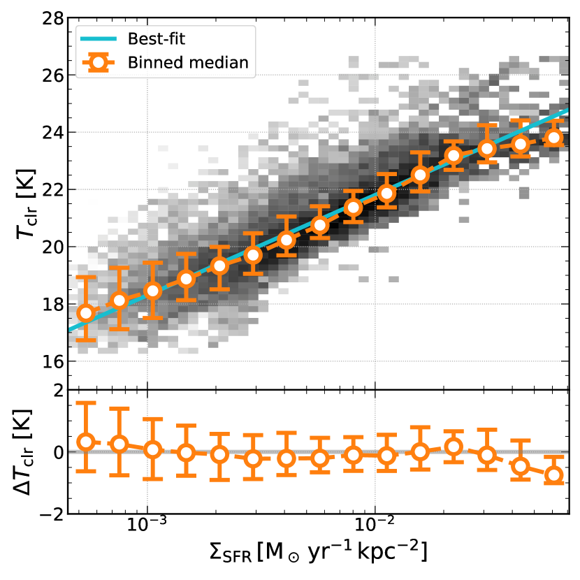
Figure 1: Measured scaling relation between ${T_{\mathrm{clr}}}$ and $\Sigma_{\mathrm{SFR}}$. Top panel: ${T_{\mathrm{clr}}}$ displayed as a function of $\Sigma_{\mathrm{SFR}}$. The gray scale shows the density of data points. The orange circles show the median ${T_{\mathrm{clr}}}$ in each $\Sigma_{\mathrm{SFR}}$ bin, and the errorbars show the 16th- and 84th-percentiles. The cyan line shows the best-fit power law between ${T_{\mathrm{clr}}}$ and $\Sigma_{\mathrm{SFR}}$ (equation 17). Bottom panel: $\Delta$${T_{\mathrm{clr}}}$ (defined in equation 18) displayed as a function of $\Sigma_{\mathrm{SFR}}$, with a gray line showing zero position.

In Table 2, we show Pearson’s correlation coefficient ($\rho$) between ${T_{\mathrm{clr}}}$ and each of the quantities available in our analysis. Since most quantities have certain radial dependence, we include $R_{\mathrm{g}}/R_{25}$ as a reference quantity. Quantities that have correlations with ${T_{\mathrm{clr}}}$ stronger than $R_{\mathrm{g}}/R_{25}$ are more likely to have first-order correlations with ${T_{\mathrm{clr}}}$. Among the quantities with correlation stronger than $R_{\mathrm{g}}/R_{25}$, $\Sigma_{\mathrm{SFR}}$ has the strongest correlation with ${T_{\mathrm{clr}}}$ ($\rho=0.89$, showing a strong correlation). This agrees with the baseline assumption in Paper I that the UV radiation from young stars is the dominant dust heating source in the majority of the sample. $\Sigma_{\mathrm{mol}}$, $\Sigma_{\mathrm{gas}}$, $\Sigma_{\mathrm{dust}}$, and $\Sigma_{\star}$ also have correlations with ${T_{\mathrm{clr}}}$ stronger than $R_{\mathrm{g}}/R_{25}$. For $\Sigma_{\mathrm{mol}}$ and $\Sigma_{\mathrm{gas}}$, both correlations likely result from their strong correlations with $\Sigma_{\mathrm{SFR}}$, i.e the KS law. The correlation between $\Sigma_{\star}$ and ${T_{\mathrm{clr}}}$ also likely result from the correlation between $\Sigma_{\star}$ and $\Sigma_{\mathrm{SFR}}$, possibly indicating the resolved star-forming main sequence (Cano-Díaz et al., 2016; Abdurro’uf & Akiyama, 2017, 2018; Hsieh et al., 2017; Liu et al., 2018; Maragkoudakis et al., 2017; Medling et al., 2018; Lin et al., 2019, 2022; Morselli et al., 2020; Ellison et al., 2021; Pessa et al., 2022). $\Sigma_{\mathrm{dust}}$ has a correlation slightly stronger than the radial dependence, which might result from its correlation with $\Sigma_{\mathrm{gas}}$ due to the relatively small D/G variations. Note that from the analysis in Paper I, we expect a negative correlation between $\Sigma_{\mathrm{dust}}$ and ${T_{\mathrm{clr}}}$ at fixed $\Sigma_{\mathrm{SFR}}$ because of the effect of dust shielding. We conversely observe a moderately positive correlation between $\Sigma_{\mathrm{dust}}$ and ${T_{\mathrm{clr}}}$ here, since with increasing $\Sigma_{\mathrm{dust}}$, $\Sigma_{\mathrm{SFR}}$ (or the UV radiation field) increases owing to the KS law.

We display ${T_{\mathrm{clr}}}$ as a function of $\Sigma_{\mathrm{SFR}}$ in the top panel of Fig. 1. As shown in the figure and implied from the correlation, the observed ${T_{\mathrm{clr}}}$ seems to have a power-law dependence on $\Sigma_{\mathrm{SFR}}$. The best-fit power-law relation is

$$\frac{{T_{\mathrm{clr}}}}{1~{}\mathrm{K}}=(3.50\pm 0.02)\log\Bigg{(}\frac{\Sigma_{\mathrm{SFR}}}{1~{}{\rm M_{\odot}\,yr}^{-1}\,{\rm kpc}^{-2}}\Bigg{)}+(28.81\pm 0.04)~{}.$$ (17)

The root-mean-square deviation (RMSD) between measured ${T_{\mathrm{clr}}}$ and the best-fit relation is 0.81 K. The residual between the measurements and best-fit relation $\Delta{T_{\mathrm{clr}}}$ is defined as

$$\Delta{T_{\mathrm{clr}}}\equiv T_{\mathrm{clr}}^{\mathrm{measured}}-T_{\mathrm{clr}}^{\mathrm{best\mbox{-}fit}}(\Sigma_{\mathrm{SFR}}),$$ (18)

where the first and second terms on the right-hand side are the measured and best-fit colour temperatures, respectively. We show $\Delta$${T_{\mathrm{clr}}}$ as a function of $\Sigma_{\mathrm{SFR}}$ in the bottom panel of Fig. 1. The residual $\Delta$${T_{\mathrm{clr}}}$ is centred around zero throughout almost the entire observed $\Sigma_{\mathrm{SFR}}$ range, again indicating the significance of the power-law relation between ${T_{\mathrm{clr}}}$ and $\Sigma_{\mathrm{SFR}}$. However, we do notice that there tends to be a larger scatter toward the low-$\Sigma_{\mathrm{SFR}}$ end, and larger deviation ($>0.5$ K) toward the high-$\Sigma_{\mathrm{SFR}}$ end.

Table 3: Correlation between $\Delta$${T_{\mathrm{clr}}}$ and local conditions. We calculate Pearson’s correlation coefficient ($\rho$) along with the $p$-value of the correlation.

Quantity	Pearson’s $\rho$ with $\Delta$${T_{\mathrm{clr}}}$	$p$-value
$\Sigma_{\mathrm{atom}}$	0.21	$\ll 0.001$
$\log(\Sigma_{\mathrm{mol}})$	-0.12	$\ll 0.001$
$\log(\Sigma_{\mathrm{gas}})$	-0.05	$\ll 0.001$
$\log(\Sigma_{\mathrm{dust}})$	-0.26	$\ll 0.001$
$\log(\mathrm{D/G})$	-0.27	$\ll 0.001$
$\log(\Sigma_{\star})$	0.06	$\ll 0.001$
12+$\log(\mathrm{O/H})$	-0.01	0.012
$R_{\mathrm{g}}/R_{25}$	-0.1	$\ll 0.001$

• Notes: (a) $\Delta$${T_{\mathrm{clr}}}$ is defined in equation (18). (b) $\Sigma_{\mathrm{SFR}}$ is excluded from this table because it has no correlation with $\Delta$${T_{\mathrm{clr}}}$, as expected. (c) We consider the correlation as significant when we have $p<0.05$.

To investigate the possible secondary dependence of ${T_{\mathrm{clr}}}$ on the local environment, we calculate the correlations between $\Delta$${T_{\mathrm{clr}}}$ and local conditions, and present them in Table 3. All the quantities show weak or no correlations with $\Delta$${T_{\mathrm{clr}}}$, indicating that there is no single secondary parameters that strongly affects ${T_{\mathrm{clr}}}$ throughout all observed samples.

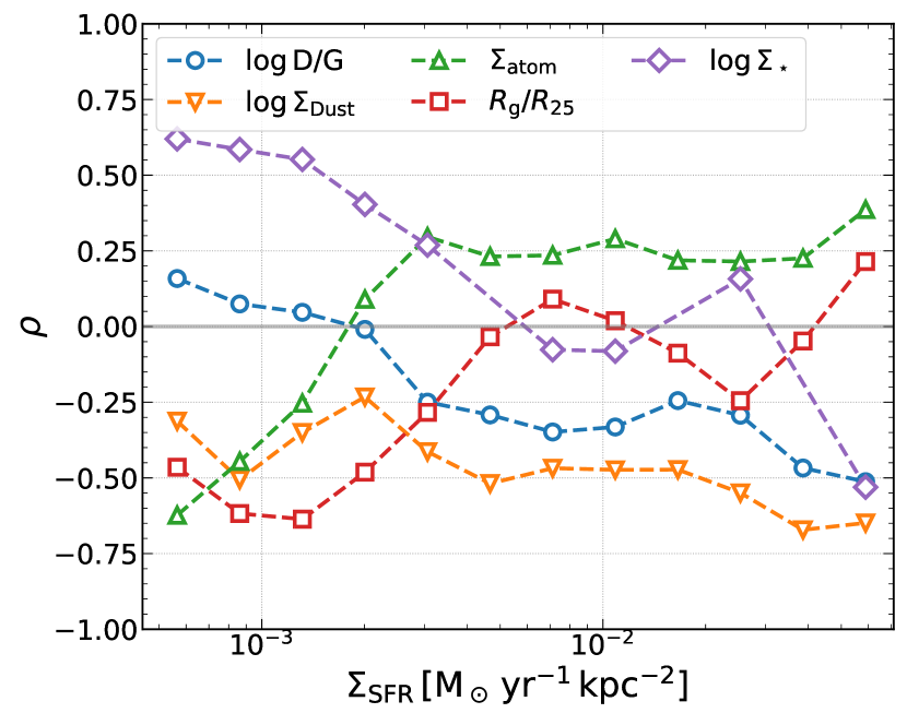
Figure 2: Pearson’s correlation coefficient ($\rho$) between $\Delta$${T_{\mathrm{clr}}}$ (equation 18) and selected local environment quantities in each $\Sigma_{\mathrm{SFR}}$ bin. Quantities made into this selection have their $|\rho|$ values exceeding 0.5 in at least one of the bins. We skip the bins with $p$-values greater than 0.05, which happens in a few high-$\Sigma_{\mathrm{SFR}}$ bins for $\log\Sigma_{\star}$.

To further approach the possible secondary dependence, we group the data points in bins of $\Sigma_{\mathrm{SFR}}$, and calculate the correlation between $\Delta$${T_{\mathrm{clr}}}$ and local conditions in each bin. The result is shown in Fig. 2, only keeping the quantities that have their $|\rho|>0.5$ in at least one of the $\Sigma_{\mathrm{SFR}}$ bins. D/G and $\Sigma_{\mathrm{dust}}$, which are expected to reduce ${T_{\mathrm{clr}}}$ due to increased opacity from the Paper I analysis, show stronger negative correlations with $\Delta$${T_{\mathrm{clr}}}$ toward higher $\Sigma_{\mathrm{SFR}}$. $\Sigma_{\mathrm{dust}}$ has a stronger correlation than D/G and the correlation coefficient is negative throughout the observed range, suggesting that $\Sigma_{\mathrm{dust}}$ traces the dust opacity effect on ${T_{\mathrm{clr}}}$ more directly in observations than D/G. On the other hand, D/G has a weak but positive correlation coefficient at low $\Sigma_{\mathrm{SFR}}$, which means that there are other mechanisms that cancel out the opacity effect traced by D/G.

The correlation between $\Delta$${T_{\mathrm{clr}}}$ and normalized radius is almost a mirror image of the one between $\Delta$${T_{\mathrm{clr}}}$ and $\log\Sigma_{\star}$, reflecting the fact that the radius normalized by $R_{25}$ correlates with $\log\Sigma_{\star}$, i.e. an exponential disc, in our sample. Similar to the case of D/G mentioned above, the correlation between $\Sigma_{\star}$ and $\Delta$${T_{\mathrm{clr}}}$ behaves differently at low and high $\Sigma_{\mathrm{SFR}}$. Below $\Sigma_{\mathrm{SFR}}\sim 2\times 10^{-3}~{}{\rm M_{\odot}\,yr}^{-1}\,{\rm kpc}^{-2}$, $\Sigma_{\star}$ positively correlates with $\Delta$${T_{\mathrm{clr}}}$. This positive correlation for $\Sigma_{\star}$ might indicate the dust heating contributed by old stellar population in the low-$\Sigma_{\mathrm{SFR}}$ region. At mid-$\Sigma_{\mathrm{SFR}}$ values, $\Sigma_{\star}$ weakly correlates with $\Delta$${T_{\mathrm{clr}}}$. The correlation between $\Sigma_{\star}$ and $\Delta$${T_{\mathrm{clr}}}$ jumps to moderately negative strength only at the highest-$\Sigma_{\mathrm{SFR}}$ bin, where the cause is unclear and is to be identified with future data focusing on high $\Sigma_{\mathrm{SFR}}$ regions. The reason for the correlation between $\Delta$${T_{\mathrm{clr}}}$ and $\Sigma_{\mathrm{atom}}$ is even more difficult to identify because it depends on various complicated factors such as the transition from atomic to molecular phases. $\Sigma_{\mathrm{atom}}$ has a moderately negative correlation with $\Delta$${T_{\mathrm{clr}}}$ at low $\Sigma_{\mathrm{SFR}}$, which quickly weakens as $\Sigma_{\mathrm{SFR}}$ increases. At mid- to high-$\Sigma_{\mathrm{SFR}}$ values, $\Sigma_{\mathrm{atom}}$ has a weak positive correlation with $\Delta$${T_{\mathrm{clr}}}$.

4.2 Scaling relation between the surface densities of SFR, gas mass, and dust mass

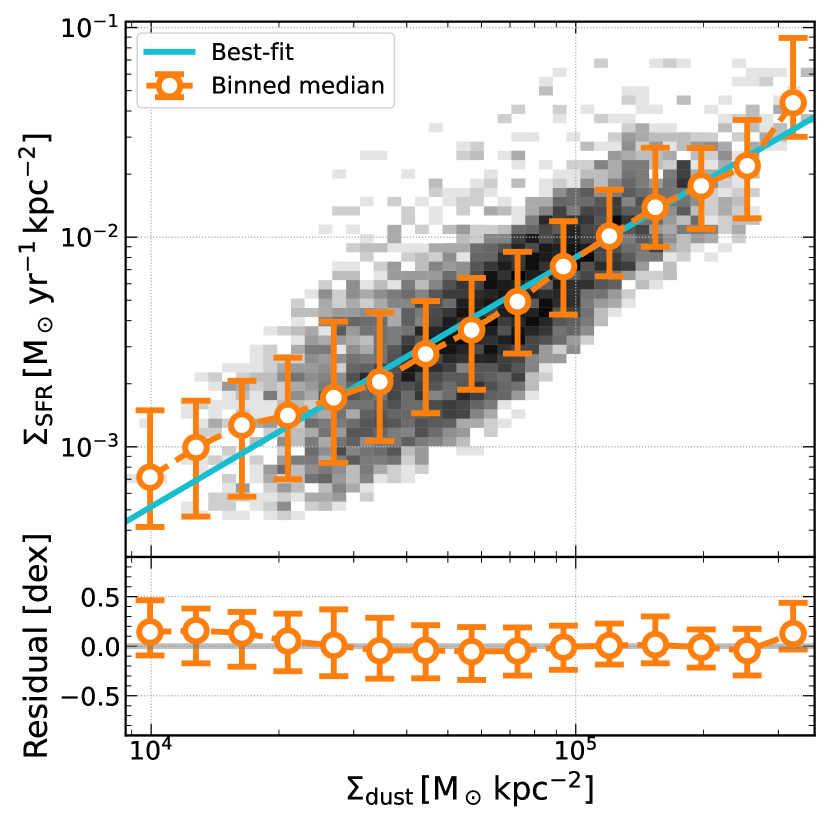
Figure 3: Measured scaling relation between $\Sigma_{\mathrm{SFR}}$ and $\Sigma_{\mathrm{dust}}$. Top panel: $\Sigma_{\mathrm{SFR}}$ displayed as a function of $\Sigma_{\mathrm{dust}}$. The gray scale shows the density of data points. The orange circles show the median $\Sigma_{\mathrm{SFR}}$ in each $\Sigma_{\mathrm{dust}}$ bin, and the error bars show the 16th- and 84th-percentiles. The cyan line shows the best-fit power law between $\Sigma_{\mathrm{SFR}}$ and $\Sigma_{\mathrm{dust}}$. Bottom panel: The residual, $\log(\Sigma_{\mathrm{SFR}}^{\mathrm{measured}})-\log(\Sigma_{\mathrm{SFR}}^{\mathrm{best\mbox{-}fit}})$ displayed as a function of $\Sigma_{\mathrm{dust}}$.

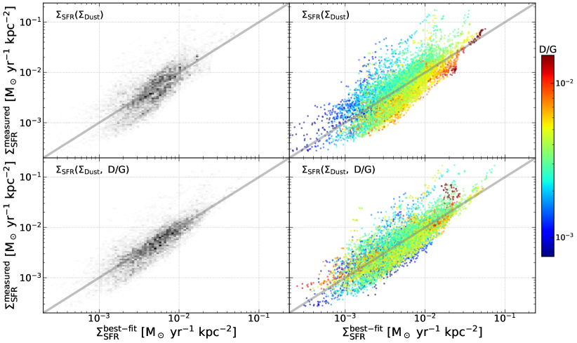
Figure 4: Comparison between measured $\Sigma_{\mathrm{SFR}}$ ($\Sigma_{\mathrm{SFR}}^{\mathrm{measured}}$) and $\Sigma_{\mathrm{SFR}}$ predicted from best-fit relations ($\Sigma_{\mathrm{SFR}}^{\mathrm{best\mbox{-}fit}}$) with $\Sigma_{\mathrm{dust}}$ alone (top panels) or with both $\Sigma_{\mathrm{dust}}$ and D/G (bottom panels). The left panels have their transparency indicating the distribution of data points, while the right panel shows the pixel-by-pixel data points colorized by D/G.

As mentioned in Section 3.4, an underlying assumption in the Paper I model is that at a given D/G, one can infer $\Sigma_{\mathrm{SFR}}$ from $\Sigma_{\mathrm{dust}}$ through the KS law (and $\Sigma_{\mathrm{gas}}$). Thus, in this subsection, we first present the measured relation between $\Sigma_{\mathrm{SFR}}$ and $\Sigma_{\mathrm{dust}}$ in Fig. 3. As shown in the figure, $\Sigma_{\mathrm{SFR}}$ is correlated with $\Sigma_{\mathrm{dust}}$. To build a reference for further comparison, we fit a power-law relation between the two. The best-fit relation is:

$$\log\Bigg{(}\frac{\Sigma_{\mathrm{SFR}}}{1~{}{\rm M_{\odot}\,yr}^{-1}\,{\rm kpc}^{-2}}\Bigg{)}=\\ (1.19\pm 0.01)\log\Bigg{(}\frac{\Sigma_{\mathrm{dust}}}{1~{}\rm M_{\odot}\,kpc\textsuperscript{-2}}\Bigg{)}-(8.05\pm 0.05).$$ (19)

The RMSD of this best-fit relation is 0.27 dex. The residual, $\log(\Sigma_{\mathrm{SFR}}^{\mathrm{measured}})-\log(\Sigma_{\mathrm{SFR}}^{\mathrm{best\mbox{-}fit}})$, has Pearson’s correlation coefficient of $-0.36$ with D/G, suggesting a medium trend that $\Sigma_{\mathrm{SFR}}$ increases toward regions with lower D/G at a given $\Sigma_{\mathrm{dust}}$. We compare the measured and best-fit $\Sigma_{\mathrm{SFR}}$ in the top-left panel of Fig. 4. Although we are able to get a solution minimizing the overall RMSD, the solution tends to underestimate $\Sigma_{\mathrm{SFR}}$ at high $\Sigma_{\mathrm{SFR}}$ and overestimate $\Sigma_{\mathrm{SFR}}$ at low $\Sigma_{\mathrm{SFR}}$. In other words, the $\log(\Sigma_{\mathrm{SFR}}^{\mathrm{best\mbox{-}fit}})$ has a smaller dynamical range than $\log(\Sigma_{\mathrm{SFR}}^{\mathrm{measured}})$.

Inspired by the design of the Paper I model, we investigate whether we can improve the prediction of $\Sigma_{\mathrm{SFR}}$ by including D/G as the second variable. This idea is supported by the top-right panel of Fig. 4, where we observe a systematic variation in D/G in the $\log(\Sigma_{\mathrm{SFR}}^{\mathrm{measured}})-\log(\Sigma_{\mathrm{SFR}}^{\mathrm{best\mbox{-}fit}})$ space. The best-fit $\Sigma_{\mathrm{SFR}}$ in a two-variable ($\Sigma_{\mathrm{dust}}$, D/G) fitting is

$$\log\Bigg{(}\frac{\Sigma_{\mathrm{SFR}}}{1~{}{\rm M_{\odot}\,yr}^{-1}\,{\rm kpc}^{-2}}\Bigg{)}=\\ (1.49\pm 0.01)\log\Bigg{(}\frac{\Sigma_{\mathrm{dust}}}{1~{}\rm M_{\odot}\,kpc\textsuperscript{-2}}\Bigg{)}-(0.73\pm 0.01)\log(\mathrm{D/G})\\ -(11.26\pm 0.07).$$ (20)

The RMSD of this best-fit decreases to 0.22 dex. In the bottom panels of Fig. 4, we use this fitting to the best-fit $\Sigma_{\mathrm{SFR}}$ ($\Sigma_{\mathrm{SFR}}^{\mathrm{best\mbox{-}fit}}$). We observe that $\Sigma_{\mathrm{SFR}}^{\mathrm{best\mbox{-}fit}}$ now traces the measurements better over the entire observed range, and the systematic trend of D/G in the $\log(\Sigma_{\mathrm{SFR}}^{\mathrm{measured}})-\log(\Sigma_{\mathrm{SFR}}^{\mathrm{best\mbox{-}fit}})$ space decreases.

With the best-fit result in equation (20), we claim that the assumption in Paper I, i.e. scaling of $\Sigma_{\mathrm{SFR}}$ with $\Sigma_{\mathrm{dust}}$ at given D/G, is consistent with our observation. To interpret the equation, we can convert $\Sigma_{\mathrm{dust}}$ in equation (20) to $\Sigma_{\mathrm{gas}}$ and D/G, i.e.

$$\log\Bigg{(}\frac{\Sigma_{\mathrm{SFR}}}{1~{}{\rm M_{\odot}\,yr}^{-1}\,{\rm kpc}^{-2}}\Bigg{)}\sim\\ 1.49\log\Bigg{(}\frac{\Sigma_{\mathrm{gas}}}{1~{}\rm M_{\odot}\,kpc\textsuperscript{-2}}\Bigg{)}+0.76\log(\mathrm{D/G})-11.26.$$ (21)

This functional form could be interpreted as a KS law with a correction term in D/G (hereafter D/G-modified KS law), with higher SFR toward larger D/G at given $\Sigma_{\mathrm{gas}}$. The 1.49 factor corresponds to the power-law index of KS law ($N$ in equation 16). This is consistent with the $N\sim 1.4$ value measured in Kennicutt (1998); de los Reyes & Kennicutt (2019) with total gas; meanwhile, our $N$ value is equal to or steeper than the values measured with molecular-gas-only KS law ($N_{\mathrm{H_{2}}}\sim 0.8$–1.5, Bigiel et al., 2008; Blanc et al., 2009; Rahman et al., 2011; Leroy et al., 2013; Kennicutt & De Los Reyes, 2021). The D/G correction term can cause an offset up to $\sim$0.8 dex in $\Sigma_{\mathrm{SFR}}$ with the observed D/G range ($\sim 10^{-3}$–$10^{-2}$), which is a significant change.

The D/G can influence the star formation activity through the formation of H₂ on dust surfaces (Krumholz et al., 2008, 2009; McKee & Krumholz, 2010). Such a condition may be favourable for star formation through the shielding of UV radiation by H₂ and dust at a given $\Sigma_{\mathrm{gas}}$. However, it is difficult to prove with our data that the D/G directly affects the star formation activity, because D/G is correlated with various other physical quantities that could affect star formation, such as metallicity, gas pressure, gravitational field, etc. We refer readers who are interested in how these physical quantities could affect SFR to the Kennicutt & Evans (2012) review.

5 Comparing to the Hirashita & Chiang (2022) model

5.1 Dependence of ${T_{\mathrm{clr}}}$ on the SFR surface density and D/G

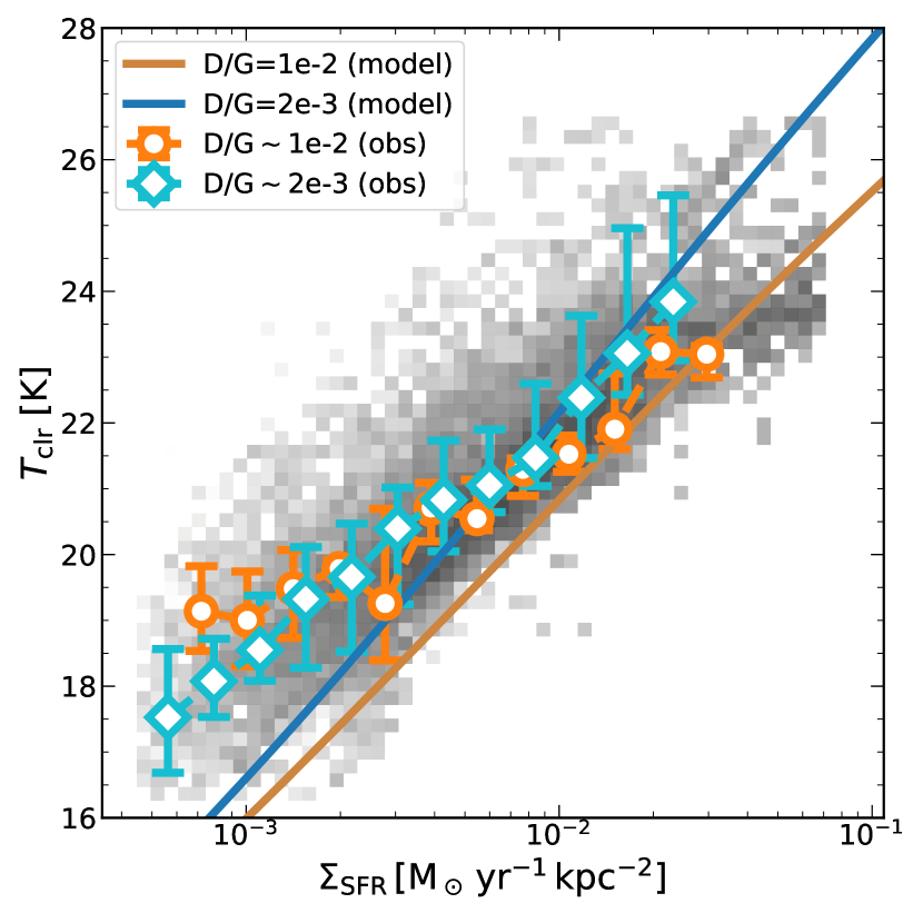
Figure 5: Comparison between the predicted and measured relations between ${T_{\mathrm{clr}}}$ and $\Sigma_{\mathrm{SFR}}$. The solid lines show the predicted ${T_{\mathrm{clr}}}$ at two D/G values ($\mathrm{D/G}=1.0\times 10^{-2}$ and $2.0\times 10^{-3}$ for brown and blue lines, respectively) from the Paper I model, calculated with coefficients in equation (21). The data points with error bars present the measured ${T_{\mathrm{clr}}}$ within $\pm 0.1$ dex of the desired D/G values ($1.0\times 10^{-2}$ and $2.0\times 10^{-3}$ for orange and cyan, respectively). The gray colour shows the distribution of all measurements (the same one shown in Fig. 1).

We display both measured and model-predicted ${T_{\mathrm{clr}}}$ as a function of $\Sigma_{\mathrm{SFR}}$ in Fig. 5. The predictions are calculated with the Paper I model, the set up descriptions in Section 3.4, and the coefficients in equation (21). From the Paper I model, we expect ${T_{\mathrm{clr}}}$ to increase with $\Sigma_{\mathrm{SFR}}$, and to increase with decreasing D/G at fixed $\Sigma_{\mathrm{SFR}}$, as shown in the blue and brown lines for $\mathrm{D/G}=1.0\times 10^{-2}$ and $2.0\times 10^{-3}$, respectively. To compare with this prediction, we select data points within $\pm 0.1$ dex of the two desired D/G values and plot them with connected data points with error bars in Fig. 5.

We observe that both the $\rm D/G\sim 1.0\times 10^{-2}$ and $\rm D/G\sim 2.0\times 10^{-3}$ groups follow the predicted trend at $\Sigma_{\mathrm{SFR}}\gtrsim 10^{-2}~{}{\rm M_{\odot}\,yr}^{-1}\,{\rm kpc}^{-2}$. Meanwhile, the separation of the two observed trends is not significant, with both groups falling within the $1\sigma$ scatter of data points of each other. At lower $\Sigma_{\mathrm{SFR}}$, the observed ${T_{\mathrm{clr}}}$ exceeds the model prediction. Moreover, the difference in ${T_{\mathrm{clr}}}$ between different D/G values become even less distinguishable. This implies that some assumptions made in Paper I might break down at low $\Sigma_{\mathrm{SFR}}$ as we will discuss in Section 5.3. Nevertheless, we emphasize that the Paper I model reproduces not only the overall trend but also the different relations for different values of D/G at $\Sigma_{\mathrm{SFR}}\gtrsim 10^{-2}~{}{\rm M_{\odot}\,yr}^{-1}\,{\rm kpc}^{-2}$.

5.2 Dependence of ${T_{\mathrm{clr}}}$ on the surface densities of SFR and dust

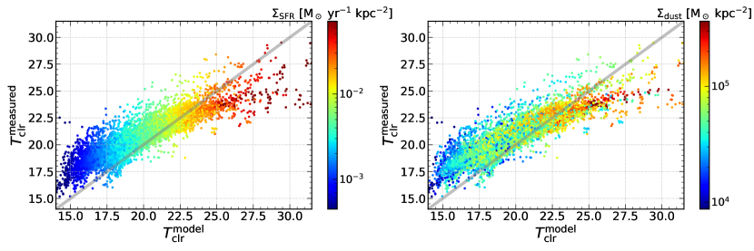
Figure 6: Measured and model-predicted ${T_{\mathrm{clr}}}$. The latter quantity, $T_{\mathrm{clr}}^{\mathrm{model}}$, is calculated with the measured pixel-by-pixel ($\Sigma_{\mathrm{SFR}}$, $\Sigma_{\mathrm{dust}}$) pair using the star formation law described in equation (21). The same data are plotted in the left and right panels, of which the data points are colour-coded by $\Sigma_{\mathrm{SFR}}$ and $\Sigma_{\mathrm{dust}}$, respectively.

One interesting conclusion in Paper I is that with $\Sigma_{\mathrm{SFR}}$ and $\Sigma_{\mathrm{dust}}$, one will be able to determine dust temperature (details in their Section 3.3). To test this with our data, we calculate ${T_{\mathrm{clr}}}$ from the measured $\Sigma_{\mathrm{SFR}}$ and $\Sigma_{\mathrm{dust}}$ in this work with the Paper I model, and compare the model-predicted ${T_{\mathrm{clr}}}$ to the measured one (the predicted data thus do not have matching $\Sigma_{\mathrm{gas}}$ and D/G with observations). As shown in Fig. 6, the measured ${T_{\mathrm{clr}}}$ ($T_{\mathrm{clr}}^{\mathrm{measured}}$) and model-predicted ${T_{\mathrm{clr}}}$ ($T_{\mathrm{clr}}^{\mathrm{model}}$) trace each other, with $\mathrm{RMSD}=1.6$ K. However, $T_{\mathrm{clr}}^{\mathrm{measured}}$ has a smaller dynamic range than $T_{\mathrm{clr}}^{\mathrm{model}}$. At ${T_{\mathrm{clr}}}\lesssim(\gtrsim)22.5$ K, the model tends to underestimate (overestimate) ${T_{\mathrm{clr}}}$. The difference at the highest-temperature end is possibly due to the scatter resulting from lack of measurements: although we have $\sim 16$ per cent of data points with $T_{\mathrm{clr}}^{\mathrm{measured}}>22.5$ K, only $\sim 2$ per cent of the data have $T_{\mathrm{clr}}^{\mathrm{measured}}>25$ K. As mentioned in Section 4.1, a larger sample focusing on high $\Sigma_{\mathrm{SFR}}$ (i.e. high ${T_{\mathrm{clr}}}$) is necessary to draw a firm conclusion for the dust properties at the high-${T_{\mathrm{clr}}}$ end. The difference in the low-temperature part connects back to the underestimation of ${T_{\mathrm{clr}}}$ in low-$\Sigma_{\mathrm{SFR}}$ regions described in Section 5.1. As shown in the left panel of Fig. 6, the threshold below which the model underestimates ${T_{\mathrm{clr}}}$ is near $\Sigma_{\mathrm{SFR}}\sim 10^{-2}~{}{\rm M_{\odot}\,yr}^{-1}\,{\rm kpc}^{-2}$, the same threshold we found in Section 5.1. The $T_{\mathrm{clr}}^{\mathrm{model}}$ has a correlation coefficient of $0.97$ with $\log\Sigma_{\mathrm{SFR}}$, $\sim 0.09$ higher than the one of $T_{\mathrm{clr}}^{\mathrm{measured}}$, indicating a slight overestimation of the role of $\Sigma_{\mathrm{SFR}}$ in dust heating in the model. On the other hand, $T_{\mathrm{clr}}^{\mathrm{model}}$ has a correlation coefficient of $0.67$ with $\log\Sigma_{\mathrm{dust}}$, $\sim 0.06$ higher than the one with $T_{\mathrm{clr}}^{\mathrm{measured}}$, indicating a possible underestimation of the strength of dust shielding.

5.3 Implications for the Hirashita & Chiang (2022) model

Through the various comparisons, we found that the analytical model proposed in Paper I successfully reproduced the first-order dependence of ${T_{\mathrm{clr}}}$ on $\Sigma_{\mathrm{SFR}}$. The predicted ${T_{\mathrm{clr}}}$ has correlation coefficients with $\Sigma_{\mathrm{SFR}}$ and $\Sigma_{\mathrm{dust}}$ quite similar to the observations. The predicted ${T_{\mathrm{clr}}}$ from $\Sigma_{\mathrm{SFR}}$ and $\Sigma_{\mathrm{dust}}$ traces the observed ${T_{\mathrm{clr}}}$, with a RMSD of 1.6 K.

The prediction of higher ${T_{\mathrm{clr}}}$ toward lower D/G at fixed $\Sigma_{\mathrm{SFR}}$ is less obvious in the observations. The phenomena are only seen above $\Sigma_{\mathrm{SFR}}\sim 10^{-2}~{}{\rm M_{\odot}\,yr}^{-1}\,{\rm kpc}^{-2}$ (or ${T_{\mathrm{clr}}}\sim 22.5$ K; Fig. 5). Below that, the model tends to underestimate ${T_{\mathrm{clr}}}$, and the observed ${T_{\mathrm{clr}}}$ is not sensitive to D/G at fixed $\Sigma_{\mathrm{SFR}}$. This suggests that there are physical mechanisms not modeled in the low-$\Sigma_{\mathrm{SFR}}$ region, which will be discussed below. However, this caveat will likely not affect the high-redshift applications, which the model was originally designed for, as high-redshift targets usually have $\Sigma_{\mathrm{SFR}}$ higher than the sample in this paper.

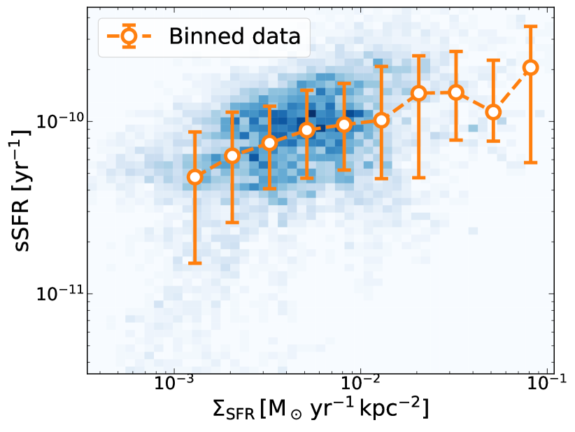
Figure 7: Relation between sSFR and $\Sigma_{\mathrm{SFR}}$ in our sample. The points connected by the dashed line show the median of sSFR in each $\Sigma_{\mathrm{SFR}}$ bin with the error bar showing the standard deviation, and the blue colour level shows the density of the pixel-by-pixel measurements on this diagram.

We raise three possible explanations for the higher observed temperature at low-$\Sigma_{\mathrm{SFR}}$. The first possibility is that the contribution to dust heating from old stars might be more important than assumed in the Paper I model (Groves et al., 2012; De Looze et al., 2014; Nersesian et al., 2019). For instance, Abdurro’uf et al. (2022b) showed, using a spatially resolved analysis of nearby galaxies, that the energy contribution from old stars to dust heating increases as sSFR decreases (see also Boquien et al., 2016; Leja et al., 2019). In Fig. 7, we show the measured sSFR as a function of $\Sigma_{\mathrm{SFR}}$. We observe that the sSFR becomes lower towards lower $\Sigma_{\mathrm{SFR}}$. This trend means that the fraction of young stars is up to three times lower comparing to old stars, not emitting UV radiation, at the lowest $\Sigma_{\mathrm{SFR}}$ bin. This observation suggests that the assumption of young-star-dominated heating is only applicable above certain threshold of $\Sigma_{\mathrm{SFR}}$, which is around $\Sigma_{\mathrm{SFR}}\sim 1\times 10^{-2}~{}{\rm M_{\odot}\,yr}^{-1}\,{\rm kpc}^{-2}$.

The second explanation is the difference in the stellar ages set by the model and traced by observations. In the model, we assume that the SFR is constant over the past $\tau_{\star}=10^{10}$ yr. However, our FUV and IR indicators only trace stars with age up to $\sim 10^{8}$ yr (see Kennicutt & Evans, 2012, and references therein). If the SFR at age > $10^{8}$ yr is higher than the current SFR (e.g. the decaying SFR in Nersesian et al., 2019), the constant-SFR model would underestimate the dust heating contributed from old ($>10^{8}$ yr) stellar populations and thus the dust temperature.

The above two possibilites can be tested by adding a stellar SED of an old stellar population to the Paper I model. For the purpose of this test, we add a stellar SED generated by starburst99 with an instantaneous burst occurring 1 Gyr ago, which is old enough not to contribute to the observed SFR, but young enough to contribute significantly to the dust temperature. Moreover, we choose the total stellar mass formed by this instantaneous burst two times larger than the original component (formed by a constant SFR over time), so that the sSFR is roughly three times lower. As a consequence, the dust temperature at $\Sigma_{\mathrm{SFR}}=10^{-3}$ ${\rm M_{\odot}\,yr}^{-1}\,{\rm kpc}^{-2}$ is raised to 18 and 19 K for $\mathrm{D/G}=10^{-2}$ and $2\times 10^{-3}$, respectively (originally $\sim 16$ K). These temperatures are consistent with the observed values, thus supporting the contribution from old stellar population as a reason for the higher dust temperatures in the observations than in the Paper I model. Since the old stellar population contributes to emission at longer wavelengths, its emission is less affected by dust extinction. This may also explain the small difference between the two cases of D/G values at low $\Sigma_{\mathrm{SFR}}$.

The third explanation we bring up is the spatial distribution of dust. In the Paper I model, we assume a uniform distribution of dust and stars in the plane of the galaxy disc, and adopt a thin-disc approximation. However, it is possible that in the outer disc, dust is less localized with young stars. This is supported by the residual shown in Fig. 3: in the low-$\Sigma_{\mathrm{SFR}}$ region, the observation deviates toward higher $\Sigma_{\mathrm{SFR}}$ per $\Sigma_{\mathrm{dust}}$, in other words, lower $\Sigma_{\mathrm{dust}}$ at fixed $\Sigma_{\mathrm{SFR}}$. This trend effectively lowers down the dust opacity and could raise the dust temperature. Alton et al. (1998), Bianchi (2007), Muñoz-Mateos et al. (2009a) and Hunt et al. (2015a) also showed that the exponential scale length of dust is longer (more extensive) than the one of stars. However, we remind the readers that there are also literature showing consistent spatial distribution between dust and FUV, e.g. Casasola et al. (2017) showed that $\Sigma_{\mathrm{dust}}$ and $I_{\mathrm{FUV}}$ have almost identical mean scale lengths ($h\sim 0.4R_{25}$) in the DustPedia sample.

6 Summary

In this work, we investigate the spatially resolved properties of dust temperature in nearby galaxies. We examine how the dust temperature is regulated by the surface densities of various quantities such as $\Sigma_{\mathrm{SFR}}$, $\Sigma_{\mathrm{dust}}$, and $\Sigma_{\mathrm{gas}}$, with both observations and model predictions. To achieve this goal, we compile multi-wavelength observations of dust, stars and SFR in 46 nearby galaxies, and make a 2 kpc scale map of each component. We measure how dust temperature (the 250 µm-to-100 µm colour temperature) scales with local physical conditions, and then compare our measurements to the dust temperature model developed by Paper I. We find the following features for the measured dust properties:

• The measured ${T_{\mathrm{clr}}}$ correlates well with spatially resolved $\Sigma_{\mathrm{SFR}}$. The best-fit power law yields a RMSD of 0.81 K.

• None of the measured quantities has an overall strong correlation with the residual of the above power-law fitting, $\Delta$${T_{\mathrm{clr}}}$. When analyzed in each $\Sigma_{\mathrm{SFR}}$ bin, we find some trends: Both D/G and $\Sigma_{\mathrm{dust}}$ have stronger negative correlations with $\Delta$${T_{\mathrm{clr}}}$ at mid to high $\Sigma_{\mathrm{SFR}}$, meaning that the effect of lower ${T_{\mathrm{clr}}}$ due to increased dust opacity is stronger at high-$\Sigma_{\mathrm{SFR}}$ regions.

• We provide an empirical formula to predict $\Sigma_{\mathrm{SFR}}$ with $\Sigma_{\mathrm{dust}}$ and D/G (equation 20). This is equivalent to a KS law modified by a secondary dependence on D/G.

Here is the summary of our key findings by comparing the measured dust temperature to the one predicted with the Paper I analytical dust temperature model:

• Our observations show that ${T_{\mathrm{clr}}}$ strongly correlates with $\Sigma_{\mathrm{SFR}}$ and that at fixed $\Sigma_{\mathrm{SFR}}$, ${T_{\mathrm{clr}}}$ increases as D/G decreases at $\Sigma_{\mathrm{SFR}}\gtrsim 1.0\times 10^{-2}~{}{\rm M_{\odot}\,yr}^{-1}\,{\rm kpc}^{-2}$. These results are consistent with the Paper I model. The latter is interpreted as less dust shielding in a dust-poor environment.

• The ${T_{\mathrm{clr}}}$ predicted from $\Sigma_{\mathrm{SFR}}$ and $\Sigma_{\mathrm{dust}}$ by the Paper I model using the newly derived star formation relation is reasonably consistent with observations, with a RMSD of 1.6 K. However, we observe a weaker dependence of ${T_{\mathrm{clr}}}$ on $\Sigma_{\mathrm{SFR}}$ with our measurements.

• At low $\Sigma_{\mathrm{SFR}}$ ($\lesssim 10^{-2}$ ${\rm M_{\odot}\,yr}^{-1}\,{\rm kpc}^{-2}$), our observed ${T_{\mathrm{clr}}}$ is higher than the prediction from the Paper I model, and it has no significant dependence on D/G. This is likely due to the contribution of dust heating from old stellar population and/or the variation of SFR within the past $10^{10}$ yr.

We conclude that the dust temperature reasonably scales with $\Sigma_{\mathrm{SFR}}$. At high-$\Sigma_{\mathrm{SFR}}$, the ${T_{\mathrm{clr}}}$ at fixed $\Sigma_{\mathrm{SFR}}$ decreases as D/G increases, which means that the Paper I model is consistent with observations at $\Sigma_{\mathrm{SFR}}\gtrsim 10^{-2}~{}{\rm M_{\odot}\,yr}^{-1}\,{\rm kpc}^{-2}$. Thus, we confirm that dust heating from young stars and shielding of radiation by dust regulate the dust temperature. We also propose a prescription to predict $\Sigma_{\mathrm{SFR}}$ from $\Sigma_{\mathrm{gas}}$ and D/G, i.e. a D/G-modified KS law. In the end, we succeed in obtaining a comprehensive understanding for the relations among dust temperature, dust content and star formation activity.

Data Availability

Data related to this publication and its figures are available on reasonable request from the corresponding author.

Appendix A Consistency between dust temperature tracers

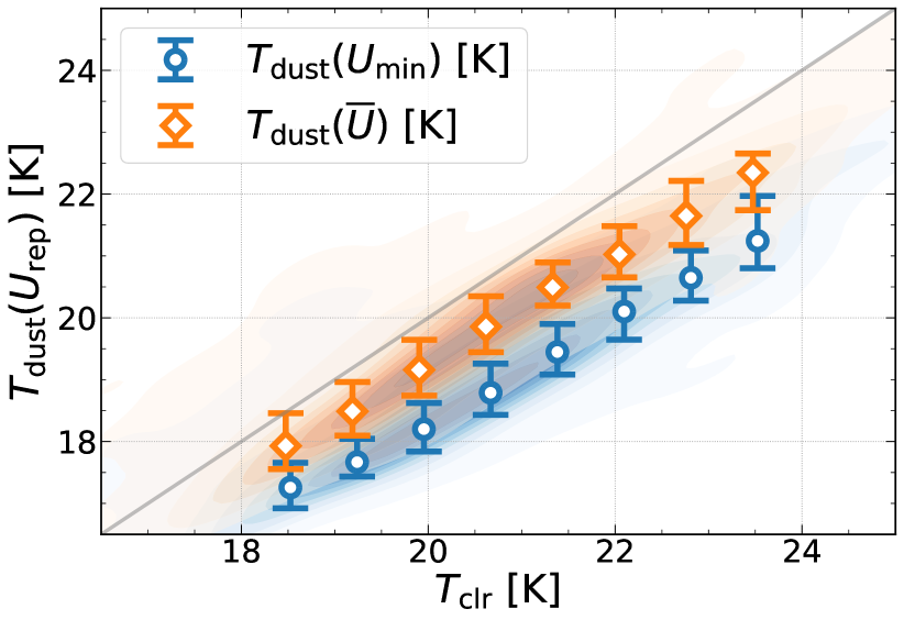
Figure 8: Comparison between the dust temperature tracers. The horizontal axis shows ${T_{\mathrm{clr}}}$, the FIR-based single dust temperature. The vertical axis presents ${T_{\mathrm{dust}}}(U_{\mathrm{rep}})$, the effective temperature converted from the ISRF distribution function. The blue shades show the density plot of pixel-by-pixel measurements of ${T_{\mathrm{dust}}(U_{\mathrm{min}})}$, and the blue line shows the median in each ${T_{\mathrm{clr}}}$ bin. The orange shades and line show the counterparts for ${T_{\mathrm{dust}}(\overline{U})}$.

In our analysis, we use ${T_{\mathrm{clr}}}$ as the fiducial tracer for dust temperature. There are other commonly used tracers for dust temperature that can be derived from dust SED fitting. Broadly, there are two different approaches: (1) the single temperature derived from the modified blackbody model (Schwartz, 1982; Hildebrand, 1983), which focuses on the emission in the FIR from large grains in radiative equilibrium and (2) the effective temperature derived from the distribution function of ISRF, which is a product of SED fitting with a physical dust model (e.g. Dale et al., 2001; Draine & Li, 2007). The latter usually includes the non-equilibrium thermal emission from small grains. In this section, we briefly examine the consistency between these two approaches, i.e. the colour temperature (${T_{\mathrm{clr}}}$) introduced in the main text, which focuses on the equilibrium emission in the FIR thus belongs to the first approach, and the ISRF strength from SED fitting results in $z$0MGS (J. Chastenet et al. in preparation, fitting done with the Draine & Li, 2007, model), which belongs to the second method.

In the Draine & Li (2007) model, the scaled ISRF intensity is denoted as $U$, expressed in units of the MW diffuse ISRF at 10 kpc from Mathis et al. (1983). The ISRF contributing to dust heating is described by a combination of two components: a fraction of dust mass ($\gamma$) heated by a power-law distribution ($\propto U^{-\alpha}$) of starlight with $U_{\mathrm{min}}\leq U\leq U_{\mathrm{max}}$ (Dale et al., 2001), and the rest ($1-\gamma$) of dust mass heated by $U=U_{\mathrm{min}}$, i.e. diffuse ISM radiation.

J. Chastenet et al. (in preparation) fix $\alpha=2$ and $U_{\mathrm{max}}=10^{7}$, and leaves $\gamma$ and $U_{\mathrm{min}}$ as free parameters (following Aniano et al., 2012, 2020). According to Draine et al. (2014), we can convert a representative ISRF ($U_{\mathrm{rep}}$) to a representative dust temperature with:

$$\frac{{T_{\mathrm{dust}}}(U_{\mathrm{rep}})}{1~{}\rm K}=18\times U_{\mathrm{rep}}^{1/6}~{}.$$ (22)

There are two commonly used conventions for $U_{\mathrm{rep}}$. One is $U_{\mathrm{rep}}=U_{\mathrm{min}}$ by assuming that the majority of dust mass is heated by $U_{\mathrm{min}}$, i.e. $\gamma\ll 1$. This assumption is true almost throughout the entire M101 (Chastenet et al., 2021) and regions with high dust luminosity surface density (Aniano et al., 2012; Chastenet et al., 2021). The other convention adopts the dust-mass-averaged ISRF, $\overline{U}$, as $U_{\mathrm{rep}}$. The functional form of $\overline{U}$ is:

$$\overline{U}=(1-\gamma)U_{\mathrm{min}}+\gamma U_{\mathrm{min}}\frac{\ln(U_{\mathrm{max}}/U_{\mathrm{min}})}{1-(U_{\mathrm{min}}/U_{\mathrm{max}})}~{}~{}~{}\text{for $\alpha=2$}.$$ (23)

With that said, the three ${T_{\mathrm{dust}}}$ tracers we will compare here are: ${T_{\mathrm{clr}}}$, ${T_{\mathrm{dust}}}(U_{\mathrm{min}})$ and ${T_{\mathrm{dust}}}(\overline{U})$ (equations 3, 22 and 23). As shown in Fig. 8, the three tracers are roughly parallel to each other in the temperature range of interest, suggesting that these temperature tracers reasonably trace each other with a possible systematic offset in the calibration between ${T_{\mathrm{clr}}}$ and the representative ${T_{\mathrm{dust}}}$ converted from the ISRF strength. ${T_{\mathrm{clr}}}$ is systematically $\sim 0.8~{}\rm K$ and $\sim 1.8~{}\rm K$ higher than ${T_{\mathrm{dust}}(\overline{U})}$ and ${T_{\mathrm{dust}}(U_{\mathrm{min}})}$, respectively. The fact that ${T_{\mathrm{dust}}(\overline{U})}$ is consistently higher than ${T_{\mathrm{dust}}(U_{\mathrm{min}})}$ suggests that the hotter dust component, which is represented by the power-law component in the Draine & Li (2007) formulation, is important in the model. The $\sim 0.4~{}\rm K$ ($\sim 2\%$ in ${T_{\mathrm{dust}}}$, or $\sim 0.05$ dex in $U$) offset between ${T_{\mathrm{clr}}}$ and ${T_{\mathrm{dust}}(\overline{U})}$ is roughly 2.5 times the typical uncertainty in $\overline{U}$ from J. Chastenet et al. (in preparation, $\sigma\sim 0.02~{}\mathrm{dex}$), which indicates that this offset is significant.

Appendix B Robustness under the adopted CO-to-H₂ conversion factors

As we mentioned in Section 3.2, how the CO-to-H₂ conversion factor, $\alpha_{\rm CO}$, depends on local conditions is still an active field of study. In our main analysis, we calculate $\alpha_{\rm CO}$ with the prescription suggested by Bolatto et al. (2013), because it is one of the few prescriptions that formulate both the CO-dark molecular gas and the decrease of $\alpha_{\rm CO}$ in galaxy centres, where the latter has been proved to be necessary to obtain reasonable values for D/G and D/M (Chiang et al., 2021). Meanwhile, Sun et al. (2020) suggested that the exponential dependence on metallicity in the Bolatto et al. (2013) prescription might overestimate $\alpha_{\rm CO}$ in low-metallicity regions. Besides an exponential dependence, it is a commonly used strategy to formulate $\alpha_{\rm CO}$ as a power-law of metallicity (e.g. Glover & Mac Low, 2011; Schruba et al., 2012; Hunt et al., 2015b). In this section, we examine how our findings might change with different $\alpha_{\rm CO}$ prescriptions. Specifically, we will examine (1) how the correlation between $\Delta$${T_{\mathrm{clr}}}$ and D/G changes with $\alpha_{\rm CO}$ (Sections 4.1 and 5.1), and (2) whether the D/G modification to the KS law still makes sense (Section 4.2).

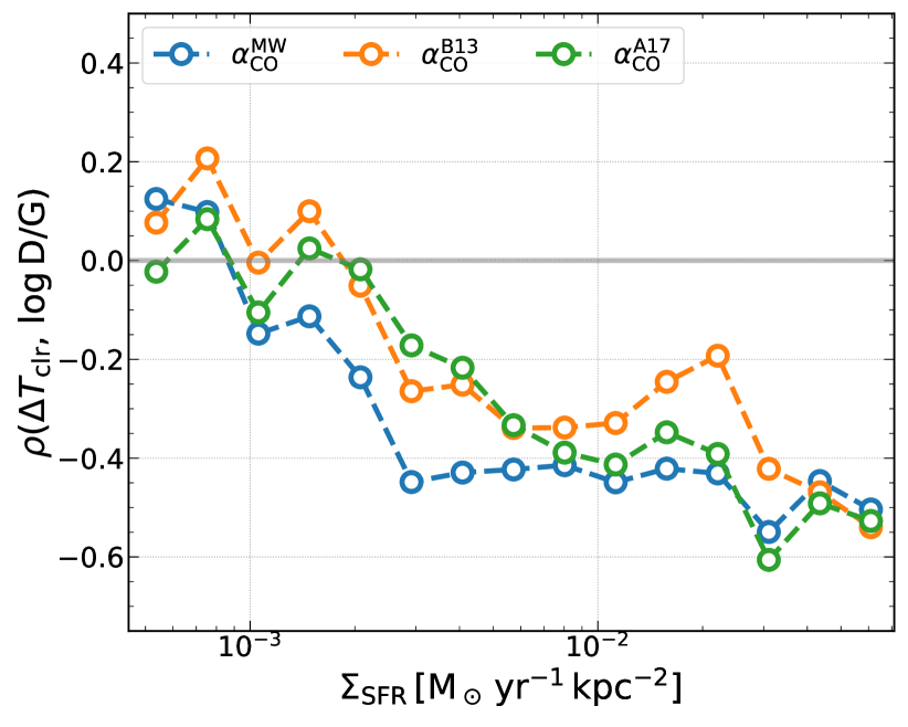
Figure 9: Pearson’s correlation coefficient ($\rho$) between $\Delta$${T_{\mathrm{clr}}}$ and $\log\mathrm{(D/G)}$ calculated with different $\alpha_{\rm CO}$ prescriptions.

We adopt three $\alpha_{\rm CO}$ prescriptions here: a constant $\alpha_{\rm CO}$, an $\alpha_{\rm CO}$ that depends on metallicity exponentially, and an $\alpha_{\rm CO}$ that depends on metallicity with a power law. For the constant one, we adopt the $\alpha_{\rm CO}$ in typical giant molecular clouds (GMCs) in the MW disc, $\alpha_{\rm CO}^{\rm MW}=4.35~{}{\rm M_{\odot}\,pc^{-2}\,(K\,km\,s^{-1})^{-1}}$ (Solomon et al., 1987; Strong & Mattox, 1996; Abdo et al., 2010). We use the Bolatto et al. (2013) prescription (equation 14) for the exponential one. Lastly, we adopt the power-law prescription suggested by Accurso et al. (2017), who used the [C ii] to CO $J=1\to 0$ ratio to constrain $\alpha_{\rm CO}$ and obtained the following metallicity-dependent conversion factor:

$$\frac{\alpha_{\rm CO}^{\rm A17}}{1~{}{\rm M_{\odot}\,pc^{-2}\,(K\,km\,s^{-1})^{-1}}}=4.35\,Z^{\prime-1.6}.$$ (24)

Note that we neglect the dependence on the offset from the main sequence in the Accurso et al. (2017) formulation, following the approach in Sun et al. (2020).

In addition to $\alpha_{\rm CO}$, we also examine how the variation in the CO line ratio, $R_{21}$ (equation 1), might affect our results. We adopt the SFR-dependent formula proposed in Leroy et al. (2022, see their Table 5), that is:

$$\log\bigg{(}\frac{R_{21}}{\langle R_{21}\rangle_{\mathrm{gal}}}\bigg{)}=0.129\log\bigg{(}\frac{\Sigma_{\mathrm{SFR}}}{\langle\Sigma_{\mathrm{SFR}}\rangle_{\mathrm{gal}}}\bigg{)}+0.019,$$ (25)

where the $\langle\rangle_{\mathrm{gal}}$ symbol represents the average value in the disc of each galaxy. For simplicity, we use $\langle R_{21}\rangle_{\mathrm{gal}}=0.65$ for all galaxies, and we adopt the geometric mean of the SFR surface densities for all pixels within a galaxy for $\langle\Sigma_{\mathrm{SFR}}\rangle_{\mathrm{gal}}$. Following the suggestion in Leroy et al. (2022), if the derived $R_{21}$ is greater than 1.0, we directly set it to 1.0.

We first re-calculate the correlation between $\Delta$${T_{\mathrm{clr}}}$ (Section 4.1) and $\log(\mathrm{D/G})$ with the three $\alpha_{\rm CO}$ prescriptions. The correlation coefficients are calculated for each $\Sigma_{\mathrm{SFR}}$ bin. Compared to Fig. 2, we only keep D/G because it is the only quantity affected by the choice of $\alpha_{\rm CO}$. As shown in Fig. 9, the correlation coefficients as a function of $\Sigma_{\mathrm{SFR}}$ have similar behaviours for the three $\alpha_{\rm CO}$ prescriptions. They all show poor correlation at low $\Sigma_{\mathrm{SFR}}$, and the correlations become stronger toward high $\Sigma_{\mathrm{SFR}}$. The two metallicity-dependent $\alpha_{\rm CO}$ prescriptions have similar transition $\Sigma_{\mathrm{SFR}}$ from poor to stronger correlation. Thus, as long as we use a metallicity-dependent $\alpha_{\rm CO}$, we expect ${T_{\mathrm{clr}}}$ to have poor correlation with D/G at low $\Sigma_{\mathrm{SFR}}$. The correlations between $\Delta$${T_{\mathrm{clr}}}$ and $\log(\mathrm{D/G})$ calculated with varying $R_{21}$ (equation 25) does not deviate significantly from the constant $R_{21}$ results.

Table 4: The RMSD (in dex) of the power-law fittings to $\Sigma_{\mathrm{SFR}}$ using different sets of variables for the three $\alpha_{\rm CO}$ prescriptions. For the fitting with two variables ($\Sigma_{\mathrm{dust}}$ and D/G), we examine two cases for $R_{21}$. See Section 4.2 for fitting formulation.

Formulation	$\alpha_{\rm CO}^{\rm MW}$	$\alpha_{\rm CO}^{\rm B13}$	$\alpha_{\rm CO}^{\rm A17}$
$\Sigma_{\mathrm{SFR}}$ ($\Sigma_{\mathrm{dust}}$)	0.27	–	–
$\Sigma_{\mathrm{SFR}}$ ($\Sigma_{\mathrm{dust}}$, D/G), constant $R_{21}$	0.20	0.22	0.22
$\Sigma_{\mathrm{SFR}}$ ($\Sigma_{\mathrm{dust}}$, D/G), varying $R_{21}$	0.22	0.24	0.24

• Note: There is no $\alpha_{\rm CO}$ involved in the $\Sigma_{\mathrm{SFR}}$ ($\Sigma_{\mathrm{dust}}$) fitting.

Next, we examine the power-law fittings to $\Sigma_{\mathrm{SFR}}$ similar to what we have done in Section 4.2 with $\alpha_{\rm CO}^{\rm B13}$. In Table 4, we present the RMSD of all the power-law fittings in this test. We test three formulations: the $\Sigma_{\mathrm{SFR}}$ ($\Sigma_{\mathrm{dust}}$) and $\Sigma_{\mathrm{SFR}}$ ($\Sigma_{\mathrm{dust}}$, D/G) with constant $R_{21}$, which we have performed in Section 4.2, and $\Sigma_{\mathrm{SFR}}$ ($\Sigma_{\mathrm{dust}}$, D/G) with varying $R_{21}$ in addition. As shown in Table 4, all the three $\alpha_{\rm CO}$ prescriptions show improved RMSD when moving from single-variable power law to the two-variable power law (constant $R_{21}$), indicating that the D/G-modification to the standard KS law (equation 21) is supported robustly against the change of the $\alpha_{\rm CO}$ prescriptions. Meanwhile, the two-variable power law with varying $R_{21}$ has systematically larger RMSD than the constant $R_{21}$ ones, showing the variation of $R_{21}$ does not improve the fitting.

When we interpret the two-variable power law as a D/G-modification to the standard KS law (equation 21) with different $\alpha_{\rm CO}$ prescriptions, we find the coefficient for the $\log\Sigma_{\mathrm{gas}}$ term (corresponding to the $N$ value in the standard KS law) as 1.35 for $\alpha_{\rm CO}^{\rm A17}$ and 1.39 for $\alpha_{\rm CO}^{\rm MW}$, both lower than the 1.49 for $\alpha_{\rm CO}^{\rm B13}$. Meanwhile, we have similar coefficients for the $\log(\mathrm{D/G})$ term for the metallicity-dependent prescriptions: 0.72 for $\alpha_{\rm CO}^{\rm A17}$ and 0.76 for $\alpha_{\rm CO}^{\rm B13}$. On the other hand, the coefficient for the constant $\alpha_{\rm CO}^{\rm MW}$ is 0.48, which yields a weaker correction than the metallicity-dependent $\alpha_{\rm CO}$ prescriptions.

References

- Abdo et al. (2010) Abdo A. A., et al., 2010, ApJ, 710, 133
- Abdurro’uf & Akiyama (2017) Abdurro’uf Akiyama M., 2017, MNRAS, 469, 2806
- Abdurro’uf & Akiyama (2018) Abdurro’uf Akiyama M., 2018, MNRAS, 479, 5083
- Abdurro’uf et al. (2022a) Abdurro’uf et al., 2022a, ApJS, 259, 35
- Abdurro’uf et al. (2022b) Abdurro’uf Lin Y.-T., Hirashita H., Morishita T., Tacchella S., Akiyama M., Takeuchi T. T., Wu P.-F., 2022b, ApJ, 926, 81
- Accurso et al. (2017) Accurso G., et al., 2017, MNRAS, 470, 4750
- Alton et al. (1998) Alton P. B., et al., 1998, A&A, 335, 807
- Aniano et al. (2011) Aniano G., Draine B. T., Gordon K. D., Sandstrom K., 2011, PASP, 123, 1218
- Aniano et al. (2012) Aniano G., et al., 2012, ApJ, 756, 138
- Aniano et al. (2020) Aniano G., et al., 2020, ApJ, 889, 150
- Asplund et al. (2009) Asplund M., Grevesse N., Sauval A. J., Scott P., 2009, ARA&A, 47, 481
- Astropy Collaboration et al. (2013) Astropy Collaboration et al., 2013, A&A, 558, A33
- Astropy Collaboration et al. (2018) Astropy Collaboration et al., 2018, AJ, 156, 123
- Astropy Collaboration et al. (2022) Astropy Collaboration et al., 2022, ApJ, 935, 167
- Bakx et al. (2021) Bakx T. J. L. C., et al., 2021, MNRAS, 508, L58
- Barrera-Ballesteros et al. (2016) Barrera-Ballesteros J. K., et al., 2016, MNRAS, 463, 2513
- Barrera-Ballesteros et al. (2021) Barrera-Ballesteros J. K., et al., 2021, MNRAS, 503, 3643
- Bendo et al. (2012) Bendo G. J., et al., 2012, MNRAS, 419, 1833
- Bendo et al. (2015) Bendo G. J., et al., 2015, MNRAS, 448, 135
- Bernstein et al. (2002) Bernstein R. A., Freedman W. L., Madore B. F., 2002, ApJ, 571, 56
- Bianchi (2007) Bianchi S., 2007, A&A, 471, 765
- Bianchi et al. (2018) Bianchi S., et al., 2018, A&A, 620, A112
- Bigiel et al. (2008) Bigiel F., Leroy A., Walter F., Brinks E., de Blok W. J. G., Madore B., Thornley M. D., 2008, AJ, 136, 2846
- Blanc et al. (2009) Blanc G. A., Heiderman A., Gebhardt K., Evans Neal J. I., Adams J., 2009, ApJ, 704, 842
- Bolatto et al. (2013) Bolatto A. D., Wolfire M., Leroy A. K., 2013, ARA&A, 51, 207
- Boquien et al. (2016) Boquien M., et al., 2016, A&A, 591, A6
- Bouwens et al. (2016) Bouwens R. J., et al., 2016, ApJ, 833, 72
- Braun et al. (2009) Braun R., Thilker D. A., Walterbos R. A. M., Corbelli E., 2009, ApJ, 695, 937
- Buat et al. (2005) Buat V., et al., 2005, ApJ, 619, L51
- Buat et al. (2012) Buat V., et al., 2012, A&A, 545, A141
- Burgarella et al. (2020) Burgarella D., Nanni A., Hirashita H., Theulé P., Inoue A. K., Takeuchi T. T., 2020, A&A, 637, A32
- Calzetti (2001) Calzetti D., 2001, PASP, 113, 1449
- Cano-Díaz et al. (2016) Cano-Díaz M., et al., 2016, ApJ, 821, L26
- Capak et al. (2015) Capak P. L., et al., 2015, Nature, 522, 455
- Casasola et al. (2017) Casasola V., et al., 2017, A&A, 605, A18
- Casasola et al. (2022) Casasola V., et al., 2022, A&A, 668, A130
- Cazaux & Tielens (2004) Cazaux S., Tielens A. G. G. M., 2004, ApJ, 604, 222
- Chastenet et al. (2021) Chastenet J., et al., 2021, ApJ, 912, 103
- Chiang (2021) Chiang I.-D., 2021, PhD thesis, University of California San Diego
- Chiang et al. (2018) Chiang I.-D., Sandstrom K. M., Chastenet J., Johnson L. C., Leroy A. K., Utomo D., 2018, ApJ, 865, 117
- Chiang et al. (2021) Chiang I.-D., et al., 2021, ApJ, 907, 29
- Compiègne et al. (2011) Compiègne M., et al., 2011, A&A, 525, A103
- Corbelli et al. (2010) Corbelli E., Lorenzoni S., Walterbos R., Braun R., Thilker D., 2010, A&A, 511, A89
- Dale et al. (2001) Dale D. A., Helou G., Contursi A., Silbermann N. A., Kolhatkar S., 2001, ApJ, 549, 215
- Dale et al. (2012) Dale D. A., et al., 2012, ApJ, 745, 95
- Davies et al. (2017) Davies J. I., et al., 2017, PASP, 129, 044102
- De Looze et al. (2014) De Looze I., et al., 2014, A&A, 571, A69
- de Blok et al. (2008) de Blok W. J. G., Walter F., Brinks E., Trachternach C., Oh S.-H., Kennicutt R. C., 2008, AJ, 136, 2648
- Desert et al. (1990) Desert F.-X., Boulanger F., Puget J. L., 1990, A&A, 237, 215
- Draine (2003) Draine B. T., 2003, ApJ, 598, 1017
- Draine & Li (2007) Draine B. T., Li A., 2007, ApJ, 657, 810
- Draine et al. (2014) Draine B. T., et al., 2014, ApJ, 780, 172
- Druard et al. (2014) Druard C., et al., 2014, A&A, 567, A118
- Ellison et al. (2021) Ellison S. L., Lin L., Thorp M. D., Pan H.-A., Scudder J. M., Sánchez S. F., Bluck A. F. L., Maiolino R., 2021, MNRAS, 501, 4777
- Emsellem et al. (2022) Emsellem E., et al., 2022, A&A, 659, A191
- Enia et al. (2020) Enia A., et al., 2020, MNRAS, 493, 4107
- Faesi et al. (2014) Faesi C. M., Lada C. J., Forbrich J., Menten K. M., Bouy H., 2014, ApJ, 789, 81
- Ferrara et al. (2022) Ferrara A., et al., 2022, MNRAS, 512, 58
- Galliano et al. (2018) Galliano F., Galametz M., Jones A. P., 2018, ARA&A, 56, 673
- Glover & Mac Low (2011) Glover S. C. O., Mac Low M. M., 2011, MNRAS, 412, 337
- Gordon et al. (2014) Gordon K. D., et al., 2014, ApJ, 797, 85
- Gould & Salpeter (1963) Gould R. J., Salpeter E. E., 1963, ApJ, 138, 393
- Gratier et al. (2010) Gratier P., et al., 2010, A&A, 522, A3
- Griffin et al. (2010) Griffin M. J., et al., 2010, A&A, 518, L3
- Groves et al. (2012) Groves B., et al., 2012, MNRAS, 426, 892
- Heald et al. (2011) Heald G., et al., 2011, A&A, 526, A118
- Hensley & Draine (2022) Hensley B. S., Draine B. T., 2022, arXiv e-prints, p. arXiv:2208.12365
- Hildebrand (1983) Hildebrand R. H., 1983, QJRAS, 24, 267
- Hirashita & Chiang (2022) Hirashita H., Chiang I. D., 2022, MNRAS, 516, 1612
- Hsieh et al. (2017) Hsieh B. C., et al., 2017, ApJ, 851, L24
- Hunt et al. (2015a) Hunt L. K., et al., 2015a, A&A, 576, A33
- Hunt et al. (2015b) Hunt L. K., et al., 2015b, A&A, 583, A114
- Jenkins (2009) Jenkins E. B., 2009, ApJ, 700, 1299
- Jones et al. (2017) Jones A. P., Köhler M., Ysard N., Bocchio M., Verstraete L., 2017, A&A, 602, A46
- Kennicutt (1998) Kennicutt Robert C. J., 1998, ApJ, 498, 541
- Kennicutt & De Los Reyes (2021) Kennicutt Robert C. J., De Los Reyes M. A. C., 2021, ApJ, 908, 61
- Kennicutt & Evans (2012) Kennicutt R. C., Evans N. J., 2012, ARA&A, 50, 531
- Koch et al. (2018) Koch E. W., et al., 2018, MNRAS, 479, 2505
- Krumholz et al. (2008) Krumholz M. R., McKee C. F., Tumlinson J., 2008, ApJ, 689, 865
- Krumholz et al. (2009) Krumholz M. R., McKee C. F., Tumlinson J., 2009, ApJ, 693, 216
- Kuno et al. (2007) Kuno N., et al., 2007, PASJ, 59, 117
- Lang et al. (2020) Lang P., et al., 2020, ApJ, 897, 122
- Leitherer et al. (1999) Leitherer C., et al., 1999, ApJS, 123, 3
- Leja et al. (2019) Leja J., et al., 2019, ApJ, 877, 140
- Leroy et al. (2009) Leroy A. K., et al., 2009, AJ, 137, 4670
- Leroy et al. (2011) Leroy A. K., et al., 2011, ApJ, 737, 12
- Leroy et al. (2013) Leroy A. K., et al., 2013, AJ, 146, 19
- Leroy et al. (2019) Leroy A. K., et al., 2019, ApJS, 244, 24
- Leroy et al. (2021a) Leroy A. K., et al., 2021a, ApJS, 255, 19
- Leroy et al. (2021b) Leroy A. K., et al., 2021b, ApJS, 257, 43
- Leroy et al. (2022) Leroy A. K., et al., 2022, ApJ, 927, 149
- Lin et al. (2019) Lin L., et al., 2019, ApJ, 884, L33
- Lin et al. (2022) Lin L., et al., 2022, ApJ, 926, 175
- Liu et al. (2018) Liu Q., Wang E., Lin Z., Gao Y., Liu H., Berhane Teklu B., Kong X., 2018, ApJ, 857, 17
- Liu et al. (2019) Liu D., et al., 2019, ApJS, 244, 40
- Makarov et al. (2014) Makarov D., Prugniel P., Terekhova N., Courtois H., Vauglin I., 2014, A&A, 570, A13
- Maragkoudakis et al. (2017) Maragkoudakis A., Zezas A., Ashby M. L. N., Willner S. P., 2017, MNRAS, 466, 1192
- Martin et al. (2005) Martin D. C., et al., 2005, ApJ, 619, L1
- Mathis et al. (1983) Mathis J. S., Mezger P. G., Panagia N., 1983, A&A, 128, 212
- McCormick et al. (2013) McCormick A., Veilleux S., Rupke D. S. N., 2013, ApJ, 774, 126
- McKee & Krumholz (2010) McKee C. F., Krumholz M. R., 2010, ApJ, 709, 308
- Medling et al. (2018) Medling A. M., et al., 2018, MNRAS, 475, 5194
- Meidt et al. (2009) Meidt S. E., Rand R. J., Merrifield M. R., 2009, ApJ, 702, 277
- Morselli et al. (2020) Morselli L., et al., 2020, MNRAS, 496, 4606
- Moustakas et al. (2011) Moustakas J., et al., 2011, arXiv e-prints, p. arXiv:1112.3300
- Muñoz-Mateos et al. (2009a) Muñoz-Mateos J. C., et al., 2009a, ApJ, 701, 1965
- Muñoz-Mateos et al. (2009b) Muñoz-Mateos J. C., et al., 2009b, ApJ, 703, 1569
- Nersesian et al. (2019) Nersesian A., et al., 2019, A&A, 624, A80
- Nersesian et al. (2021) Nersesian A., et al., 2021, MNRAS, 506, 3986
- Nieten et al. (2006) Nieten C., Neininger N., Guélin M., Ungerechts H., Lucas R., Berkhuijsen E. M., Beck R., Wielebinski R., 2006, A&A, 453, 459
- Peimbert & Peimbert (2010) Peimbert A., Peimbert M., 2010, ApJ, 724, 791
- Pessa et al. (2022) Pessa I., et al., 2022, A&A, 663, A61
- Pilbratt et al. (2010) Pilbratt G. L., et al., 2010, A&A, 518, L1
- Pilyugin & Grebel (2016) Pilyugin L. S., Grebel E. K., 2016, MNRAS, 457, 3678
- Poglitsch et al. (2010) Poglitsch A., et al., 2010, A&A, 518, L2
- Puche et al. (1991) Puche D., Carignan C., van Gorkom J. H., 1991, AJ, 101, 456
- Rahman et al. (2011) Rahman N., et al., 2011, ApJ, 730, 72
- Relaño et al. (2020) Relaño M., Lisenfeld U., Hou K. C., De Looze I., Vílchez J. M., Kennicutt R. C., 2020, A&A, 636, A18
- Roussel (2013) Roussel H., 2013, PASP, 125, 1126
- Salim et al. (2016) Salim S., et al., 2016, ApJS, 227, 2
- Salim et al. (2018) Salim S., Boquien M., Lee J. C., 2018, ApJ, 859, 11
- Sánchez et al. (2013) Sánchez S. F., et al., 2013, A&A, 554, A58
- Sánchez et al. (2014) Sánchez S. F., et al., 2014, A&A, 563, A49
- Sánchez et al. (2019) Sánchez S. F., et al., 2019, MNRAS, 484, 3042
- Sánchez et al. (2021) Sánchez S. F., et al., 2021, MNRAS, 503, 1615
- Sandstrom et al. (2013) Sandstrom K. M., et al., 2013, ApJ, 777, 5
- Santoro et al. (2022) Santoro F., et al., 2022, A&A, 658, A188
- Schruba et al. (2011) Schruba A., et al., 2011, AJ, 142, 37
- Schruba et al. (2012) Schruba A., et al., 2012, AJ, 143, 138
- Schwartz (1982) Schwartz P. R., 1982, ApJ, 252, 589
- Smith et al. (2012) Smith M. W. L., et al., 2012, ApJ, 756, 40
- Sofue et al. (1999) Sofue Y., Tutui Y., Honma M., Tomita A., Takamiya T., Koda J., Takeda Y., 1999, ApJ, 523, 136
- Solomon et al. (1987) Solomon P. M., Rivolo A. R., Barrett J., Yahil A., 1987, ApJ, 319, 730
- Sommovigo et al. (2022) Sommovigo L., et al., 2022, MNRAS, 513, 3122
- Sorai et al. (2019) Sorai K., et al., 2019, PASJ, 71, S14
- Strong & Mattox (1996) Strong A. W., Mattox J. R., 1996, A&A, 308, L21
- Sun et al. (2020) Sun J., et al., 2020, ApJ, 892, 148
- Sun et al. (2022) Sun J., et al., 2022, AJ, 164, 43
- Tabatabaei et al. (2014) Tabatabaei F. S., et al., 2014, A&A, 561, A95
- Tully et al. (2009) Tully R. B., Rizzi L., Shaya E. J., Courtois H. M., Makarov D. I., Jacobs B. A., 2009, AJ, 138, 323
- Utomo et al. (2019) Utomo D., Chiang I.-D., Leroy A. K., Sand strom K. M., Chastenet J., 2019, ApJ, 874, 141
- Vílchez et al. (2019) Vílchez J. M., Relaño M., Kennicutt R., De Looze I., Mollá M., Galametz M., 2019, MNRAS, 483, 4968
- Walter et al. (2008) Walter F., Brinks E., de Blok W. J. G., Bigiel F., Kennicutt Jr. R. C., Thornley M. D., Leroy A., 2008, AJ, 136, 2563
- Watson et al. (2015) Watson D., Christensen L., Knudsen K. K., Richard J., Gallazzi A., Michałowski M. J., 2015, Nature, 519, 327
- Wolfire et al. (2010) Wolfire M. G., Hollenbach D., McKee C. F., 2010, ApJ, 716, 1191
- Wright et al. (2010) Wright E. L., et al., 2010, AJ, 140, 1868
- Yamasawa et al. (2011) Yamasawa D., Habe A., Kozasa T., Nozawa T., Hirashita H., Umeda H., Nomoto K., 2011, ApJ, 735, 44
- Zurita et al. (2021) Zurita A., Florido E., Bresolin F., Pérez-Montero E., Pérez I., 2021, MNRAS, 500, 2359
- de los Reyes & Kennicutt (2019) de los Reyes M. A. C., Kennicutt Robert C. J., 2019, ApJ, 872, 16