Learning Cut Selection for Mixed-Integer Linear Programming via Hierarchical
Sequence Model

Abstract

Cutting planes (cuts) are important for solving mixed-integer linear programs (MILPs), which formulate a wide range of important real-world applications. Cut selection—which aims to select a proper subset of the candidate cuts to improve the efficiency of solving MILPs—heavily depends on (P1) which cuts should be preferred, and (P2) how many cuts should be selected. Although many modern MILP solvers tackle (P1)-(P2) by manually designed heuristics, machine learning offers a promising approach to learn more effective heuristics from MILPs collected from specific applications. However, many existing learning-based methods focus on learning which cuts should be preferred, neglecting the importance of learning the number of cuts that should be selected. Moreover, we observe from extensive empirical results that (P3) what order of selected cuts should be preferred has a significant impact on the efficiency of solving MILPs as well. To address this challenge, we propose a novel hierarchical sequence model (HEM) to learn cut selection policies via reinforcement learning. Specifically, HEM consists of a two-level model: (1) a higher-level model to learn the number of cuts that should be selected, (2) and a lower-level model—that formulates the cut selection task as a sequence to sequence learning problem—to learn policies selecting an ordered subset with the size determined by the higher-level model. To the best of our knowledge, HEM is the first method that can tackle (P1)-(P3) in cut selection simultaneously from a data-driven perspective. Experiments show that HEM significantly improves the efficiency of solving MILPs compared to human-designed and learning-based baselines on both synthetic and large-scale real-world MILPs, including MIPLIB 2017. Moreover, experiments demonstrate that HEM well generalizes to MILPs that are significantly larger than those seen during training.

1 Introduction

Mixed-integer linear programming (MILP) is a general optimization formulation for a wide range of important real-world applications, such as supply chain management (Paschos, 2014), production planning (Jünger et al., 2009), scheduling (Chen, 2010), facility location (Farahani & Hekmatfar, 2009), bin packing (Nair et al., 2020), etc. A standard MILP takes the form of

$$z^{*}\triangleq\min_{\textbf{x}}\{\textbf{c}^{\top}\textbf{x}|\textbf{A}\textbf{x}\leq\textbf{b},\textbf{x}\in\mathbb{R}^{n},x_{j}\in\mathbb{Z}\,\,\text{for all }j\in\mathcal{I}\},$$ (1)

where $\textbf{c}\in\mathbb{R}^{n}$, $\textbf{A}\in\mathbb{R}^{m\times n}$, $\textbf{b}\in\mathbb{R}^{m}$, $x_{j}$ denotes the $j$-th entry of vector x, $\mathcal{I}\subseteq\{1,\dots,n\}$ denotes the set of indices of integer variables, and $z^{*}$ denotes the optimal objective value of the problem in (1). However, MILPs can be extremely hard to solve as they are $\mathcal{NP}$-hard problems (Bixby et al., 2004). To solve MILPs, many modern MILP solvers (Gurobi, 2021; Bestuzheva et al., 2021; FICO Xpress, 2020) employ a branch-and-bound tree search algorithm (Land & Doig, 2010), in which a linear programming (LP) relaxation of a MILP (the problem in (1) or its subproblems) is solved at each node. To further enhance the performance of the tree search algorithm, cutting planes (cuts) (Gomory, 1960) are introduced to tighten the LP relaxations (Achterberg, 2007; Bengio et al., 2021). Existing work on cuts falls into two categories: cut generation and cut selection (Turner et al., 2022). Cut generation aims to generate cuts, i.e., valid linear inequalities that tighten the LP relaxations (Achterberg, 2007). However, adding all the generated cuts to the LP relaxations can pose a computational problem (Wesselmann & Stuhl, 2012). To further improve the efficiency of solving MILPs, cut selection is proposed to select a proper subset of the generated cuts (Wesselmann & Stuhl, 2012). In this paper, we focus on the cut selection problem, which has a significant impact on the overall solver performance (Achterberg, 2007; Tang et al., 2020; Paulus et al., 2022).

Cut selection heavily depends on (P1) which cuts should be preferred, and (P2) how many cuts should be selected (Achterberg, 2007; Dey & Molinaro, 2018b). Many modern MILP solvers (Gurobi, 2021; Bestuzheva et al., 2021; FICO Xpress, 2020) tackle (P1)-(P2) by hard-coded heuristics designed by experts. However, hard-coded heuristics do not take into account underlying patterns among MILPs collected from certain types of real-world applications, e.g., day-to-day production planning, bin packing, and vehicle routing problems (Pochet & Wolsey, 2006; Laporte, 2009; Nair et al., 2020). To further improve the efficiency of MILP solvers, recent methods (Tang et al., 2020; Paulus et al., 2022; Huang et al., 2022) propose to learn cut selection policies via machine learning, especially reinforcement learning. They offer promising approaches to learn more effective heuristics by capturing underlying patterns among MILPs from specific applications (Bengio et al., 2021). However, many existing learning-based methods (Tang et al., 2020; Paulus et al., 2022; Huang et al., 2022)—which learn a scoring function to measure cut quality and select a fixed ratio/number of cuts with high scores—suffer from two limitations. First, they learn which cuts should be preferred by learning a scoring function, neglecting the importance of learning the number of cuts that should be selected (Dey & Molinaro, 2018b). Moreover, we observe from extensive empirical results that (P3) what order of selected cuts should be preferred significantly impacts the efficiency of solving MILPs as well (see Section 3). Second, they do not take into account the interaction among cuts when learning which cuts should be preferred, as they score each cut independently. As a result, they struggle to select cuts that complement each other nicely, which could severely hinder the efficiency of solving MILPs (Dey & Molinaro, 2018b). Indeed, we empirically show that they tend to select many similar cuts with high scores (see Experiment 4 in Section 5).

To address the aforementioned challenges, we propose a novel hierarchical sequence model (HEM) to learn cut selection policies via reinforcement learning. To the best of our knowledge, HEM is the first learning-based method that can tackle (P1)-(P3) simultaneously by proposing a two-level model. Specifically, HEM is comprised of (1) a higher-level model to learn the number of cuts that should be selected, (2) and a lower-level model to learn policies selecting an ordered subset with the size determined by the higher-level model. The lower-level model formulates the cut selection task as a sequence to sequence learning problem, leading to two major advantages. First, the sequence model is popular in capturing the underlying order information (Vinyals et al., 2016), which is critical for tackling (P3). Second, the sequence model can well capture the interaction among cuts, as it models the joint conditional probability of the selected cuts given an input sequence of the candidate cuts. As a result, experiments show that HEM significantly outperforms human-designed and learning-based baselines in terms of solving efficiency on three synthetic MILP problems and seven challenging MILP problems. The challenging MILP problems include some benchmarks from MIPLIB 2017 (Gleixner et al., 2021) and large-scale real-world production planning problems. Our results demonstrate the strong ability to enhance modern MILP solvers with our proposed HEM in real-world applications. Moreover, experiments demonstrate that HEM can well generalize to MILPs that are significantly larger than those seen during training.

We summarize our major contributions as follows. (1) We observe from extensive empirical results that the order of selected cuts has a significant impact on the efficiency of solving MILPs (see Section 3). (2) To the best of our knowledge, our proposed HEM is the first method that is able to tackle (P1)-(P3) in cut selection simultaneously from a data-driven perspective. (3) We propose to formulate the cut selection task as a sequence to sequence learning problem, which not only can capture the underlying order information, but also well captures the interaction among cuts to select cuts that complement each other nicely. (4) Experiments demonstrate that HEM achieves significant improvements over competitive baselines on challenging MILP problems, including some benchmarks from MIPLIB 2017 and large-scale real-world production planning problems.

2 Background

Cutting planes. Given the MILP problem in (1), we drop all its integer constraints to obtain its linear programming (LP) relaxation, which takes the form of

$$z_{\text{LP}}^{*}\triangleq\min_{\textbf{x}}\{\textbf{c}^{\top}\textbf{x}|\textbf{A}\textbf{x}\leq\textbf{b},\textbf{x}\in\mathbb{R}^{n}\}.$$ (2)

Since the problem in (2) expands the feasible set of the problem in (1), we have $z_{\text{LP}}^{*}\leq z^{*}$. We denote any lower bound found via an LP relaxation by a dual bound. Given the LP relaxation in (2), cutting planes (cuts) are linear inequalities that are added to the LP relaxation in the attempt to tighten it without removing any integer feasible solutions of the problem in (1). Cuts generated by MILP solvers are added in successive rounds. Specifically, each round $k$ involves (i) solving the current LP relaxation, (ii) generating a pool of candidate cuts $\mathcal{C}^{k}$, (iii) selecting a subset $\mathcal{S}^{k}\subseteq\mathcal{C}^{k}$, (iv) adding $\mathcal{S}^{k}$ to the current LP relaxation to obtain the next LP relaxation, (v) and proceeding to the next round. Adding all the generated cuts to the LP relaxation would maximally strengthen the LP relaxation and improve the lower bound at each round. However, adding too many cuts could lead to large models, which can increase the computational burden and present numerical instabilities (Wesselmann & Stuhl, 2012; Paulus et al., 2022). Therefore, cut selection is proposed to select a proper subset of the candidate cuts, which is significant for improving the efficiency of solving MILPs (Dey & Molinaro, 2018b; Tang et al., 2020).

Branch-and-cut. In modern MILP solvers, cutting planes are often combined with the branch-and-bound algorithm (Land & Doig, 2010), which is known as the branch-and-cut algorithm (Mitchell, 2002). Branch-and-bound techniques perform implicit enumeration by building a search tree, in which every node represents a subproblem of the original problem in (1). The solving process begins by selecting a leaf node of the tree and solving its LP relaxation. Let $\textbf{x}^{*}$ be the optimal solution of the LP relaxation. If $\textbf{x}^{*}$ violates the original integrality constraints, two subproblems (child nodes) of the leaf node are created by branching. Specifically, the leaf node is added with constraints $x_{i}\leq\lfloor x_{i}^{*}\rfloor\,\,\text{and}\,\,x_{i}\geq\lceil x_{i}^{*}\rceil$, respectively, where $x_{i}$ denotes the $i$-th variable, $x_{i}^{*}$ denotes the $i$-th entry of vector $\textbf{x}^{*}$, and $\lfloor\rfloor$ and $\lceil\rceil$ denote the floor and ceil functions. In contrast, if $\textbf{x}^{*}$ is a (mixed-)integer solution of (1), then we obtain an upper bound on the optimal objective value of (1), which we denote by primal bound. In modern MILP solvers, the addition of cutting planes is alternated with the branching phase. That is, cuts are added at search tree nodes before branching to tighten their LP relaxations. Since strengthening the relaxation before starting to branch is decisive to ensure an efficient tree search (Wesselmann & Stuhl, 2012; Bengio et al., 2021), we focus on only adding cuts at the root node, which follows Gasse et al. (2019); Paulus et al. (2022).

Primal-dual gap integral. We keep track of two important bounds when running branch-and-cut, i.e., the global primal and dual bounds, which are the best upper and lower bounds on the optimal objective value of (1), respectively. We define the primal-dual gap integral (PD integral) by the area between the curve of the solver’s global primal bound and the curve of the solver’s global dual bound. The PD integral is a widely used metric for evaluating solver performance (Bowly et al., 2021; Cao et al., 2022). We provide more details in Appendix C.1.

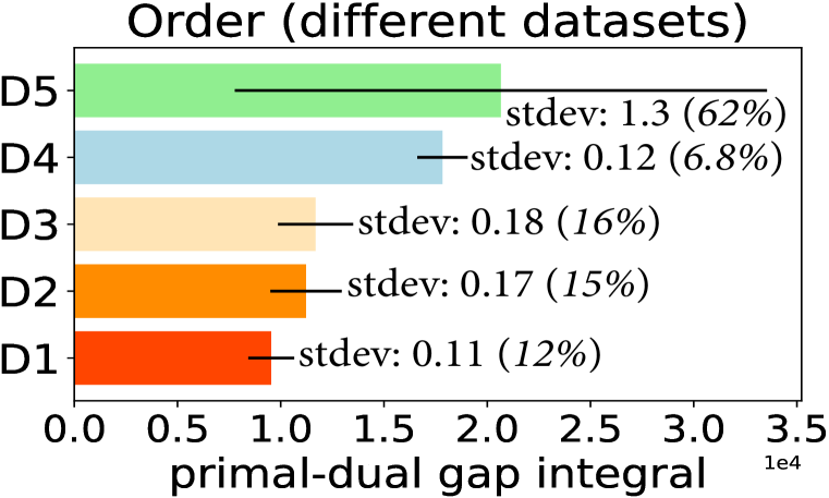
(a) Evaluate RandomAll on five different datasets.

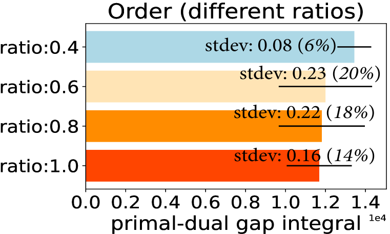
(b) Evaluate RandomNv on MIPLIB mixed neos.

Figure 1: We design two cut selection heuristics, namely RandomAll and RandomNV (see Section 3 for details), which both add the same subset of cuts in random order for a given MILP. The results in (a) and (b) show that adding the same selected cuts in different order leads to variable overall solver performance.

3 Motivating Results

We empirically show that the order of selected cuts, i.e., the selected cuts are added to the LP relaxations in this order, significantly impacts the efficiency of solving MILPs. Moreover, we empirically show that the ratio of selected cuts matters significantly when solving MILPs (see Appendix G.1). Please see Appendix D.2 for details of the datasets used in this section.

Order matters. Previous work (Bixby, 1992; Maros, 2002; Li et al., 2022) has shown that the order of constraints for a given linear program (LP) significantly impacts its constructed initial basis, which is important for solving the LP. As a cut is a linear constraint, adding cuts to the LP relaxations is equivalent to adding constraints to the LP relaxations. Therefore, the order of added cuts could have a significant impact on solving the LP relaxations as well, thus being important for solving MILPs. Indeed, our empirical results show that this is the case. (1) We design a RandomAll cut selection rule, which randomly permutes all the candidate cuts, and adds all the cuts to the LP relaxations in the random order. We evaluate RandomAll on five challenging datasets, namely D1, D2, D3, D4, and D5. We use the SCIP 8.0.0 (Bestuzheva et al., 2021) as the backend solver, and evaluate the solver performance by the average PD integral within a time limit. We evaluate RandomAll on each dataset over ten random seeds, and each bar in Figure 1(a) shows the mean and standard deviation (stdev) of its performance on each dataset. As shown in Figure 1(a), the performance of RandomAll on each dataset varies widely with the order of selected cuts. (2) We further design a RandomNV cut selection rule. RandomNV is different from RandomAll in that it selects a given ratio of the candidate cuts rather than all the cuts. RandomNV first scores each cut using the Normalized Violation (Huang et al., 2022) and selects a given ratio of cuts with high scores. It then randomly permutes the selected cuts. Each bar in Figure 1(b) shows the mean and stdev of the performance of RandomNV with a given ratio on the same dataset. Figures 1(a) and 1(b) show that adding the same selected cuts in different order leads to variable solver performance, which demonstrates that the order of selected cuts is important for solving MILPs.

4 Learning Cut Selection via Hierarchical Sequence Model

In the cut selection task, the optimal subsets that should be selected are inaccessible, but one can assess the quality of selected subsets using a solver and provide the feedbacks to learning algorithms. Therefore, we leverage reinforcement learning (RL) to learn cut selection policies. In this section, we provide a detailed description of our proposed RL framework for learning cut selection. First, we present our formulation of the cut selection as a Markov decision process (MDP) (Sutton & Barto, 2018). Then, we present a detailed description of our proposed hierarchical sequence model (HEM). Finally, we derive a hierarchical policy gradient for training HEM efficiently.

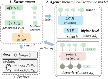
Figure 2: Illustration of our proposed RL framework for learning cut selection policies. We formulate a MILP solver as the environment and the HEM as the agent. Moreover, we train HEM via a hierarchical policy gradient algorithm.

Reinforcement Learning Formulation

As shown in Figure 2, we formulate a MILP solver as the environment and our proposed HEM as the agent. We consider an MDP defined by the tuple $(\mathcal{S},\mathcal{A},r,f)$. Specifically, we specify the state space $\mathcal{S}$, the action space $\mathcal{A}$, the reward function $r:\mathcal{S}\times\mathcal{A}\to\mathbb{R}$, the transition function $f$, and the terminal state in the following. (1) The state space $\mathcal{S}$. Since the current LP relaxation and the generated cuts contain the core information for cut selection, we define a state $s$ by $(M_{\text{LP}},\mathcal{C},\textbf{x}_{\text{LP}}^{*})$. Here $M_{\text{LP}}$ denotes the mathematical model of the current LP relaxation, $\mathcal{C}$ denotes the set of the candidate cuts, and $\textbf{x}_{\text{LP}}^{*}$ denotes the optimal solution of the LP relaxation. To encode the state information, we follow Achterberg (2007); Huang et al. (2022) to design thirteen features for each candidate cut based on the information of $(M_{\text{LP}},\mathcal{C},\textbf{x}_{\text{LP}}^{*})$. That is, we actually represent a state $s$ by a sequence of thirteen-dimensional feature vectors. We present details of the designed features in Appendix F.1. (2) The action space $\mathcal{A}$. To take into account the ratio and order of selected cuts, we define the action space by all the ordered subsets of the candidate cuts $\mathcal{C}$. It can be challenging to explore the action space efficiently, as the cardinality of the action space can be extremely large due to its combinatorial structure. (3) The reward function $r$. To evaluate the impact of the added cuts on solving MILPs, we design the reward function by (i) measures collected at the end of solving LP relaxations such as the dual bound improvement, (ii) or end-of-run statistics, such as the solving time and the primal-dual gap integral. For the first, the reward $r(s,a)$ can be defined as the negative dual bound improvement at each step. For the second, the reward $r(s,a)$ can be defined as zero except for the last step $(s_{T},a_{T})$ in a trajectory, i.e., $r(s_{T},a_{T})$ is defined by the negative solving time or the negative primal-dual gap integral. (4) The transition function $f$. The transition function maps the current state $s$ and the action $a$ to the next state $s^{\prime}$, where $s^{\prime}$ represents the next LP relaxation generated by adding the selected cuts at the current LP relaxation. (5) The terminal state. There is no standard and unified criterion to determine when to terminate the cut separation procedure (Paulus et al., 2022). Suppose we set the cut separation rounds as $T$, then the solver environment terminates the cut separation after $T$ rounds. Under the multiple rounds setting (i.e., $T>1$), we formulate the cut selection as a Markov decision process. Under the one round setting (i.e., $T=1$), the formulation can be simplified as a contextual bandit.

Hierarchical Sequence Model

Motivation. Let $\pi$ denote the cut selection policy $\pi:\mathcal{S}\to\mathcal{P}(\mathcal{A})$, where $\mathcal{P}(\mathcal{A})$ denotes the probability distribution over the action space, and $\pi(\cdot|s)$ denotes the probability distribution over the action space given the state $s$. We emphasize that learning such policies can tackle (P1)-(P3) in cut selection simultaneously. However, directly learning such policies is challenging for the following reasons. First, it is challenging to explore the action space efficiently, as the cardinality of the action space can be extremely large due to its combinatorial structure. Second, the length and max length of actions (i.e., ordered subsets) are variable across different MILPs. However, traditional RL usually deals with problems whose actions have a fixed length. Instead of directly learning the aforementioned policy, many existing learning-based methods (Tang et al., 2020; Huang et al., 2022; Paulus et al., 2022) learn a scoring function that outputs a score given a cut, and select a fixed ratio/number of cuts with high scores. However, they suffer from two limitations as mentioned in Section 1.

Policy network architecture. To tackle the aforementioned problems, we propose a novel hierarchical sequence model (HEM) to learn cut selection policies. To promote efficient exploration, HEM leverages the hierarchical structure of the cut selection task to decompose the policy into two sub-policies, i.e., a higher-level policy $\pi^{h}$ and a lower-level policy $\pi^{l}$. The policy network architecture of HEM is also illustrated in Figure 2. First, the higher-level policy learns the number of cuts that should be selected by predicting a proper ratio. Suppose the length of the state is $N$ and the predicted ratio is $k$, then the predicted number of cuts that should be selected is $\lfloor N*k\rfloor$, where $\lfloor\cdot\rfloor$ denotes the floor function. We define the higher-level policy by $\pi^{h}:\mathcal{S}\to\mathcal{P}(\left[0,1\right])$, where $\pi^{h}(\cdot|s)$ denotes the probability distribution over $\left[0,1\right]$ given the state $s$. Second, the lower-level policy learns to select an ordered subset with the size determined by the higher-level policy. We define the lower-level policy by $\pi^{l}:\mathcal{S}\times\left[0,1\right]\to\mathcal{P}(\mathcal{A})$, where $\pi^{l}(\cdot|s,k)$ denotes the probability distribution over the action space given the state $s$ and the ratio $k$. Specifically, we formulate the lower-level policy as a sequence model, which can capture the interaction among cuts. Finally, we derive the cut selection policy via the law of total probability, i.e., $\pi(a_{k}|s)=\mathbb{E}_{k\sim\pi^{h}(\cdot|s)}[\pi^{l}(a_{k}|s,k)],$ where $k$ denotes the given ratio and $a_{k}$ denotes the action. The policy is computed by an expectation, as $a_{k}$ cannot determine the ratio $k$. For example, suppose that $N=100$ and the length of $a_{k}$ is $10$, then the ratio $k$ can be any number in the interval $[0.1,0.11)$. Actually, we sample an action from the policy $\pi$ by first sampling a ratio $k$ from $\pi^{h}$ and then sampling an action from $\pi^{l}$ given the ratio.

For the higher-level policy, we first model the higher-level policy as a tanh-Gaussian, i.e., a Gaussian distribution with an invertible squashing function ($\tanh$), which is commonly used in deep reinforcement learning (Schulman et al., 2017; Haarnoja et al., 2018). The mean and variance of the Gaussian are given by neural networks. The support of the tanh-Gaussian is $[-1,1]$, but a ratio of selected cuts should belong to $[0,1]$. Thus, we further perform a linear transformation on the tanh-Gaussian. Specifically, we define the parameterized higher-level policy by $\pi^{h}_{\theta_{1}}(\cdot|s)=0.5*\tanh{(K)}+0.5$, where $K\sim\mathcal{N}(\mu_{\theta_{1}}(s),\sigma_{\theta_{1}}(s))$. Since the sequence lengths of states are variable across different instances (MILPs), we use a long-short term memory (LSTM) (Hochreiter & Schmidhuber, 1997) network to embed the sequence of candidate cuts. We then use a multi-layer perceptron (MLP) (Goodfellow et al., 2016) to predict the mean and variance from the last hidden state of the LSTM.

For the lower-level policy, we formulate it as a sequence model. That is, its input is a sequence of candidate cuts, and its output is the probability distribution over ordered subsets of candidate cuts with the size determined by the higher-level policy. Specifically, given a state action pair $(s,k,a_{k})$, the sequence model computes the conditional probability $\pi^{l}_{\theta_{2}}(a_{k}|s,k)$ using a parametric model to estimate the terms of the probability chain rule, i.e., $\pi^{l}_{\theta_{2}}(a_{k}|s,k)=\prod_{i=1}^{m}p_{\theta_{2}}(a_{k}^{i}|a_{k}^{1},\dots,a_{k}^{i-1},s,k)$. Here $s=\{s^{1},\dots,s^{N}\}$ is the input sequence, $m=\lfloor N*k\rfloor$ is the length of the output sequence, and $a_{k}=\{a_{k}^{1},\dots,a_{k}^{m}\}$ is a sequence of $m$ indices, each corresponding a position in the input sequence $s$. Such policy can be parametrized by the vanilla sequence model commonly used in machine translation (Sutskever et al., 2014; Vaswani et al., 2017). However, the vanilla sequence model can only be applied to learning on a single instance, as the number of candidate cuts varies on different instances. To generalize across different instances, we use a pointer network (Vinyals et al., 2015; Bello* et al., 2017)—which uses attention as a pointer to select a member of the input sequence as the output at each decoder step—to parametrize $\pi^{l}_{\theta_{2}}$ (see Appendix F.4.1 for details). To the best of our knowledge, we are the first to formulate the cut selection task as a sequence to sequence learning problem and apply the pointer network to cut selection. This leads to two major advantages: (1) capturing the underlying order information, (2) and the interaction among cuts. This is also illustrated through an example in Appendix E.

Training: hierarchical policy gradient

For the cut selection task, we aim to find $\theta$ that maximizes the expected reward over all trajectories

$$J(\theta)=\mathbb{E}_{s\sim\mu,a_{k}\sim\pi_{\theta}(\cdot|s)}[r(s,a_{k})],$$ (3)

where $\theta=\left[\theta_{1},\theta_{2}\right]$ with $\left[\theta_{1},\theta_{2}\right]$ denoting the concatenation of the two vectors, $\pi_{\theta}(a_{k}|s)=\mathbb{E}_{k\sim\pi^{h}_{\theta_{1}}(\cdot|s)}[\pi^{l}_{\theta_{2}}(a_{k}|s,k)]$, and $\mu$ denotes the initial state distribution.

To train the policy with a hierarchical structure, we derive a hierarchical policy gradient following the well-known policy gradient theorem (Sutton et al., 1999a; Sutton & Barto, 2018).

Proposition 1.

Given the cut selection policy $\pi_{\theta}(a_{k}|s)=\mathbb{E}_{k\sim\pi^{h}_{\theta_{1}}(\cdot|s)}[\pi^{l}_{\theta_{2}}(a_{k}|s,k)]$ and the training objective (3), the hierarchical policy gradient takes the form of

$$\nabla_{\theta_{1}}J(\left[\theta_{1},\theta_{2}\right]) =\mathbb{E}_{s\sim\mu,k\sim\pi^{h}_{\theta_{1}}(\cdot|s)}[\nabla_{\theta_{1}}\log(\pi^{h}_{\theta_{1}}(k|s))\mathbb{E}_{a_{k}\sim\pi^{l}_{\theta 2}(\cdot|s,k)}[r(s,a_{k})]],$$

$$\nabla_{\theta_{2}}J(\left[\theta_{1},\theta_{2}\right]) =\mathbb{E}_{s\sim\mu,k\sim\pi^{h}_{\theta_{1}}(\cdot|s),a_{k}\sim\pi^{l}_{\theta_{2}}(\cdot|s,k)}[\nabla_{\theta_{2}}\log\pi^{l}_{\theta_{2}}(a_{k}|s,k)r(s,a_{k})].$$

We provide detailed proof in Appendix A. We use the derived hierarchical policy gradient to update the parameters of the higher-level and lower-level policies. We implement the training algorithm in a parallel manner that is closely related to the asynchronous advantage actor-critic (A3C) (Mnih et al., 2016). Due to limited space, we summarize the procedure of the training algorithm in Appendix F.3.6. Moreover, we discuss some more advantages of HEM (see Appendix F.4.3 for details). (1) HEM leverages the hierarchical structure of the cut selection task, which is important for efficient exploration in complex decision-making tasks (Sutton et al., 1999b). (2) We train HEM via gradient-based algorithms, which is sample efficient (Sutton & Barto, 2018).

5 Experiments

Our experiments have five main parts: Experiment 1. Evaluate our approach on three classical MILP problems and six challenging MILP problem benchmarks from diverse application areas. Experiment 2. Perform carefully designed ablation studies to provide further insight into HEM. Experiment 3. Test whether HEM can generalize to instances significantly larger than those seen during training. Experiment 4. Visualize the cuts selected by our method compared to the baselines. Experiment 5. Deploy our approach to real-world production planning problems.

Benchmarks. We evaluate our approach on nine $\mathcal{NP}$-hard MILP problem benchmarks, which consist of three classical synthetic MILP problems and six challenging MILP problems from diverse application areas. We divide the nine problem benchmarks into three categories according to the difficulty of solving them using the SCIP 8.0.0 solver (Bestuzheva et al., 2021). We call the three categories easy, medium, and hard datasets, respectively. (1) Easy datasets comprise three widely used synthetic MILP problem benchmarks: Set Covering (Balas & Ho, 1980), Maximum Independent Set (Bergman et al., 2016), and Multiple Knapsack (Scavuzzo et al., 2022). We artificially generate instances following Gasse et al. (2019); Sun et al. (2020). (2) Medium datasets comprise MIK (Atamtürk, 2003) and CORLAT (Gomes et al., 2008), which are widely used benchmarks for evaluating MILP solvers (He et al., 2014; Nair et al., 2020). (3) Hard datasets include the Load Balancing problem, inspired by real-life applications of large-scale systems, and the Anonymous problem, inspired by a large-scale industrial application (Bowly et al., 2021). Moreover, hard datasets contain benchmarks from MIPLIB 2017 (MIPLIB) (Gleixner et al., 2021). Although Turner et al. (2022) has shown that directly learning over the full MIPLIB can be extremely challenging, we propose to learn over subsets of MIPLIB. We construct two subsets, called MIPLIB mixed neos and MIPLIB mixed supportcase. Due to limited space, please see Appendix D.1 for details of these datasets.

Table 1: Policy evaluation on the easy, medium, and hard datasets. The best performance is marked in bold. Let $m$ denote the average number of constraints and $n$ denote the average number of variables. We report the arithmetic mean (standard deviation) of the Time and PD integral.

	Easy: Set Covering ($n=1000,\,\,m=500$)			Easy: Maximum Independent Set ($n=500,\,\,m=1953$)			Easy: Multiple Knapsack ($n=720,\,\,m=72$)
Method	Time(s) $\downarrow$	Improvement (Time, %) $\uparrow$	PD integral $\downarrow$	Time(s) $\downarrow$	Improvement (Time, %) $\uparrow$	PD integral $\downarrow$	Time(s) $\downarrow$	Improvement (Time, %) $\uparrow$	PD integral $\downarrow$
NoCuts	6.31 (4.61)	NA	56.99 (38.89)	8.78 (6.66)	NA	71.31 (51.74)	9.88 (22.24)	NA	16.41 (14.16)
Default	4.41 (5.12)	29.90	55.63 (42.21)	3.88 (5.04)	55.80	29.44 (35.27)	9.90 (22.24)	-0.20	16.46 (14.25)
Random	5.74 (5.19)	8.90	67.08 (46.58)	6.50 (7.09)	26.00	52.46 (53.10)	13.10 (35.51)	-32.60	20.00 (25.14)
NV	9.86 (5.43)	-56.50	99.77 (53.12)	7.84 (5.54)	10.70	61.60 (43.95)	13.04 (36.91)	-32.00	21.75 (24.71)
Eff	9.65 (5.45)	-53.20	95.66 (51.71)	7.80 (5.11)	11.10	61.04 (41.88)	9.99 (19.02)	-1.10	20.49 (22.11)
SBP	1.91 (0.36)	69.60	38.96 (8.66)	2.43 (5.55)	72.30	21.99 (40.86)	7.74 (12.36)	21.60	16.45 (16.62)
HEM (Ours)	1.85 (0.31)	70.60	37.92 (8.46)	1.76 (3.69)	80.00	16.01 (26.21)	6.13 (9.61)	38.00	13.63 (9.63)

	Medium: MIK ($n=413,\,\,m=346$)			Medium: Corlat ($n=466,\,\,m=486$)			Hard: Load Balancing ($n=61000,\,\,m=64304$)
Method	Time(s) $\downarrow$	PD integral $\downarrow$	Improvement $\uparrow$ (PD integral, %)	Time(s) $\downarrow$	PD integral $\downarrow$	Improvement $\uparrow$ (PD integral, %)	Time(s) $\downarrow$	PD integral $\downarrow$	Improvement $\uparrow$ (PD integral, %)
NoCuts	300.01 (0.009)	2355.87 (996.08)	NA	103.30 (128.14)	2818.40 (5908.31)	NA	300.00 (0.12)	14853.77 (951.42)	NA
Default	179.62 (122.36)	844.40 (924.30)	64.10	75.20 (120.30)	2412.09 (5892.88)	14.40	300.00 (0.06)	9589.19 (1012.95)	35.40
Random	289.86 (28.90)	2036.80 (933.17)	13.50	84.18 (124.34)	2501.98 (6031.43)	11.20	300.00 (0.09)	13621.20 (1162.02)	8.30
NV	299.76 (1.32)	2542.67 ( 529.49)	-7.90	90.26 (128.33)	3075.70 (7029.55)	-9.10	300.00 (0.05)	13933.88 (971.10)	6.20
Eff	298.48 (5.84)	2416.57 (642.41)	-2.60	104.38 (131.61)	3155.03 (7039.99)	-11.90	300.00 (0.07)	13913.07 (969.95)	6.30
SBP	286.07 (41.81)	2053.30 (740.11)	12.80	70.41 (122.17)	2023.87 (5085.96)	28.20	300.00 (0.10)	12535.30 (741.43)	15.60
HEM (Ours)	176.12 (125.18)	785.04 (790.38)	66.70	58.31 (110.51)	1079.99 (2653.14)	61.68	300.00 (0.04)	9496.42 (1018.35)	36.10

	Hard: Anonymous ($n=37881,\,\,m=49603$)			Hard: MIPLIB mixed neos ($n=6958,\,\,m=5660$)			Hard: MIPLIB mixed supportcase ($n=19766,\,\,m=19910$)
Method	Time(s) $\downarrow$	PD integral $\downarrow$	Improvement $\uparrow$ (PD integral, %)	Time(s) $\downarrow$	PD integral $\downarrow$	Improvement $\uparrow$ (PD integral, %)	Time(s) $\downarrow$	PD integral $\downarrow$	Improvement $\uparrow$ (PD integral, %)
NoCuts	246.22 (94.90)	18297.30 (9769.42)	NA	253.65 (80.29)	14652.29 (12523.37)	NA	170.00 (131.60)	9927.96 (11334.07)	NA
Default	244.02 (97.72)	17407.01 (9736.19)	4.90	256.58 (76.05)	14444.05 (12347.09)	1.42	164.61 (135.82)	9672.34 (10668.24)	2.57
Random	243.49 (98.21)	16850.89 (10227.87)	7.80	255.88 (76.65)	14006.48 (12698.76)	4.41	165.88 (134.40)	10034.70 (11052.73)	-1.07
NV	242.01 (98.68)	16873.66 (9711.16)	7.80	263.81 (64.10)	14379.05 (12306.35)	1.86	161.67 (131.43)	8967.00 (9690.30)	9.68
Eff	244.94 (93.47)	17137.87 (9456.34)	6.30	260.53 (68.54)	14021.74 (12859.41)	4.30	167.35 (134.99)	9941.55 (10943.48)	-0.14
SBP	245.71 (92.46)	18188.63 (9651.85)	0.59	256.48 (78.59)	13531.00 (12898.22)	7.65	165.61 (135.25)	7408.65 (7903.47)	25.37
HEM (Ours)	241.68 (97.23)	16077.15 (9108.21)	12.10	248.66 (89.46)	8678.76 (12337.00)	40.77	162.96 (138.21)	6874.80 (6729.97)	30.75

Experimental setup. Throughout all experiments, we use SCIP 8.0.0 (Bestuzheva et al., 2021) as the backend solver, which is the state-of-the-art open source solver, and is widely used in research of machine learning for combinatorial optimization (Gasse et al., 2019; Huang et al., 2022; Turner et al., 2022; Nair et al., 2020). Following Gasse et al. (2019); Huang et al. (2022); Paulus et al. (2022), we only allow cutting plane generation and selection at the root node, and set the cut separation rounds as one. We keep all the other SCIP parameters to default so as to make comparisons as fair and reproducible as possible. We emphasize that all of the SCIP solver’s advanced features, such as presolve and heuristics, are open, which ensures that our setup is consistent with the practice setting. Throughout all experiments, we set the solving time limit as 300 seconds. For completeness, we also evaluate HEM with a much longer time limit of three hours. The results are given in Appendix G.6. We train HEM with ADAM (Kingma & Ba, 2014) using the PyTorch (Paszke et al., 2019). Additionally, we also provide another implementation using the MindSpore (Chen, 2021). For simplicity, we split each dataset into the train and test sets with $80\%$ and $20\%$ instances. To further improve HEM, one can construct a valid set for hyperparameters tuning. We train our model on the train set, and select the best model on the train set to evaluate on the test set. Please refer to Appendix F.3 for implementation details, hyperparameters, and hardware specification.

Baselines. Our baselines include five widely used human-designed cut selection rules and a state-of-the-art (SOTA) learning-based method. Cut selection rules include NoCuts, Random, Normalized Violation (NV), Efficacy (Eff), and Default. NoCuts does not add any cuts. Default denotes the default cut selection rule used in SCIP 8.0.0. For learning-based methods, we implement a slight variant of the SOTA learning-based methods (Tang et al., 2020; Huang et al., 2022), namely score-based policy (SBP). Please see Appendix F.2 for implementation details of these baselines.

Evaluation metrics. We use two widely used evaluation metrics, i.e., the average solving time (Time, lower is better), and the average primal-dual gap integral (PD integral, lower is better). Additionally, we provide more results in terms of another two metrics, i.e., the average number of nodes and the average primal-dual gap, in Appendix G.2. Furthermore, to evaluate different cut selection methods compared to pure branch-and-bound without cutting plane separation, we propose an Improvement metric. Specifically, we define the metric by $\text{Im}_{M}(\cdot)=\frac{M(\text{NoCuts})-M(\cdot)}{M(\text{NoCuts})},$ where $M(\text{NoCuts})$ represents the performance of NoCuts, and $M(\cdot)$ represents a mapping from a method to its performance. The improvement metric represents the improvement of a given method compared to NoCuts. We mainly focus on the Time metric on the easy datasets, as the solver can solve all instances to optimality within the given time limit. However, HEM and the baselines cannot solve all instances to optimality within the time limit on the medium and hard datasets. As a result, the average solving time of those unsolved instances is the same, which makes it difficult to distinguish the performance of different cut selection methods using the Time metric. Therefore, we mainly focus on the PD integral metric on the medium and hard datasets. The PD integral is also a well-recognized metric for evaluating the solver performance (Bowly et al., 2021; Cao et al., 2022).

Experiment 1. Comparative evaluation The results in Table 1 suggest the following. (1) Easy datasets. HEM significantly outperforms all the baselines on the easy datasets, especially on Maximum Independent Set and Multiple Knapsack. SBP achieves much better performance than all the rule-based baselines, demonstrating that our implemented SBP is a strong baseline. Compared to SBP, HEM improves the Time by up to $16.4\%$ on the three datasets, demonstrating the superiority of our method over the SOTA learning-based method. (2) Medium datasets. On MIK and CORLAT, HEM still outperforms all the baselines. Especially on CORLAT, HEM achieves at least $33.48\%$ improvement in terms of the PD integral compared to the baselines. (3) Hard datasets. HEM significantly outperforms the baselines in terms of the PD integral on several problems in the hard datasets. HEM achieves outstanding performance on two challenging datasets from MIPLIB 2017 and real-world problems (Load Balancing and Anonymous), demonstrating the powerful ability to enhance MILP solvers with HEM in large-scale real-world applications. Moreover, SBP performs extremely poorly on several medium and hard datasets, which implies that it can be difficult to learn good cut selection policies on challenging MILP problems.

Table 2: Comparison between HEM and HEM without the higher-level model.

	Easy: Maximum Independent Set ($n=500,\,\,m=1953$)			Medium: Corlat ($n=466,\,\,m=486$)			Hard: MIPLIB mixed neos ($n=6958,\,\,m=5660$)
Method	Time(s) $\downarrow$	Improvement $\uparrow$ (Time, %)	PD integral $\downarrow$	Time(s) $\downarrow$	PD integral $\downarrow$	Improvement $\uparrow$ (PD integral, %)	Time(s) $\downarrow$	PD integral $\downarrow$	Improvement $\uparrow$ (PD integral, %)
NoCuts	8.78 (6.66)	NA	71.31 (51.74)	103.30 (128.14)	2818.40 (5908.31)	NA	253.65 (80.29)	14652.29 (12523.37)	NA
Default	3.88 (5.04)	55.81	29.44 (35.27)	75.20 (120.30)	2412.09 (5892.88)	14.42	256.58 (76.05)	14444.05 (12347.09)	1.42
SBP	2.43 (5.55)	72.32	21.99 (40.86)	70.41 (122.17)	2023.87 (5085.96)	28.19	256.48 (78.59)	13531.00 (12898.22)	7.65
HEM w/o H	1.88 (4.20)	78.59	16.70 (28.15)	63.14 (115.26)	1939.08 (5484.83)	31.20	249.21 (88.09)	13614.29 (12914.76)	7.08
HEM (Ours)	1.76 (3.69)	79.95	16.01 (26.21)	58.31 (110.51)	1079.99 (2653.14)	61.68	248.66 (89.46)	8678.76 (12337.00)	40.77

Table 3: Comparison between HEM, HEM-ratio, and HEM-ratio-order.

	Easy: Maximum Independent Set ($n=500,\,\,m=1953$)			Medium: Corlat ($n=466,\,\,m=486$)			Hard: MIPLIB mixed neos ($n=6958,\,\,m=5660$)
Method	Time(s) $\downarrow$	Improvement $\uparrow$ (Time, %)	PD integral $\downarrow$	Time(s) $\downarrow$	PD integral $\downarrow$	Improvement $\uparrow$ (PD integral, %)	Time(s) $\downarrow$	PD integral $\downarrow$	Improvement $\uparrow$ (PD integral, %)
NoCuts	8.78 (6.66)	NA	71.31 (51.74)	103.30 (128.14)	2818.40 (5908.31)	NA	253.65 (80.29)	14652.29 (12523.37)	NA
Default	3.88 (5.04)	55.81	29.44 (35.27)	75.20 (120.30)	2412.09 (5892.88)	14.42	256.58 (76.05)	14444.05 (12347.09)	1.42
SBP	2.43 (5.55)	72.32	21.99 (40.86)	70.41 (122.17)	2023.87 (5085.96)	28.19	256.48 (78.59)	13531.00 (12898.22)	7.65
HEM-ratio-order	2.30 (5.18)	73.80	21.19 (38.52)	70.94 (122.93)	1416.66 (3380.10)	49.74	245.99 (93.67)	14026.75 (12683.60)	4.27
HEM-ratio	2.26 (5.06)	74.26	20.82 (37.81)	67.27 (117.01)	1251.60 (2869.87)	55.59	244.87 (95.56)	13659.93 (12900.59)	6.77
HEM (Ours)	1.76 (3.69)	79.95	16.01 (26.21)	58.31 (110.51)	1079.99 (2653.14)	61.68	248.66 (89.46)	8678.76 (12337.00)	40.77

Experiment 2. Ablation study We present ablation studies on Maximum Independent Set (MIS), CORLAT, and MIPLIB mixed neos, which are representative datasets from the easy, medium, and hard datasets. We provide more results on the other datasets in Appendix G.3.

Contribution of each component. We perform ablation studies to understand the contribution of each component in HEM. We report the performance of HEM and HEM without the higher-level model (HEM w/o H) in Table 2. HEM w/o H is essentially a pointer network. Note that it can still implicitly predicts the number of cuts that should be selected by predicting an end token as used in language tasks (Sutskever et al., 2014). Please see Appendix F.4.2 for details. First, the results in Table 2 show that HEM w/o H outperforms all the baselines on MIS and CORLAT, demonstrating the advantages of the lower-level model. Although HEM w/o H outperforms Default on MIPLIB mixed neos, HEM w/o H performs on par with SBP. A possible reason is that it is difficult for HEM w/o H to explore the action space efficiently, and thus HEM w/o H tends to be trapped to the local optimum. Second, the results in Table 2 show that HEM significantly outperforms HEM w/o H and the baselines on the three datasets. The results demonstrate that the higher-level model is important for efficient exploration in complex tasks, thus significantly improving the solving efficiency.

The importance of tackling (P1)-(P3). We perform ablation studies to understand the importance of tackling (P1)-(P3) in cut selection. (1) HEM. HEM tackles (P1)-(P3) in cut selection simultaneously. (2) HEM-ratio. In order not to learn how many cuts should be selected, we remove the higher-level model of HEM and force the lower-level model to select a fixed ratio of cuts. We denote it by HEM-ratio. Note that HEM-ratio is different from HEM w/o H (see Appendix F.4.2). HEM-ratio tackles (P1) and (P3) in cut selection. (3) HEM-ratio-order. To further mute the effect of the order of selected cuts, we reorder the selected cuts given by HEM-ratio with the original index of the generated cuts, which we denote by HEM-ratio-order. HEM-ratio-order mainly tackles (P1) in cut selection. The results in Table 3 suggest the following. HEM-ratio-order significantly outperforms Default and NoCuts, demonstrating that tackling (P1) by data-driven methods is crucial. HEM significantly outperforms HEM-ratio in terms of the PD integral, demonstrating the significance of tackling (P2). HEM-ratio outperforms HEM-ratio-order in terms of the Time and the PD integral, which demonstrates the importance of tackling (P3). Moreover, HEM-ratio and HEM-ratio-order perform better than SBP on MIS and CORLAT, demonstrating the advantages of using the sequence model to learn cut selection over SBP. HEM-ratio and HEM-ratio-order perform on par with SBP on MIPLIB mixed neos. We provide possible reasons in Appendix G.3.1.

Table 4: Left: The generalization ability of HEM. Right: Test on Production Planning problems.

	Maximum Independent Set $(n=1000,\,\,m=3946,\,\,4\times)$			Maximum Independent Set $(n=5940,\,\,m=1500,\,\,9\times)$
Method	Time(s) $\downarrow$	Improvement $\uparrow$ (Time, %)	PD integral $\downarrow$	Time(s) $\downarrow$	Improvement $\uparrow$ (Time, %)	PD integral $\downarrow$
NoCuts	170.06 (100.61)	NA	874.45 (522.29)	300.00 (0)	NA	2019.93 (353.27)
Default	42.40 (76.00)	48.72	198.61 (331.20)	111.18 (144.13)	60.91	616.46 (798.94)
Random	118.25 (109.05)	-43.00	574.33 (516.11)	245.13 (115.80)	13.82	1562.20 (793.09)
NV	160.30 (101.41)	-93.86	784.98 (493.24)	299.97 (0.49)	-5.46	1922.52 (349.67)
Eff	158.75 (100.40)	-91.98	779.63 (493.05)	299.45 (3.77)	-5.28	1921.61 (361.26)
SBP	50.55 (89.14)	38.87	253.81 (426.94)	108.42 (143.68)	61.88	680.41 (903.88)
HEM (Ours)	35.34 (67.91)	57.26	160.56 (282.03)	108.02 (143.02)	62.02	570.48 (760.65)

	Production Planning ($n=3582.25,\,\,m=5040.42$)
Method	Time (s) $\downarrow$	Improvement $\uparrow$ (Time, %)	PD integral $\downarrow$	Improvement $\uparrow$ (PD integral, %)
NoCuts	278.79 (231.02)	NA	17866.01 (21309.85)	NA
Default	296.12 (246.25)	-6.22	17703.39 (21330.40)	0.91
Random	280.18 (237.09)	-0.50	18120.21 (21660.01)	-1.42
NV	259.48 (227.81)	6.93	17295.18 (21860.07)	3.20
Eff	263.60 (229.24)	5.45	16636.52 (21322.89)	6.88
SBP	276.61 (235.84)	0.78	16952.85 (21386.07)	5.11
HEM (Ours)	241.77 (229.97)	13.28	15751.08 (20683.53)	11.84

Experiment 3. Generalization We evaluate the ability of HEM to generalize across different sizes of MILPs. Let $n\times m$ denote the size of MILP instances. Following Gasse et al. (2019); Sun et al. (2020), we test the generalization ability of HEM on Set Covering and Maximum Independent Set (MIS), as we can artificially generate instances with arbitrary sizes for synthetic MILP problems. On MIS, we test HEM on four times and nine times larger instances than those seen during training. The results in Table 4 (Left) show that HEM significantly outperforms the baselines in terms of the Time and the PD integral on $4\times$ and $9\times$ MIS, demonstrating the superiority of HEM in terms of the generalization ability. Interestingly, SBP also generalizes well to large instances, demonstrating that SBP is a strong baseline. We provide more results on Set Covering in Appendix G.4.

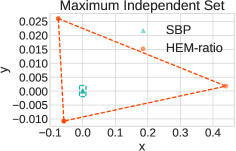
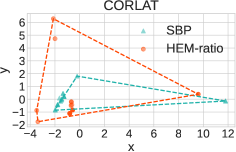
Figure 3: We perform principal component analysis on the cuts selected by HEM-ratio and SBP. Colored points illustrate the reduced cut features. The area covered by the dashed lines represents the diversity of selected cuts. The results show that HEM-ratio selects much more diverse cuts than SBP.

Experiment 4. Visualization of selected cuts We visualize the diversity of selected cuts, an important metric for evaluating whether the selected cuts complement each other nicely (Dey & Molinaro, 2018b). We visualize the cuts selected by HEM-ratio and SBP on a randomly sampled instance from Maximum Independent Set and CORLAT, respectively. We evaluate HEM-ratio rather than HEM, as HEM-ratio selects the same number of cuts as SBP. Furthermore, we perform principal component analysis on the selected cuts to reduce the cut features to two-dimensional space. Colored points illustrate the reduced cut features. To visualize the diversity of selected cuts, we use dashed lines to connect the points with the smallest and largest x,y coordinates. That is, the area covered by the dashed lines represents the diversity. Figure 3 shows that SBP tends to select many similar cuts that are possibly redundant, especially on Maximum Independent Set. In contrast, HEM-ratio selects much more diverse cuts that can well complement each other. Please refer to Appendix G.5 for results on more datasets.

Experiment 5. Deployment in real-world production planning problems To further evaluate the effectiveness of our proposed HEM, we deploy HEM to large-scale real-world production planning problems at an anonymous enterprise, which is one of the largest global commercial technology enterprises. Please refer to Appendix D.3 for more details of the problems. The results in Table 4 (Right) show that HEM significantly outperforms all the baselines in terms of the Time and PD integral. The results demonstrate the strong ability to enhance modern MILP solvers with our proposed HEM in real-world applications. Interestingly, Default performs poorer than NoCuts, which implies that an improper cut selection policy could significantly degrade the performance of MILP solvers.

6 Conclusion

In this paper, we observe from extensive empirical results that the order of selected cuts has a significant impact on the efficiency of solving MILPs. We propose a novel hierarchical sequence model (HEM) to learn cut selection policies via reinforcement learning. Specifically, HEM consists of a two-level model: (1) a higher-level model to learn the number of cuts that should be selected, (2) and a lower-level model—that formulates the cut selection task as a sequence to sequence learning problem—to learn policies selecting an ordered subset with the size determined by the higher-level model. Experiments show that HEM significantly improves the efficiency of solving MILPs compared to human-designed and learning-based baselines on both synthetic and large-scale real-world MILPs. We believe that our proposed approach brings new insights into learning cut selection.

7 Ethics Statement

As our work is fundamental research in solving mixed-integer linear programs (MILPs), there are no direct ethical risks. Modern MILP solvers with expert-designed cut selection heuristics aim to solve general MILPs, while modern MILP solvers with our proposed HEM can learn more effective cut selection heuristics from MILPs collected from certain types of real-world applications.

8 Reproducibility Statement

To ensure reproducibility, we describe our proposed HEM in Section 4 and provide more implementation details in Appendix F. Moreover, we provide the pseudocode of our proposed HEM in Appendix F.3.6. We will release all the source codes publicly once the paper is accepted.

All datasets except the real-world production planning problems used in the experiments are publicly available. Please refer to Appendix D for details of these datasets. We will also publicly release the dataset from the real-world production planning problems once the paper is accepted.

Appendix A Proof

A.1 Proof of Proposition 1

Proof.

The optimization objective takes the form of

$$J(\theta) =\mathbb{E}_{s\sim\mu,a_{k}\sim\pi_{\theta}(\cdot|s)}[r(s,a_{k})]$$

$$=\mathbb{E}_{s\sim\mu}[\sum_{a_{k}}\int_{k=0}^{1}\pi^{h}_{\theta_{1}}(k|s)\pi^{l}_{\theta_{2}}(a_{k}|s,k)r(s,a_{k})dk]$$

$$=\mathbb{E}_{s\sim\mu}[\int_{k=0}^{1}\sum_{a_{k}}\pi^{h}_{\theta_{1}}(k|s)\pi^{l}_{\theta_{2}}(a_{k}|s,k)r(s,a_{k})dk],$$

where $\theta=\left[\theta_{1},\theta_{2}\right]$ with $\left[\theta_{1},\theta_{2}\right]$ denoting the concatenation of the two vectors, $\pi_{\theta}(a_{k}|s)=\mathbb{E}_{k\sim\pi^{h}_{\theta_{1}}(\cdot|s)}[\pi^{h}_{\theta_{2}}(a_{k}|s,k)]$, and $\mu$ denotes the initial state distribution.

We first compute the policy gradient for $\theta_{1}$:

$$\nabla_{\theta_{1}}J(\left[\theta_{1},\theta_{2}\right])$$

$$= \nabla_{\theta_{1}}(\mathbb{E}_{s\sim\mu}[\int_{k=0}^{1}\sum_{a_{k}}\pi^{h}_{\theta_{1}}(k|s)\pi^{l}_{\theta_{2}}(a_{k}|s,k)r(s,a_{k})dk])$$

$$= \mathbb{E}_{s\sim\mu}[\nabla_{\theta_{1}}[\int_{k=0}^{1}\pi_{\theta_{1}}^{h}(k|s)\sum_{a_{k}}\pi_{\theta_{2}}^{l}(a_{k}|s,k)r(s,a_{k})dk]].$$

Let

$$r^{h}(s,k,\theta_{2}) =\sum_{a_{k}}\pi_{\theta_{2}}^{l}(a_{k}|s,k)r(s,a_{k})$$

$$=\mathbb{E}_{a_{k}\sim\pi_{\theta_{2}}^{l}(\cdot|s,k)}[r(s,a_{k})],$$

then we have that

$$\nabla_{\theta_{1}}J(\left[\theta_{1},\theta_{2}\right]) =\mathbb{E}_{s\sim\mu}[\nabla_{\theta_{1}}[\int_{k=0}^{1}\pi_{\theta_{1}}^{h}(k|s)r(s,k,\theta_{2})dk]]$$

$$=\mathbb{E}_{s\sim\mu,k\sim\pi_{\theta_{1}}^{h}(\cdot|s)}[\nabla_{\theta_{1}}\log\pi_{\theta_{1}}^{h}(k|s)r(s,k,\theta_{2})].$$

Therefore, we have that

$$\nabla_{\theta_{1}}J(\left[\theta_{1},\theta_{2}\right])$$

$$=\mathbb{E}_{s\sim\mu,k\sim\pi^{h}_{\theta_{1}}(\cdot|s)}[\nabla_{\theta_{1}}\log(\pi^{h}_{\theta_{1}}(k|s))\mathbb{E}_{a_{k}\sim\pi^{l}_{\theta_{2}}(\cdot|s,k)}[r(s,a_{k})]].$$

We then compute the policy gradient for $\theta_{2}$:

$$\nabla_{\theta_{2}}J(\left[\theta_{1},\theta_{2}\right])$$

$$= \nabla_{\theta_{2}}(\mathbb{E}_{s\sim\mu}[\int_{k=0}^{1}\sum_{a_{k}}\pi^{h}_{\theta_{1}}(k|s)\pi^{l}_{\theta_{2}}(a_{k}|s,k)r(s,a_{k})dk])$$

$$= \mathbb{E}_{s\sim\mu,k\sim\pi_{\theta_{1}}^{h}(\cdot|s)}[\nabla_{\theta_{2}}[\sum_{a_{k}}\pi_{\theta_{2}}^{l}(a_{k}|s,k)r(s,a_{k})]]$$

$$= \mathbb{E}_{s\sim\mu,k\sim\pi_{\theta_{1}}^{h}(\cdot|s),a_{k}\sim\pi_{\theta_{2}}^{l}(\cdot|s,k)}[\nabla_{\theta_{2}}\log\pi_{\theta_{2}}^{l}(a_{k}|s,k)r(s,a_{k})],$$

which completes the proof. ∎

Appendix B Related Work

Machine learning for MILP. The use of machine learning methods to help improve the MILP solver performance has been an active topic of significant interest in recent years (Bengio et al., 2021; Lodi & Zarpellon, 2017; Bowly et al., 2021; Gasse et al., 2019). During the solving process of the solvers, many crucial decisions that significantly impact the solver performance are based on heuristics (Achterberg, 2007). Recent methods propose to replace these hand-crafted heuristics with machine learning models (Bengio et al., 2021). This line of research has shown significant improvement on the solver performance, including cut selection (Tang et al., 2020; Paulus et al., 2022; Turner et al., 2022; Baltean-Lugojan et al., 2019), variable selection (Khalil et al., 2016; Gasse et al., 2019; Balcan et al., 2018; Zarpellon et al., 2021), node selection (He et al., 2014; Sabharwal et al., 2012), column generation (Morabit et al., 2021), and primal heuristics selection (Khalil et al., 2017; Hendel et al., 2019). In this paper, we focus on cut selection, which plays a significant role in modern MILP solvers (Dey & Molinaro, 2018a; Tang et al., 2020).

For cut selection, many existing learning-based methods (Tang et al., 2020; Paulus et al., 2022; Huang et al., 2022) focus on learning which cuts should be preferred by learning a scoring function to measure cut quality. Specifically, (Tang et al., 2020) proposes a reinforcement learning approach to learn to score Gomory cuts (Gomory, 1960) and select a Gomory cut with the best scores. Furthermore, (Paulus et al., 2022) designs a lookahead selection rule which selects a cut that yields the best dual bound improvement, and proposes to learn the expert rule via imitation learning. Instead of selecting the best cut, (Huang et al., 2022) frames cut selection as multiple instance learning to learn a scoring function and selects a fixed ratio of cuts with high scores. However, they neglect the importance of learning how many cuts should be selected. Moreover, we empirically show that the order of selected cuts has a large impact on the efficiency of solving MILPs (see Section 3).

Moreover, (Turner et al., 2022) proposes to learn the weightings of four existing scoring rules designed by experts. For the theoretical analysis, (Balcan et al., 2021) provides some provable guarantees for learning cut selection policies.

Sequence model. Sequence model such as long-short term memory and Transformer has achieved outstanding performance in language tasks such as machine translation (Hochreiter & Schmidhuber, 1997; Sutskever et al., 2014; Vaswani et al., 2017). For combinatorial optimization, recent works (Vinyals et al., 2015; Bello* et al., 2017) propose a variant of the traditional sequence model, namely pointer network, which is applied to directly finding solutions for specific combinatorial optimization problems, such as the Travelling Salesman Problem (Lenstra & Shmoys, 2009). Instead of finding solutions directly, we propose to use the pointer network for cut selection in modern MILP solvers. To the best of our knowledge, we are the first to apply the pointer network to cut selection, which not only captures the order of selected cuts, but also can well capture the interaction among cuts to select cuts that complement each other nicely.

Appendix C More Details of Background

C.1 More details of the primal-dual gap integral

We keep track of two important bounds when running branch-and-cut, including the global primal and dual bound. The global primal bound corresponds to the value of the best feasible solution found so far, which is the best upper bound of the problem in (1). The global dual bound corresponds to the minimum dual bound across all leaves of the search tree, which is the best lower bound of the problem in (1). We define the primal-dual gap integral by the area between the curve of the solver’s global primal bound and the curve of the solver’s global dual bound. With a time limit $T$, we define the primal-dual gap integral by

$$\int_{t=0}^{T}(\textbf{c}^{T}\textbf{x}_{t}^{*}-\textbf{z}_{t}^{*})\mathrm{d}t,$$

where c is the objective coefficient vector as in (1), $\textbf{x}_{t}^{*}$ is the best feasible solution found at time $t$, $\textbf{z}_{t}^{*}$ is the best dual bound at time $t$. We define the primal-dual gap by the difference between the global primal bound and the global dual bound. In SCIP 8.0.0 (Bestuzheva et al., 2021), the initial value of the primal-dual gap is set to a constant 100. The primal-dual gap integral is a well-recognized metric for evaluating solver performance. For example, the primal-dual gal integral is a primary evaluation metric in the NeurIPS 2021 ML4CO competition (Bowly et al., 2021).

Appendix D Details of the Datasets Used in this Paper

D.1 The datasets used in the main evaluation

Algorithm 1 Pseudo code for constructing MIPLIB datasets

1:  Input the initial instance $I_{0}$, the set of full MIPLIB $\mathcal{M}$, an empty set $\mathcal{M}^{\prime}$, an empty queue $Q$.

2:  Initialize $Q$ with the instance $I_{0}$, $I_{0}\to Q$

3:  while Q is not empty do

4:     n$=$Q.size()

5:     for $i=1,\dots,n$ do

6:        Pull an element from $Q$, namely $I^{\prime}$

7:        Compute the similarity scores between each instance in $\mathcal{M}$ except $I^{\prime}$ and $I^{\prime}$

8:        Select five instances with the best similarity scores $\mathcal{M}_{i}$

9:        for $I$ in $\mathcal{M}_{i}$ do

10:           if $I$ not in $\mathcal{M}^{\prime}$ then

11:              Push $I$ to $\mathcal{M}^{\prime}$; Push $I$ to $Q$

12:           end if

13:        end for

14:     end for

15:  end while

16:  Return $\mathcal{M}^{\prime}$

Easy datasets. The SCIP 8.0.0 solver needs one minute to solve the MILP instances in the easy datasets to optimality. Easy datasets are comprised of three synthetic MILP problems: Set Covering (Balas & Ho, 1980), Maximum Independent Set (Bergman et al., 2016), and Multiple Knapsack (Scavuzzo et al., 2022). We choose these three classes of problems for the following reasons. First, they are widely used benchmarks for evaluating MILP solvers (Gasse et al., 2019; Huang et al., 2022; Sun et al., 2020; Gupta et al., 2022). Second, they represent a wide collection of MILP problems encountered in practice. Third, for each class of these problems, the average number of generated cuts is at least twenty, which ensures that proper cut selection strategies are significant for improving the solver performance. Similarly to (Gasse et al., 2019; Scavuzzo et al., 2022; Sun et al., 2020; Gupta et al., 2022), we generate set covering instances with 500 rows and 1000 columns, Maximum Independent Set instances with graphs of 500 nodes and affinity set to 4, multiple knapsack instances with 60 items and 12 knapsacks. For each benchmark, we generate a training set of 10,000 instances, and a test set of 100 instances that are never seen during training. Specifically, readers can refer to https://github.com/ds4dm/learn2branch or https://github.com/lascavana/rl2branch for code to generate the easy datasets. We will also release our code once the paper is accepted to be published.

Medium datasets. The SCIP 8.0.0 solver needs at least five minutes to solve the instances in the medium datasets to optimality. Following He et al. (2014); Hutter et al. (2010); Nair et al. (2020), medium datasets comprise MIK (Atamtürk, 2003), a set of MILP problems with knapsack constraints, and CORLAT (Gomes et al., 2008), a real dataset used for the construction of a wildlife corridor for grizzly bears in the Northern Rockies region. Each problem set is split into training and test sets with $80\%$ and $20\%$ of the instances. Readers can refer to https://atamturk.ieor.berkeley.edu/data/mixed.integer.knapsack/ for MIK. Readers can refer to https://bitbucket.org/mlindauer/aclib2/src/master/ for CORLAT.

Table 5: Criteria for removing instances from MIPLIB 2017.

Criteria	$\%$ of instances removed
Tags: feasibility, numerics, infeasible, no solution	$4.5\%$, $17.4\%$, $2.8\%$, $0.9\%$
Presolve longer than 300 seconds under default conditions	$4.8\%$
Solved to optimality at root	$9.9\%$

Hard datasets. The SCIP 8.0.0 solver needs at least one hour to solve the instances in the hard datasets to optimality.

(1) Benchmarks from MIPLIB 2017. Note that MIPLIB 2017 (MIPLIB) (Gleixner et al., 2021) contains instances of MILPs across many different application areas and has been used as a long-standing standard benchmark for MILP solvers (Nair et al., 2020; Turner et al., 2022; Gleixner et al., 2021). Previous work (Turner et al., 2022) has shown that directly learning over the full MIPLIB can be extremely challenging, as these instances are heterogeneous but machine learning has difficulty in learning from heterogeneous datasets. Despite this challenge, we take the first step towards learning over subsets of MIPLIB. Specifically, we construct two subsets by selecting similar instances from MIPLIB. We measure the similarity between instances by 100 human-designed instance features (Gleixner et al., 2021). Following Turner et al. (2022), we first discard instances from MILLIB that satisfy any of the criteria in Table 5. This ensures that a good cut selection policy can significantly improve the dual bound on the remaining instances. Note that we only use three of seven criteria that are used in (Turner et al., 2022) to preserve as many instances as possible.

To select similar instances from MIPLIB 2017, we first choose a representative instance with knapsack constraints (neos-1456979), and a representative instance with set covering constraints (supportcase40). Then we construct the dataset MIPLIB mixed neos following the procedure in Algorithm 1 with the initial instance neos-1456979. We construct the dataset MIPLIB mixed supportcase following the procedure in Algorithm 1 with the initial instance supportcase40. Note that We measure the similarity between instances by 100 human-designed instance features (Gleixner et al., 2021). Each dataset is split into training and test sets with $80\%$ and $20\%$ of the instances.

Specifically, MIPLIB mixed neos contains 20 instances: neos-1456979, ic97_tension, icir97_tension, l2p12, lectsched-4-obj, lectsched-5-obj, loopha13, neos-686190, neos-2294525-abba, neos-3009394-lami, neos-3046601-motu, neos-3046615-murg, neos-3610173-itata, neos-4338804-snowy, neos-5221106-oparau, neos-5260764-orauea, neos-5261882-treska, neos-5266653-tugela, neos16, and timtab1CUTS.

Moreover, MIPLIB mixed supportcase contains 40 instances: supportcase40, 30_70_45_05_100, 30_70_45_095_100, acc-tight2, acc-tight4, acc-tight5, comp07-2idx, comp08-2idx, comp12-2idx, comp21-2idx, decomp1, decomp2, gus-sch, istanbul-no-cutoff, mkc, mkc1, neos-555343, neos-555424, neos-738098, neos-872648, neos-933562, neos-933638, neos-933966, neos-935234, neos-935769, neos-983171, neos-1330346, neos-1337307, neos-1396125, neos-3209462-rhin, neos-3755335-nizao, neos-3759587-noosa, neos-4300652-rahue, neos18, physiciansched6-1, physiciansched6-2, piperout-d27, qiu, reblock354, and supportcase37.

Table 6: The statistical description of used datasets. In all datasets, $m$ denotes the average number of constraints and $n$ denotes the average number of variables. Inference Time denotes the inference time of our proposed HEM given the average number of candidate cuts.

Datasets	Set Covering	Maximum Independent Set	Multiple Knapsack	MIK	CORLAT	Load Balancing	Anonymous	MIPLIB mixed neos	MIPLIB mixed supportcase
$m$	500	1953	72	346	486	64304	49603	5660	19910
$n$	1000	500	720	413	466	61000	37881	6958	19766
Avg. Candidate Cuts	780.51 $\pm$ 289.92	57.04 $\pm$ 15.53	45.00 $\pm$ 12.71	62.00 $\pm$ 13.1	60.00 $\pm$ 33.29	392.53 $\pm$ 32.92	79.40 $\pm$ 72.64	239.00 $\pm$ 154	173.25 $\pm$ 267.27
Inference Time (s)	1.58	0.11	0.09	0.12	0.12	0.77	0.15	0.47	0.34

(2) Benchmarks used in NeurIPS 2021 ML4CO competition The Load Balancing and Anonymous problems used in the main text are from the NeurIPS 2021 ML4CO competition (Bowly et al., 2021). Readers can refer to https://www.ecole.ai/2021/ml4co-competition/ for details of the competition. The competition releases three challenging datasets, but we only use two of the three datasets. The major reason is that the average number of the candidate cuts on the instances from the third dataset (Item Placement) is less than five, which makes cut selection has little impact on the overall solver performance.

D.1.1 Detailed description of the aforementioned datasets

In this part, we provide detailed description of the aforementioned datasets. Note that all datasets we use except MIPLIB 2017 are application-specific, i.e., they contain instances from only a single application. We summarize the statistical description of the used datasets in this paper in Table 6. Let $n,m$ denote the average number of variables and constraints in the MILPs. Let $m\times n$ denote the size of the MILPs. We emphasize that the largest size of our used datasets is up to two orders of magnitude larger than that used in previous learning-based cut selection methods (Tang et al., 2020; Paulus et al., 2022), which demonstrates the superiority of our proposed HEM. Moreover, we test the inference time of our proposed HEM given the average number of candidate cuts. The results in Table 6 show that the computational overhead of the HEM is very low.

D.2 Datasets used in Section 3 in the main text

In Figure 1(a) in the main text, we use five challenging datasets, namely D1, D2, D3, D4, and D5, respectively. Specifically, D1 represents MIPLIB mixed supportcase, D2 represents the single instance neos-1456979 from MIPLIB 2017, D3 represents MIPLIB mixed neos, D4 represents Anonymous, and D5 represents the single instance lectsched-5-obj from MIPLIB 2017. In Figure 1(b) in the main text, we use the dataset MIPLIB mixed neos.

D.3 Large-scale real-world production planning problems

The production planning problem aims to find the optimal production planning for thousands of factories according to the daily order demand. The constraints include the production capacity for each production line in each factory, transportation limit, the order rate, etc. The optimization objective is to minimize the production cost and lead time simultaneously. We split the dataset into training and test sets with $80\%$ and $20\%$ of the instances. The average size of the production planning problems is approximately equal to $3500\times 5000=1.75\times 10^{8}$, which are large-scale real-world problems. To promote the machine learning community for MILP, we will release the dataset once the paper is accepted to be published.

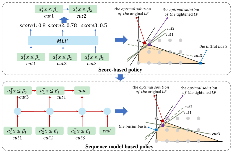
Figure 4: Illustration of selecting cuts using a sequence to sequence model compared to using a scoring function. The sequence model has two main advantages. First, it captures the interaction among cuts by selecting cuts one by one. Consequently, it selects cut3 and cut1 that complement each other nicely, leading to more tightened LP relaxation. Second, it naturally captures the order of selected cuts. Better order of selected cuts may lead to a better initial basis, thus solving the LP relaxation faster (Li et al., 2022) (see Section 3).

Appendix E Illustration of Advantages of Using a Sequence Model

Figure 4 illustrate two major advantages of using the sequence model to learn cut selection. First, the sequence model takes into account the order of selected cuts by modeling the selected cuts as an output sequence. As shown in Figure 4, the order of cuts determined by the sequence model is better than the score-based method, thus leading to a better initial basis for solving the LP relaxation faster. Second, the sequence model captures the interaction among cuts, as it models the joint conditional probability of the selected cuts given an input sequence of the candidate cuts. As shown in Figure 4, the sequence model selects cuts that complement each other nicely, thus leading to a more tightened LP relaxation and speeding up solving the MILP.

Appendix F Algorithm Implementation and Experimental Settings

F.1 Designed cut features

Table 7: The designed cut features of a generated cut $\bm{\alpha}^{T}\textbf{x}\leq\beta$. (Suppose c denotes the objective coefficient.)

Feature	Description	Number
cut coefficients	the mean, max, min, std of cut coefficients	4
objective coefficients	the mean, max, min, std of the objective coefficients	4
parallelism	the parallelism between the objective and the cut $\frac{\textbf{c}^{T}\bm{\alpha}}{|\textbf{c}||\bm{\alpha}|}$	1
efficacy	the Euclidean distance of the cut hyperplane to the current LP solution	1
support	the proportion of non-zero coefficients of the cut	1
integral support	the proportion of non-zero coefficients with respect to integer variables of the cut	1
normalized violation	the violation of the cut to the current LP solution $\max\{0,\frac{\bm{\alpha}^{T}\textbf{x}^{*}_{\text{LP}}-\beta}{|\beta|}\}$	1

Following Huang et al. (2022); Wesselmann & Stuhl (2012); Dey & Molinaro (2018b); Achterberg (2007), we design thirteen cut features for the cut selection task, such as the extent to which a cut is violated by the current LP solution and the proportion of non-zero coefficients of a cut. We present a detailed description of the designed cut features in Table 7. We emphasize that we do not tune the cut features. Therefore, it is promising to further improve our method by designing better cut features or using graph neural networks to learn better features in future work.

F.2 Implementation details of the baselines

In this part, we present a detailed description of all the baselines used in this paper. We denote a cut by $\bm{\alpha}^{T}\textbf{x}\leq\beta$ and the optimal solution of the current LP relaxation by $\textbf{x}^{*}$. Throughout all experiments, we set the ratio of selected cuts as $0.2$ for all score-based rules and learning baselines.

Random. Random selects a fixed ratio of the candidate cuts stochastically. The ratio is set as $0.2$ in this paper.

Normalized Violation (NV). NV is a score-based rule. It scores each cut based on the normalized violation of the cut to the current LP solution, and selects a fixed ratio of cuts with high scores. The normalized violation is defined by $\max\{0,\frac{\bm{\alpha}^{T}\textbf{x}^{*}_{\text{LP}}-\beta}{|\beta|}\}$. The ratio is set as $0.2$ in this paper.

Efficacy (Eff). Eff is a score-based rule. It scores each cut based on the Euclidean distance of the cut hyperplane to the current LP solution, and selects a fixed ratio of cuts with high scores. The ratio is set as $0.2$ in this paper.

Default. Default is the default cut selection rule used in SCIP 8.0.0 (Bestuzheva et al., 2021). Please refer to (Achterberg, 2007) for a detailed description of the SCIP’s default cut selection rule. Note that Default tackles the two problems: (1) which cuts should be preferred, and (2) how many cuts should be selected, in cut selection by human-designed heuristics. That is, Default selects variable ratios of cuts rather than a fixed ratio.

Score-based policy (SBP). Since the state-of-the-art (SOTA) reinforcement learning based method for cut selection (Tang et al., 2020) is designed for the setting that selects the best cut in each round, we implement a slight variant of the SOTA to adapt to our setting that selects a subset of cuts in each round, namely SBP. Specifically, the core idea of SBP is learning a scoring function to measure cut quality as Tang et al. (2020); Huang et al. (2022); Paulus et al. (2022) do. For a fair comparison, SBP uses the same cut features as HEM and we train SBP via reinforcement learning as well. Our implemented SBP is also a slight variant of the method proposed in Huang et al. (2022). We emphasize that experiments in the main text show that our implemented SBP is a strong baseline. Specifically, we implement the scoring function with a multi-layer perceptron that predicts the score of a given cut. That is, the scoring function predicts a cut’s score based on the features of the cut. The MLP network contains two hidden layers with 128 units. Moreover, we train the scoring function via evolutionary strategies as (Tang et al., 2020) does. We will also release the code for implementing SBP once the paper is accepted to be published.

F.3 Implementation details and hyperparameters

F.3.1 Hardware specification

Throughout all experiments, we use a single machine that contains eight GPU devices (NVidia GeForce GTX 3090 Ti) and two Intel Gold 6246R CPUs.

F.3.2 Solver setup

For reproducibility, we emphasize that all results in the main text are obtained by averaging results over the SCIP random seeds $\{1,2,3\}$.

Table 8: Evaluation on real-world production planning problems with rewards being the negative PD integral. The results show that HEM still significantly outperforms all the baselines.

	Production planning
Method	Time (s)	Improvement (Time, %)	PD integral	Improvement (PD integral, %)
NoCuts	278.79	NA	17866.01	NA
Default	296.12	-6.22	17703.39	0.91
Random	280.18	-0.50	18120.21	-1.42
NV	259.48	6.93	17295.18	3.20
Eff	263.60	5.45	16636.52	6.88
SBP	276.61	0.78	16952.85	5.11
HEM (Ours)	251.64	9.74	16533.05	7.46

F.3.3 Reward function

On the easy datasets, we set the reward as the negative solving time. On the medium and hard datasets, we set the reward as the negative primal-dual gap integral within a time limit of 300 seconds.

For the real-world production planning problems, we set the reward as the negative primal-dual gap integral within a time limit of 600 seconds or the negative dual bound improvement. The results reported in the main text are achieved by HEM with the negative dual bound improvement reward. We provide the performance of HEM that uses the negative primal-dual gap integral in Table 8. The results still show that HEM significantly outperforms all the baselines in terms of the Time and PD integral.

We emphasize that we can set the reward according to our objective in real-world problems. For example, suppose we aim to minimize the primal-dual gap within a time limit, then we can set the reward as the primal-dual gap within the time limit.

F.3.4 Policy network architecture

The higher-level model contains an LSTM encoder and an MLP. The LSTM network encodes variable-sized inputs into hidden vectors with dimension 128. The MLP network contains two hidden layers with 128 units. The lower-level model is essentially a pointer network. We keep the hyperparameters of the pointer network as that used in (Bello* et al., 2017).

Algorithm 2 Pseudo code for training the HEM

.

1:  Initialize Hierarchical sequence model $\pi_{[\theta_{1},\theta_{2}]}$, MILP instances $\mathcal{D}$, training dataset $\mathcal{D}_{\text{train}}$, batch size $N_{b}$, training epochs $N_{e}$, policy learning rate $\alpha$

2:  for $N_{e}$ epochs do

3:     Empty the training dataset $\mathcal{D}_{\text{train}}$

4:     for $N_{b}$ steps do

5:        Randomly sample a MILP $s_{0}$ from $\mathcal{D}$

6:        Take action $k$ and $a_{k}$ at state $s_{0}$ with the policy $\pi$

7:        Receive reward $r$ and add $(s_{0},k,a_{k},r)$ to $\mathcal{D}_{\text{train}}$

8:     end for

9:     Compute hierarchical policy gradient using $\mathcal{D}_{\text{train}}$ as in proposition 1

10:     Update the parameters, $\theta_{1}=\theta_{1}+\alpha\nabla_{\theta_{1}}J(\left[\theta_{1},\theta_{2}\right])$, $\theta_{2}=\theta_{2}+\alpha\nabla_{\theta_{2}}J(\left[\theta_{1},\theta_{2}\right])$

11:  end for

F.3.5 Optimization

Throughout all experiments, we apply Adam optimizer with learning rate $\alpha_{1}=1\times 10^{-4}$ to optimize the lower-level model, and learning rate $\alpha_{2}=5\times 10^{-4}$ to optimize the higher-level model. For each epoch, we collect 32 samples for training, and we set the total epochs as 100. It is surprising that learning a good cut selection policy does not need too much data as shown in Tang et al. (2020). For training stability, we delay the higher-level policy update. This creates a two-timescale algorithm, as often required for convergence in the linear setting (Fujimoto et al., 2018; Konda & Tsitsiklis, 2003). We set the delay update freq as two. That is, we first train the lower-level policy twice, then train the higher-level policy once. Additionally, the results in Appendix G.3.4 show that the convergence performance of HEM is insensitive to the hyperparameter delay update freq.

F.3.6 The training algorithm

We provide the procedure of the training algorithm of HEM in Algorithm 2.

F.4 More details of HEM

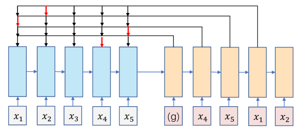
Figure 5: Illustration of the pointer network architecture introduced by Vinyals et al. (2015).

F.4.1 Details of the pointer network

The pointer network is first introduced by (Vinyals et al., 2015) for directly finding solutions of specific combinatorial optimization problems, such as the Travelling Salesman Problems. The pointer network architecture is illustrated in Figure 5. The pointer network consists of a Long Short-Term Memory encoder, a Long Short-Term Memory decoder, and an attention that is used as a pointer to select a member of the input sequence as the output (Vinyals et al., 2015). Specifically, we implement the pointer network following Bello* et al. (2017). Please refer to (Bello* et al., 2017) for implementation details of the pointer network.

The major difference between our used pointer network and the pointer network used in (Bello* et al., 2017) is that we use the pointer network to select ordered subsets of input sequences, but (Bello* et al., 2017) use the pointer network to output permutations of input sequences.

F.4.2 Difference between HEM-ratio and HEM w/o H

Details of HEM w/o H To implement HEM w/o H, we augment each input sequence with an end token, i.e., a thirteen-dimensional tensor with values all being one. The end token is at the end position of the input sequence. Once the decoder of HEM w/o H outputs the end token, then the decoding ends. That is, HEM w/o H can implicitly predict the number of cuts that should be selected by predicting whether to decode the end token at the current decoding step.

The policy network of HEM-ratio and HEM w/o H are both essentially a pointer network (Vinyals et al., 2015), a variant of the sequence model. We present the major difference between HEM-ratio and HEM w/o H in the following. HEM w/o H predicts an end token as used in language tasks (Sutskever et al., 2014; Vaswani et al., 2017) to determine the number of cuts that should be selected implicitly. In contrast, HEM-ratio always selects a fixed ratio of cuts, i.e, it always ends decoding at a pre-determined position. Therefore, HEM w/o H can learn the number of cuts that should be selected, but HEM-ratio cannot.

F.4.3 More discussion of HEM

In this part, we provide details of some more advantages of HEM. (1) Inspired by hierarchical reinforcement learning (Sutton et al., 1999b; Nachum et al., 2018), HEM leverages the hierarchical structure of the cut selection task, which is important for efficient exploration in complex decision-making tasks. (2) Previous methods (Tang et al., 2020; Huang et al., 2022) usually train cut selection policies via black-box optimization methods such as evolution strategies (Salimans et al., 2017). In contrast, HEM is differentiable and we train the HEM via gradient-based algorithms, which is more sample efficient than black-box optimization methods (Sutton & Barto, 2018; Schulman et al., 2015). Although we can offline generate training samples as much as possible using a MILP solver, high sample efficiency is significant as generating samples can be extremely time-consuming in practice.

Appendix G More Results

Table 9: Policy evaluation on easy, medium, and hard datasets in terms of the total number of nodes and the primal-dual gap. The best performance are marked in bold.

	Set Covering		Maximum Independent Set		Multiple Knapsack
Method	Nodes	PD gap	Nodes	PD gap	Nodes	PD gap
NoCuts	189.44 (423.68)	0.00 (0)	2170.66 (4054.09)	0.00 (0)	16945.58 (41242.04)	0.00 (0.000128)
Default	116.77 (420.09)	0.00 (0)	588.23 (1916.99)	0.00 (0)	16949.88 (41297.50)	0.00 (0.000128)
Random	95.70 (285.05)	0.00 (0)	1416.96 (3820.01)	0.00 (0)	21463.16 (59411.07)	0.00 (0.000361)
NV	199.70 (436.25)	0.00 (0)	1618.42 (3089.12)	0.00 (0)	20673.32 (62526.13)	0.00 (0.00022)
Eff	194.17 (439.35)	0.00 (0)	1575.88 (2742.66)	0.00 (0)	14909.93 (28575.12)	0.00 (0)
SBP	1.16 (2.04)	0.00 (0)	698.41 (2869.65)	0.00 (0)	13537.59 (22527.45)	0.00 (0)
HEM (Ours)	1.11 (1.46)	0.00 (0)	311.64 (1309.94)	0.00 (0)	10463.85 (18491.25)	0.00 (0)

	MIK		CORLAT		Load Balancing
Method	Nodes	PD gap	Nodes	PD gap	Nodes	PD gap
NoCuts	395290.17 (120526.21)	0.09 (0.018)	97098.72 (119287.56)	2.000000e+18 (1.4E+19)	108.20 (56.28)	0.94 (0.12)
Default	224746.60 (179450.80)	0.02 (0.033)	70215.01 (113515.62)	2.666667e+18 (1.61E+19)	65.22 (55.34)	0.43 (0.073)
Random	403618.10 (115802.29)	0.07 (0.035)	74149.90 (109043.28)	2.000000e+18 (1.4E+19)	107.05 (68.05)	0.79 (0.133)
NV	397025.47 (106676.73)	0.08 (0.028)	77943.73 (111355.03)	4.666667e+18 (2.11E+19)	81.91 (38.55)	0.82 (0.11)
Eff	406832.83 (113363.27)	0.07 (0.033)	95956.53 (120858.92)	5.333333e+18 (2.25E+19)	86.22 (45.35)	0.82 (0.11)
SBP	417070.37 (133702.50)	0.07 (0.030)	62297.99 (109664.21)	6.666667e+17 (8.14E+18)	138.37 (53.79)	0.65 (0.06)
HEM(Ours)	220547.93 (172537.94)	0.02 (0.028)	51929.71 (100973.74)	0.02 (0.051)	74.47 (60.98)	0.42 (0.072)

	Anonymous		MIPLIB mixed neos		MIPLIB mixed supportcase
Method	Nodes	PD gap	Nodes	PD gap	Nodes	PD gap
NoCuts	20110.58 (14167.51)	8.333333e+18 (2.76E+19)	169348.83 (117745.23)	2.500000e+19 (4.33E+19)	5971.00 (8679.98)	9.19 (19.29)
Default	20025.78 (13056.50)	8.333333e+18 (2.76E+19)	161366.25 (107049.96)	2.500000e+19 (4.33E+19)	4055.04 (7404.61)	11.73 (31.52)
Random	19824.48 (12366.55)	1.000000e+19 (3E+19)	143930.17 (95296.41)	2.500000e+19 (4.33E+19)	4656.13 (7745.46)	6.05 (14.69)
NV	19313.33 (12391.94)	8.333333e+18 (2.76E+19)	150046.50 (94801.62)	2.500000e+19 (4.33E+19)	4986.21 (9024.19)	2.78 (10.08)
Eff	19526.23 (12116.80)	6.666667e+18 (2.49E+19)	144128.83 (93404.76)	2.500000e+19 (4.33E+19)	4450.88 (7845.48)	5.58 (15.40)
SBP	19351.67 (12337.81)	6.666667e+18 (2.49E+19)	177736.25 (122005.81)	2.500000e+19 (4.33E+19)	5618.08 (9765.43)	0.14 (0.26)
HEM(Ours)	20191.28 (13219.21)	1.666667e+18 (1.28E+19)	177735.83 (129020.42)	2.500000e+19 (4.33E+19)	4844.88 (9996.16)	0.14 (0.25)

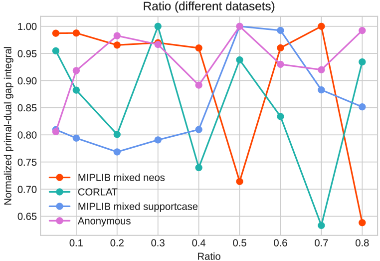
(a) NV with different ratios on four datasets.

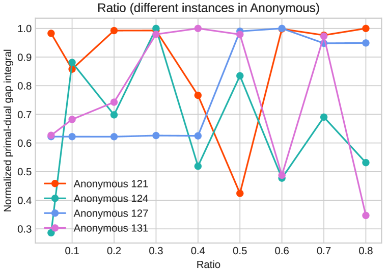
(b) NV with different ratios on Anonymous.

Figure 6: We use the Normalized Violation (NV) rule (Huang et al., 2022). The results in (c) show that NV with different given ratios achieve variable normalized PD integral on four datasets. The results in (d) show that NV with different ratios achieve variable normalized PD integral on different instances from the same dataset.

G.1 More motivating results

Ratio matters. To evaluate the effect of the ratio of selected cuts on solving MILPs, we focus on the Normalized Violation (NV) cut selection method with different ratios of selected cuts. (1) We first evaluate the NV methods that select $5\%,10\%,20\%,30\%,40\%,50\%,60\%,70\%$, and $80\%$ of candidate cuts, respectively, on four datasets. The results in Figure 6(a) show that the NV achieves better solver performance with larger ratios on CORLAT and MIPLIB mixed neos. The results demonstrate that the ratio that leads to better solver performance is variable over different datasets, which implies that learning dataset-dependent ratios is important. (2) We then evaluate the NV methods that select $5\%,10\%,20\%,30\%,40\%,50\%,60\%,70\%$, and $80\%$ of candidate cuts, respectively, on four instances from the Anonymous dataset. The results in Figure 6(b) show that NV achieves better solver performance with larger ratios on Anonymous 121 and Anonymous 131. The results demonstrate that the ratio that leads to better solver performance is variable over different instances from the same dataset, which implies that learning instance-dependent ratios is important as well.

G.2 More results of main evaluation

In this section, we provide more results of the main evaluation. The results in Table 9 show the performance of HEM and the baselines in terms of the total number of nodes (Nodes) and the primal-dual gap (PD gap). (1) Easy datasets. On the easy datasets, HEM and most baselines find the optimal solution within the time limit, as the PD gap converges to zero. Additionally, HEM significantly outperforms all the baselines in terms of the Nodes on the easy datasets. (2) Medium and hard datasets. In terms of the PD gap, HEM outperforms all the baselines on medium and hard datasets, especially on CORLAT. However, the Nodes metric cannot well distinguish the performance of different cut selection methods on the medium and hard datasets for the following two reasons. First, the solving time of the LP relaxation on each node is different, and thus the Nodes cannot directly determine the solving time (Huang et al., 2022). Second, on those unsolved instances within the time limit, the Nodes metric is not a proper metric, as the Nodes cannot evaluate the quality of the solving process.

G.3 More results of ablation study

In this section, we provide more results of ablation studies in the main text.

G.3.1 In-depth analysis of HEM-ratio and SBP

We provide possible reasons for HEM-ratio performing poorer than SBP on several challenging MILP problem benchmarks. Fundamentally, HEM-ratio formulates the cut selection task as a sequence modeling problem, which has two main advantages over SBP. That is, the sequence model can not only capture the underlying order information, but also capture the interaction among cuts. However, training a sequence model is more difficult than training a scoring function, as the sequence model aims to learn a much more complex task. Specifically, the scoring function aims to learn to score each cut, while the sequence model aims to model the joint probability of the selected cuts. The latter is a more challenging learning task. Moreover, we follow the reinforcement learning paradigm instead of supervised learning to train the model, making the training process more unstable. Therefore, the sequence model may suffer from inefficient exploration and be trapped to a local optimum. As a result, HEM-ratio can perform poorer than SBP, especially on challenging MILP problem benchmarks.

G.3.2 Contribution of each component

To understand the contribution of each component of HEM, we provide more results of HEM and HEM without the higher-level model on Set Covering, Multiple Knapsack, MIK, Load Balancing, Anonymous, and MIPLIB mixed supportcase. The results in Table 10 show that HEM outperforms HEM w/o H in terms of the solving time, the primal-dual gap, and the primal-dual gap integral on several challenging datasets, demonstrating the importance of our proposed higher-level model. Moreover, HEM w/o H significantly outperforms SBP in terms of the solving time, the primal-dual gap, and the primal-dual gap integral on several challenging datasets, demonstrating the significance of our proposed lower-level model.

Table 10: Comparsion between HEM, HEM without the higher-level model on more datasets.

	Set Covering				Multiple Knapsack
Method	Time (s)	Nodes	PD gap	PD integral	Time (s)	Nodes	PD gap	PD integral
NoCuts	6.31 (4.61)	189.44 (423.68)	0.00 (0)	56.99 (38.89)	9.88 (22.24)	16945.58 (41242.04)	0.00 (0.000128)	16.41 (14.16)
Default	4.41 (5.12)	116.77 (420.08)	0.00 (0)	55.63 (42.21)	9.90 (22.24)	16949.87 (41297.49)	0.00 (0.000128)	16.46 (14.25)
SBP	1.91 (0.36)	1.16 (2.04)	0.00 (0)	38.96 (8.66)	7.74 (12.36)	13537.58 (22527.45)	0.00 (0)	16.45 (16.62)
HEM w/o H	1.84 (0.31)	1.18 (2.03)	0.00 (0)	37.69 (8.33)	7.36 (12.90)	12418.85 (23256.47)	0.00 (0)	14.01 (10.94)
HEM (Ours)	1.85 (0.31)	1.09 (1.46)	0.00 (0)	37.92 (8.46)	6.13 (9.61)	10463.84 (18491.25)	0.00 (0)	13.63 (9.63)

	MIK				Load Balancing
Method	Time (s)	Nodes	PD gap	PD integral	Time (s)	Nodes	PD gap	PD integral
NoCuts	300.01 (0.009)	395290.16 (120526.21)	0.09 (0.018)	2355.87 (996.08)	300.00 (0.12)	108.20 (56.28)	0.94 (0.12)	14853.77 (951.42)
Default	179.62 (122.36)	224746.60 (179450.80)	0.02 (0.033)	844.40 (924.30)	300.00 (0.06)	65.22 (55.34)	0.43 (0.07)	9589.19 (1012.95)
SBP	286.07 (41.81)	417070.36 (133702.49)	0.07 (0.0295)	2053.30 (740.11)	300.00 (0.10)	138.37 (53.79)	0.65 (0.06)	12535.30 (741.43)
HEM w/o H	218.87 (115.97)	297058.97 (189410.43)	0.04 (0.039)	1321.63 (1165.23)	300.03 (0.04)	70.93 (60.36)	0.42 (0.07)	9475.16 (1005.81)
HEM (Ours)	176.12 (125.18)	220547.93 (172537.94)	0.02 (0.028)	785.04 (790.38)	300.00 (0.04)	74.47 (60.98)	0.42 (0.07)	9496.42 (1018.35)

	Anonymous				MIPLIB mixed supportcase
Method	Time (s)	Nodes	PD gap	PD integral	Time (s)	Nodes	PD gap	PD integral
NoCuts	246.22 (94.90)	20110.58 (14167.51)	8.333333e+18 (2.76E+19)	18297.30 (9769.42)	170.00 (131.60)	5971.00 (8679.98)	9.19 (19.29)	9927.96 (11334.07)
Default	244.02 (97.72)	20025.78 (13056.50)	8.333333e+18 (2.76E+19)	17407.01 (9736.19)	164.61 (135.82)	4055.04 (7404.61)	11.73 (31.52)	9672.34 (10668.24)
SBP	245.71 (92.46)	19351.66 (12337.81)	6.666667e+18 (2.49E+19)	18188.63 (9651.85)	165.61 (135.25)	5618.08 (9765.43)	0.14 (0.26)	7408.65 (7903.47)
HEM w/o H	251.00 (88.45)	21192.40 (16436.32)	5.000000e+18 (2.18E+19)	17226.84 (9553.90)	156.96 (133.35)	3779.83 (7465.75)	0.56 (1.43)	7709.19 (8655.48)
HEM (Ours)	241.68 (97.23)	20191.28 (13219.21)	1.666667e+18 (1.28E+19)	16077.15 (9108.21)	162.96 (138.21)	4844.87 (9996.15)	0.14 (0.25)	6874.80 (6729.97)

Table 11: Comparsion between HEM, HEM-ratio, and HEM-ratio-order on more datasets.

	Set Covering				Multiple Knapsack
Method	Time (s)	Nodes	PD gap	PD integral	Time (s)	Nodes	PD gap	PD integral
NoCuts	6.31 (4.61)	189.44 (423.68)	0.00 (0)	56.99 (38.89)	9.88 (22.24)	16945.58 (41242.04)	0.00 (0.000128)	16.41 (14.16)
Default	4.41 (5.12)	116.77 (420.08)	0.00 (0)	55.63 (42.21)	9.90 (22.24)	16949.87 (41297.49)	0.00 (0.000128)	16.46 (14.25)
SBP	1.91 (0.36)	1.16 (2.04)	0.00 (0)	38.96 (8.66)	7.74 (12.36)	13537.58 (22527.45)	0.00 (0)	16.45 (16.62)
HEM-ratio-order	2.11 (0.38)	1.11 (1.29)	0.00 (0)	42.01 (9.88)	10.46 (29.74)	18434.20 (59254.10)	0.00 (0.000128)	16.92 (18.19)
HEM-ratio	2.10 (0.40)	1.11 (1.18)	0.00 (0)	41.95 (9.82)	7.63 (12.64)	13307.73 (24339.3)	0.00 (0)	16.19 (15.16)
HEM (Ours)	1.85 (0.31)	1.09 (1.46)	0.00 (0)	37.92 (8.46)	6.13 (9.61)	10463.84 (18491.25)	0.00 (0)	13.63 (9.63)

	MIK				Load Balancing
Method	Time (s)	Nodes	PD gap	PD integral	Time (s)	Nodes	PD gap	PD integral
NoCuts	300.01 (0.009)	395290.16 (120526.21)	0.09 (0.018)	2355.87 (996.08)	300.00 (0.12)	108.20 (56.28)	0.94 (0.12)	14853.77 (951.42)
Default	179.62 (122.36)	224746.60 (179450.80)	0.02 (0.033)	844.40 (924.30)	300.00 (0.06)	65.22 (55.34)	0.43 (0.07)	9589.19 (1012.95)
SBP	286.07 (41.81)	417070.36 (133702.49)	0.07 (0.0295)	2053.30 (740.11)	300.00 (0.10)	138.37 (53.79)	0.65 (0.06)	12535.30 (741.43)
HEM-ratio-order	282.92 (42.07)	417397.10 (132077.3)	0.06 (0.034)	2072.69 (849.16)	300.11 (0.11)	145.18 (56.52)	0.65 (0.061)	12368.12 (726.77)
HEM-ratio	283.75 (39.87)	401540.97 (131295.8)	0.07 (0.034)	1869.66 (978.85)	300.10 (0.098)	148.92 (59.12)	0.65 (0.058)	12410.84 (715.44)
HEM (Ours)	176.12 (125.18)	220547.93 (172537.94)	0.02 (0.028)	785.04 (790.38)	300.00 (0.04)	74.47 (60.98)	0.42 (0.07)	9496.42 (1018.35)

	Anonymous				MIPLIB mixed supportcase
Method	Time (s)	Nodes	PD gap	PD integral	Time (s)	Nodes	PD gap	PD integral
NoCuts	246.22 (94.90)	20110.58 (14167.51)	8.33e+18 (2.76E+19)	18297.30 (9769.42)	170.00 (131.60)	5971.00 (8679.98)	9.19 (19.29)	9927.96 (11334.07)
Default	244.02 (97.72)	20025.78 (13056.50)	8.33e+18 (2.76E+19)	17407.01 (9736.19)	164.61 (135.82)	4055.04 (7404.61)	11.73 (31.52)	9672.34 (10668.24)
SBP	245.71 (92.46)	19351.66 (12337.81)	6.67e+18 (2.49E+19)	18188.63 (9651.85)	165.61 (135.25)	5618.08 (9765.43)	0.14 (0.26)	7408.65 (7903.47)
HEM-ratio-order	245.45 (94.99)	20495.80 (12472.44)	5.00e+18 (2.18E+19)	16496.06 (9282.15)	169.45 (132.55)	6252.63 (9827.98)	4.25 (15.97)	9226.95 (9995.94)
HEM-ratio	245.17 (95.21)	20942.07 (13379.46)	5.00e+18 (2.18E+19)	16148.82 (9247.48)	163.03 (137.16)	5551.29 (10708.46)	7.54 (21.85)	9979.35 (11048.11)
HEM (Ours)	241.68 (97.23)	20191.28 (13219.21)	1.67e+18 (1.28E+19)	16077.15 (9108.21)	162.96 (138.21)	4844.87 (9996.15)	0.14 (0.25)	6874.80 (6729.97)

Table 12: Sensitivity analysis of HEM to the hyperparameter dealy update freq $d$.

	Maximum Independent Set			Corlat			MIPLIBS Mixed (neos)
Method	Time(s)	PD integral	Improvement (PD integral, %)	Time(s)	PD integral	Improvement (PD integral, %)	Time(s)	PD integral	Improvement (PD integral, %)
NoCuts	8.78 (6.66)	71.31 (51.74)	NA	103.30 (128.14)	2818.40 (5908.31)	NA	253.65 (80.29)	14652.29 (12523.37)	NA
HEM (delay=1)	1.79 (3.65)	16.56 (26.6)	76.78	57.39 (111.76)	1260.83 (3518.07)	55.26	254.48 (78.84)	9273.01 (12031.44)	36.71
HEM (delay=2)	1.76 (3.69)	16.01 (26.21)	77.55	58.31 (110.51)	1079.99 (2653.14)	61.68	248.66 (89.46)	8678.76 (12337.00)	40.77
HEM (delay=3)	1.80 (3.82)	16.91 (28.49)	76.29	58.50 (108.88)	1003.52 (2264.91)	64.39	247.62 (90.73)	8408.16 (12467.02)	42.62
HEM (delay=4)	1.89 (3.90)	17.34 (28.46)	75.68	69.60 (115.42)	1309.33 (3336.59)	53.54	246.93 (91.93)	8368.46 (12489.68)	42.89

Table 13: Evaluate the generalization ability of HEM on Set Covering.

	Set Covering ($2\times$)			Set Covering ($4\times$)
Method	Time(s) $\downarrow$	Improvement $\uparrow$ (time, %)	PD integral $\downarrow$	Time(s) $\downarrow$	Improvement $\uparrow$ (time, %)	PD integral $\downarrow$
NoCuts	82.69 (78.27)	NA	609.43 (524.92)	284.44 (48.70)	NA	3215.34 (1019.47)
Default	61.01 (78.12)	26.22	494.63 (545.76)	149.69 ( 141.92)	47.37	1776.22 (1651.15)
Random	64.44 (73.98)	22.07	520.84 (489.52)	208.12 (131.52)	26.53	2528.36 (1678.66)
NV	92.05 (80.11)	-11.32	725.53 (541.68)	286.10 (45.47)	-0.58	3422.46 (1024.19)
Eff	92.32 (79.33)	-11.64	733.72 (538.60)	286.20 (45.04)	-0.62	3437.06 (1043.44)
SBP	3.52 (1.36)	95.74	92.89 (25.83)	7.62 (6.46)	97.32	256.79 (145.92)
HEM (Ours)	3.33 (0.47)	95.97	89.24 (14.26)	7.40 (5.03)	97.40	250.83 (131.43)

G.3.3 The importance of tackling P1-P3 in cut selection

To understand the importance of tackling P1-P3 in cut selection, we provide more results of HEM, HEM-ratio, and HEM-ratio-order on Set Covering, Multiple Knapsack, MIK, Load Balancing, Anonymous, and MIPLIB mixed supportcase. Here we refresh what HEM, HEM-ratio, HEM-ratio-order mean. (1) HEM. HEM tackles P1-P3 in cut selection simultaneously. (2) HEM-ratio. In order not to learn how many cuts should be selected, we remove the higher-level model of HEM and force the lower-level model to select a fixed ratio of cuts. We denote it by HEM-ratio. Note that HEM-ratio is different from HEM w/o H (see Appendix F). HEM-ratio tackles P1 and P3 in cut selection. (3) HEM-ratio-order. To further mute the effect of the order of selected cuts, we reorder the selected cuts given by HEM-ratio with the original index of the generated cuts, which we denote by HEM-ratio-order. HEM-ratio-order mainly tackles P1.

The results in Table 11 suggest the following. HEM-ratio-order outperforms Default and NoCuts on several datasets, demonstrating that tackling P1 by data-driven methods is crucial. HEM significantly outperforms HEM-ratio in terms of the primal-dual gap integral, demonstrating the significance of tackling P2. HEM-ratio outperforms HEM-ratio-order on several datasets, which demonstrates the importance of tackling P3. Moreover, HEM-ratio performs better than SBP in terms of the solving time and the primal-dual gap integral on all six datasets except Set Covering and MIPLIB mixed supportcase, which shows the superiority of formulating the cut selection as a sequence to sequence learning problem over formulating it as a scoring task. However, HEM-ratio and HEM-ratio-order perform a little worse than SBP on Set Covering and MIPLIB mixed supportcase. A possible reason is that it is more difficult to train a sequence model than to train a multi-layer perceptron and thus the sequence model may suffer from inefficient exploration and be trapped to the local optimum. Please refer to Appendix G.3.1 for a detailed analysis.

G.3.4 Sensitivity analysis

Additionally, we perform ablation studies to test the sensitivity of HEM to the hyperparameter delay update freq $d$. The results in Table 12 show that there is a wide range of $d$ for HEM to achieve comparable performance on Maximum Independent Set, CORLAT, and MIPLIB mixed neos. Moreover, we emphasize that we do not tune the hyperparameter $d$. As the results shown in Table 12, $d=3$ and $d=4$ performs the best on CORLAT and MIPLIB mixed neos, respectively. However, we simply set $d=2$ throughout all experiments in the main text.

G.4 More results of generalization

Here we provide more results of the generalization experiments on Set Covering. On Set Covering, we test HEM on two times and four times larger instances than those seen during training. The results in Table 13 show that HEM generalizes well to instances that are significantly larger than seen during training. In particular, HEM achieves at least $70\%$ improvement in terms of the Time compared to all the rule-based baselines. Moreover, SBP also generalizes well to large instances, demonstrating that SBP is a strong baseline.

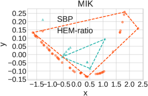
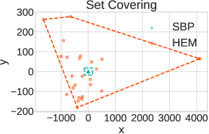
Figure 7: We perform principal component analysis on cuts selected by HEM-ratio/HEM and SBP. Each colored point illustrates a reduced cut feature. To visualize the diversity of selected cuts, we use dashed lines to connect the points with the smallest and largest x,y coordinates.

G.5 More visualization results

In this part, we provide more visualization results on Set Covering and MIK. On MIK, we visualize the cuts selected by HEM-ratio and SBP on a randomly sampled instance. We perform principal component analysis (Mohri et al., 2018) on selected cuts to reduce the cut features to two-dimensional space. Colored points illustrate reduced cut features. To visualize the diversity of selected cuts, we use dashed lines to connect the points with the smallest and largest x,y coordinates. The results in Figure 7 still show that HEM-ratio selects much more diverse cuts than SBP on MIK. However, HEM-ratio performs poorer than SBP on Set Covering (see Appendix G.3.1 for a detailed analysis). Therefore, we visualize the cuts selected by HEM and SBP on a randomly sampled instance from Set Covering. Although HEM learns the number of cuts that should be selected, we find that HEM selects much fewer cuts than SBP. Specifically, HEM selects 25 cuts, while SBP selects 158 cuts. Interestingly, the results in Figure 7 show that SBP selects 158 similar cuts with high scores, while HEM selects much more diverse cuts than SBP. The results show that HEM tends to select cuts that complement each other nicely.

Table 14: Policy evaluation on MIPLIB mixed neos and MIPLIB mixed supportcase with a time limit of three hours.

	MIPLIB mixed neos					MIPLIB mixed supportcase
Method	Time (s)	Nodes	PD gap	PD integral	Improvement (PD integral, %)	Time (s)	Nodes	PD gap	PD integral	Improvement (PD integral, %)
NoCuts	8,126.15 (4631.32)	5,058,282.42 (5067358)	0.97 (1.14)	369,180.71 (368274)	NA	3,616.09 (4703.68)	258,543.71 (692821)	0.00 (0.0096)	37,858.65 (59578.6)	NA
Default	8,129.27 (4625.92)	4,800,372.67 (4815222)	0.94 (1.07)	392,324.09 (393266)	-6.27	3,997.69 (4720.2)	188,844.71 (599665)	0.01 (0.012)	56,375.64 (106694)	-48.91
Random	8,125.44 (4632.53)	5,107,627.25 (5114152)	0.95 (1.09)	395,694.74 (393445)	-7.18	2,605.78 (3993.84)	8,458.96 (14785.9)	0.01 (0.029)	44,222.39 (70937.6)	-16.81
NV	8,133.64 (4618.37)	4,930,498.92 (4930971)	0.91 (1.03)	326,315.04 (391163)	11.61	2,561.10 (3980.44)	34,851.08 (142069)	0.00 (0.0095)	27,908.00 (37742.2)	26.28
Eff	8,130.78 (4623.31)	4,788,568.75 (4804443)	0.94 (1.07)	395,640.44 (393572)	-7.17	3,105.98 (4308.57)	182,187.63 (543167)	0.01 (0.028)	39,932.37 (58307.3)	-5.48
SBP	8,130.63 (4626.62)	4,763,378.00 (4829037)	0.91 (1.03)	388,564.35 (398176.3)	-5.25	3,014.63 (4082.19)	146,180.96 (543662.45)	0.00 (0.0084)	24,447.37 (55984.9)	35.42
HEM(Ours)	8,124.32 (4634.54)	4,748,599.50 (4816327)	0.78 (0.82)	194,557.87 (345035)	47.30	3,465.48 (4485.11)	52,750.08 (140410)	0.00 (0.0087)	17,885.98 (24045.9)	52.76

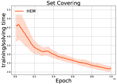
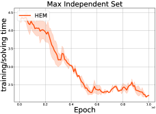
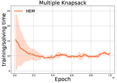
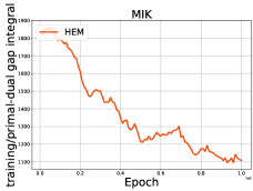
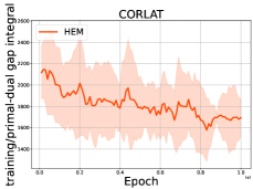
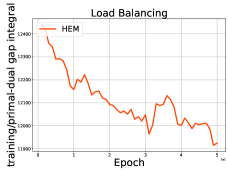
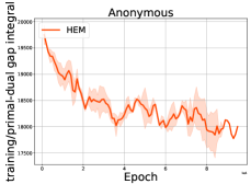
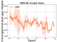
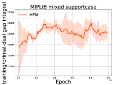
Figure 8: Training curves of HEM on all nine datasets. The x-axis corresponds to the training epochs. The y-axis corresponds to the average solving time on easy datasets and the primal-dual gap integral on the other datasets. The solid curves correspond to the mean and the shaded region to the standard deviation over three random seeds. For visual clarity, we smooth curves.

G.6 Evaluation with a time limit of three hours

In this section, we aim to evaluate whether HEM can generalize well to solving problems within a much longer time limit. Specifically, we evaluate HEM on two extremely challenging MIPLIB datasets within a time limit of three hours. Note that we still train HEM with a time limit of 300 seconds, while we test HEM with a time limit of three hours. The results in Table 14 show that HEM still significantly outperforms all the baselines, especially in terms of the primal-dual gap integral on MIPLIB mixed neos and MIPLIB mixed supportcase. In terms of the primal-dual gap, HEM also outperforms the baselines. Moreover, HEM performs better than baselines in terms of the solving time on MIPLIB mixed neos, but HEM performs poorly in terms of the solving time on MIPLIB mixed supportcase. Interestingly, the primal-dual gap integral is not always consistent with the solving time. We emphasize that we train with the negative primal-dual gap integral reward. To further improve the performance of HEM in terms of the solving time, we can set the reward as the negative solving time instead of the negative primal-dual gap integral.

G.7 Training curves

In this section, we provide the training curves of HEM on all nine datasets. The results in Figure 8 show that the performance of our learned policies in terms of the solving time or the primal-dual gap integral drops with the training epochs, demonstrating the effectiveness of our learning process.

References

- Achterberg (2007) Tobias Achterberg. Constraint integer programming. 2007.
- Atamtürk (2003) Alper Atamtürk. On the facets of the mixed–integer knapsack polyhedron. Mathematical Programming, 98(1):145–175, 2003.
- Balas & Ho (1980) Egon Balas and Andrew Ho. Set covering algorithms using cutting planes, heuristics, and subgradient optimization: a computational study. In Combinatorial Optimization, pp. 37–60. Springer, 1980.
- Balcan et al. (2018) Maria-Florina Balcan, Travis Dick, Tuomas Sandholm, and Ellen Vitercik. Learning to branch. In Jennifer Dy and Andreas Krause (eds.), Proceedings of the 35th International Conference on Machine Learning, volume 80 of Proceedings of Machine Learning Research, pp. 344–353. PMLR, 10–15 Jul 2018.
- Balcan et al. (2021) Maria-Florina F Balcan, Siddharth Prasad, Tuomas Sandholm, and Ellen Vitercik. Sample complexity of tree search configuration: Cutting planes and beyond. Advances in Neural Information Processing Systems, 34:4015–4027, 2021.
- Baltean-Lugojan et al. (2019) Radu Baltean-Lugojan, Pierre Bonami, Ruth Misener, and Andrea Tramontani. Scoring positive semidefinite cutting planes for quadratic optimization via trained neural networks. preprint: http://www. optimization-online. org/DB_ HTML/2018/11/6943. html, 2019.
- Bello* et al. (2017) Irwan Bello*, Hieu Pham*, Quoc V. Le, Mohammad Norouzi, and Samy Bengio. Neural combinatorial optimization with reinforcement learning, 2017.
- Bengio et al. (2021) Yoshua Bengio, Andrea Lodi, and Antoine Prouvost. Machine learning for combinatorial optimization: a methodological tour d’horizon. European Journal of Operational Research, 290(2):405–421, 2021.
- Bergman et al. (2016) David Bergman, Andre A Cire, Willem-Jan Van Hoeve, and John Hooker. Decision diagrams for optimization, volume 1. Springer, 2016.
- Bestuzheva et al. (2021) Ksenia Bestuzheva, Mathieu Besançon, Wei-Kun Chen, Antonia Chmiela, Tim Donkiewicz, Jasper van Doornmalen, Leon Eifler, Oliver Gaul, Gerald Gamrath, Ambros Gleixner, et al. The scip optimization suite 8.0. arXiv preprint arXiv:2112.08872, 2021.
- Bixby (1992) Robert E Bixby. Implementing the simplex method: The initial basis. ORSA Journal on Computing, 4(3):267–284, 1992.
- Bixby et al. (2004) Robert E Bixby, Mary Fenelon, Zonghao Gu, Ed Rothberg, and Roland Wunderling. Mixed-integer programming: A progress report. In The sharpest cut: the impact of Manfred Padberg and his work, pp. 309–325. SIAM, 2004.
- Bowly et al. (2021) Simon Bowly, Quentin Cappart, Jonas Charfreitag, Laurent Charlin, Didier Chételat, Antonia Chmiela, Justin Dumouchelle, Maxime Gasse, Ambros Gleixner, Aleksandr M, Kazachkov, Elias B, Khalil, Pawel Lichocki, Andrea Lodi, Miles Lubin, Chris J, Maddison, Christopher Morris, Dimitri J, Papageorgiou, Augustin Parjadis, Sebastian Pokutta, Antoine Prouvost, Lara Scavuzzo, and Giulia Zarpellon. Machine learning for combinatorial optimization, 2021. URL https://www.ecole.ai/2021/ml4co-competition/.
- Cao et al. (2022) Zixuan Cao, Yang Xu, Zhewei Huang, and Shuchang Zhou. Ml4co-kida: Knowledge inheritance in dataset aggregation. arXiv preprint arXiv:2201.10328, 2022.
- Chen (2021) Lei Chen. Deep Learning and Practice with MindSpore. Springer Nature, 2021.
- Chen (2010) Zhi-Long Chen. Integrated production and outbound distribution scheduling: review and extensions. Operations research, 58(1):130–148, 2010.
- Dey & Molinaro (2018a) Santanu S Dey and Marco Molinaro. Theoretical challenges towards cutting-plane selection. Mathematical Programming, 170(1):237–266, 2018a.
- Dey & Molinaro (2018b) Santanu S Dey and Marco Molinaro. Theoretical challenges towards cutting-plane selection. Mathematical Programming, 170(1):237–266, 2018b.
- Farahani & Hekmatfar (2009) Reza Zanjirani Farahani and Masoud Hekmatfar. Facility location: concepts, models, algorithms and case studies. Springer Science & Business Media, 2009.
- FICO Xpress (2020) FICO Xpress. Xpress optimization suite, https://www.fico.com/en/products/fico-xpress-optimization, 2020.
- Fujimoto et al. (2018) Scott Fujimoto, Herke van Hoof, and David Meger. Addressing function approximation error in actor-critic methods. In Jennifer Dy and Andreas Krause (eds.), Proceedings of the 35th International Conference on Machine Learning, volume 80 of Proceedings of Machine Learning Research, pp. 1587–1596. PMLR, 10–15 Jul 2018.
- Gasse et al. (2019) Maxime Gasse, Didier Chetelat, Nicola Ferroni, Laurent Charlin, and Andrea Lodi. Exact combinatorial optimization with graph convolutional neural networks. In H. Wallach, H. Larochelle, A. Beygelzimer, F. d'Alché-Buc, E. Fox, and R. Garnett (eds.), Advances in Neural Information Processing Systems, volume 32. Curran Associates, Inc., 2019.
- Gleixner et al. (2021) Ambros Gleixner, Gregor Hendel, Gerald Gamrath, Tobias Achterberg, Michael Bastubbe, Timo Berthold, Philipp Christophel, Kati Jarck, Thorsten Koch, Jeff Linderoth, et al. Miplib 2017: data-driven compilation of the 6th mixed-integer programming library. Mathematical Programming Computation, 13(3):443–490, 2021.
- Gomes et al. (2008) Carla P Gomes, Willem-Jan van Hoeve, and Ashish Sabharwal. Connections in networks: A hybrid approach. In International Conference on Integration of Artificial Intelligence (AI) and Operations Research (OR) Techniques in Constraint Programming, pp. 303–307. Springer, 2008.
- Gomory (1960) Ralph Gomory. An algorithm for the mixed integer problem. Technical report, RAND CORP SANTA MONICA CA, 1960.
- Goodfellow et al. (2016) Ian Goodfellow, Yoshua Bengio, and Aaron Courville. Deep learning. MIT press, 2016.
- Gupta et al. (2022) Prateek Gupta, Elias B Khalil, Didier Chetélat, Maxime Gasse, Yoshua Bengio, Andrea Lodi, and M Pawan Kumar. Lookback for learning to branch. arXiv preprint arXiv:2206.14987, 2022.
- Gurobi (2021) Gurobi. Gurobi solver, https://www.gurobi.com/, 2021.
- Haarnoja et al. (2018) Tuomas Haarnoja, Aurick Zhou, Pieter Abbeel, and Sergey Levine. Soft actor-critic: Off-policy maximum entropy deep reinforcement learning with a stochastic actor. In Jennifer Dy and Andreas Krause (eds.), Proceedings of the 35th International Conference on Machine Learning, volume 80 of Proceedings of Machine Learning Research, pp. 1861–1870. PMLR, 10–15 Jul 2018.
- He et al. (2014) He He, Hal Daume III, and Jason M Eisner. Learning to search in branch and bound algorithms. In Z. Ghahramani, M. Welling, C. Cortes, N. Lawrence, and K.Q. Weinberger (eds.), Advances in Neural Information Processing Systems, volume 27. Curran Associates, Inc., 2014.
- Hendel et al. (2019) Gregor Hendel, Matthias Miltenberger, and Jakob Witzig. Adaptive algorithmic behavior for solving mixed integer programs using bandit algorithms. In Operations Research Proceedings 2018, pp. 513–519. Springer, 2019.
- Hochreiter & Schmidhuber (1997) Sepp Hochreiter and Jürgen Schmidhuber. Long short-term memory. Neural computation, 9(8):1735–1780, 1997.
- Huang et al. (2022) Zeren Huang, Kerong Wang, Furui Liu, Hui-Ling Zhen, Weinan Zhang, Mingxuan Yuan, Jianye Hao, Yong Yu, and Jun Wang. Learning to select cuts for efficient mixed-integer programming. Pattern Recognition, 123:108353, 2022. ISSN 0031-3203. doi: https://doi.org/10.1016/j.patcog.2021.108353.
- Hutter et al. (2010) Frank Hutter, Holger H Hoos, and Kevin Leyton-Brown. Automated configuration of mixed integer programming solvers. In International Conference on Integration of Artificial Intelligence (AI) and Operations Research (OR) Techniques in Constraint Programming, pp. 186–202. Springer, 2010.
- Jünger et al. (2009) Michael Jünger, Thomas M Liebling, Denis Naddef, George L Nemhauser, William R Pulleyblank, Gerhard Reinelt, Giovanni Rinaldi, and Laurence A Wolsey. 50 Years of integer programming 1958-2008: From the early years to the state-of-the-art. Springer Science & Business Media, 2009.
- Khalil et al. (2016) Elias Khalil, Pierre Le Bodic, Le Song, George Nemhauser, and Bistra Dilkina. Learning to branch in mixed integer programming. Proceedings of the AAAI Conference on Artificial Intelligence, 30(1), Feb. 2016. doi: 10.1609/aaai.v30i1.10080. URL https://ojs.aaai.org/index.php/AAAI/article/view/10080.
- Khalil et al. (2017) Elias B Khalil, Bistra Dilkina, George L Nemhauser, Shabbir Ahmed, and Yufen Shao. Learning to run heuristics in tree search. In Ijcai, pp. 659–666, 2017.
- Kingma & Ba (2014) Diederik P Kingma and Jimmy Ba. Adam: A method for stochastic optimization. arXiv preprint arXiv:1412.6980, 2014.
- Konda & Tsitsiklis (2003) VR Konda and JN Tsitsiklis. On actor-critic algorithms. SIAM Journal on Control and Optimization, 42(4):1143–1166, 2003.
- Land & Doig (2010) Ailsa H Land and Alison G Doig. An automatic method for solving discrete programming problems. In 50 Years of Integer Programming 1958-2008, pp. 105–132. Springer, 2010.
- Laporte (2009) Gilbert Laporte. Fifty years of vehicle routing. Transportation science, 43(4):408–416, 2009.
- Lenstra & Shmoys (2009) Jan Karel Lenstra and David Shmoys. The traveling salesman problem: A computational study, 2009.
- Li et al. (2022) Xijun Li, Qingyu Qu, Fangzhou Zhu, Jia Zeng, Mingxuan Yuan, Kun Mao, and Jie Wang. Learning to reformulate for linear programming. arXiv preprint arXiv:2201.06216, 2022.
- Lodi & Zarpellon (2017) Andrea Lodi and Giulia Zarpellon. On learning and branching: a survey. Top, 25(2):207–236, 2017.
- Maros (2002) István Maros. Computational techniques of the simplex method, volume 61. Springer Science & Business Media, 2002.
- Mitchell (2002) John E Mitchell. Branch-and-cut algorithms for combinatorial optimization problems. Handbook of applied optimization, 1(1):65–77, 2002.
- Mnih et al. (2016) Volodymyr Mnih, Adria Puigdomenech Badia, Mehdi Mirza, Alex Graves, Timothy Lillicrap, Tim Harley, David Silver, and Koray Kavukcuoglu. Asynchronous methods for deep reinforcement learning. In Maria Florina Balcan and Kilian Q. Weinberger (eds.), Proceedings of The 33rd International Conference on Machine Learning, volume 48 of Proceedings of Machine Learning Research, pp. 1928–1937, New York, New York, USA, 20–22 Jun 2016. PMLR.
- Mohri et al. (2018) Mehryar Mohri, Afshin Rostamizadeh, and Ameet Talwalkar. Foundations of machine learning. MIT press, 2018.
- Morabit et al. (2021) Mouad Morabit, Guy Desaulniers, and Andrea Lodi. Machine-learning-based column selection for column generation. Transportation Science, 55(4):815–831, 2021.
- Nachum et al. (2018) Ofir Nachum, Shixiang Shane Gu, Honglak Lee, and Sergey Levine. Data-efficient hierarchical reinforcement learning. Advances in neural information processing systems, 31, 2018.
- Nair et al. (2020) Vinod Nair, Sergey Bartunov, Felix Gimeno, Ingrid von Glehn, Pawel Lichocki, Ivan Lobov, Brendan O’Donoghue, Nicolas Sonnerat, Christian Tjandraatmadja, Pengming Wang, et al. Solving mixed integer programs using neural networks. arXiv preprint arXiv:2012.13349, 2020.
- Paschos (2014) Vangelis Th Paschos. Applications of combinatorial optimization, volume 3. John Wiley & Sons, 2014.
- Paszke et al. (2019) Adam Paszke, Sam Gross, Francisco Massa, Adam Lerer, James Bradbury, Gregory Chanan, Trevor Killeen, Zeming Lin, Natalia Gimelshein, Luca Antiga, Alban Desmaison, Andreas Kopf, Edward Yang, Zachary DeVito, Martin Raison, Alykhan Tejani, Sasank Chilamkurthy, Benoit Steiner, Lu Fang, Junjie Bai, and Soumith Chintala. Pytorch: An imperative style, high-performance deep learning library. In H. Wallach, H. Larochelle, A. Beygelzimer, F. d'Alché-Buc, E. Fox, and R. Garnett (eds.), Advances in Neural Information Processing Systems, volume 32. Curran Associates, Inc., 2019.
- Paulus et al. (2022) Max B Paulus, Giulia Zarpellon, Andreas Krause, Laurent Charlin, and Chris Maddison. Learning to cut by looking ahead: Cutting plane selection via imitation learning. In Kamalika Chaudhuri, Stefanie Jegelka, Le Song, Csaba Szepesvari, Gang Niu, and Sivan Sabato (eds.), Proceedings of the 39th International Conference on Machine Learning, volume 162 of Proceedings of Machine Learning Research, pp. 17584–17600. PMLR, 17–23 Jul 2022.
- Pochet & Wolsey (2006) Yves Pochet and Laurence A Wolsey. Production planning by mixed integer programming, volume 149. Springer, 2006.
- Sabharwal et al. (2012) Ashish Sabharwal, Horst Samulowitz, and Chandra Reddy. Guiding combinatorial optimization with uct. In International conference on integration of artificial intelligence (AI) and operations research (OR) techniques in constraint programming, pp. 356–361. Springer, 2012.
- Salimans et al. (2017) Tim Salimans, Jonathan Ho, Xi Chen, Szymon Sidor, and Ilya Sutskever. Evolution strategies as a scalable alternative to reinforcement learning. arXiv preprint arXiv:1703.03864, 2017.
- Scavuzzo et al. (2022) Lara Scavuzzo, Feng Yang Chen, Didier Chételat, Maxime Gasse, Andrea Lodi, Neil Yorke-Smith, and Karen Aardal. Learning to branch with tree mdps. arXiv preprint arXiv:2205.11107, 2022.
- Schulman et al. (2015) John Schulman, Sergey Levine, Pieter Abbeel, Michael Jordan, and Philipp Moritz. Trust region policy optimization. In Francis Bach and David Blei (eds.), Proceedings of the 32nd International Conference on Machine Learning, volume 37 of Proceedings of Machine Learning Research, pp. 1889–1897, Lille, France, 07–09 Jul 2015. PMLR.
- Schulman et al. (2017) John Schulman, Filip Wolski, Prafulla Dhariwal, Alec Radford, and Oleg Klimov. Proximal policy optimization algorithms. arXiv preprint arXiv:1707.06347, 2017.
- Sun et al. (2020) Haoran Sun, Wenbo Chen, Hui Li, and Le Song. Improving learning to branch via reinforcement learning. In Learning Meets Combinatorial Algorithms at NeurIPS2020, 2020.
- Sutskever et al. (2014) Ilya Sutskever, Oriol Vinyals, and Quoc V Le. Sequence to sequence learning with neural networks. In Z. Ghahramani, M. Welling, C. Cortes, N. Lawrence, and K.Q. Weinberger (eds.), Advances in Neural Information Processing Systems, volume 27. Curran Associates, Inc., 2014.
- Sutton & Barto (2018) Richard S Sutton and Andrew G Barto. Reinforcement learning: An introduction. MIT press, 2018.
- Sutton et al. (1999a) Richard S Sutton, David McAllester, Satinder Singh, and Yishay Mansour. Policy gradient methods for reinforcement learning with function approximation. Advances in neural information processing systems, 12, 1999a.
- Sutton et al. (1999b) Richard S Sutton, Doina Precup, and Satinder Singh. Between mdps and semi-mdps: A framework for temporal abstraction in reinforcement learning. Artificial intelligence, 112(1-2):181–211, 1999b.
- Tang et al. (2020) Yunhao Tang, Shipra Agrawal, and Yuri Faenza. Reinforcement learning for integer programming: Learning to cut. In Hal Daumé III and Aarti Singh (eds.), Proceedings of the 37th International Conference on Machine Learning, volume 119 of Proceedings of Machine Learning Research, pp. 9367–9376. PMLR, 13–18 Jul 2020.
- Turner et al. (2022) Mark Turner, Thorsten Koch, Felipe Serrano, and Michael Winkler. Adaptive cut selection in mixed-integer linear programming. arXiv preprint arXiv:2202.10962, 2022.
- Vaswani et al. (2017) Ashish Vaswani, Noam Shazeer, Niki Parmar, Jakob Uszkoreit, Llion Jones, Aidan N Gomez, Ł ukasz Kaiser, and Illia Polosukhin. Attention is all you need. In I. Guyon, U. Von Luxburg, S. Bengio, H. Wallach, R. Fergus, S. Vishwanathan, and R. Garnett (eds.), Advances in Neural Information Processing Systems, volume 30. Curran Associates, Inc., 2017.
- Vinyals et al. (2015) Oriol Vinyals, Meire Fortunato, and Navdeep Jaitly. Pointer networks. In C. Cortes, N. Lawrence, D. Lee, M. Sugiyama, and R. Garnett (eds.), Advances in Neural Information Processing Systems, volume 28. Curran Associates, Inc., 2015.
- Vinyals et al. (2016) Oriol Vinyals, Samy Bengio, and Manjunath Kudlur. Order matters: Sequence to sequence for sets. In Yoshua Bengio and Yann LeCun (eds.), 4th International Conference on Learning Representations, ICLR 2016, San Juan, Puerto Rico, May 2-4, 2016, Conference Track Proceedings, 2016. URL http://arxiv.org/abs/1511.06391.
- Wesselmann & Stuhl (2012) Franz Wesselmann and U Stuhl. Implementing cutting plane management and selection techniques. In Technical Report. University of Paderborn, 2012.
- Zarpellon et al. (2021) Giulia Zarpellon, Jason Jo, Andrea Lodi, and Yoshua Bengio. Parameterizing branch-and-bound search trees to learn branching policies. In Proceedings of the AAAI Conference on Artificial Intelligence, volume 35, pp. 3931–3939, 2021.