Approximating Red-Blue Set Cover and Minimum Monotone Satisfying Assignment

Abstract

We provide new approximation algorithms for the Red-Blue Set Cover and Circuit Minimum Monotone Satisfying Assignment (MMSA) problems. Our algorithm for Red-Blue Set Cover achieves $\tilde{O}(m^{1/3})$-approximation improving on the $\tilde{O}(m^{1/2})$-approximation due to Elkin and Peleg (where $m$ is the number of sets). Our approximation algorithm for MMSA_t (for circuits of depth $t$) gives an $\tilde{O}(N^{1-\delta})$ approximation for $\delta=\frac{1}{3}2^{3-\lceil t/2\rceil}$, where $N$ is the number of gates and variables. No non-trivial approximation algorithms for MMSA_t with $t\geq 4$ were previously known.

We complement these results with lower bounds for these problems: For Red-Blue Set Cover, we provide a nearly approximation preserving reduction from Min $k$-Union that gives an $\tilde{\Omega}(m^{1/4-\varepsilon})$ hardness under the Dense-vs-Random conjecture, while for MMSA we sketch a proof that an SDP relaxation strengthened by Sherali–Adams has an integrality gap of $N^{1-\varepsilon}$ where $\varepsilon\to 0$ as the circuit depth $t\to\infty$.

1 Introduction

In this paper, we study two problems, Red-Blue Set Cover and its generalization Circuit Minimum Monotone Satisfying Assignment. Red-Blue Set Cover, a natural generalization of Set Cover, was introduced by Carr et al. (2000). Circuit Minimum Monotone Satisfying Assignment, a problem more closely related to Label Cover, was introduced by Alekhnovich et al. (2001) and Goldwasser and Motwani (1997).

Definition 1.1.

In Red-Blue Set Cover, we are given a universe of $(k+n)$ elements $U$ partitioned into disjoint sets of red elements ($R$) of size $n$ and blue elements ($B$) of size $k$, that is $U=R\cup B$ and $R\cap B=\emptyset$, and a collection of sets $\mathcal{S}:=\{S_{1},\cdots,S_{m}\}$. The goal is to find a sub-collection of sets $\mathcal{F}\subseteq\mathcal{S}$ such that the union of the sets in $\mathcal{F}$ covers all blue elements while minimizing the number of covered red elements.

Besides Red-Blue Set Cover, we consider the Partial Red-Blue Set Cover problem in which we are additionally given a parameter $\hat{k}$, and the goal is cover at least $\hat{k}$ blue elements while minimizing the number of covered red elements.

Definition 1.2.

The Circuit Minimum Monotone Satisfying Assignment problem of depth $t$, denoted as MMSA_t, is as follows. We are given a circuit $C$ of depth $t$ over Boolean variables $x_{1},\dots,x_{n}$. Circuit $C$ has AND and OR gates: all gates at even distances from the root (including the output gate at the root) are AND gates; all gates at odd distances are OR gates. The goal is to find a satisfying assignment with the minimum number of variables $x_{i}$ set to 1 (true).

Note that $C$ computes a monotone function and the assignment of all ones is always a feasible solution. Though the definitions of the problems are quite different, Red-Blue Set Cover and MMSA_t are closely related. Namely, Red-Blue Set Cover is equivalent to MMSA₃. The correspondence is as follows: variables $x_{1},\dots,x_{n}$ represent red elements; AND gates in the third layer represent sets $S_{1},\dots,S_{m}$; OR gates in the second layer represent blue elements. The gate for a set $S_{j}$ is connected to OR gates representing blue elements of $S_{j}$ and variables $x_{i}$ representing red elements of $S_{j}$. It is easy to see that an assignment to $x_{1},\dots,x_{n}$ satisfies the circuit if and only if there exists a sub-family ${\cal F}\subseteq{\cal S}$ that covers all the blue elements, and only covers red elements corresponding to variables $x_{i}$ which are assigned $1$ (but not necessarily all of them).

Background.

Red-Blue Set Cover and its variants are related to several well-known problems in combinatorial optimization including group Steiner and directed Steiner problems, minimum monotone satisfying assignment and symmetric minimum label cover. Arguably, the interest to the general MMSA_t problem is mostly motivated by its connection to complexity and hardness of approximation.

The Red-Blue Set Cover has applications in various settings such as anomaly detection, information retrieval and notably in learning of disjunctions (Carr et al., 2000). Learning of disjunctions over $\{0,1\}^{m}$ is one of the basic problems in the PAC model. In this problem, given an arbitrary distribution $\mathcal{D}$ over $\{0,1\}^{m}$ and a target function $h^{*}:\{0,1\}^{m}\rightarrow\{-1,+1\}$ which denotes the true labels of examples, the goal is to find the best disjunction $f^{*}:\{0,1\}^{m}\rightarrow\{-1,+1\}$ with respect to $\mathcal{D}$ and $h^{*}$ (i.e., $f^{*}(x)$ computes a disjunction of a subset of coordinates of $x$). The problem of learning disjunctions can be formulated as an instance of the (Partial) Red-Blue Set Cover problem (Awasthi et al., 2010): we can think of the positive examples as blue elements (i.e., $h^{*}(x)=1$) and the negative examples as red elements (i.e., $h^{*}(x)=-1$). Then, we construct a set $S_{i}$ corresponding to each coordinate $i$ and the set $S_{i}$ contains an example $x$ if the $i$-th coordinate of $x$ is equal to $1$. Let $C\subset\{S_{1},\cdots,S_{m}\}$. Then, the disjunction $f_{C}$ corresponding to $C$, i.e., $f_{C}(x):=\bigvee_{S_{i}\in C}x_{i}$, outputs one on an example $x$ if in the constructed Red-Blue Set Cover instance, the element corresponding to $x$ is covered by sets in $C$.

As we observe in Section 5, Red-Blue Set Cover is also related to the Min $k$-Union problem which is a generalization of Densest $k$-Subgraph (Chlamtáč et al., 2016). In Min $k$-Union, given a collection of $m$ sets $\mathcal{S}$ and a target number of sets $k$, the goal is to pick $k$ sets from $\mathcal{S}$ whose union has the minimum cardinality. Notably, under a hardness assumption, which is an extension of the “Dense vs Random” conjecture for Densest $k$-Subgraph to hypergraphs, Min $k$-Union cannot be approximated better than $\tilde{\Omega}(m^{1/4-\varepsilon})$ (Chlamtáč et al., 2017). In this paper, we prove a hardness of approximation result for Red-Blue Set Cover by constructing a reduction from Min $k$-Union to Red-Blue Set Cover.

1.1 Related work

Carr et al. formulated the Red-Blue Set Cover problem and presented a $2\sqrt{m}$-approximation algorithm for the problem when every set contains only one blue element. Later, Elkin and Peleg (2007) showed that it is possible to obtain a $2\sqrt{m\log(n+k)}$ approximation in the general case of the problem. This remained the best known upper bound for Red-Blue Set Cover prior to our work. No non-trivial algorithms for MMSA_t were previously known for any $t\geq 4$.

On the hardness side, Dinur and Safra (2004) showed that MMSA₃ is hard to approximate within a factor of $O(2^{\log^{1-\epsilon}m})$ where $\epsilon=1/\log\log^{c}m$ for any constant $c<1/2$, if $P\neq NP$. As was observed by Carr et al. (2000), this implies a factor of $O(2^{\log^{1-\epsilon}m})$ hardness for Red-Blue Set Cover as well. The hardness result holds even for the special case of the problem where every set contains only one blue and two red elements.

Finally, Charikar et al. (2016) gave a lower bound on a variant of MMSA in which the circuit depth $t$ is not fixed. Assuming a variant of the Dense-vs-Random conjecture, they showed that for every $\varepsilon>0$, the problem does not admit an $O(n^{1/2-\varepsilon})$ approximation, where $n$ is the number of variables, and an $O(N^{1/3-\varepsilon})$ approximation, where $N$ is the total number of gates and variables in the circuit.

Learning of Disjunctions.

While algorithms for Red-Blue Set Cover return a disjunction with no error on positive examples, i.e., it covers all “blue” elements, it is straightforward to make those algorithms work for the case with two-sided error. A variant of the problem with a two-sided error is formally defined as Positive–Negative Partial Set Cover (Miettinen, 2008) where the author showed that a $f(m,n)$-approximation for Red-Blue Set Cover implies a $f(m+n,n)$-approximation for Positive-Negative Partial Set Cover. Our result also holds for Partial Red-Blue Set Cover and a $c$-approximation for Partial Red-Blue Set Cover can be used to output a $c$-approximate solution of Positive-Negative Partial Set Cover.

Awasthi et al. (2010) designed an $O(n^{1/3+\alpha})$-approximation for any constant $\alpha>0$. While the proposed algorithm of Awasthi et al. is an agnostic learning of disjunctions (i.e., the solution is not of form of disjunctions), employing an approximation algorithm of Red-Blue Set Cover, produces a disjunction as its output (i.e., the algorithms for Red-Blue Set Cover are proper learners).

Geometric Red-Blue Set Cover.

The problem has been studied extensively in geometric models. Chan and Hu (2015) studied the setting in which $R$ and $B$ are sets of points in $\mathbb{R}^{2}$ and $\mathcal{S}$ is a collection of unit squares. They proved that the problem still remains NP-hard in this restricted instance and presented a PTAS for this problem. Madireddy and Mudgal (2022) designed an $O(1)$-approximation algorithm for another geometric variant of the problem, in which sets are unit disks. The problem has also been studied in higher dimensions with hyperplanes and axis-parallel objects as the sets (Ashok et al., 2017; Madireddy et al., 2021; Abidha and Ashok, 2022).

1.2 Our Results

In this paper, we present new approximation algorithms for Red-Blue Set Cover, MMSA₄, and general MMSA_t. Additionally, we offer a new conditional hardness of approximation result for Red-Blue Set Cover. We also discuss the integrality gap of a basic SDP relaxation of MMSA_t strengthened by Sherali–Adams when $t\to\infty$.

We start by describing our result for Red-Blue Set Cover.

Theorem 1.3.

There exists an $O(m^{1/3}\log^{4/3}n\log k)$-approximation algorithm for Red-Blue Set Cover where $m$ is the number of sets, $n$ is the number of red elements, and $k$ is the number of blue elements.

As we demonstrate later, our algorithm also works for the Partial Red-Blue Set Cover. Our approach partitions the instance into subinstances in which all sets have a bounded number of red elements, say between $r$ and $2r$, and each red element appears in a bounded number of sets. Utilizing the properties of this partition, we show that we can always find a small collection of sets that preserves the right ratio of red to blue elements in order to make progress towards an $\tilde{O}(m^{1/3})$-approximation algorithm. Then, by applying the algorithm iteratively until all blue elements are covered, we obtain the guarantee of Theorem 1.3. In each iteration, our analysis guarantees the feasibility of a local LP relaxation for which a simple randomized rounding obtains the required ratio of blue to red vertices.

Now we describe our results for the MMSA problem.

Theorem 1.4.

There exists an $\tilde{O}(N^{1/3})$-approximation algorithm for MMSA₄, where $N$ is the total number of gates and variables in the input instance.

Our algorithm for MMSA₄ is inspired by our algorithm for MMSA₃, though due to the complexities of the problem, the algorithm is significantly more involved. In particular, there does not seem to be a natural preprocessing step analogous to the partition we apply for Red-Blue Set Cover, and so we need to rely on a higher-moment LP relaxation and a careful LP-based partition which is built into the algorithm.

Theorem 1.5.

Let $t\geq 4$. Define $\delta=\frac{1}{3}\cdot 2^{3-\lceil t/2\rceil}$. There exists an $\tilde{O}(N^{1-\delta})$-approximation algorithm for MMSA_t where $N$ is the total number of gates and variables in the input instance.

Our algorithm for general MMSA_t applies a recursion on the depth $t$, with our algorithms for Red-Blue Set Cover and MMSA₄ as the basis of the recursion. Each recursive step relies on an initially naive LP relaxation to which we add constraints as calls to the algorithm for smaller depth MMSA reveal new violated constraints.

We complement our upper bound for Red-Blue Set Cover with a hardness of approximation result.

Theorem 1.6.

Assuming the Hypergraph Dense-vs-Random Conjecture, for every $\varepsilon>0$, no polynomial-time algorithm achieves better than $O(m^{1/4-\varepsilon}/\log^{2}k)$ approximation for Red-Blue Set Cover where $m$ is the number of sets and $k$ is the number of blue elements.

To show the hardness, we present a reduction from Min $k$-Union to Red-Blue Set Cover that preserves the approximation up to a factor of $\mathrm{polylog}(k)$. Then, the hardness follows from the standard conjectured hardness of Min $k$-Union (Chlamtáč et al., 2017). In our reduction, all elements of the given instance of Min $k$-Union are considered as the red elements in the constructed instance for Red-Blue Set Cover and we further complement each set with a sample size of $O(\log k)$ (with replacement) from a ground set of blue elements of size $k$. We prove that this reduction is approximation-preserving up to a factor of $\mathrm{polylog}(k)$.

Organization.

In Section 2, we restate Red-Blue Set Cover and introduce some notation. In Section 3, we present our algorithm for Red-Blue Set Cover. We adapt this algorithm for Partial Red-Blue Set Cover in Appendix A. Then, in Section 4 we give the algorithm for MMSA_t with $t\geq 5$. This algorithm relies on the algorithm for MMSA₄, which we describe later in Section 6. We present a reduction from Min $k$-Union to Red-Blue Set Cover, which yields a hardness of approximation result for Red-Blue Set Cover, in Section 5. We discuss the hardness of the general MMSA_t problem in Section 7. There we present a proof sketch that the integrality gap of the basic SDP relaxation strengthened by $\tilde{\Omega}(\log n)$ rounds of Sherali–Adams is $\Omega(N^{1-O((\log t)/t)})$ (where $N$ is the total number of gates and variables).

2 Preliminaries

To simplify the description and analysis of our approximation algorithm for Red-Blue Set Cover, we restate the problem in graph-theoretic terms. Essentially we restate the problem as MMSA₃. Specifically, we think of a Red-Blue Set Cover instance as a tripartite graph $(B,J,R,E)$ in which all edges ($E$) are incident on $J$ and either $B$ or $R$. The vertices in $J$ represent the set indices, and their neighbors in $B$ (resp. $R$) represent the blue (resp. red) elements in these sets. Thus, our goal is to find a subset of the vertices in $J$ that is a dominating set for $B$ and has a minimum total number of neighbors in $R$. For short, we will denote the cardinality of these different vertex sets by $k=|B|$, $m=|J|$, and $n=|R|$.

Similarly, we think of a MMSA₄ instance as a tuple $(B,J,R,S,E)$. Here, $B$, $J$, and $R$ represent gates in the second, third, and fourth layers of the circuit (where layer $i$ consists of the gates at distance $i-1$ from the root), respectively; $S$ represents the variables; $E$ represent edges between gates/variables. Combinatorially, the goal is to obtain a subset of $J$ as above, along with a minimum dominating set in $S$ for the red neighbors (in $R$) of our chosen subset of $J$.

Notation.

We use $\Gamma(\cdot)$ to represent neighborhoods of vertices, and for a vertex set $U$, we use $\Gamma(U)$ to denote the union of neighborhoods of vertices in $U$, that is $\bigcup_{u\in U}\Gamma(u)$. We also consider restricted neighborhoods, which we denote by $\Gamma_{T}(u):=\Gamma(u)\cap T$ or $\Gamma_{T}(U)=\Gamma(U)\cap T$. We will refer to the cardinality of such a set, i.e. $|\Gamma_{T}(u)|$ as the $T$-degree of $u$.

Remark 2.1.

Note that, for every set index $j\in J$, the set $\Gamma(j)$ is simply the set $S_{j}$ in the set system formulation of the problem, and the set $\Gamma_{R}(j)$ (resp. $\Gamma_{B}(j)$) is simply the subset of red (resp. blue) elements in the set with index $j$. Similarly, $\Gamma_{J}(i)$ consists of indices $j$ representing those sets $S_{j}$ that contain element $i$, for any $i\in R\cup B$.

For Red-Blue Set Cover algorithms, we introduce a natural notion of progress:

Definition 2.2.

We say that an algorithm for Red-Blue Set Cover makes progress towards an $O(\tilde{A}\cdot\log k)$-approximation if, given an instance with an optimum solution containing $\mathrm{OPT}$ red elements, the algorithm finds a subset $\hat{J}\subseteq J$ such that

$$\frac{|\Gamma_{R}(\hat{J})|}{|\Gamma_{B}(\hat{J})|}\leq\tilde{A}\cdot\frac{\mathrm{OPT}}{|B|}.$$

It is easy to see that if we have an algorithm which makes progress towards an $\tilde{A}$-approximation, then we can run this algorithm repeatedly (with decreasing $|B|$ parameter, where initially $|B|=k$) until we cover all blue elements and obtain an $O(\tilde{A}\cdot\log k)$-approximation.

For brevity, all logarithms are implicitly base 2 unless otherwise specified, that is, we write $\log(\cdot)\equiv\log_{2}(\cdot)$.

3 Approximation Algorithm for Red-Blue Set Cover

We begin by excluding a small number of red elements, and binning the sets $J$ into a small number of bins with uniform red-degree. For an $O(A)$-approximation, the goal will be to exclude at most $A\cdot\mathrm{OPT}$ red elements (we may guess the value of $\mathrm{OPT}$ by a simple linear or binary search). This is handled by the following lemma:

Lemma 3.1.

There is a polynomial time algorithm, which, given an input $(B,J,R,E)$ and parameter $n_{0}$, returns a set of at most $\log n$ pairs $(J_{\alpha},R_{\alpha})$ with the following properties:

• The sets $J_{\alpha}\subseteq J$ partition the set $J$.

• The sets $R_{\alpha}\subseteq R$ form a nested collection of sets, and the smallest among them (i.e., their intersection) has cardinality at least $n-n_{0}$. That is, at most $n_{0}$ red elements are excluded by any of these sets.

• For every $\alpha$ there is some $r_{\alpha}$ such that every set $j\in J_{\alpha}$ has $R_{\alpha}$-degree (or restricted red set size)

  $$|\Gamma_{R_{\alpha}}(j)|\in[r_{\alpha},2r_{\alpha}],$$

• and for every $\alpha$, every red element $i\in R_{\alpha}$ has $J_{\alpha}$-degree at most (that is, the number of red sets in $J_{\alpha}$ that contain $i$)

  $$|\Gamma_{J_{\alpha}}(i)|\leq\frac{2mr_{\alpha}\log n}{n_{0}}.$$

Proof.

Consider the following algorithm:

• Let $r$ be the maximum red-degree (i.e., $\max_{j\in J}\deg_{R}(j)$).

• Repeat the following while $J\neq\emptyset$:

  • Delete the top $n_{0}/\log n$ $J$-degree red elements from $R$, along with their incident edges.

  • After this deletion, let $J^{\prime}=\{j\in J\mid\deg_{R}(j)\in[r/2,r]\}$.

  • If $J^{\prime}$ is non-empty, add the current pair $(J^{\prime},R)$ to the list of output pairs (excluding all elements deleted from $R$ so far).

  • Remove the sets in $J^{\prime}$ from $J$ (along with incident edges) and let $r\leftarrow r/2$.

By the decrease in $r$, it is easy to see that this partitions $J$ into at most $\log n$ sets (or more specifically, $\log$ of the initial maximum red set size, $\max_{j\in J}\deg_{R}(j)$). Also note that at the beginning of each iteration, all red sets have size at most $r$, and so there are at most $mr$ edges to $R$, and the top $n_{0}/\log n$ $J$-degree red elements will have average degree (and in particular minimum degree) at most $mr/(n_{0}/\log n)$. Thus, after removing these red elements, all remaining red elements will have $J$-degree (and in particular $J^{\prime}$-degree) at most the required bound of $\frac{2mr_{\alpha}\log n}{n_{0}}$ where $r_{\alpha}=r/2$. Finally, since there at most $\log n$ iterations, the total number of red elements removed across all iterations is at most $n_{0}$. ∎

Our algorithm works in iterations, where at every iteration, some subset of blue elements is covered and removed from $B$. However, nothing is removed from $J$ or $R$. Thus the above lemma applies throughout the algorithm. Note that for an optimum solution $J_{\mathrm{OPT}}\subseteq J$, for at least one of the subsets $J_{\alpha}$ in the above partition, the sets in $J_{\mathrm{OPT}}\cap J_{\alpha}$ must cover at least a $(1/\log n)$-fraction of $B$. Thus, to achieve an $O(A)$ approximation, it suffices to apply the above lemma with parameter $n_{0}=\mathrm{OPT}\cdot A$, and repeatedly make progress towards an $A$-approximation within one of the subgraphs induced on $(B,J_{\alpha},R_{\alpha})$. We will only pay at most another $\mathrm{OPT}\cdot A$ in the final analysis by restricting our attention to these subinstances.

Let us fix some optimum solution $J_{\mathrm{OPT}}\subseteq J$ in advance. For any $\alpha$ in the above partition, let $J^{\alpha}_{\mathrm{OPT}}=J_{\alpha}\cap J_{\mathrm{OPT}}$ be the collection of sets in $J_{\alpha}$ that also belong to our optimum solution, and let $B_{\alpha}=\Gamma_{B}(J^{\alpha}_{\mathrm{OPT}})$ be the blue elements covered by the sets in $J^{\alpha}_{\mathrm{OPT}}$. Note that every blue element must belong by the feasibility of $J_{\mathrm{OPT}}$ to at least one $B_{\alpha}$. In this context we can show the following:

Lemma 3.2.

For any $\alpha$ in the partition described in Lemma 3.1, there exists a red element $i_{0}\in R_{\alpha}$ such that its optimum $J_{\alpha}$-restricted neighbors $\Gamma_{J^{\alpha}_{\mathrm{OPT}}}(i_{0})$ cover at least $|B_{\alpha}|r_{\alpha}/\mathrm{OPT}$ blue elements.

Proof.

Consider the following subgraph of $(B_{\alpha},J^{\alpha}_{\mathrm{OPT}},E(B_{\alpha},J^{\alpha}_{\mathrm{OPT}}))$. For every blue element $\ell\in B_{\alpha}$, retain exactly one edge to $J^{\alpha}_{\mathrm{OPT}}$. Let $\hat{F}$ be this set of edges.

Thus the blue elements $B_{\alpha}$ have at least $|B_{\alpha}|r_{\alpha}$ paths through $\hat{F}\times E(J^{\alpha}_{\mathrm{OPT}},R_{\alpha})$ to the red neighbors of $J^{\alpha}_{\mathrm{OPT}}$ in $R_{\alpha}$. Since there are at most $\mathrm{OPT}$ such red neighbors, at least one of them, say $i_{0}\in\Gamma_{R_{\alpha}}(J^{\alpha}_{\mathrm{OPT}})$, must be involved in at least a $1/\mathrm{OPT}$ fraction of these paths. That is, at least $|B_{\alpha}|r_{\alpha}/\mathrm{OPT}$ paths. Since the $\hat{F}$-neighborhoods of the vertices in $J^{\alpha}_{\mathrm{OPT}}$ are disjoint (by construction), these paths end in distinct blue elements, thus, at least $|B_{\alpha}|r_{\alpha}/\mathrm{OPT}$ elements in $B_{\alpha}$. ∎

Of course, we cannot know which red element will have this property, but the algorithm can try all elements and run the remainder of the algorithm on each one. Now, given a red element $i_{0}\in R_{\alpha}$, our algorithm proceeds as follows: Begin by solving the following LP.

max $$\sum_{\ell\in B}z_{\ell}$$ (1)

$$\sum_{i\in R_{\alpha}}y_{i}\leq\mathrm{OPT}$$ (2)

$$0\leq z_{\ell}\leq\min\{1,\sum_{j\in\Gamma_{J_{\alpha}}(i_{0})\cap\Gamma_{J_{\alpha}}(\ell)}x_{j}\} \forall\ell\in B$$ (3)

$$0\leq x_{j}\leq y_{i}\leq 1 \forall j\in\Gamma_{J_{\alpha}}(i_{0}),i\in\Gamma_{R_{\alpha}}(j)$$ (4)

In the intended solution, $x_{j}$ is the indicator for the event that $j\in\Gamma_{J^{\alpha}_{\mathrm{OPT}}}(i_{0})$, $y_{i}$ is the indicator variable for the event that red vertex $i$ is in the union of red sets indexed by $\Gamma_{J^{\alpha}_{\mathrm{OPT}}}(i_{0})$ (and therefore in the optimum solution), and $z_{\ell}$ is the indicator variable for the event that the blue vertex $\ell\in B$ is is covered by some set in $\Gamma_{J^{\alpha}_{\mathrm{OPT}}}(i_{0})$. This LP is always feasible (say, by setting all variables to $0$), though since there are at most $\log n$ subinstances in the partition, for at least one $\alpha$ we must have $|B_{\alpha}|\geq|B|/\log n$, and then by Lemma 3.2, there is also some choice of $i_{0}\in R_{\alpha}$ for which the objective function satisfies

$$\sum_{\ell\in B}z_{\ell}\geq\frac{|B_{\alpha}|r_{\alpha}}{\mathrm{OPT}}\geq\frac{|B|r_{\alpha}}{\mathrm{OPT}\cdot\log n}.$$ (5)

The algorithm will choose $\alpha$ and $i_{0}$ that maximize the rescaled objective function $\sum_{\ell\in B}z_{\ell}/r_{\alpha}$, guaranteeing this bound. Finally, at this point, we perform a simple randomized rounding, choosing every set $j\in\Gamma_{J_{\alpha}}(i_{0})$ independently with probability $x_{j}$. The entire algorithm is described in Algorithm 1.

Algorithm 1 Approximation Algorithm for Blue-Red Set Cover

Input: $B,J,R,E$

guess $\mathrm{OPT}$ $\triangleright$ e.g. using binary search

$J_{\mathrm{ALG}}=\emptyset$$\triangleright$ $J_{\mathrm{ALG}}$ stores the current solution

find decomposition $\{(J_{\alpha},R_{\alpha})\}_{\alpha}$ as in Lemma 3.1, with parameter $n_{0}=\mathrm{OPT}\cdot m^{1/3}\log^{4/3}n\log^{2}k.$

while $B\neq\emptyset$ do

     for all $\alpha$ and $i_{0}\in R_{\alpha}$ do

         Solve LP (1)-(4). Let $\mathrm{LP}(\alpha,i_{0})$ be its objective value

     end for

     choose the value of $\alpha$ and $i_{0}$ which maximizes $\mathrm{LP}(\alpha,i_{0})/r_{\alpha}$

     let $x,y,z$ be an optimal solution for this LP

     use solution $x$ and the method of conditional expectations to find $J^{*}\subseteq J_{\alpha}$

  s.t. $|\Gamma_{R_{\alpha}}(J^{*})|/|\Gamma_{B}(J^{*})|\leq O(1)\cdot m^{1/3}\log^{4/3}n\cdot\mathrm{OPT}/|B|$$\triangleright$ see the proof for details

     let $J_{\mathrm{ALG}}=J_{\mathrm{ALG}}\cup J^{*}$

     let $B=B\setminus\Gamma_{B}(J^{*})$

     remove edges incident to deleted vertices from $E$

end while

return $J_{\mathrm{ALG}}$

Now let $J^{*}\subseteq J_{\alpha}$ be the collection of sets added by this step in the algorithm. Let us analyze the number of blue elements covered by $J^{*}$ and the number of red elements added to the solution. First, noting that this LP acts as a max coverage relaxation for blue elements, the expected number of blue elements covered will be at least

$$(1-1/e)\frac{|B|r_{\alpha}}{\mathrm{OPT}\cdot\log n},$$

by the standard analysis and the bound (5).

Now let us bound the number of red elements added. Let

$$J_{+}=\left\{j\in\Gamma_{J_{\alpha}}(i_{0})\;\left|\;x_{j}\geq\frac{\mathrm{OPT}}{r_{\alpha}\hat{A}}\right.\right\}$$

for a value of $\hat{A}$ to be determined later. By Constraint (4), every red neighbor $i\in\Gamma_{R_{\alpha}}(J_{+})$ will also have $y_{i}\geq\mathrm{OPT}/(r_{\alpha}\hat{A})$, and so by Constraint (2), there can be at most $r_{\alpha}\hat{A}$ such neighbors. On the other hand, the expected number of red elements added by the remaining sets $j\in J^{*}\setminus J_{+}$ is bounded by

$$\mathbb{E}\left[\left|\bigcup_{j\in J^{*}\setminus J_{+}}\Gamma_{R_{\alpha}}(j)\right|\right] \leq 2r_{\alpha}\mathbb{E}\left[\left|J^{*}\setminus J_{+}\right|\right] R_{\alpha} j\in J_{\alpha}$$ by -degree bounds for

$$=2r_{\alpha}\cdot\sum_{j\in\Gamma_{J_{\alpha}}(i_{0})\setminus J_{+}}x_{j}$$

$$\leq 2r_{\alpha}\cdot\frac{\mathrm{OPT}}{r_{\alpha}\hat{A}}\left|\Gamma_{J_{\alpha}}(i_{0})\setminus J_{+}\right| \text{by definition of }J_{+}$$

$$\leq\frac{2\mathrm{OPT}}{\hat{A}}\cdot\frac{2mr_{\alpha}\log n}{\mathrm{OPT}\cdot\hat{A}} J_{\alpha} i\in R_{\alpha}$$ by -degree bounds for

$$=\frac{4mr_{\alpha}\log n}{\hat{A}^{2}}$$

These two bounds are equal when $r_{\alpha}\hat{A}=4mr_{\alpha}\log n/\hat{A}^{2}$, that is, when $\hat{A}=(4m\log n)^{1/3}$, giving us a total bound on the expected number of red elements added in this step of

$$\mathbb{E}[|\Gamma_{R_{\alpha}}(J^{*})|]\leq 2r_{\alpha}(4m\log n)^{1/3}\leq\frac{2r_{\alpha}(4m\log n)^{1/3}}{(1-1/e)|B|r_{\alpha}/(\mathrm{OPT}\cdot\log n)}\cdot\mathbb{E}[|\Gamma_{B}(J^{*})|].$$

Thus,

$$\mathbb{E}[|\Gamma_{R_{\alpha}}(J^{*})|]-\frac{2(4m\log^{4}n)^{1/3}\mathrm{OPT}}{(1-1/e)|B|}\cdot\mathbb{E}{|\Gamma_{B}(J^{*})|}\leq 0.$$

Using the method of conditional expectations, we can derandomize the algorithm and find $J^{*}$ with a non-empty blue neighbor set such that

$$\frac{|\Gamma_{R_{\alpha}}(J^{*})|}{|\Gamma_{B}(J^{*})|}\leq O(1)\cdot m^{1/3}\log^{4/3}n\cdot\frac{\mathrm{OPT}}{|B|}.$$

Thus, we make progress (according to Definition 2.2) towards an approximation guarantee of $\tilde{A}\cdot k$ for $\tilde{A}=O\left(m^{1/3}\log^{4/3}n\right)$, which, as noted, ultimately gives us the same approximation guarantee for Red-Blue Set Cover, proving Theorem 1.3.

4 Approximating MMSA_t for $t\geq 5$

We now turn to the general problem of approximating MMSA_t for arbitrarily large (but fixed) $t$. We will build on our approximation algorithm for MMSA₄ (described in Section 6) by recursively calling approximation algorithms for the problem with smaller values of $t$, and using the result of this approximation as a separation oracle in certain cases.

We will denote the total size of our input by $N$, and we will denote our approximation factor for MMSA_t by $A_{t}$. We will only describe an algorithm for even depth. There is a very slightly simpler but quite similar algorithm for odd depth, however the guarantee we are able to achieve for MMSA_2t-1 is nearly the same as for MMSA_2t (up to an $O(\log N)$ factor). Since MMSA_2t-1 is essentially a special case of MMSA_2t, we focus only on even levels.

Lemma 4.1.

For $t\geq 2$, if MMSA_2t can be approximated to within a factor of $A_{2t}$, then we can approximate MMSA_2t+2 (and thus MMSA_2t+1) to within $O(\sqrt{N\cdot A_{2t}}\log N)$.

Proof.

Denote our input as a layered graph with vertex layers $V_{1},\ldots,V_{2t+2}$. Ideally, we would like to discard any vertex $j\in V_{2t}$ such that covering its neighbors $\Gamma_{2t+1}(j)$ requires more than $\mathrm{OPT}$ vertices in $V_{2t+2}$, however, checking this precisely requires solving Set Cover. Instead, we discard any vertex $j\in V_{2t}$ for which the smallest fractional set cover in $V_{2t+2}$ of its neighbors $\Gamma_{V_{2t+1}}(j)$ has value greater than $\mathrm{OPT}$. Such vertices cannot be included without incurring cost greater than $\mathrm{OPT}$ and so we know they do not participate in any optimum solution. We begin with the following basic LP:

$$\sum_{h\in V_{2t+2}}w_{h}\leq\mathrm{OPT}$$ (6)

$$y_{i}\leq\sum_{h\in\Gamma_{2t+2}(i)}w_{h} \forall i\in V_{2t+1}$$ (7)

$$x_{j}\leq y_{i} \forall j\in V_{2t},i\in\Gamma_{V_{2t+1}}(j)$$ (8)

$$x_{j},y_{i},w_{h}\in[0,1] \forall j\in V_{2t}\forall i\in V_{2t+1}\forall h\in V_{2t+2}$$ (9)

Note that, as stated, this LP is trivial. Indeed, in the absence of any additional constraints, the all-zero solution is feasible. However, we will add new violated constraints as the algorithm proceeds.

Given a solution to the above linear program, our algorithm for MMSA_2t+2 is as follows:

• Let $V_{2t}^{+}=\{j\in V_{2t}\mid x_{j}\geq 2(1+\ln N)/A_{2t+2}\}$. Add these vertices to the solution.

• Let $V_{2t+2}^{+}=\Gamma_{V_{2t+2}}(\Gamma_{V_{2t+1}}(V_{2t}^{+}))$ be the neighbors-of-neighbors of $V_{2t}^{+}$.

• Apply a greedy $(1+\ln N)$-approximation for Set Cover to obtain a set cover (in $V_{2t+2}$) for $\Gamma_{V_{2t+1}}(V_{2t}^{+})$, and add this set cover to the solution as well.

• Create an instance of MMSA_2t by removing layers $V_{2t+1}$, $V_{2t+2}$, all vertices in $V_{2t}^{+}$, as well as their neighbors in $V_{2t-1}$, that is, $\Gamma_{V_{2t-1}}(V_{2t}^{+})$, as these are already covered by $V_{2t}^{+}$.

• Apply an $A_{2t}$-approximation algorithm for MMSA_2t to this instance, and let $U_{\mathrm{ALG}}\subseteq V_{2t}\setminus V_{2t}^{+}$ be the result (or at least the portion belonging to layer $2t$).

• If $|U_{\mathrm{ALG}}|\leq A_{2t+2}/(2+2\ln N)$, add the vertices in $U_{\mathrm{ALG}}$ to the solution, as well as a greedy set cover (in $V_{2t+2}$) for the neighborhood $\Gamma_{V_{2t+1}}(U_{\mathrm{ALG}})$.

• Otherwise (if $|U_{\mathrm{ALG}}|>A_{2t+2}/(2+2\ln N)$), continue the Ellipsoid algorithm using the new violated constraint

  $$\sum_{j\in V_{2t}\setminus V_{2t}^{+}}x_{j}\geq\left\lfloor\frac{A_{2t+2}}{2(1+\ln N)A_{2t}}\right\rfloor+1,$$ (10)

  and restart the algorithm (discarding the previous solution) using the new LP solution.

Let us now analyze this algorithm. By (8), we know that all neighbors $i\in V_{2t+1}$ of $V_{2t}^{+}$ have LP value $y_{i}\geq 2(1+\ln N)/A_{2t+2}$. Thus, by (7), if for every vertex $h\in V_{2t+2}$ we define $w^{+}_{h}=w_{h}\cdot A_{2t+2}/(2+2\ln N)$, then this is a fractional Set Cover for the $V_{2t+1}$-neighborhood $\Gamma_{V_{2t+1}}(V_{2t}^{+})$, and by (6) it has total fractional value at most $\mathrm{OPT}\cdot A_{2t+2}/(2+2\ln N)$. Thus, the greedy Set Cover $(1+\ln N)$-approximation algorithm will cover this neighborhood using at most $\mathrm{OPT}\cdot A_{2t+2}/2$ vertices in $V_{2t+2}$. After this step, we may add at most $\mathrm{OPT}\cdot A_{2t+2}/2$ additional vertices in $V_{2t+2}$ to our solution to obtain an $A_{2t+2}$-approximation.

Now, suppose our MMSA_2t approximation returns a set $U_{\mathrm{ALG}}$ of cardinality $|U_{\mathrm{ALG}}|\leq A_{2t+2}/(2+2\ln N)$. Clearly, adding to our solution the vertices of $U_{\mathrm{ALG}}$ and a $V_{2t+2}$-Set Cover for its neighborhood $\Gamma_{V_{2t+1}}(U_{\mathrm{ALG}})$ gives a feasible solution to our MMSA_2t+2 instance. Moreover, since by our preprocessing, the neighborhood $\Gamma_{V_{2t+1}}(j)$ of every $j\in U_{\mathrm{ALG}}$ has a fractional Set Cover in $V_{2t+2}$ of value at most $\mathrm{OPT}$, it follows that the union of all these neighborhoods, that is $\Gamma_{V_{2t+1}}(U_{\mathrm{ALG}})$, has a fractional set cover in $V_{2t+2}$ of value at most $\mathrm{OPT}\cdot|U_{\mathrm{ALG}}|\leq\mathrm{OPT}\cdot A_{2t+2}/(2+2\ln N)$. And so applying a greedy Set Cover algorithm for the neighborhood $\Gamma_{V_{2t+1}}(U_{\mathrm{ALG}})$ contributes at most an additional $\mathrm{OPT}\cdot A_{2t+2}/2$ vertices in $V_{2t+2}$ to our solution, as required.

Finally, let us examine the validity of the final step (the separation oracle). If the $A_{2t}$-approximation for MMSA_2t was not able to find a solution of size at most $A_{2t+2}/(2+2\ln N)$, then by definition, the value of any solution to our MMSA_2t instance must be greater than $A_{2t+2}/((2+2\ln N)A_{2t})$. This is a subinstance of our original instance, so any solution to our original MMSA_2t+2 instance must also contain more than $A_{2t+2}/((2+2\ln N)A_{2t})$ vertices in $V_{2t}$. Thus, Constraint (10) is valid for any optimum solution. But when is it violated?

By definition of $V_{2t}^{+}$, the current total LP value of $V_{2t}\setminus V_{2t}^{+}$ is at most $2(1+\ln N)N/A_{2t+2}$. And so the current LP solution violates (10) if

$$\frac{2(1+\ln N)N}{A_{2t+2}}\leq\frac{A_{2t+2}}{2(1+\ln N)A_{2t}}\qquad\Longleftrightarrow\qquad A_{2t+2}\geq 2(1+\ln N)\sqrt{N\cdot A_{2t}}.$$

Thus, we can obtain an approximation guarantee of $A_{2t+2}=O(\sqrt{N\cdot A_{2t}}\log N)$ as claimed. ∎

Thus, by induction on $t$, with the guarantee of Theorem 1.4 for MMSA₄ as the basis of the induction, and Lemma 4.1 for the inductive steps, we get a general approximation algorithm for MMSA_t with approximation ratio

$$O\left(N^{1-\frac{1}{3}2^{3-\lceil t/2\rceil}}\cdot(\log N)^{2+O(2^{-t/2})}\right).$$

5 Reduction from Min $k$-Union to Red-Blue Set Cover

In this section, we first present a reduction from Min $k$-Union to Red-Blue Set Cover and then prove a hardness result for Red-Blue Set Cover. We start with formally defining the Min $k$-Union problem.

Definition 5.1 (Min $k$-Union).

In the Min $k$-Union problem, we are given a set $X$ of size $n$, a family $\cal S$ of $m$ sets $S_{1},\dots,S_{m}$, and an integer parameter $k\geq 1$. The goal is to choose $k$ sets $S_{i_{1}},\dots,S_{i_{k}}$ so as to minimize the cost $\left|\bigcup_{t=1}^{k}S_{i_{t}}\right|$. We will denote the cost of the optimal solution by $\mathrm{OPT}_{MU}(X,{\cal S},k)$.

Note that Min $k$-Union resembles the Red-Blue Set Cover Cover problem: in both problems, the goal is to choose some subsets $S_{i_{1}},\dots,S_{i_{r}}$ from a given family $\cal S$ so as to minimize the number of elements or red elements in their union. Importantly, however, the feasibility requirements on the chosen subsets $S_{i_{1}},\dots,S_{i_{r}}$ are different in Red-Blue Set Cover Cover and Min $k$-Union; in the former, we require that the chosen sets cover all $k$ blue points but in the latter, we simply require that the number of chosen sets be $k$. Despite this difference, we show that there is a simple reduction from Min $k$-Union to Red-Blue Set Cover.

Claim 5.2.

There is a randomized polynomial-time reduction from Min $k$-Union to Red-Blue Set Cover that given an instance ${\cal I}=(X,{\cal S},k)$ of Min $k$-Union returns an instance ${\cal I}^{\prime}=(R,B,\{S_{i}^{\prime}\}_{i\in[m]})$ of Red-Blue Set Cover satisfying the following two properties:

1. If $S^{\prime}_{j_{1}},\dots,S^{\prime}_{j_{r}}$ is a feasible solution for ${\cal I}^{\prime}$ then $k^{\prime}\leq r$ and the cost of solution $S_{j_{1}},\dots,S_{j_{k^{\prime}}}$ for Min $k^{\prime}$-Union where $k^{\prime}=\lfloor k/\ell\rfloor$ and $\ell=\lceil\log_{e}k\rceil+1$ does not exceed that of $S^{\prime}_{j_{1}},\dots,S^{\prime}_{j_{r}}$ for Red-Blue Set Cover:

   $$\mathrm{cost}_{MU}(S_{j_{1}},\dots,S_{j_{k^{\prime}}})\equiv\left|\bigcup_{t=1}^{k^{\prime}}S_{i_{t}}\right|\leq\left|\bigcup_{t=1}^{r}(S^{\prime}_{i_{t}}\cap R)\right|=\mathrm{cost}_{RB}(S^{\prime}_{j_{1}},\dots,S^{\prime}_{j_{r}}).$$

   This is true always no matter what random choices the reduction makes.

2. $\mathrm{OPT}_{RB}(R,B,\{S^{\prime}_{i}\}_{i})\leq\mathrm{OPT}_{MU}(X,{\cal S},k)$ with probability at least $1-1/e$.

Proof.

We define instance $\cal I^{\prime}$ as follows. Let $R=X$ and $B=[k]$. For every $i\in[m]$, let $R_{i}=S_{i}$; $B_{i}$ be a set of $\ell$ elements randomly sampled from $[k]$ with replacement, and $S_{i}^{\prime}=R_{i}\cup B_{i}$. All random choices are independent. Now we verify that this reduction satisfies the required properties.

Consider a feasible solution $S_{j_{1}}^{\prime},\dots,S_{j_{r}}^{\prime}$ for ${\cal I}^{\prime}$. Since this solution is feasible, $\cup_{t=1}^{r}B_{t}=B$. Now $|B_{t}|\leq\ell$ and thus $r\geq|B|/\ell=k/\ell\geq k^{\prime}$, as required. Further,

$$\mathrm{cost}_{MU}(S_{j_{1}},\dots,S_{j_{k^{\prime}}})\equiv\left|\bigcup_{t=1}^{k^{\prime}}S_{j_{t}}\right|=\left|\bigcup_{t=1}^{k^{\prime}}R_{j_{t}}\right|\leq\left|\bigcup_{t=1}^{r}R_{j_{t}}\right|\equiv\mathrm{cost}_{RB}(S^{\prime}_{j_{1}},\dots,S^{\prime}_{j_{r}}).$$

We have verified that item 1 holds. Now, let $S_{i_{1}},\dots,S_{i_{k}}$ be an optimal solution for $\cal I$. We claim that $S_{i_{1}}^{\prime},\dots,S_{i_{k}}^{\prime}$ is a feasible solution for ${\cal I}^{\prime}$ with probability at least $1-1/e$. To verify this claim, we need to lower bound the probability that $B_{i_{1}}\cup\dots\cup B_{i_{k}}=B$. Indeed, set $B_{i_{1}}\cup\dots\cup B_{i_{k}}$ consists of $k\ell$ elements sampled from $B$ with replacement. The probability that a given element $b\in B$ is not in $B_{i_{1}}\cup\dots\cup B_{i_{k}}$ is at most $(1-1/k)^{k\ell}\leq e^{-\ell}\leq\frac{1}{ek}$. By the union bound, the probability that there is some $b\in B\setminus(B_{i_{1}}\cup\dots\cup B_{i_{k}})$ is at most $k\times\frac{1}{ek}=\frac{1}{e}$. Thus, there is no such $b$ with probability at least $1-1/e$ and consequently $B_{i_{1}}\cup\dots\cup B_{i_{k}}=B$. In that case, the cost of solution $S^{\prime}_{i_{1}},\dots,S^{\prime}_{i_{k}}$ for Red-Blue Set Cover equals $\left|\bigcup_{i=1}^{k}R^{\prime}_{i_{t}}\right|=\left|\bigcup_{i=1}^{k}S_{i_{t}}\right|$, the cost of the optimal solution for Min $k$-Union. ∎

Corollary 5.3.

Assume that there is an $\alpha(m,n)$ approximation algorithm $\cal A$ for Red-Blue Set Cover (where $\alpha$ is a non-decreasing function of $m$ and $n$).Then there exists a randomized polynomial-time algorithm $\cal B$ for Min $k$-Union that finds $k^{\prime}$ sets $S_{i_{1}},\dots,S_{i_{k^{\prime}}}$ such that

$$\left|\bigcup_{t=1}^{k^{\prime}}S_{i_{t}}\right|\leq\alpha(m,n)\mathrm{OPT}_{MU}(X,{\cal S},k).$$

The failure probability is at most $1/n$.

Proof.

We simply apply the reduction to the input instance of Min $k$-Union and then solve the obtained instance of Red-Blue Set Cover using algorithm $\cal A$. To make sure that the failure probability is at most $1/n$, we repeat this procedure $\lceil\log_{e}n\rceil$ times and output the best of the solutions we found. ∎

Theorem 5.4.

Assume that there is an $\alpha(m,n)$ approximation algorithm $\cal A$ for Red-Blue Set Cover (where $\alpha$ is a non-decreasing function of $m$ and $n$). Then there exists an $O(\log^{2}k)\alpha(m,n)$ approximation algorithm for Min $k$-Union.

Proof.

Our algorithm iteratively uses algorithm $\cal B$ from the corollary to find an approximate solution. First, it runs $\cal B$ on the input instance and gets $k_{1}=k^{\prime}$ sets. Then it removes the sets it found from the instance and reduces the parameter $k$ to $k-k_{1}$. Then the algorithm runs $\cal B$ on the obtained instance and gets $k_{2}$ sets. It again removes the obtained sets and reduces $k$ to $k-k_{1}-k_{2}$ (here $k$ is the original value of $k$). It repeats these steps over and over until it finds $k$ sets in total. That is, $k_{1}+\dots+k_{T}=k$ where $T$ is the number of iterations the algorithm performs.

Observe that each of the instances of Min $k$-Union constructed in this process has cost at most $\mathrm{OPT}_{MU}(X,{\cal S},k)$. Indeed, consider the subinstance ${\cal I}_{t+1}$ we solve at iteration $t+1$. Consider $k$ sets that form an optimal solution for $(X,{\cal S},k)$. At most $k_{1}+\dots+k_{t}$ of them have been removed from ${\cal I}_{t+1}$ and thus at least $k-k_{1}-\dots-k_{t}$ are still present in ${\cal I}_{t+1}$. Let us arbitrarily choose $k-k_{1}-\dots-k_{t}$ sets among them. The chosen sets form a feasible solution for ${\cal I}_{t+1}$ of cost at most $\mathrm{OPT}_{MU}(X,{\cal S},k)$.

Thus, the cost of a partial solution we find at each iteration $t$ is at most $\alpha(m,n)\cdot\mathrm{OPT}_{MU}(X,{\cal S},k)$. The total cost is at most $\alpha(m,n)\cdot T\cdot\mathrm{OPT}_{MU}(X,{\cal S},k)$. It remains to show that $T\leq O(\log^{2}k)$. We observe that the value of $k$ reduces by a factor at least $1-1/\ell$ in each iteration, thus after $t$ iterations it is at most $(1-1/\ell)^{t}k$. We conclude that the total number of iterations $T$ is at most $O(\ell\log k)=O(\log^{2}k)$, as desired. ∎

Now we obtain a conditional hardness result for Reb-Blue Set Cover from a corollary from the Hypergraph Dense-vs-Random Conjecture.

Corollary 5.5 (Chlamtáč et al. (2017)).

Assuming the Hypergraph Dense-vs-Random Conjecture, for every $\varepsilon>0$, no polynomial-time algorithm for Min $k$-Union achieves better than $\Omega(m^{1/4-\varepsilon})$ approximation.

Theorem 1.6 immediately follows.

6 Approximation Algorithm for MMSA₄

Consider an instance $(B,J,R,S,E)$ of MMSA₄. As we did for Red-Blue Set Cover, we will focus on making progress towards a good approximation.

Definition 6.1.

We say that an algorithm for MMSA₄ makes progress towards an $O(A)$-approximation if, given an instance with an optimum solution containing at most $\mathrm{OPT}$ vertices in $S$, the algorithm finds a subset $\hat{J}\subseteq J$ and a subset $\hat{S}\subseteq S$ such that $\Gamma_{R}(\hat{J})\subseteq\Gamma_{R}(\hat{S})$ (a valid partial solution) and

$$\frac{|\hat{S}|}{|\Gamma_{B}(\hat{J})|}\leq A\cdot\frac{\mathrm{OPT}}{|B|}.$$

As before, it is easy to see that given such an algorithm, we can run such an algorithm repeatedly to obtain an actual $\tilde{O}(A)$ approximation for MMSA₄. In fact, in the rest of this section we will only discuss an algorithm which makes progress towards an $O(A)$-approximation.

For the sake of formulating an LP relaxation with a high degree of uniformity, we will actually focus on a partial solution which covers a large fraction of blue elements in a uniform manner:

Lemma 6.2.

For any cover $J_{0}\subseteq J$ of the blue elements $B$, there exist subsets $J^{\prime}\subseteq J_{0}$ and $B^{\prime}\subseteq B$ and a parameter $\Delta>0$ with the following properties:

• Every vertex $j\in J^{\prime}$ has $B^{\prime}$-degree in the range $\deg_{B^{\prime}}(j)\in[\Delta,2\Delta]$.

• Every blue element $\ell\in B^{\prime}$ has at least one neighbor in $J^{\prime}_{\Delta}$ and at most $2e\ln(2k)$ neighbors.

• We have the cardinality bound $|B^{\prime}|\geq|B|/(\log k\log m)$.

Proof.

Partitioning the blue elements by their $J_{0}$-degrees, there is some $D$ such that the set $B_{D}=\{\ell\in B\mid\deg_{J_{0}}(\ell)\in[D,2D]\}$ has cardinality $|B_{D}|\geq|B|/\log m$. If we sampled every $j\in J_{0}$ independently with probability $\ln(2k)/D$, we would get some subset $J^{\prime}\subseteq J_{0}$ and with positive probability, every $\ell\in B_{D}$ would still be covered by $J^{\prime}$, and no $\ell\in B_{D}$ would have more than $2e\ln(2k)$ neighbors in $J^{\prime}$. Finally, if we binned the vertices in $J^{\prime}$ by their $B_{D}$-degrees, then some bin $J^{\prime}_{\Delta}=\{j\in J^{\prime}\mid\deg_{B_{D}}(j)\in[\Delta,2\Delta]\}$ would cover at least a $1/\log k$ fraction of elements in $B_{D}$, call them $B^{\prime}$, and every element $\ell\in B^{\prime}$ would still have (at least one and) at most $2e\ln(2k)$ neighbors in $J^{\prime}_{\Delta}$. ∎

Simplifying assumptions.

We can make the following assumptions which will be useful in the analysis of our algorithm. First, we may assume that for every $j\in J$, the red neighborhood $\Gamma_{R}(j)$ has a fractional set cover in $S$ of weight at most $\mathrm{OPT}$. That is, the standard LP relaxation for covering $\Gamma_{R}(j)$ using $S$ has optimum value at most $\mathrm{OPT}$. If we have guessed the correct value of $\mathrm{OPT}$, then we know that no $j\in J$ whose red neighborhood cannot be covered with cost $\mathrm{OPT}$ can participate in an optimum solution, and can therefore be discarded. We may also assume that for some ${\varepsilon}>0$, the value $\Delta$ above is at most $k/m^{{\varepsilon}}$. The reason is that otherwise, the blue elements $B^{\prime}$ can be covered with at most $\tilde{O}(m^{{\varepsilon}})$ vertices in $J$, and we know that for each of these, its red neighborhood can be covered by a set of size $\tilde{O}(\mathrm{OPT})$ in $S$, and thus we can make progress towards an $\tilde{O}(m^{{\varepsilon}})$ approximation.

Guessing the value of $\Delta\in[k]$ above and the value of the optimum $\mathrm{OPT}$, we can write the following LP relaxation:

$$\sum_{h\in S}w_{h}\leq\mathrm{OPT}$$ (11)

$$\sum_{\ell\in B}z_{\ell}\geq|B|/(\log k\log m)$$ (12)

$$z_{\ell}\leq\sum_{j\in\Gamma_{J}(\ell)}x_{j}^{\ell}\leq 2e\ln(2k)z_{\ell} \forall\ell\in B$$ (13)

$$\Delta x_{j}\leq\sum_{\ell\in\Gamma_{B}(j)}x_{j}^{\ell}\leq 2\Delta x_{j} \forall j\in J$$ (14)

$$0\leq x_{j}^{\ell}\leq x_{j},z_{\ell}\leq 1 \forall\ell\in B\forall j\in J$$ (15)

$$\sum_{h\in\Gamma_{S}(i)}w_{h}\geq y_{i} \forall i\in R$$ (16)

$$0\leq x_{j}\leq y_{i} \forall(j,i)\in E(J,R)$$ (17)

We further strengthen this LP by partially lifting the above constraints. Specifically, for every $a\in J\cup S$, $j\in J$, $h\in S$, $i\in R$, and $\ell\in B$ we introduce variables $X_{h}^{(a)},X_{\ell}^{(a)},X_{\ell,j}^{(a)},X_{j}^{(a)},X_{i}^{(a)}$, and lift all the above constraints accordingly. For a precise definition, see Appendix B. For any $j\in J$ such that $x_{j}>0$ or $h\in S$ such that $w_{h}>0$, we will denote the “conditioned” variables by $\hat{w}^{(j)}_{h}=X_{h}^{(j)}/x_{j}$, $\hat{z}^{(h)}_{\ell}=X_{\ell}^{(h)}/w_{h}$, etc.

Remark 6.3.

The above linear program is a relaxation for the partial solution given by Lemma 6.2. Specifically, given an optimal solution $(J_{\mathrm{OPT}},S_{\mathrm{OPT}})$, applying the lemma to $J_{0}=J_{\mathrm{OPT}}$, we have the following feasible solution: Set the variables $z_{\ell}$ and $x_{j}$ to be indicators for $B^{\prime}$ and $J^{\prime}$ as in the lemma, respectively, and the variables $x_{j}^{\ell}$ to be indicators for $J^{\prime}\times B^{\prime}$. Set the the variables $w_{h}$ to be indicators for $S_{\mathrm{OPT}}$, and the variables $y_{i}$ to be indicators for the red neighbors $\Gamma_{R}(J^{\prime})$ of $J^{\prime}$.

Let us examine some useful properties of this relaxation. First of all, we note that it approximately determines the total LP value of $J$ (since the LP assigns total LP value $\tilde{\Theta}(|B|)$ to $B$):

Claim 6.4.

Any solution satisfying constraints (13)-(15), has total LP weight in $J$ bounded by

$$\frac{1}{2\Delta}\sum_{\ell\in B}z_{\ell}\leq\sum_{j\in J}x_{j}\leq\frac{2e\ln(2k)}{\Delta}\sum_{\ell\in B}z_{\ell}.$$

Proof.

$$\frac{1}{2\Delta}\sum_{\ell\in B}z_{\ell}\leq\frac{1}{2\Delta}\sum_{\ell\in B}\sum_{j\in\Gamma_{J}(\ell)}x_{j}^{\ell} =\frac{1}{2\Delta}\sum_{j\in J}\sum_{\ell\in\Gamma_{B}(j)}x_{j}^{\ell}$$ by (13)

$$\leq\sum_{j\in J}x_{j}$$ by (14)

$$\leq\frac{1}{\Delta}\sum_{j\in J}\sum_{\ell\in\Gamma_{B}(j)}x_{j}^{\ell}$$ by (14)

$$=\frac{1}{\Delta}\sum_{\ell\in B}\sum_{j\in\Gamma_{J}(\ell)}x_{j}^{\ell}\leq\frac{2e\ln(2k)}{\Delta}\sum_{\ell\in B}z_{\ell}.$$ by (13)

∎

These constraints also determine a useful combinatorial property: in any feasible solution, the number of blue neighbors a subset of $J$ has is (at least) proportional to the LP value of that set.

Claim 6.5.

For any solution satisfying constraints (13)-(15), and any subset of vertices $\hat{J}\subseteq J$, the number of blue neighbors of $\hat{J}$ is bounded from below by:

$$|\Gamma_{B}(\hat{J})|\geq\frac{1}{4e\ln(2k)\log k\log m}\cdot\frac{x(\hat{J})}{x(J)}\cdot|B|.$$

Proof.

$$|\Gamma_{B}(\hat{J})| \geq\sum_{\ell\in\Gamma_{B}(\hat{J})}z_{\ell}$$

$$\geq\frac{1}{2e\ln(2k)}\sum_{\ell\in\Gamma_{B}(\hat{J})}\sum_{j\in\Gamma(\ell)}x_{j}^{\ell}$$ by (13)

$$\geq\frac{1}{2e\ln(2k)}\sum_{\ell\in\Gamma_{B}(\hat{J})}\sum_{j\in\Gamma_{\hat{J}}(\ell)}x_{j}^{\ell} \text{since }\hat{J}\subseteq J$$

$$=\frac{1}{2e\ln(2k)}\sum_{j\in\hat{J}}\sum_{\ell\in\Gamma_{B}(j)}x_{j}^{\ell}$$

$$\geq\frac{\Delta}{2e\ln(2k)}\sum_{j\in\hat{J}}x_{j}$$ by (14)

$$\geq\frac{1}{2e\ln(2k)}\cdot\frac{z(B)}{2x(J)}\cdot x(\hat{J}_{0}) \Delta\geq\frac{z(B)}{2x(J)}\text{ by Claim~{}\ref{clm:LP4-J-weight}}$$

$$=\frac{1}{4e\ln(2k)}\cdot\frac{x(\hat{J}_{0})}{x(J)}\cdot z(B)$$

$$\geq\frac{1}{4e\ln(2k)\log k\log m}\cdot\frac{x(\hat{J})}{x(J)}\cdot|B|$$ by (12)

∎

A fractional variant of the above covering property for the blue vertices is the following:

Claim 6.6.

For any solution satisfying constraints (13)-(15), and any subset of vertices $\hat{J}\subseteq J$, at least ${\varepsilon}|B|$ vertices $\ell\in B$ satisfy

$$\sum_{j\in\Gamma_{\hat{J}}(\ell)}x_{j}^{\ell}\geq\frac{1}{4\log k\log m}\cdot\frac{x(\hat{J})}{x(J)},$$

where

$${\varepsilon}=\frac{1}{8e\ln(2k)\log k\log m}\cdot\frac{x(\hat{J})}{x(J)}.$$

Proof.

Let

$$B_{0}=\left\{\ell\in B\;\left|\sum_{j\in\Gamma_{\hat{J}}(\ell)}x_{j}^{\ell}\geq\frac{1}{4\log k\log m}\cdot\frac{x(\hat{J})}{x(J)}\right.\right\}.$$

We need to show that $|B_{0}|\geq{\varepsilon}|B|$. Assume for the sake of contradiction that $|B_{0}|<{\varepsilon}|B|$. On the one hand, we know that

$$\sum_{\ell\in B}\sum_{j\in\Gamma_{\hat{J}}(\ell)}x^{j}_{\ell} =\sum_{j\in\hat{K}}\sum_{\ell\in\Gamma_{B}(\ell)}x^{j}_{\ell}$$

$$\geq\Delta\cdot\sum_{j\in\hat{J}}x_{j}$$ by (14)

$$=\Delta x(J)\cdot\frac{x(\hat{J})}{x(J)}$$

$$\geq\frac{1}{2}\sum_{j\in\hat{J}}\sum_{\ell\in\Gamma_{B}(\ell)}x^{j}_{\ell}\cdot\frac{x(\hat{J})}{x(J)}$$ by (14)

$$=\frac{1}{2}\sum_{\ell\in B}\sum_{j\in\Gamma_{J}(\ell)}x^{j}_{\ell}\cdot\frac{x(\hat{J})}{x(J)}$$

$$\geq\frac{1}{2}\sum_{\ell\in B}z_{\ell}\cdot\frac{x(\hat{J})}{x(J)}$$ by (13)

$$\geq\frac{|B|}{2\log k\log m}\cdot\frac{x(\hat{J})}{x(J)}.$$ by (12)

On the other hand, by our assumption, we have

$$\sum_{\ell\in B}\sum_{j\in\Gamma_{\hat{J}}(\ell)}x^{j}_{\ell} =\sum_{\ell\in B_{0}}\sum_{j\in\Gamma_{\hat{J}}(\ell)}x^{j}_{\ell}+\sum_{\ell\in B\setminus B_{0}}\sum_{j\in\Gamma_{\hat{J}}(\ell)}x^{j}_{\ell}$$

$$<\sum_{\ell\in B_{0}}\sum_{j\in\Gamma_{\hat{J}}(\ell)}x^{j}_{\ell}+\frac{|B|}{4\log k\log m}\cdot\frac{x(\hat{J})}{x(J)} \text{by def.\ of }B_{0}$$

$$\leq 2e\ln(2k)\sum_{\ell\in B_{0}}z_{\ell}+\frac{|B|}{4\log k\log m}\cdot\frac{x(\hat{J})}{x(J)}$$ by (13)

$$\leq|B_{0}|\cdot 2e\ln(2k)+\frac{|B|}{4\log k\log m}\cdot\frac{x(\hat{J})}{x(J)}$$

$$<\frac{|B|}{2\log k\log m}\cdot\frac{x(\hat{J})}{x(J)}, \text{assuming }|B_{0}|<{\varepsilon}|B|$$

which contradicts the previous bound. Thus we must have $|B_{0}|\geq{\varepsilon}|B|$ as required. ∎

Algorithm 2 Approximation Algorithm for MMSA₄

Input: $B,J,R,S,E$

Guess $\mathrm{OPT},\Delta$ and solve the LP $\triangleright$ e.g. using binary search

Choose parameter $s$ such that the LP weight of the bucket $J_{s}=\{j\in J\mid 2^{-s}\leq x_{j}\leq 2^{-(s-1)}\}$, that is, $\sum_{j\in J_{s}}x_{j}$ is maximized, and let $x_{0}=2^{-s}$ and $J_{0}=J_{s}$.

for every $j\in J_{0}$ and $i\in\Gamma_{R}(j)$ do

     Choose a new parameter $s$ such that the conditioned LP weight of the bucket

$S^{ji}_{s}=\{h\in S\mid 2^{-s}\leq\hat{w}_{h}^{(j)}\leq 2^{-(s-1)}\}$, that is, $\sum_{h\in S^{ji}_{s}}\hat{w}_{h}^{(j)}$, is maximized, and let $\beta_{ji}=2^{-s}$.

     Choose parameter $t$ such that the sub-bucket $\hat{S}^{ji}_{t}=\{h\in S^{ji}_{s}\mid 2^{-t}\leq w_{h}\leq 2^{-(t-1)}\}$ has maximum cardinality $|\hat{S}^{ji}_{t}|$, and let $\gamma_{ji}=2^{-t}$ and $\hat{\Gamma}_{j}(i)=\hat{S}^{ji}_{t}$.

end for

for every $j\in J_{0}$ and $\beta,\gamma$ do

     Let $\Gamma^{R}_{\beta,\gamma}(j)=\{i\in\Gamma_{R}(j)\mid\beta_{ji}=\beta,\gamma_{ji}=\gamma\}$.

     Let $\Gamma^{S}_{\beta,\gamma}(j)=\bigcup_{i\in\Gamma^{R}_{\beta,\gamma}(j)}\hat{\Gamma}_{j}(i)$.

end for

for every $\beta,\gamma$ and $D\in\{2^{s-1}\mid s\in\lceil\log|S|\rceil\}$ do

     Let $J^{D}_{\beta,\gamma}=\{j\in J_{0}\mid\Gamma^{R}_{\beta,\gamma}(j)\neq\emptyset,|\Gamma^{S}_{\beta,\gamma}(j)|\in[D,2D]\}$.

     Let $T^{D}_{\beta,\gamma}=\{\langle j,\Gamma^{R}_{\beta,\gamma}(j),\Gamma^{S}_{\beta,\gamma}(j)\rangle\mid j\in J^{D}_{\beta,\gamma}(j)\}$.

end for

Let $P_{1}=\{\langle\beta,\gamma,D\mid\beta/\gamma>A,\beta D>A\cdot\mathrm{OPT}/x(J_{0})\rangle\}$, and

$$J_{1}=\bigcup_{\langle\beta,\gamma,D\rangle\in P_{1}}J^{D}_{\beta,\gamma}.$$

if $|J_{1}|<|J_{0}|/2$ then

     Let $J_{\mathrm{ALG}}=\emptyset$.

     for all $j\in J_{0}\setminus J_{1}$ do

         Independently add $j$ to $J_{\mathrm{ALG}}$ with probability $x_{0}$.

     end for

     Let $S_{\mathrm{ALG}}=\emptyset$.

     for every $\beta$ do

         Let $S_{\beta}=\bigcup_{j\in J_{\mathrm{ALG}}}\bigcup_{\gamma}\Gamma^{S}_{\beta,\gamma}(j)$.

         for all $h\in S_{\beta}$ do

              Independently add $h$ to $S_{\mathrm{ALG}}$ with probability $\min\{1,\beta\cdot 12\log|S|\log(|S|^{2}m)\ln n\}$.

         end for

     end for

else if $|J_{1}|\geq|J_{0}|/2$ then

     Choose $\langle\beta,\gamma,D\rangle\in P_{1}$ that maximize the cardinality $|J_{\beta,\gamma}^{D}|$, and let $J_{2}=J_{\beta,\gamma}^{D}$.

     Let $S_{\tilde{D}}=\{h\in S\mid\{j^{\prime}\in J_{2}\mid h\in\Gamma_{\beta,\gamma}^{S}(j^{\prime})\}|\in[\tilde{D},2\tilde{D}]\}$ for every $\tilde{D}\in\{2^{s-1}\mid s\in\lceil\log|J_{2}|\rceil\}$.

     Choose $\tilde{D}$ that maximizes the cardinality $|\{\langle j,h\rangle\in J_{2}\times S_{\tilde{D}}\mid h\in\Gamma_{\beta,\gamma}^{S}(j)\}|$, and let $\tilde{S}=S_{\tilde{D}}$.

     Choose $h_{0}\in\tilde{S}$ that maximizes the total LP value $\sum_{j\in J_{2}:\Gamma_{\beta,\gamma}^{S}(j)\ni h_{0}}\hat{x}_{j}^{(h_{0})}$.

     Let $J_{\mathrm{ALG}}=\{j\in J_{2}\mid h_{0}\in\Gamma_{\beta,\gamma}^{S}(j)\}$.

     Let $S_{\mathrm{ALG}}=\emptyset$.

     for every $h\in\bigcup_{j\in J_{\mathrm{ALG}}}\Gamma_{S}(\Gamma_{R}(j))$ do

         Independently add $h$ to $S_{\mathrm{ALG}}$ with probability $\min\{1,\hat{w}^{h_{0}}_{h}\cdot 4\gamma\ln n/(x_{0}\beta)\}$.

     end for

end if

Let us now analyze the approximation guarantee of Algorithm 2. We begin by stating simple lower bounds on the total LP value of the set $J_{0}$ as well as the vertices in the set.

Lemma 6.7.

The set $J_{0}$ defined in Algorithm 2 has LP value at least $x(J)/(2\log m)$ and the lower bound on the individual LP values in the set is bounded by $x_{0}\geq 1/m$.

Proof.

By our simplifying assumptions, we have $\Delta\leq k/m^{{\varepsilon}}$, and therefore, by Claim 6.4, the set $J$ has total LP weight at least

$$\sum_{j\in J}x_{j} \geq\frac{1}{2\Delta}\sum_{\ell\in B}z_{\ell}$$

$$\geq\frac{k}{\Delta\log k\log m}$$ by (12)

$$\geq\frac{m^{{\varepsilon}}}{\log k\log m},$$

and so in particular, $x(J)=\omega(1)$ and the total LP weight of vertices in $J$ with LP value at most $1/m$ is bounded by $\sum_{j\in J:x_{j}\leq 1/m}x_{j}\leq 1\leq x(J)/2$, and there is some $s\in[\log m]$ such that $J_{s}$ has LP weight at least $x(J)/(2\log m)$, which gives our lower bound on $J_{0}$ (the heaviest bucket). Moreover, we know that the heaviest bucket can’t be $J_{s}$ for $2^{-s}<1/m$, since the total LP weight of all vertices with at most this LP value is at most $\tilde{O}(x(J)/m^{{\varepsilon}})$. Thus, $x_{0}\geq 1/m$. ∎

Next, we examine the bucketing of neighbors in $S$, and give a lower bound on the number of vertices in these bucketed sets.

Lemma 6.8.

In Algorithm 2, for every vertex $j\in J_{0}$, and every red neighbor $i\in\Gamma_{R}(j)$, the bucketed set of neighbors $\hat{\Gamma}_{j}(i)$ of $i$ has cardinality bounded from below by $|\hat{\Gamma}_{j}(i)|\geq 1/(6\beta_{ji}\log|S|\log(|S|^{2}m))$.

Proof.

Fix vertices $j\in J_{0}$ and $i\in\Gamma_{R}(j)$. Let us begin by examining our choice of $\beta_{ji}$. Note that lifting Constraint 17, we get $x_{j}=X^{(j)}_{j}\leq X^{(j)}_{i}(\leq x_{j})$, and so $\hat{y}^{(j)}=X^{(j)}_{i}/x_{j}=1$. Lifting Constraint (16), we thus get

$$\sum_{h\in\Gamma_{S}(i)}\hat{w}^{(j)}_{h}\geq 1.$$

Note that the total LP weight of the set $S^{\prime}_{ji}=\{h\in\Gamma_{S}(i)\mid\hat{w}^{(j)}_{h}\leq 1/|S|^{2}\}$ is at most $1/|S|\leq\hat{w}^{(j)}(\Gamma_{S}(i))/3$. Therefore, the total $\hat{w}^{(j)}$ LP weight of the bucketed sets $S_{s}^{ji}$ for $s$ such that $2^{-s}\geq 1/|S|^{2}$ is at least $\frac{2}{3}\hat{w}^{(j)}(\Gamma_{S}(i))$, and at least one of these bucketed sets has LP weight at least a $1/(2\log|S|)$-fraction of this, or at least $\hat{w}^{(j)}(\Gamma_{S}(i))/(3\log|S|)\geq 1/(3\log|S|)$. This gives a lower bound on the LP weight of the bucket which defines $\beta_{ji}$. Also, the heaviest bucket cannot be $S_{s}^{ji}$ for $s$ such that $2^{-s}\leq 1/|S|^{2}$, since even the total weight of these buckets is at most $1/|S|=o(1/(3\log|S|))$. In particular, this means that $\beta_{ji}\geq 1/|S|^{2}$. Moreover, for $s$ such that $2^{-s}=\beta_{ji}$, since the total conditional LP weight of $S^{ji}_{s}$ is at least $1/(3\log|S|)$, and every vertex in the set has conditional LP value at most $2\beta_{ji}$, the cardinality of the set must be at least $1/(6\beta_{ji}\log|S|)$.

Now let us examine the second stage of bucketing. Note that for every $h\in\Gamma_{S}(i)$, we have

$$w_{h}\geq X^{(j)}_{h}=\hat{w}^{(j)}_{h}\cdot x_{j}\geq\beta_{ji}x_{0}\geq 1/(|S|^{2}m)$$

(and, of course, $w_{h}\leq 1$). Therefore, the number of non-empty buckets $\hat{S}^{ji}_{t}$ is at most $\log(|S|^{2}m)$, and at least one of them must have cardinality at least $|S^{ji}_{s}|/\log(|S|^{2}m)$, which, along with our lower bound on $|S^{ji}_{s}|$ above, gives us the required lower bound on $|\hat{\Gamma}_{j}(i)|$. ∎

Note that from the above proof, we also get upper-bounds on the number of values of $\beta_{ji}$ and $\gamma_{ji}$ that can produce non-empty buckets. In particular, we get the following bound:

Observation 6.9.

The total number of possible values for $\beta_{ji}$ is at most $2\log|S|$, and the total number of possible values for $\gamma_{ji}$ is at most $\log(|S|^{2}m)$. Along with the range of values for $D$, the total number of triples $\langle\beta,\gamma,D\rangle$ for which $J^{D}_{\beta,\gamma}$ is non-empty is at most $2\log^{2}|S|\log(|S|^{2}m)$.

The algorithm proceeds by separating the buckets corresponding to parameters for which the simple rounding (which samples a random subset of $J$ of size $\tilde{\Omega}(J)$) makes progress towards an approximation guarantee of $\tilde{O}(A)$. If a large fraction of vertices in $J_{0}$ participate exclusively in such buckets, then the algorithm applies this rounding. The following lemma gives the analysis of the algorithm in this case.

Lemma 6.10.

In Algorithm 2, if $|J_{1}|<|J_{0}|/2$, then with high probability the algorithm samples a subset $J_{\mathrm{ALG}}\subseteq J$ which covers an $\tilde{\Omega}(1)$-fraction of blue vertices, and a subset of $S$ of size $\tilde{O}(A\cdot\mathrm{OPT})$ which covers all the red neighbors of $J_{\mathrm{ALG}}$.

Proof.

Let us begin by analyzing the number of blue vertices covered. First, we can bound the LP value of the set $J_{0}\setminus J_{1}$ by

$$x(J_{0}\setminus J_{1} )=x(J)-x(J_{1}) \text{since }J_{1}\subseteq J_{0}$$

$$=x(J)-\frac{x(J_{1})}{|J_{1}|}\cdot|J_{1}|$$

$$\geq x(J)-2\cdot\frac{x(J_{0}\setminus J_{1})}{|J_{0}\setminus J_{1}|}\cdot|J_{1}| \text{since }\forall j\in J:x_{j}\in[x_{0},2x_{0}]$$

$$>x(J)-2\cdot\frac{x(J_{0}\setminus J_{1})}{|J_{0}\setminus J_{1}|}\cdot|J_{0}\setminus J_{1}| \text{since }|J_{1}|<|J_{0}|/2$$

$$=x(J)-2x(J_{0}\setminus J_{1})\qquad\Longrightarrow\qquad x(J_{0}\setminus J_{1})>x(J_{0})/3.$$

In particular, by Lemma 6.7, we get that $x(J_{0}\setminus J_{1})>x(J)/(6\log m)$. Thus, by Claim 6.6, there is a blue subset of $B_{0}\subseteq B$ of cardinality

$$|B_{0}|\geq\frac{|B|}{48e\ln(2k)\log k\log^{2}m},$$

such that for every $\ell\in B_{0}$, we have

$$\sum_{j\in\Gamma_{J\setminus J_{0}}(\ell)}x_{j}^{\ell}\geq\frac{1}{24\log k\log^{2}m}.$$

Since for every neighbor $j$ above we have $x_{j}^{\ell}\leq x_{j}\leq 2x_{0}$, we get that every $\ell\in B_{0}$ has at least

$$|\Gamma_{J_{0}\setminus J_{1}}(\ell)|\geq\frac{1}{48\log k\log^{2}m}\cdot\frac{1}{x_{0}}$$

neighbors in $J_{0}\setminus J_{1}$. Thus, when the algorithm samples every vertex $j\in J_{0}\setminus J_{1}$ independently with probability $x_{0}$, with high probability this covers at least

$$\Omega\left(\frac{1}{\log k\log^{2}m}\right)\cdot|B_{0}|=\Omega\left(\frac{|B|}{\log^{3}k\log^{4}m}\right)$$

blue vertices.

Before analyzing the cost incurred by the algorithm, let us note that it outputs a feasible solution with high probability. Indeed, by Lemma 6.8, for every $j\in J_{\mathrm{ALG}}$ and every red neighbor $i\in\Gamma_{(}j)$, the red vertex $i$ has at least $1/(6\beta_{ji}\log|S|\log(|S|^{2}m))$ neighbors in $S$, and by definition all of them belong to $S_{\beta}$ as defined at this point in the algorithm. Therefore, every such neighbor $i$ is covered with probability at least $1-1/n^{2}$, and with high probability, all red neighbors of $J_{\mathrm{ALG}}$ are covered.

We now turn to analyzing the cost $|S_{\mathrm{ALG}}|$ of this solution. By definition of $J_{1}$, for any set $J_{\beta,\gamma}^{D}$ that intersects $J_{0}\setminus J_{1}$, we must have $\beta/\gamma\leq A$ or $\beta D\leq A\cdot\mathrm{OPT}/(x(J_{0}))$. Equivalently, for any $j\in J_{0}\setminus J_{1}$, if $\Gamma^{S}_{\beta,\gamma}(j)\neq\emptyset$, then either

$$\frac{\beta}{\gamma}\leq A,\qquad\qquad\text{or}$$ (18)

$$\beta|\Gamma^{S}_{\beta,\gamma}(j)|\leq\frac{2A\cdot\mathrm{OPT}}{x(J_{0})}.$$ (19)

And so for every $\beta$, we can divide the set $S_{\beta}$ into two (potentially overlapping) parts $S_{\beta}=S_{\beta}^{1}\cup S_{\beta}^{2}$, where

$$S_{\beta}^{1}=\bigcup_{j\in J_{\mathrm{ALG}}}\bigcup_{\gamma:\beta/\gamma\leq A}\Gamma^{S}_{\beta,\gamma}(j)\qquad\text{and}\qquad S_{\beta}^{2}=\bigcup_{j\in J_{\mathrm{ALG}}}\bigcup_{\gamma:\beta|\Gamma^{S}_{\beta,\gamma}(j)|\leq 2A\cdot\mathrm{OPT}/x(J_{0})}\Gamma^{S}_{\beta,\gamma}(j).$$

We will analyze the number of vertices sampled from these two parts separately.

Beginning with $S_{\beta}^{1}$, for every $\gamma$ which satisfies (18), consider the subset

$$S_{\beta,\gamma}^{1}=\bigcup_{j\in J_{\mathrm{ALG}}}\Gamma^{S}_{\beta,\gamma}(j).$$

Note that the union of these subsets is exactly $S_{\beta}^{1}$. Note that for every vertex $h\in S_{\beta,\gamma}^{1}$, we have $w_{h}\geq\gamma$, and so since the total LP value is at most $\mathrm{OPT}$, we have that $|S_{\beta,\gamma}^{1}|\leq\mathrm{OPT}/\gamma$. With high probability, the number of vertices sampled from this set (in the iteration corresponding to $\beta$) is at most $O(\beta\cdot\log(S)\log(|S|m)\log n\cdot\mathrm{OPT}/\gamma)$, and since by Observation 6.9, the number of $\langle\beta,\gamma\rangle$ pairs that can contribute to $S_{\mathrm{ALG}}$ is at most $O(\log|S|\log(|S|m)$, we get a total upper bound on this contribution to $S_{\mathrm{ALG}}$ of

$$O(\beta\cdot\log^{2}|S|\log^{2}(|S|m)\log n\cdot\mathrm{OPT}/\gamma)\leq O(A\cdot\mathrm{OPT}\cdot\log^{2}|S|\log^{2}(|S|m)\log n),$$

where the inequality follows from (18).

Now let us examine the contribution from the various $S_{\beta}^{2}$. Note that for any $j\in J_{0}\setminus J_{1}$ and $\beta,\gamma$ that satisfy (19), the expected number of vertices that $\Gamma^{S}_{\beta,\gamma}$ will contribute to $S_{\mathrm{ALG}}$ is at most

$$O\left(|\Gamma^{S}_{\beta,\gamma}(j)\cdot\beta\cdot\log|S|\log(|S|m)\log n|\right)\leq O\left(\frac{A\cdot\mathrm{OPT}}{x(J_{0})}\cdot\log|S|\log(|S|^{2}m)\log n\right),$$

and since with high probability we have $|J_{\mathrm{ALG}}|=O(x(J_{0}))$, combined with the above bound on possible contributing pairs $\langle\beta,\gamma\rangle$, we get a total bound of

$$O(A\cdot\mathrm{OPT}\cdot\log^{2}|S|\log^{2}(|S|m)\log n)$$

as in the previous contribution to $S_{\mathrm{ALG}}$, which concludes the proof of the upper bound on $|S_{\mathrm{ALG}}|$. ∎

Finally, we turn to the remaining case in Algorithm 2, when $|J_{1}|\leq|J_{0}|/2$. The analysis of this case rests on a back-degree argument similar (though significantly more involved) to the argument in Lemma 3.2 for Red-Blue Set Cover. Indeed, we show the following:

Lemma 6.11.

If $|J_{1}|\geq|J_{0}|/2$, then for $\beta,\gamma,D,h_{0}$ and the set $J_{\mathrm{ALG}}$ as defined by the algorithm in this case, we have

$$\sum_{j\in J_{\mathrm{ALG}}}\hat{x}_{j}^{(h_{0})}\geq\frac{|J_{0}|Dx_{0}\beta}{\mathrm{OPT}}\cdot\frac{1}{4\log^{2}|S|\log(|S|^{2}m)\log m}.$$

Furthermore, for every vertex $j\in\tilde{J}$ (as defined by the algorithm), we have $\hat{x}_{j}^{h_{0}}\in[x_{0}\beta/(2\gamma),4x_{0}\beta/\gamma]$.

Proof.

We begin with the second claim. By definition of $S_{\hat{D}}$ and $\tilde{J}$, for every $j\in\tilde{J}$ we have $w_{h_{0}}\in[\gamma,2\gamma]$, $\hat{w}^{(j)}_{h}\in[\beta,2\beta]$ and of course $x_{j}\in[x_{0},2x_{0}]$. Since by definition we have $\hat{w}^{(j)}_{h_{0}}=X_{h_{0}}^{(j)}/x_{j}$ and $\hat{x}^{(h_{0})}_{j}/=X^{(h_{0})}_{j}/w_{h_{0}}=X^{(j)}_{h_{0}}/w_{h_{0}}$, we have that $\hat{x}_{j}^{(h)}=x_{j}\hat{w}_{h}^{(j)}/w_{h}$, and then the bounds on $\hat{x}_{j}^{(h)}$ follow immediately from the respective bounds on $x_{j}$, $w_{h}$, and $\hat{w}_{h}^{(j)}$.

Now let us show the lower bound on the conditional LP weight of $J_{\mathrm{ALG}}$. We begin by noting that by our choice of $\langle\beta,\gamma,D\rangle$, Observation 6.9 and the current case in the algorithm, the cardinality of the set $J_{2}$ can be bounded by

$$|J_{2}|\geq\frac{|J_{1}|}{|P_{1}|}\geq\frac{|J_{0}|}{2|P_{1}|}\geq\frac{|J_{0}|}{4\log^{2}|S|\log(|S|^{2}\log m)}.$$

Now consider the set of pairs $E_{1}=\{\langle j,h\rangle\in J_{2}\times S\mid h\in\Gamma^{S}_{\beta,\gamma}(j)\}$. Since $J_{2}\subseteq J^{D}_{\beta,\gamma}$, we can bound the number of pairs in this set by $|E_{1}|\geq|J_{2}|D$. Thus, by our choice of $\tilde{D}$, we have

$$|\{\langle j,h\rangle\in J_{2}\times\tilde{S}\mid h\in\Gamma^{S}_{\beta,\gamma}(j)\}|\geq\frac{|J_{2}|D}{\log m}.$$

We can now use an averaging argument to bound the conditional LP value of $S_{\mathrm{ALG}}$. First note by the bounds on $x_{0}$ and $\hat{x}_{j}^{h}$ observed above that we have

$$\sum_{h\in\tilde{S}}w_{h}\sum_{j\in J_{2}:\Gamma^{S}_{\beta,\gamma}(j)\ni h}\hat{x}_{j}^{(h)} \geq|\{\langle j,h\rangle\in J_{2}\times\tilde{S}\mid h\in\Gamma^{S}_{\beta,\gamma}(j)\}|x_{0}\beta$$

$$\geq\frac{|J_{2}|Dx_{0}\beta}{\log m}.$$

On the other hand, we know that $\sum_{h\in\tilde{S}}w_{h}\leq\mathrm{OPT}$, and so there must be some $h\in\tilde{S}$ for which

$$\sum_{j\in J_{2}:\Gamma^{S}_{\beta,\gamma}(j)\ni h}\hat{x}_{j}^{(h)} \geq\frac{|J_{2}|Dx_{0}\beta}{\mathrm{OPT}}\cdot\frac{1}{\log m}$$

$$\geq\frac{|J_{0}|Dx_{0}\beta}{\mathrm{OPT}}\cdot\frac{1}{4\log^{2}|S|\log(|S|^{2}\log^{2}m)}. \text{by our bound on }J_{2}$$

In particular, our choice of $h_{0}$ must satisfy this property. ∎

We can now show that in this case, the algorithm makes progress towards an $\tilde{O}(m/A^{2})$-approximation. Trading this off with the progress towards an $\tilde{O}(A)$-approximation as guaranteed by Lemma 6.10, we get an $\tilde{O}(m^{1/3})$-approximation by setting $A=m^{1/3}$.

Lemma 6.12.

In Algorithm 2, if $|J_{1}|\geq|J_{0}|/2$, then with high probability, the algorithm makes progress towards an approximation guarantee of $\tilde{O}(m/A^{2})$.

Proof.

Let us first bound the number of blue vertices covered by $J_{\mathrm{ALG}}$. By Lemma 6.11, we have

$$\hat{x}^{h_{0}}(J_{\mathrm{ALG}}) \geq\frac{|J_{0}|x_{0}D\beta}{\mathrm{OPT}}\cdot\frac{1}{4\log^{2}|S|\log(|S|^{2}m)\log m}$$

$$\geq\frac{x(J_{0})D\beta}{\mathrm{OPT}}\cdot\frac{1}{4\log^{2}|S|\log(|S|^{2}m)\log m} \text{since }\forall j\in J_{0}:2x_{0}\geq x_{j}$$

$$\geq\frac{x(J)D\beta}{\mathrm{OPT}}\cdot\frac{1}{4\log^{2}|S|\log(|S|^{2}m)\log m}$$ by Lemma 6.7

$$>x(J)\cdot\frac{A}{x(J_{0})}\cdot\frac{1}{4\log^{2}|S|\log(|S|^{2}m)\log m}. \text{since }\forall\langle\beta,\gamma,D\rangle\in P_{1}:\frac{\beta D}{\mathrm{OPT}}>\frac{A}{x(J_{0})}$$

Thus, since the conditioned LP solution satisfies the basic LP, we can apply Claim 6.5 to this solution and get that the size of the blue neighborhood of $J_{\mathrm{ALG}}$ can be bounded by

$$|\Gamma_{B}(J_{\mathrm{ALG}})| \geq\frac{1}{4e\ln(2k)\log k\log m}\cdot\frac{A}{x(J_{0})}\cdot\frac{1}{4\log^{2}|S|\log(|S|^{2}m)\log m}\cdot|B|$$

$$=\frac{1}{16\ln(2k)\log k\log^{2}|S|\log(|S|^{2}m)\log^{2}m}\cdot\frac{A}{x(J_{0})}\cdot|B|.$$

Note that by the LP constraints and Lemma 6.11, for every red neighbor $i\in\Gamma_{R}(J_{\mathrm{ALG}})$, we have

$$\hat{y}^{h_{0}}_{i}\geq x^{h_{0}}_{i}\geq x_{0}\beta/(2\gamma),$$

and so by (16), the rescaled solution $(\hat{w}^{h_{0}}_{h}\cdot 2\gamma/(x_{0}\beta))_{h\in S}$ is a fractional set cover for $\Gamma_{R}(J_{\mathrm{ALG}})$. Thus, sampling every $h\in S$ with probability $\min\{1,2\ln n\cdot\hat{w}^{h_{0}}_{h}\cdot 2\gamma/(x_{0}\beta)\}$ produces a valid set cover with high probability. It remains to analyze the size of this set cover. Indeed, since $\hat{w}^{h_{0}}(S)\leq\mathrm{OPT}$, our sampling procedure produces a set of expected size

$$\mathbb{E}[|S_{\mathrm{ALG}}|] \leq\frac{4\gamma\ln n}{x_{0}\beta}\cdot\mathrm{OPT}$$

$$\leq 8\ln n\cdot\frac{\gamma}{\beta}\cdot\frac{|J_{0}|}{x(J_{0})}\cdot\mathrm{OPT} \text{since }\forall j\in J_{0}:x_{j}\leq 2x_{0}$$

$$\leq 8\ln n\cdot\frac{\gamma}{\beta}\cdot\frac{m}{x(J_{0})}\cdot\mathrm{OPT}$$

$$<8\ln n\cdot\frac{1}{A}\cdot\frac{m}{x(J_{0})}\cdot\mathrm{OPT}, \text{since }\forall\langle\beta,\gamma,D\rangle\in P_{1}:\frac{\beta}{\gamma}>A$$

and so with high probability we have $|S_{\mathrm{ALG}}|=O(\mathrm{OPT}\cdot m\log n/(A\cdot x(J_{0})))$.

Putting our two bounds together, we get that in this case, the algorithm makes progress towards an approximation guarantee of

$$\frac{|B|}{|\Gamma_{B}(J_{\mathrm{ALG}})|}\cdot\frac{|S_{\mathrm{ALG}}|}{\mathrm{OPT}}=\tilde{O}(1)\cdot\frac{x(J_{0})}{A}\cdot\frac{m}{A\cdot x(J_{0})}=\tilde{O}(1)\cdot\frac{m}{A^{2}}.$$

∎

7 Sketch of Integrality Gap for MMSA_t

In this section we provide a proof sketch of integrality gap for MMSA_t by gluing together hard instances of Densest $k$-Subgraph as the layers in MMSA_t. Our lower bound is based on the current best known bounds for Densest $k$-Subgraph in different parameter regimes of $k$. Consider the Erdös–Rényi graph $G(n,p)$ where $p=n^{\beta-1}$, and let $k=n^{\alpha}$ for some $\alpha,\beta\in(0,1)$. As we know, log-density-based algorithms (and Sherali-Adams) can detect the presence of a planted $k$-subgraph of average degree $n^{\gamma}$ for any $\gamma>\alpha\beta$, while on the other hand, for $\alpha\leq 1/2$, even Sum-of-Squares cannot certify the non-existence of such a subgraph for $\gamma<\alpha\beta$ (Chlamtáč and Manurangsi, 2018). For $\alpha>1/2$, however, the situation is different. While the limit of Sherali-Adams and log-density techniques is still $\gamma>\alpha\beta$, a simple SDP relaxation (as well as other simple techniques) can certify the non-existence of dense subgraph for $\gamma>\beta/2$.

Thus, we can summarize the limits of current techniques (as well as the integrality gap of Sherali-Adams on top of a simple SDP) as: In $G(n,p)$ for $p=n^{\beta-1}$, for $k=n^{\alpha}$ we can certify the non-existence of a planted $k$-subgraph of average degree $\omega(n^{\gamma})$ iff $\gamma\geq\min\{\alpha,1/2\}\cdot\beta$.

Construction of the integrality gap instance.

Let $t$ be a positive odd integer, and let ${\varepsilon}>0$. We construct a layered graph (representing an alternating circuit of depth $t$) as follows: Let $G_{1},\ldots,G_{(t-1)/2}$ be independent instances of $G(n,p)$ with $p=n^{-(2-2{\varepsilon})/(2-{\varepsilon})}=n^{\beta-1}$ for $\beta={\varepsilon}/(2-{\varepsilon})$. For every $i\in[(t-1)/2]$, let $U_{2i}$ be a vertex set corresponding to the edges of $G_{i}$, and let $U_{2i+1}$ be a vertex set corresponding to the vertices of $G_{i}$. For every edge $e=(u,v)$ in $G_{i}$, add edges between the vertex representing the edge $e$ in $U_{2i}$, and the vertices representing $u$ and $v$ in $U_{2i+1}$. Let $U_{1}$ be a vertex set of size $n^{(2-2{\varepsilon})/(2-{\varepsilon})}$. Finally, for every $i\in[(t-1)/2]$, partition every vertex set $U_{2i}$ into $|U_{2i-1}|$ sets arbitrarily (thus, into $n^{(2-2{\varepsilon})/(2-{\varepsilon})}$ sets for $i=1$, and into $n$ sets for $i>1$), and connect the $j$th vertex in $U_{2i-1}$ to all vertices into the $j$th set in the partition of $U_{2i}$. See Figure 1 for an example construction of this lower bound instance.

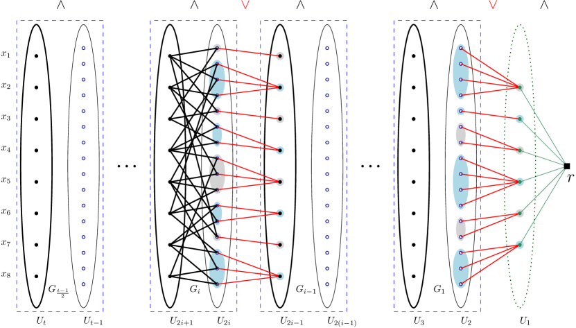
Figure 1: This figure provides a high-level construction of the hardness instance. The bipartite representation of $(t-1)/2$ graphs $G_{1},\cdots,G_{\frac{t-1}{2}}$ along with a target set $U_{1}$ form the layers of our instance of MMSA_t. Each $G_{i}$ is represented as a bipartite graph with two set of nodes $U_{2i}=V(G_{i})$ and $U_{2i+1}=E(G_{i})$ where there is an edge between $e\in U_{2i}$ and $v\in U_{2i+1}$ iff $v$ is one of the endpoints of $e$ in $G_{i}$ (these are the bold black edges and correspond to AND gates). Moreover, layers of different $G_{i}$ are glued together via a mapping of edge-nodes of $G_{i}$ (i.e, the vertices in $U_{2i}$) to vertex-nodes of $G_{i-1}$ (i.e., the vertices in $U_{2i-1}$) and $U_{1}$ is added to handle the connection for $G_{1}$. These intermediate edges are the red edges in this figure and correspond to OR gates.

Note that the total number of vertices is very strongly concentrated around $n^{2/(2-{\varepsilon})}\cdot(t-1)/2$. Let us denote $m=n^{2/(2-{\varepsilon})}\cdot(t-1)/2$. Since we think of $t$ as a constant, we will analyze the lower bound as a function of $m$ (the total number of vertices up to a constant factor). To that end, let us note that in all the graphs $G_{i}$, we have $n\approx m^{1-{\varepsilon}/2}$, and $p=n^{-(2-2{\varepsilon})/(2-{\varepsilon})}\approx m^{-(1-{\varepsilon})}$.

Proof sketch of integrality gap.

Let us begin by analyzing the optimum. We need to cover all $|U_{1}|\approx m^{1-{\varepsilon}}$ vertices in $U_{1}$, which forces us to choose that many vertices in $U_{2}$. Since each vertex in $U_{2}$ is connected to exactly two vertices in $U_{3}$ via AND gates, satisfying any choice of $|U_{1}|$ vertices in $U_{2}$ require at most $2|U_{1}|$ vertices in $U_{3}$. However, this is also a lower bound, since an arbitrary choice of $m^{1-{\varepsilon}}$ vertices in $U_{3}$ (corresponding to choosing $k_{1}=m^{1-{\varepsilon}}$ vertices in $G_{1}$) will result in a subgraph with expected number of edges $pk_{1}^{2}\approx m^{-(1-{\varepsilon})+2(1-{\varepsilon})}=m^{1-{\varepsilon}}$, and a Chernoff bound shows that no significantly smaller subgraph can have this many induced edges. This argument may be repeated now for all the subsequent layers, since each time we will end up with $\Omega(m^{1-{\varepsilon}})$ vertices in $U_{2i-1}$ that need to be satisfied, which forces us to choose that many vertices in $U_{2i}$ (since for any pair of vertices in $U_{2i-1}$, the number of their common neighbors in $U_{2i}$ is zero and the corresponding layer of $U_{2i}\rightarrow U_{2i-1}$ is an OR layer), and a subgraph with that many edges in $G_{i}$ must have $\Omega(m^{1-{\varepsilon}})$ vertices, which means that we will incur a set of at least this size in $U_{2i+1}$. Thus, the optimum is $\Theta(m^{1-{\varepsilon}})$.

Now let us see what fractional solution survives the basic SDP and Sherali-Adams. At first we know that for a goal of $k_{1}^{*}\geq\sqrt{n}$ vertices (in $U_{3}$, we have a fractional solution that represents as $k_{1}^{*}$-subgraph with $k_{1}^{*}\sqrt{pn}$ edges. Thus, to achieve our goal of fractional weight $m^{1-{\varepsilon}}$ in $U_{2}$ (representing edges in the subgraph in $G_{1}$), we need to choose $k_{1}^{*}$ such that $k_{1}^{*}\sqrt{pn}=m^{1-{\varepsilon}}$ which implies that $k_{1}^{*}\approx\frac{m^{1-{\varepsilon}}}{m^{-(1-{\varepsilon})/2+(2-{\varepsilon})/4}}=m^{1-5{\varepsilon}/4}$. Thus, in our fractional solution, LP weight $m^{1-5{\varepsilon}/4}$ is distributed evenly among the vertices of $U_{3}$. We can repeat this argument, showing that $U_{2i-1}$ has LP weight $\approx m^{1-(3+i){\varepsilon}/4}$ and that to get an fractional solution with this edge weight in $G_{i}$, it suffices to set the fractional vertex weight to $k^{*}_{i}=m^{1-(4+i){\varepsilon}/4}$, as long as $k^{*}_{i}\geq\sqrt{n}$. That is, as long as $m^{1-(4+i){\varepsilon}/4}\geq m^{(2-{\varepsilon})/4}$ which corresponds to $i\leq\frac{2}{{\varepsilon}}-3$. Once $i\geq\frac{2}{{\varepsilon}}-3$, we can use the log-density lower bound for obtaining fractional edge weight $k^{*}_{i-1}=m^{1-(3+i)/4}$, which sets the fractional vertex weight to $k^{*}_{i}=m^{2\alpha_{i}/(1-2{\varepsilon})}\approx n^{\alpha_{i}}$ such that

$$m^{1-(3+i){\varepsilon}/4}=k^{*}_{i}n^{\alpha_{i}\beta}=k_{i}^{*}n^{\alpha_{i}\cdot{\varepsilon}/(2-{\varepsilon})}\approx n^{\alpha_{i}}n^{\alpha_{i}\cdot{\varepsilon}/(2-{\varepsilon})}=n^{2\alpha_{i}/(2-{\varepsilon})}\approx m^{\alpha_{i}}.$$

Recall that this bound holds as long as $\alpha_{i}\leq 1/2$. Indeed, at this point, since $i\geq\frac{2}{{\varepsilon}}-3$, we get $\alpha_{i}=1-\frac{(3+i){\varepsilon}}{4}\leq 1-\frac{2}{4}=\frac{1}{2}$. From this point on, the sequence of $k^{*}_{i}$ keeps decreasing, so it is always at most $\sqrt{n}$, and we can always use the log-density lower bound.

We now follow a similar calculation. If the relaxation places fractional weight $k^{*}_{i-1}=m^{\delta_{i-1}}$ on $U_{2i-1}$, then to get this fractional edge weight in $G_{i}$, we need fractional vertex weight $k^{*}_{i}=n^{\alpha_{i}}$ such that $m^{\delta_{i-1}}\approx n^{2\alpha_{i}/(2-{\varepsilon})}\approx m^{\alpha_{i}}$, and so the fractional weight on $U_{2i+1}$ will be $k^{*}_{i}=n^{\delta_{i-1}}=m^{\delta_{i-1}\cdot(2-{\varepsilon})/2}$. Thus, we get a decrease of a factor of $(2-{\varepsilon})/2$ in the exponent at each step, and an additional $\log(1/(2{\varepsilon}))/\log(2/(2-{\varepsilon}))$ steps will bring us down to $m^{{\varepsilon}}$. Thus, the integrality gap is at least $m^{1-2{\varepsilon}}$ for MMSA_t for any $t\geq\frac{2}{{\varepsilon}}-3+\frac{\log(1/(2{\varepsilon}))}{\log(2/(2-{\varepsilon}))}$. Thus the integrality gap does tend to linear as $t$ increases, with a dependence which is at most $t=O((1/{\varepsilon})\log(1/{\varepsilon}))$, or in other words, an integrality gap of $m^{1-O((\log t)/t)}$.

Appendix A Adapting and Applying our Algorithm to Partial Red-Blue Set Cover

Let us now consider the variation in which we are given a parameter $\hat{k}$, and are only required to cover at least $\hat{k}$ elements in a feasible solution. The algorithm and analysis work with almost no change other than the following.

In the algorithm, the stopping condition of the loop is of course no longer once we have covered all blue elements, but once we have covered at least $\hat{k}$ of them.

A slightly more subtle change involves the analysis of the LP rounding in the final iteration. The notion of progress towards a certain approximation guarantee may not be valid if the ratio of red elements to blue elements covered is still as small as required, but the number of blue elements added is far more than we need. Rather than derandomize the rounding, one can show that it succeeds (despite this issue) with high probability. Let us briefly sketch the argument here.

First, note that we can always preemptively discard any sets with more than $\mathrm{OPT}$ red elements, and so we may assume that $r_{\alpha}\leq\mathrm{OPT}$. Suppose we need to cover an additional $k^{*}$ elements in order to reach the target of $\hat{k}$ blue elements total. Since our bound on $\mathbb{E}[|\Gamma_{R_{\alpha}}(J^{*})|]$ is a linear function of our bound on $\mathbb{E}[|J^{*}\setminus J_{+}|]$, by a Chernoff bound we have $|\Gamma_{R_{\alpha}}(J^{*})|=\tilde{O}(r_{\alpha}A)$ with all but exponentially small probability. On the other hand, $|\Gamma_{B}(J^{*})|$ is always at most $|B|$, so by Markov, we have

$$\mathrm{Prob}\left[|\Gamma_{B}(J^{*})|\leq\frac{\mathbb{E}[|\Gamma_{B}(J^{*})|]}{2}\right]\leq\frac{|B|-\mathbb{E}[|\Gamma_{B}(J^{*})|]}{|B|-\mathbb{E}[|\Gamma_{B}(J^{*})|]/2}\leq 1-\frac{1}{2|B|}.$$

Thus, repeating the rounding a polynomial number of times (in a given iteration), with all but exponentially small probability we can find a set $\hat{J}\subseteq J$ that satisfies both

$$|\Gamma_{B}(\hat{J})|\geq\frac{\mathbb{E}[|\Gamma_{B}(J^{*})|]}{2}\qquad\text{and}\qquad|\Gamma_{R_{\alpha}}(\hat{J})|]=\tilde{O}(r_{\alpha}A).$$

Now if $\mathbb{E}[|\Gamma_{B}(J^{*})|]\leq 2k^{*}$, then we have the required ratio and bound on the number of new red elements by the previous analysis. If $\mathbb{E}[|\Gamma_{B}(J^{*})|]>2k^{*}$, then this will be the last iteration, as we will cover at least the required $k^{*}$ additional blue elements, and the number of red elements added at this final stage is at most $\tilde{O}(r_{\alpha}A)\leq\tilde{O}(A\cdot\mathrm{OPT})$, so we maintain the desired approximation ratio.

Appendix B Additional LP Constraints for MMSA₄

The following is a complete list of lifted constraints that we use in addition to the basic LP relaxation for MMSA₄:

$$X^{(h)}_{j}=X^{(j)}_{h} \forall j\in J,\forall h\in S$$

$$X^{(j)}_{j}=x_{j} \forall j\in J$$

$$\sum_{h\in\Gamma_{S}(i)}X_{h}^{(j)}\geq X_{i}^{(j)} \forall j\in J\forall i\in R$$

$$X_{j}^{(j)}\leq X_{i}^{(j)} \forall j\in J\forall i\in\Gamma_{R}(j)$$

$$0\leq X_{a}^{(j)}\leq x_{j} \forall j\in J\forall a\in\{j\}\cup R\cup S$$

$$\sum_{h^{\prime}\in S}w_{h^{\prime}}^{(h)}\leq\mathrm{OPT} \forall h\in S$$

$$\sum_{\ell\in B}X_{\ell}^{(h)}\geq|B|/(\log k\log m)w_{h} \forall h\in S$$

$$X_{\ell}^{(h)}\leq\sum_{j\in\Gamma_{J}(\ell)}X_{\ell,j}^{(h)}\leq 2e\ln(2k)X_{\ell}^{(h)} \forall h\in S\forall\ell\in B$$

$$\Delta X_{j}^{(h)}\leq\sum_{\ell\in\Gamma_{B}(j)}X_{\ell,j}^{(h)}\leq 2\Delta X_{j}^{(h)} \forall h\in S\forall j\in J$$

$$0\leq X_{\ell,j}^{(h)}\leq X_{j}^{(h)},X_{\ell}^{(h)}\leq w_{h} \forall h\in S\forall\ell\in B\forall j\in J$$

$$\sum_{h^{\prime}\in\Gamma_{S}(i)}X_{h^{\prime}}^{(h)}\geq X_{i}^{(h)} \forall h\in S\forall i\in R$$

$$X_{j}^{(h)}\leq X_{i}^{(h)} \forall h\in S\forall(j,i)\in E(J,R)$$

$$0\leq X_{a}^{(h)}\leq w_{h} \forall h\in S\forall a\in B\cup J\cup R\cup S$$

References

• Abidha and Ashok [2022] V. Abidha and P. Ashok. Red blue set cover problem on axis-parallel hyperplanes and other objects. arXiv preprint arXiv:2209.06661, 2022.
• Alekhnovich et al. [2001] M. Alekhnovich, S. Buss, S. Moran, and T. Pitassi. Minimum propositional proof length is np-hard to linearly approximate. The Journal of Symbolic Logic, 66(1):171–191, 2001.
• Ashok et al. [2017] P. Ashok, S. Kolay, and S. Saurabh. Multivariate complexity analysis of geometric red blue set cover. Algorithmica, 79(3):667–697, 2017.
• Awasthi et al. [2010] P. Awasthi, A. Blum, and O. Sheffet. Improved guarantees for agnostic learning of disjunctions. In Proceedings of the Conference on Learning Theory, pages 359–367, 2010.
• Carr et al. [2000] R. D. Carr, S. Doddi, G. Konjevod, and M. Marathe. On the red-blue set cover problem. In Proceedings of the Symposium on Discrete Algorithms, pages 345–353, 2000.
• Chan and Hu [2015] T. M. Chan and N. Hu. Geometric red–blue set cover for unit squares and related problems. Computational Geometry, 48(5):380–385, 2015.
• Charikar et al. [2016] M. Charikar, Y. Naamad, and A. Wirth. On approximating target set selection. In Proceedings of the International Workshop on Approximation, Randomization, and Combinatorial Optimization, 2016.
• Chlamtáč and Manurangsi [2018] E. Chlamtáč and P. Manurangsi. Sherali–Adams integrality gaps matching the log-density threshold. Approximation, Randomization, and Combinatorial Optimization. Algorithms and Techniques, 2018.
• Chlamtáč et al. [2016] E. Chlamtáč, M. Dinitz, C. Konrad, G. Kortsarz, and G. Rabanca. The densest $k$-subhypergraph problem. In Proceedings of the International Workshop on on Approximation, Randomization, and Combinatorial Optimization. Algorithms and Techniques, 2016.
• Chlamtáč et al. [2017] E. Chlamtáč, M. Dinitz, and Y. Makarychev. Minimizing the union: Tight approximations for small set bipartite vertex expansion. In Proceedings of the Symposium on Discrete Algorithms, pages 881–899, 2017.
• Dinur and Safra [2004] I. Dinur and S. Safra. On the hardness of approximating label-cover. Information Processing Letters, 89(5):247–254, 2004.
• Elkin and Peleg [2007] M. Elkin and D. Peleg. The hardness of approximating spanner problems. Theory of Computing Systems, 41(4):691–729, 2007.
• Goldwasser and Motwani [1997] M. Goldwasser and R. Motwani. Intractability of assembly sequencing: Unit disks in the plane. In Proceedings of WADS, volume 97, pages 307–320, 1997.
• Madireddy and Mudgal [2022] R. R. Madireddy and A. Mudgal. A constant–factor approximation algorithm for red–blue set cover with unit disks. Algorithmica, pages 1–33, 2022.
• Madireddy et al. [2021] R. R. Madireddy, S. C. Nandy, and S. Pandit. On the geometric red-blue set cover problem. In Proceedings of the International Workshop on Algorithms and Computation, pages 129–141, 2021.
• Miettinen [2008] P. Miettinen. On the positive–negative partial set cover problem. Information Processing Letters, 108(4):219–221, 2008.