Free Lunch for Domain Adversarial Training: Environment Label Smoothing

Yi-Fan Zhang1,2, Xue Wang3, Jian Liang1,2,
Zhang Zhang1,2, Liang Wang1,2, Rong Jin3, Tieniu Tan1,2
1National Laboratory of Pattern Recognition (NLPR), Institute of Automation
2School of Artificial Intelligence, University of Chinese Academy of Sciences (UCAS)
3 Machine Intelligence Technology, Alibaba Group
Work done during an internship at Alibaba Group.Work done at Alibaba Group, and now affiliated with Twitter.
Abstract

A fundamental challenge for machine learning models is how to generalize learned models for out-of-distribution (OOD) data. Among various approaches, exploiting invariant features by Domain Adversarial Training (DAT) received widespread attention. Despite its success, we observe training instability from DAT, mostly due to over-confident domain discriminator and environment label noise. To address this issue, we proposed Environment Label Smoothing (ELS), which encourages the discriminator to output soft probability, which thus reduces the confidence of the discriminator and alleviates the impact of noisy environment labels. We demonstrate, both experimentally and theoretically, that ELS can improve training stability, local convergence, and robustness to noisy environment labels. By incorporating ELS with DAT methods, we are able to yield the state-of-art results on a wide range of domain generalization/adaptation tasks, particularly when the environment labels are highly noisy. The code is avaliable at https://github.com/yfzhang114/Environment-Label-Smoothing.

1 Introduction

Despite being empirically effective on visual recognition benchmarks (Russakovsky et al., 2015), modern neural networks are prone to learning shortcuts that stem from spurious correlations (Geirhos et al., 2020), resulting in poor generalization for out-of-distribution (OOD) data. A popular thread of methods, minimizing domain divergence by Domain Adversarial Training (DAT) (Ganin et al., 2016), has shown better domain transfer performance, suggesting that it is potential to be an effective candidate to extract domain-invariant features. Despite its power for domain adaptation and domain generalization, DAT is known to be difficult to train and converge (Roth et al., 2017; Jenni & Favaro, 2019; Arjovsky & Bottou, 2017; Sønderby et al., 2016).
Refer to caption
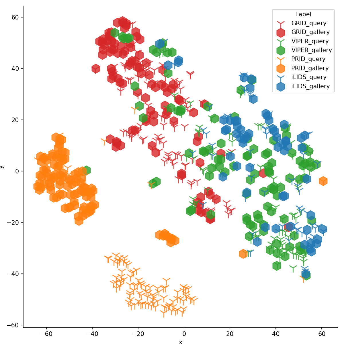
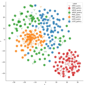
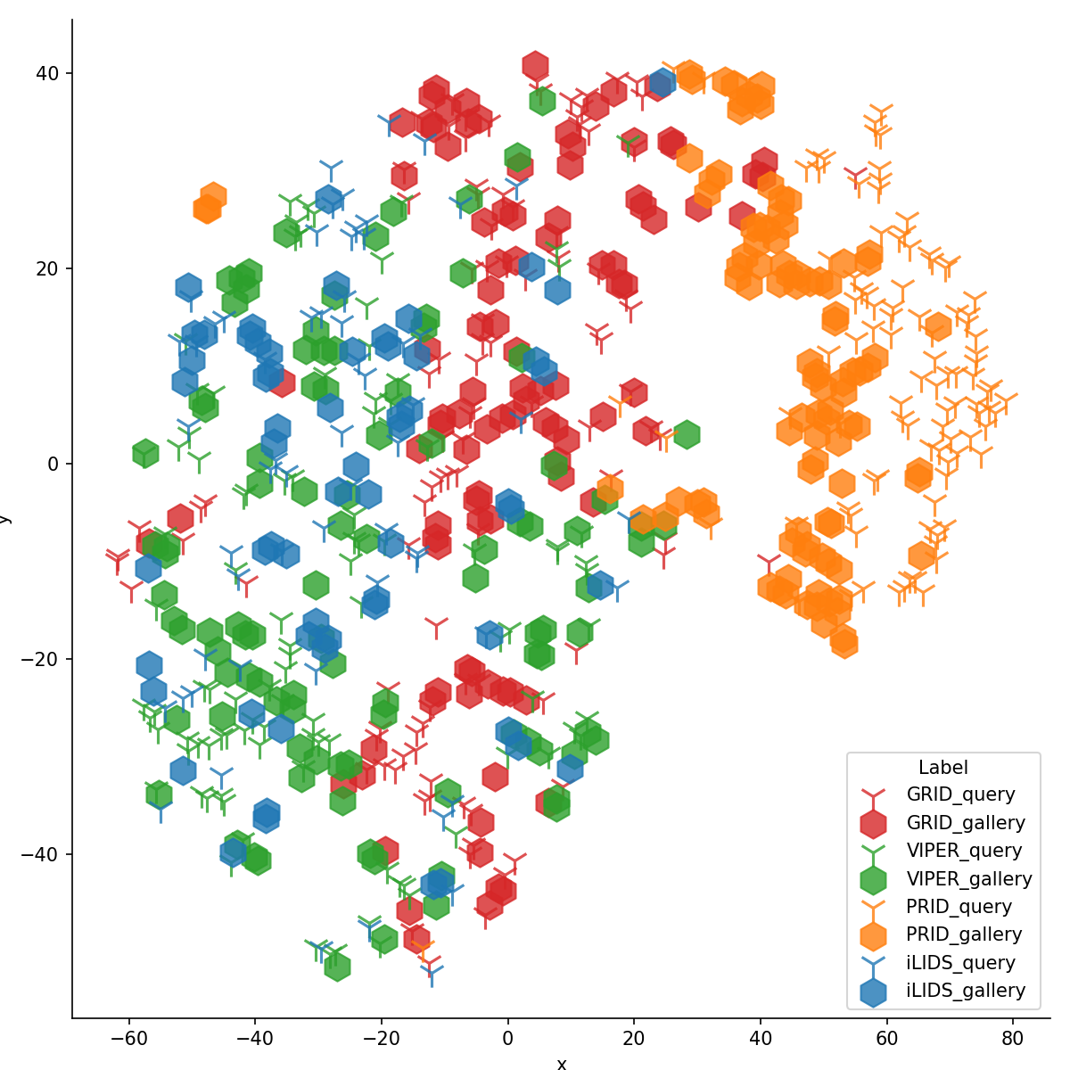
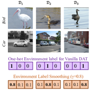
Figure 1: A motivating example of ELS with 3 domains on the VLCS dataset.

The main difficulty for stable training is to maintain healthy competition between the encoder and the domain discriminator. Recent work seeks to attain this goal by designing novel optimization methods (Acuna et al., 2022; Rangwani et al., 2022), however, most of them require additional optimization steps and slow the convergence. In this work, we aim to tackle the challenge from a totally different aspect from previous works, i.e., the environment label design.

Two important observations that lead to the training instability of DAT motivate this work: (i) The environment label noise from environment partition (Creager et al., 2021) and training (Thanh-Tung et al., 2019). As shown in Figure 1, different domains of the VLCS benchmark have no significant difference in image style and some images are indistinguishable for which domain they belong. Besides, when the encoder gets better, the generated features from different domains are more similar. However, regardless of their quality, features are still labeled differently. As shown in (Thanh-Tung et al., 2019; Brock et al., 2019), discriminators will overfit these mislabelled examples and then has poor generalization capability. (ii) To our best knowledge, DAT methods all assign one-hot environment labels to each data sample for domain discrimination, where the output probabilities will be highly confident. For DAT, a very confident domain discriminator leads to highly oscillatory gradients (Arjovsky & Bottou, 2017; Mescheder et al., 2018), which is harmful to training stability. The first observation inspires us to force the training process to be robust with regard to environment-label noise, and the second observation encourages the discriminator to estimate soft probabilities rather than confident classification. To this end, we propose Environment Label Smoothing (ELS), which is a simple method to tackle the mentioned obstacles for DAT. Next, we summarize the main methodological, theoretical, and experimental contributions.

Methodology: To our best knowledge, this is the first work to smooth environment labels for DAT. The proposed ELS yields three main advantages: (i) it does not require any extra parameters and optimization steps and yields faster convergence speed, better training stability, and more robustness to label noise theoretically and empirically; (ii) despite its efficiency, ELS is also easily to implement. People can easily incorporate ELS with any DAT methods in very few lines of code; (iii) ELS equipped DAT methods attain superior generalization performance compared to their native counterparts;

Theories: The benefit of ELS is theoretically verified in the following aspects. (i) Training stability. We first connect DAT to Jensen–Shannon/Kullback–Leibler divergence minimization, where ELS is shown able to extend the support of training distributions and relieve both the oscillatory gradients and gradient vanishing phenomenons, which results in stable and well-behaved training. (ii) Robustness to noisy labels. We theoretically verify that the negative effect caused by noisy labels can be reduced or even eliminated by ELS with a proper smooth parameter. (iii) Faster non-asymptotic convergence speed. We analyze the non-asymptotic convergence properties of DANN. The results indicate that incorporating with ELS can further speed up the convergence process. In addition, we also provide the empirical gap and analyze some commonly used DAT tricks.

Experiments: (i) Experiments are carried out on various benchmarks with different backbones, including image classification, image retrieval, neural language processing, genomics data, graph, and sequential data. ELS brings consistent improvement when incorporated with different DAT methods and achieves competitive or SOTA performance on various benchmarks, e.g., average accuracy on Rotating MNIST (52.1%62.1%percent52.1percent62.152.1\%\rightarrow 62.1\%), worst group accuracy on CivilComments (61.7%65.9%percent61.7percent65.961.7\%\rightarrow 65.9\%), test ID accuracy on RxRx1 (22.9%26.7%percent22.9percent26.722.9\%\rightarrow 26.7\%), average accuracy on Spurious-Fourier dataset (11.1%15.6%percent11.1percent15.611.1\%\rightarrow 15.6\%). (ii) Even if the environment labels are random or partially known, the performance of ELS + DANN will not degrade much and is superior to native DANN. (iii) Abundant analyzes on training dynamics are conducted to verify the benefit of ELS empirically. (iv) We conduct thorough ablations on hyper-parameter for ELS and some useful suggestions about choosing the best smooth parameter considering the dataset information are given.

2 Methodology

For domain generalization tasks, there are M𝑀M source domains {𝒟i}i=1Msuperscriptsubscriptsubscript𝒟𝑖𝑖1𝑀\{\mathcal{D}_{i}\}_{i=1}^{M}. Let the hypothesis hh be the composition of h=h^g^𝑔h=\hat{h}\circ g, where g𝒢𝑔𝒢g\in\mathcal{G} pushes forward the data samples to a representation space 𝒵𝒵\mathcal{Z} and h^=(h^1(),,h^M())^:𝒵[0,1]M;i=1Mh^i()=1:^subscript^1subscript^𝑀^formulae-sequence𝒵superscript01𝑀superscriptsubscript𝑖1𝑀subscript^𝑖1\hat{h}=(\hat{h}_{1}(\cdot),\dots,\hat{h}_{M}(\cdot))\in\hat{\mathcal{H}}:\mathcal{Z}\rightarrow[0,1]^{M};\sum_{i=1}^{M}\hat{h}_{i}(\cdot)=1 is the domain discriminator with softmax activation function. The classifier is defined as h^^:𝒵[0,1]C;i=1Ch^i()=1:superscript^^superscriptformulae-sequence𝒵superscript01𝐶superscriptsubscript𝑖1𝐶subscriptsuperscript^𝑖1\hat{h}^{\prime}\in\hat{\mathcal{H}^{\prime}}:\mathcal{Z}\rightarrow[0,1]^{C};\sum_{i=1}^{C}\hat{h}^{\prime}_{i}(\cdot)=1, where C𝐶C is the number of classes. The cost used for the discriminator can be defined as:

maxh^^dh^,g(𝒟1,,𝒟M)=maxh^𝔼𝐱𝒟1logh^1g(𝐱)++𝔼𝐱𝒟Mlogh^Mg(𝐱),subscript^^subscript𝑑^𝑔subscript𝒟1subscript𝒟𝑀subscript^subscript𝔼𝐱subscript𝒟1subscript^1𝑔𝐱subscript𝔼𝐱subscript𝒟𝑀subscript^𝑀𝑔𝐱\max_{\hat{h}\in\hat{\mathcal{H}}}d_{\hat{h},g}(\mathcal{D}_{1},\dots,\mathcal{D}_{M})=\max_{\hat{h}\in{\mathcal{H}}}\mathbb{E}_{\mathbf{x}\in\mathcal{D}_{1}}\log\hat{h}_{1}\circ g(\mathbf{x})+\dots+\mathbb{E}_{\mathbf{x}\in\mathcal{D}_{M}}\log\hat{h}_{M}\circ g(\mathbf{x}), (1)

where h^ig(𝐱)subscript^𝑖𝑔𝐱\hat{h}_{i}\circ g(\mathbf{x}) is the prediction probability that 𝐱𝐱\mathbf{x} is belonged to 𝒟isubscript𝒟𝑖\mathcal{D}_{i}. Denote y𝑦y the class label, then the overall objective of DAT is

minh^,gmaxh^1Mi=1M𝔼𝐱𝒟i[(h^g(𝐱),y)]+λdh^,g(𝒟1,,𝒟M),subscriptsuperscript^𝑔subscript^1𝑀superscriptsubscript𝑖1𝑀subscript𝔼𝐱subscript𝒟𝑖delimited-[]superscript^𝑔𝐱𝑦𝜆subscript𝑑^𝑔subscript𝒟1subscript𝒟𝑀\min_{\hat{h}^{\prime},g}\max_{\hat{h}}\frac{1}{M}\sum_{i=1}^{M}\mathbb{E}_{\mathbf{x}\in\mathcal{D}_{i}}[\ell(\hat{h}^{\prime}\circ g(\mathbf{x}),y)]+\lambda d_{\hat{h},g}(\mathcal{D}_{1},\dots,\mathcal{D}_{M}), (2)

where \ell is the cross-entropy loss for classification tasks and MSE for regression tasks, and λ𝜆\lambda is the tradeoff weight. We call the first term empirical risk minimization (ERM) part and the second term adversarial training (AT) part. Applying ELS, the target in Equ. (1) can be reformulated as

maxh^^dh^,g,γ(𝒟1,,𝒟M)=maxh^^𝔼𝐱𝒟1subscript^^subscript𝑑^𝑔𝛾subscript𝒟1subscript𝒟𝑀subscript^^subscript𝔼𝐱subscript𝒟1\displaystyle\max_{\hat{h}\in\hat{\mathcal{H}}}d_{\hat{h},g,\gamma}(\mathcal{D}_{1},\dots,\mathcal{D}_{M})=\max_{\hat{h}\in\hat{\mathcal{H}}}\mathbb{E}_{\mathbf{x}\in\mathcal{D}_{1}} [γlogh^1g(𝐱)+(1γ)M1j=1;j1Mlog(h^jg(𝐱))]++delimited-[]𝛾subscript^1𝑔𝐱1𝛾𝑀1superscriptsubscriptformulae-sequence𝑗1𝑗1𝑀subscript^𝑗𝑔𝐱limit-from\displaystyle\left[\gamma\log\hat{h}_{1}\circ g(\mathbf{x})+\frac{(1-\gamma)}{M-1}\sum_{j=1;j\neq 1}^{M}\log\left(\hat{h}_{j}\circ g(\mathbf{x})\right)\right]+\dots+ (3)
𝔼𝐱𝒟M[γlogh^Mg(𝐱)+(1γ)M1j=1;jMMlog(h^jg(𝐱))].subscript𝔼𝐱subscript𝒟𝑀delimited-[]𝛾subscript^𝑀𝑔𝐱1𝛾𝑀1superscriptsubscriptformulae-sequence𝑗1𝑗𝑀𝑀subscript^𝑗𝑔𝐱\displaystyle\mathbb{E}_{\mathbf{x}\in\mathcal{D}_{M}}\left[\gamma\log\hat{h}_{M}\circ g(\mathbf{x})+\frac{(1-\gamma)}{M-1}\sum_{j=1;j\neq M}^{M}\log\left(\hat{h}_{j}\circ g(\mathbf{x})\right)\right].

3 Theoretical validation

In this section, we first assume the discriminator is optimized with no constraint, providing a theoretical interpretation of applying ELS. Then how ELS makes the training process more stable is discussed based on the interpretation and some analysis of the gradients. We next theoretically show that with ELS, the effect of label noise can be eliminated. Finally, to mitigate the impact of the no constraint assumption, the empirical gap, parameterization gap, and non-asymptotic convergence property are analyzed respectively. All omitted proofs can be found in the Appendix.

3.1 Divergence Minimization Interpretation

In this subsection, the connection between ELS/one-sided ELS and divergence minimization is studied. The advantages brought by ELS and why GANs prefer one-sided ELS are theoretically claimed. We begin with the two-domain setting, which is used in domain adaptation and generative adversarial networks. Then the result in the multi-domain setting is further developed.

Proposition 1.

Given two domain distributions 𝒟S,𝒟Tsubscript𝒟𝑆subscript𝒟𝑇\mathcal{D}_{S},\mathcal{D}_{T} over X𝑋X, and a hypothesis class \mathcal{H}. We suppose h^^^^\hat{h}\in\hat{\mathcal{H}} the optimal discriminator with no constraint, denote the mixed distributions with hyper-parameter γ[0.5,1]𝛾0.51\gamma\in[0.5,1] as {𝒟S=γ𝒟S+(1γ)𝒟T𝒟T=γ𝒟T+(1γ)𝒟Scasessubscript𝒟superscript𝑆𝛾subscript𝒟𝑆1𝛾subscript𝒟𝑇subscript𝒟superscript𝑇𝛾subscript𝒟𝑇1𝛾subscript𝒟𝑆\left\{\begin{array}[]{c}\mathcal{D}_{S^{\prime}}=\gamma\mathcal{D}_{S}+(1-\gamma)\mathcal{D}_{T}\\ \mathcal{D}_{T^{\prime}}=\gamma\mathcal{D}_{T}+(1-\gamma)\mathcal{D}_{S}\\ \end{array}\right.. Then minimizing domain divergence by adversarial training with ELS is equal to minimizing 2DJS(𝒟S||𝒟T)2log22D_{JS}(\mathcal{D}_{S^{\prime}}||\mathcal{D}_{T^{\prime}})-2\log 2, where DJSsubscript𝐷𝐽𝑆D_{JS} is the Jensen-Shanon (JS) divergence.

Compared to Proposition 2 in (Acuna et al., 2021) that adversarial training in DANN is equal to minimize 2DJS(𝒟S||𝒟T)2log22D_{JS}(\mathcal{D}_{S}||\mathcal{D}_{T})-2\log 2. The only difference here is the mixed distributions 𝒟S,𝒟Tsubscript𝒟superscript𝑆subscript𝒟superscript𝑇\mathcal{D}_{S^{\prime}},\mathcal{D}_{T^{\prime}}, which allows more flexible control on divergence minimization. For example, when γ=1𝛾1\gamma=1, 𝒟S=𝒟S,𝒟T=𝒟Tformulae-sequencesubscript𝒟superscript𝑆subscript𝒟𝑆subscript𝒟superscript𝑇subscript𝒟𝑇\mathcal{D}_{S^{\prime}}=\mathcal{D}_{S},\mathcal{D}_{T^{\prime}}=\mathcal{D}_{T} which is the same as the original adversarial training; when γ=0.5𝛾0.5\gamma=0.5, 𝒟S=𝒟T=0.5(𝒟S+𝒟T)subscript𝒟superscript𝑆subscript𝒟superscript𝑇0.5subscript𝒟𝑆subscript𝒟𝑇\mathcal{D}_{S^{\prime}}=\mathcal{D}_{T^{\prime}}=0.5(\mathcal{D}_{S}+\mathcal{D}_{T}) and DJS(𝒟S||𝒟T)=0D_{JS}(\mathcal{D}_{S^{\prime}}||\mathcal{D}_{T^{\prime}})=0, which means that this term will not supply gradients during training and the training process will convergence like ERM. In other words, γ𝛾\gamma controls the tradeoff between algorithm convergence and adversarial divergence minimization. One main argue that adjusting the tradeoff weight λ𝜆\lambda can also balance AT and ERM, however, λ𝜆\lambda can only adjust the gradient contribution of AT part, i.e., 2λDJS(𝒟S,𝒟T)2𝜆subscript𝐷𝐽𝑆subscript𝒟𝑆subscript𝒟𝑇2\lambda\nabla D_{JS}(\mathcal{D}_{S},\mathcal{D}_{T}) and cannot affect the training dynamic of DJS(𝒟S,𝒟T)subscript𝐷𝐽𝑆subscript𝒟𝑆subscript𝒟𝑇D_{JS}(\mathcal{D}_{S},\mathcal{D}_{T}). For example, when 𝒟S,𝒟Tsubscript𝒟𝑆subscript𝒟𝑇\mathcal{D}_{S},\mathcal{D}_{T} have disjoint support, DJS(𝒟S,𝒟T)subscript𝐷𝐽𝑆subscript𝒟𝑆subscript𝒟𝑇\nabla D_{JS}(\mathcal{D}_{S},\mathcal{D}_{T}) is always zero no matter what λ𝜆\lambda is given. On the contrary, the proposed technique smooths the optimization distribution 𝒟S,𝒟Tsubscript𝒟𝑆subscript𝒟𝑇\mathcal{D}_{S},\mathcal{D}_{T} of AT, making the whole training process more stable, but controlling λ𝜆\lambda cannot do. In the experimental section, we show that in some benchmarks, the model cannot converge even if the tradeoff weight is small enough, however, when ELS is applied, DANN+ELS attains superior results and without the need for small tradeoff weights or small learning rate.

As shown in (Goodfellow, 2016), GANs always use a technique called one-sided label smoothing, which is a simple modification of the label smoothing technique and only replaces the target for real examples with a value slightly less than one, such as 0.9. Here we connect one-sided label smoothing to JS divergence and seek the difference between native and one-sided label smoothing techniques. See Appendix A.2 for proof and analysis. We further extend the above theoretical analysis to multi-domain settings, e.g., domain generalization, and multi-source GANs (Trung Le et al., 2019) (See Proposition 3 in Appendix A.3 for detailed proof and analysis.). We find that with ELS, a flexible control on algorithm convergence and divergence minimization tradeoffs can be attained.

3.2 Training Stability

Noise injection for extending distribution supports. The main source of training instability of GANs is the real and the generated distributions have disjoint supports or lie on low dimensional manifolds (Arjovsky & Bottou, 2017; Roth et al., 2017). Adding noise from an arbitrary distribution to the data is shown to be able to extend the support of both distributions (Jenni & Favaro, 2019; Arjovsky & Bottou, 2017; Sønderby et al., 2016) and will protect the discriminator against measure 0 adversarial examples (Jenni & Favaro, 2019), which result in stable and well-behaved training. Environment label smoothing can be viewed as a kind of noise injection, e.g., in Proposition 1, 𝒟S=𝒟T+γ(𝒟S𝒟T)subscript𝒟superscript𝑆subscript𝒟𝑇𝛾subscript𝒟𝑆subscript𝒟𝑇\mathcal{D}_{S^{\prime}}=\mathcal{D}_{T}+\gamma(\mathcal{D}_{S}-\mathcal{D}_{T}) where the noise is γ(𝒟S𝒟T)𝛾subscript𝒟𝑆subscript𝒟𝑇\gamma(\mathcal{D}_{S}-\mathcal{D}_{T}) and the two distributions will be more likely to have joint supports.

ELS relieves the gradient vanishing phenomenon. As shown in Section 3.1, the adversarial target is approximating KL or JS divergence, and when the discriminator is not optimal, a such approximation is inaccurate. We show that in vanilla DANN, as the discriminator gets better, the gradient passed from discriminator to the encoder vanishes (Proposition 25 and Proposition 32). Namely, either the approximation is inaccurate, or the gradient vanishes, which will make adversarial training extremely hard (Arjovsky & Bottou, 2017). Incorporating ELS is shown able to relieve the
Refer to caption
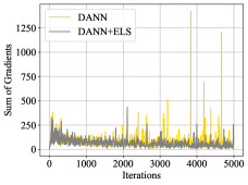
Figure 2: The sum of gradients provided to the encoder by the adversarial loss.

gradient vanishing phenomenon when the discriminator is close to the optimal one and stabilizes the training process.

ELS serves as a data-driven regularization and stabilizes the oscillatory gradients. Gradients of the encoder with respect to adversarial loss remain highly oscillatory in native DANN, which is an important reason for the instability of adversarial training (Mescheder et al., 2018). Figure 2 shows the gradient dynamics throughout the training process, where the PACS dataset is used as an example. With ELS, the gradient brought by the adversarial loss is smoother and more stable. The benefit is theoretically supported in Section A.6, where applying ELS is shown similar to adding a regularization term on discriminator parameters, which stabilizes the supplied gradients compared to the vanilla adversarial loss.

3.3 ELS meets noisy labels

To analyze the benefits of ELS when noisy labels exist, we adopt the symmetric noise model (Kim et al., 2019). Specifically, given two environments with a high-dimensional feature x𝑥x and environment label y{0,1}𝑦01y\in\{0,1\}, assume that noisy labels y~~𝑦\tilde{y} are generated by random noise transition with noise rate e=P(y~=1|y=0)=P(y~=0|y=1)𝑒𝑃~𝑦conditional1𝑦0𝑃~𝑦conditional0𝑦1e=P(\tilde{y}=1|y=0)=P(\tilde{y}=0|y=1). Denote f:=h^gassign𝑓^𝑔f:=\hat{h}\circ g, \ell the cross-entropy loss and y~γsuperscript~𝑦𝛾\tilde{y}^{\gamma} the smoothed noisy label, then minimizing the smoothed loss with noisy labels can be converted to

minf𝔼(x,y~)𝒟~[(f(x),y~γ)]=minf𝔼(x,y~)𝒟~[γ(f(x),y~)+(1γ)(f(x),1y~)]subscript𝑓subscript𝔼similar-to𝑥~𝑦~𝒟delimited-[]𝑓𝑥superscript~𝑦𝛾subscript𝑓subscript𝔼similar-to𝑥~𝑦~𝒟delimited-[]𝛾𝑓𝑥~𝑦1𝛾𝑓𝑥1~𝑦\displaystyle\min_{f}\mathbb{E}_{(x,\tilde{y})\sim\tilde{\mathcal{D}}}[\ell(f(x),\tilde{y}^{\gamma})]=\min_{f}\mathbb{E}_{(x,\tilde{y})\sim\tilde{\mathcal{D}}}\left[\gamma\ell(f(x),\tilde{y})+(1-\gamma)\ell(f(x),1-\tilde{y})\right] (4)
=minf𝔼(x,y)𝒟[(f(x),yγ)]+(γγe+2γe)𝔼(x,y)𝒟[(f(x),1y)(f(x),y)]absentsubscript𝑓subscript𝔼similar-to𝑥𝑦𝒟delimited-[]𝑓𝑥superscript𝑦superscript𝛾superscript𝛾𝛾𝑒2𝛾𝑒subscript𝔼similar-to𝑥𝑦𝒟delimited-[]𝑓𝑥1𝑦𝑓𝑥𝑦\displaystyle=\min_{f}\mathbb{E}_{(x,y)\sim\mathcal{D}}[\ell(f(x),y^{\gamma^{*}})]+(\gamma^{*}-\gamma-e+2\gamma e)\mathbb{E}_{(x,y)\sim\mathcal{D}}[\ell(f(x),1-y)-\ell(f(x),y)]

where γsuperscript𝛾\gamma^{*} is the optimal smooth parameter that makes the classifier return the best performance on unseen clean data (Wei et al., 2022). The first term in Equ. (4) is the risk under the clean label. The influence of both noisy labels and ELS are reflected in the last term of the Equ. (4). 𝔼(x,y)𝒟[(f(x),1y)(f(x),y)]subscript𝔼similar-to𝑥𝑦𝒟delimited-[]𝑓𝑥1𝑦𝑓𝑥𝑦\mathbb{E}_{(x,y)\sim\mathcal{D}}[\ell(f(x),1-y)-\ell(f(x),y)] is the opposite of the optimization process as we expect. Without label smoothing, the weight will be γ1+esuperscript𝛾1𝑒\gamma^{*}-1+e and a high noisy rate e𝑒e will let this harmful term contributes more to our optimization. On the contrary, by choosing a smooth parameter γ=γe12e𝛾superscript𝛾𝑒12𝑒\gamma=\frac{\gamma^{*}-e}{1-2e}, the second term will be removed. For example, if e=0𝑒0e=0, the best smooth parameter is just γsuperscript𝛾\gamma^{*}.

3.4 Empirical Gap and Parameterization Gap

Propositions in Section 3.1 and Section 3.2 are based on two unrealistic assumptions. (i) Infinite data samples, and (ii) the discriminator is optimized without a constraint, namely, the discriminator is optimized over infinite-dimensional space. In practice, only empirical distributions with finite samples are observed and the discriminator is always constrained to smaller classes such as neural networks (Goodfellow et al., 2014) or reproducing kernel Hilbert spaces (RKHS) (Li et al., 2017a). Besides, as shown in (Arora et al., 2017; Schäfer et al., 2019), JS divergence has a large empirical gap, e.g., let 𝒟μ,𝒟νsubscript𝒟𝜇subscript𝒟𝜈\mathcal{D}_{\mu},\mathcal{D}_{\nu} be uniform Gaussian distributions 𝒩(0,1dI)𝒩01𝑑𝐼\mathcal{N}(0,\frac{1}{d}I), and 𝒟^μ,𝒟^νsubscript^𝒟𝜇subscript^𝒟𝜈\hat{\mathcal{D}}_{\mu},\hat{\mathcal{D}}_{\nu} be empirical versions of 𝒟μ,𝒟νsubscript𝒟𝜇subscript𝒟𝜈\mathcal{D}_{\mu},\mathcal{D}_{\nu} with n𝑛n examples. Then we have |dJS(𝒟μ,𝒟ν)dJS(𝒟^μ,𝒟^ν)|=log2subscript𝑑𝐽𝑆subscript𝒟𝜇subscript𝒟𝜈subscript𝑑𝐽𝑆subscript^𝒟𝜇subscript^𝒟𝜈2|d_{JS}(\mathcal{D}_{\mu},\mathcal{D}_{\nu})-d_{JS}(\hat{\mathcal{D}}_{\mu},\hat{\mathcal{D}}_{\nu})|=\log 2 with high probability. Namely, the empirical divergence cannot reflect the true distribution divergence.

A natural question arises: “Given finite samples to multi-domain AT over finite-dimensional parameterized space, whether the expectation over the empirical distribution converges to the expectation over the true distribution?”. In this subsection, we seek to answer this question by analyzing the empirical gap and parameterization gap, which is |dh^,g(𝒟1,,𝒟M)dh^,g(𝒟^1,,𝒟^M)|subscript𝑑^𝑔subscript𝒟1subscript𝒟𝑀subscript𝑑^𝑔subscript^𝒟1subscript^𝒟𝑀|d_{\hat{h},g}(\mathcal{D}_{1},\dots,\mathcal{D}_{M})-d_{\hat{h},g}(\hat{\mathcal{D}}_{1},\dots,\hat{\mathcal{D}}_{M})|, where D^isubscript^𝐷𝑖\hat{D}_{i} is the empirical distribution of 𝒟isubscript𝒟𝑖\mathcal{D}_{i} and h^^\hat{h} is constrained. We first show that, let \mathcal{H} be a hypothesis class of VC dimension d𝑑d, then for any δ(0,1)𝛿01\delta\in(0,1), with probability at least 1δ1𝛿1-\delta, the gap is less than 4(dlog(2n)+log2/δ)/n4𝑑2superscript𝑛2𝛿superscript𝑛4\sqrt{({d\log(2n^{*})+\log{2}/{\delta}})/{n^{*}}}, where n=min(n1,,nM)superscript𝑛subscript𝑛1subscript𝑛𝑀n^{*}=\min(n_{1},\dots,n_{M}) and nisubscript𝑛𝑖n_{i} is the number of samples in 𝒟isubscript𝒟𝑖\mathcal{D}_{i} (Appendix A.8). The above analysis is based on \mathcal{H} divergence and the VC dimension; we further analyze the gap when the discriminator is constrained to the Lipschitz continuous and build a connection between the gap and the model parameters. Specifically, suppose that each h^isubscript^𝑖\hat{h}_{i} is L𝐿L-Lipschitz with respect to the parameters and use p𝑝p to denote the number of parameters of h^isubscript^𝑖\hat{h}_{i}. Then given a universal constant c𝑐c such that when ncpMlog(Lp/ϵ)/ϵsuperscript𝑛𝑐𝑝𝑀𝐿𝑝italic-ϵitalic-ϵn^{*}\geq{cpM\log(Lp/\epsilon)}/{\epsilon}, we have with probability at least 1exp(p)1𝑝1-\exp(-p), the gap is less than ϵitalic-ϵ\epsilon (Appendix A.9). Although the analysis cannot support the benefits of ELS, as far as we know, it is the first attempt to study the empirical and parameterization gap of multi-domain AT.

3.5 Non-Asymptotic Convergence

As mentioned in Section 3.4, the analysis in Section 3.1 and Section 3.2 assumes that the optimal discriminator can be obtained, which implies that both the hypothesis set has infinite modeling capacity and the training process can converge to the optimal result. If the objective of AT is convex-concave, then many works can support the global convergence behaviors (Nowozin et al., 2016; Yadav et al., 2017). However, the convex-concave assumption is too unrealistic to hold true (Nie & Patel, 2020; Nagarajan & Kolter, 2017), namely, the updates of DAT are no longer guaranteed to converge. In this section, we focus on the local convergence behaviors of DAT of points near the equilibrium. Specifically, we focus on the non-asymptotic convergence, which is shown able to more precisely reveal the convergence of the dynamic system than the asymptotic analysis (Nie & Patel, 2020).

We build a toy example to help us understand the convergence of DAT. Denote η𝜂\eta the learning rate, γ𝛾\gamma the parameter for ELS, and c𝑐c a constant. We conclude our theoretical results here (which are detailed in Appendix A.10): (1) Simultaneous Gradient Descent (GD) DANN, which trains the discriminator and encoder simultaneously, has no guarantee of the non-asymptotic convergence. (2) If we train the discriminator ndsubscript𝑛𝑑n_{d} times once we train the encoder nesubscript𝑛𝑒n_{e} times, the resulting alternating Gradient Descent (GD) DANN could converge with a sublinear convergence rate only when the η4ndnec𝜂4subscript𝑛𝑑subscript𝑛𝑒𝑐\eta\leq\frac{4}{\sqrt{n_{d}n_{e}}c}. Such results support the importance of alternating GD training, which is commonly used during DANN implementation (Gulrajani & Lopez-Paz, 2021). (3) Incorporate ELS into alternating GD DANN speed up the convergence rate by a factor 12γ112𝛾1\frac{1}{2\gamma-1}, that is, when η4ndnec12γ1𝜂4subscript𝑛𝑑subscript𝑛𝑒𝑐12𝛾1\eta\leq\frac{4}{\sqrt{n_{d}n_{e}}c}\frac{1}{2\gamma-1}, the model could converge.

Remark. In the above analysis, we made some assumptions e.g., in Section 3.5, we assume the algorithms are initialized in a neighborhood of a unique equilibrium point, and in Section 3.4 we assume that the NN is L-Lipschitz. These assumptions may not hold in practice, and they are computationally hard to verify. To this end, we empirically support our theoretical results, namely, verifying the benefits to convergence, training stability, and generalization results in the next section.

4 Experiments

To demonstrate the effectiveness of our ELS, in this section, we select a broad range of tasks (in Table 1), which are image classification, image retrieval, neural language processing, genomics, graph, and sequential prediction tasks. Our target is to include benchmarks with (i) various numbers of domains (from 333 to 120,084120084120,084); (ii) various numbers of classes (from 222 to 18,5301853018,530); (iii) various dataset sizes (from 3,20032003,200 to 448,000448000448,000); (iv) various dimensionalities and backbones (Transformer, ResNet, MobileNet, GIN, RNN). See Appendix C for full details of all experimental settings, including dataset details, hyper-parameters, implementation details, and model structures. We conduct all the experiments on a machine with i7-8700K, 32G RAM, and four GTX2080ti. All experiments are repeated 333 times with different seeds and the full experimental results can be found in the appendix.

Table 1: A summary on evaluation benchmarks. Wg. acc. denotes worst group accuracy, 10 %/ acc. denotes 10th percentile accuracy. GIN (Xu et al., 2018) denotes Graph Isomorphism Networks, and CRNN (Gagnon-Audet et al., 2022) denotes convolutional recurrent neural networks.

Task Dataset Domains Classes Metric Backbone # Data Examples Rotated MNIST 6 rotated angles 10 Avg. acc. MNIST ConvNet 70,000 PACS 4 image styles 7 Avg. acc. ResNet50 9,991 VLCS 4 image styles 5 Avg. acc. ResNet50 10,729 Office-31 3 image styles 31 Avg. acc. ResNet50/ResNet18 4,110 Office-Home 4 image styles 65 Avg. acc. ResNet50/ViT 15,500 Images Classification Rotating MNIST 8 rotated angles 10 Avg. acc. EncoderSTN 60,000 Image Retrieval MS 5 locations 18,530 mAP, Rank m𝑚m MobileNet×1.4absent1.4\times 1.4 121,738 CivilComments 8 demographic groups 2 Avg/Wg acc. DistillBERT 448,000 Neural Language Processing Amazon 7676 reviewers 5 10 %/Avg/Wg acc. DistillBERT 100,124 RxRx1 51 experimental batch 1139 Wg/Avg/Test ID acc. ResNet-50 125,510 Genomics and Graph OGB-MolPCBA 120,084 molecular scaffold 128 Avg. acc. GIN 437,929 Spurious-Fourier 3 spurious correlations 2 Avg. acc. LSTM 12,000 Sequential Prediction HHAR 5 smart devices 6 Avg. acc. Deep ConvNets 13,674

4.1 Numerical Results on Different Settings and Benchmarks

Domain Generalization and Domain Adaptation on Image Classification Tasks. We first incorporate ELS into SDAT, which is a variant of the DAT method and achieves the state-of-the-art performance on the Office-Home dataset. Table 2 and Table 4 show that with the simple smoothing trick, the performance of SDAT is consistently improved, and on many of the domain pairs, the improvement is greater than 1%percent11\%. Besides, the ELS can also bring consistent improvement both with ResNet-18, ResNet-50, and ViT backbones. The average domain generalization results on other benchmarks are shown in Table 3. We observe consistent improvements achieved by DANN+ELS compared to DANN and the average accuracy on VLCS achieved by DANN+ELS (81.5%percent81.581.5\%) clearly outperforms all other methods. See Appendix D.1 for Multi-Source Domain Generalization performance, DG performance on Rotated MNIST and on Image Retrieval benchmarks.

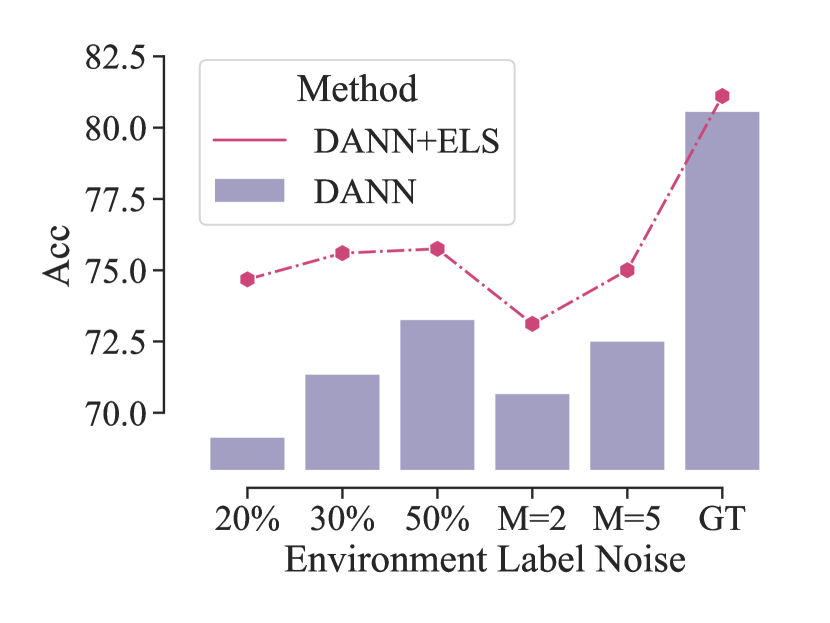
Domain Generalization with Partial Environment labels. One of the main advantages brought by ELS is the robustness to environment label noise. As shown in Figure 4, when all environment labels are known (GT), DANN+ELS is slightly better than DANN. When partial environment labels are known, for example, 30%percent3030\% means the environment labels of 30%percent3030\% training data are known and others are annotated differently than the ground truth annotations, DANN+ELS outperform DANN by a large margin (more than 5%percent55\% accuracy when only 20%percent2020\% correct environment labels are given). Besides, we further assume the total number of environments is also unknown and the environment number is generated randomly. M=2 in Figure 4 means we partition all the training data randomly into two domains, which are used for training then. With random environment partitions, DANN+ELS consistently beats DANN by a large margin, which verifies that the smoothness of the discrimination loss brings significant robustness to environment label noise for DAT.

Table 2: The domain adaptation accuracies (%) on Office-31. \uparrow denotes improvement of a method with ELS compared to that wo/ ELS.
A - W D - W W - D A - D D - A W - A Avg
ResNet18
ERM (Vapnik, 1999) 72.2 97.7 100.0 72.3 61.0 59.9 77.2
DANN (Ganin et al., 2016) 84.1 98.1 99.8 81.3 60.8 63.5 81.3
DANN+ELS 85.5 99.1 100.0 82.7 62.1 64.5 82.4
\uparrow 1.4 1.0 0.2 1.4 1.3 1.1 1.1
SDAT (Rangwani et al., 2022) 87.8 98.7 100.0 82.5 73.0 72.7 85.8
SDAT+ELS 88.9 99.3 100.0 83.9 74.1 73.9 86.7
\uparrow 1.1 0.5 0.0 1.4 1.1 1.2 0.9
ResNet50
ERM (Vapnik, 1999) 75.8 95.5 99.0 79.3 63.6 63.8 79.5
ADDA (Tzeng et al., 2017) 94.6 97.5 99.7 90.0 69.6 72.5 87.3
CDAN (Long et al., 2018) 93.8 98.5 100.0 89.9 73.4 70.4 87.7
MCC (Jin et al., 2020) 94.1 98.4 99.8 95.6 75.5 74.2 89.6
DANN (Ganin et al., 2016) 91.3 97.2 100.0 84.1 72.9 73.6 86.5
DANN++ELS 92.2 98.5 100.0 85.9 74.3 75.3 87.7
\uparrow 0.9 1.3 0.0 1.8 1.4 1.7 1.2
SDAT (Rangwani et al., 2022) 92.7 98.9 100.0 93.0 78.5 75.7 89.8
SDAT++ELS 93.6 99.0 100.0 93.4 78.7 77.5 90.4
\uparrow 0.9 0.1 0.0 0.4 0.2 1.8 0.6
Table 3: The domain generalization accuracies (%) on VLCS, and PACS. \uparrow denotes improvement of DANN+ELS compared to DANN.
Algorithm PACS VLCS
A C P S Avg C L S V Avg
ERM (Vapnik, 1999) 87.8 ± 0.4 82.8 ± 0.5 97.6 ± 0.4 80.4 ± 0.6 87.2 97.7 ± 0.3 65.2 ± 0.4 73.2 ± 0.7 75.2 ± 0.4 77.8
IRM (Arjovsky et al., 2019) 85.7 ± 1.0 79.3 ± 1.1 97.6 ± 0.4 75.9 ± 1.0 84.6 97.6 ± 0.5 64.7 ± 1.1 69.7 ± 0.5 76.6 ± 0.7 77.2
DANN (Ganin et al., 2016) 85.4 ±plus-or-minus\pm 1.2 83.1 ±plus-or-minus\pm 0.8 96.3 ±plus-or-minus\pm 0.4 79.6 ±plus-or-minus\pm 0.8 86.1 98.6 ±plus-or-minus\pm 0.8 73.2 ±plus-or-minus\pm 1.1 72.8 ±plus-or-minus\pm 0.8 78.8 ±plus-or-minus\pm 1.2 80.8
ARM (Zhang et al., 2021b) 85.0 ±plus-or-minus\pm 1.2 81.4 ±plus-or-minus\pm 0.2 95.9 ±plus-or-minus\pm 0.3 80.9 ±plus-or-minus\pm 0.5 85.8 97.6 ±plus-or-minus\pm 0.6 66.5 ±plus-or-minus\pm 0.3 72.7 ±plus-or-minus\pm 0.6 74.4 ±plus-or-minus\pm 0.7 77.8
Fisher (Rame et al., 2021) —— —— —— —— 86.9 —— —— —— —— 76.2
DDG (Zhang et al., 2021a) 88.9 ± 0.6 85.0 ± 1.9 97.2 ± 1.2 84.3 ± 0.7 88.9 99.1 ± 0.6 66.5 ± 0.3 73.3 ± 0.6 80.9 ± 0.6 80.0
DANN+ELS 87.8 ±plus-or-minus\pm 0.8 83.8 ±plus-or-minus\pm 1.6 97.1 ±plus-or-minus\pm 0.4 81.4 ±plus-or-minus\pm 1.3 87.5 99.1 ±plus-or-minus\pm 0.3 73.2 ±plus-or-minus\pm 1.1 73.8 ±plus-or-minus\pm 0.9 79.9 ±plus-or-minus\pm 0.9 81.5
\uparrow 2.4 0.7 0.8 1.8 1.4 0.5 0 1 1.1 0.7
Table 4: Accuracy (%percent\%) on Office-Home for unsupervised DA (with ResNet-50 and ViT backbone). SDAT++ELS outperforms other SOTA DA techniques and improves SDAT consistently.
Method Backbone A-C A-P A-R C-A C-P C-R P-A P-C P-R R-A R-C R-P Avg
ResNet-50 (He et al., 2016) 34.9 50.0 58.0 37.4 41.9 46.2 38.5 31.2 60.4 53.9 41.2 59.9 46.1
DANN (Ganin et al., 2016) 45.6 59.3 70.1 47.0 58.5 60.9 46.1 43.7 68.5 63.2 51.8 76.8 57.6
CDAN (Long et al., 2018) 49.0 69.3 74.5 54.4 66.0 68.4 55.6 48.3 75.9 68.4 55.4 80.5 63.8
MMD (Zhang et al., 2019) 54.9 73.7 77.8 60.0 71.4 71.8 61.2 53.6 78.1 72.5 60.2 82.3 68.1
f-DAL (Acuna et al., 2021) 56.7 77.0 81.1 63.1 72.2 75.9 64.5 54.4 81.0 72.3 58.4 83.7 70.0
SRDC (Tang et al., 2020) 52.3 76.3 81.0 69.5 76.2 78.0 68.7 53.8 81.7 76.3 57.1 85.0 71.3
SDAT (Rangwani et al., 2022) 57.8 77.4 82.2 66.5 76.6 76.2 63.3 57.0 82.2 75.3 62.6 85.2 71.8
SDAT++ELS 58.2 79.7 82.5 67.5 77.2 77.2 64.6 57.9 82.2 75.4 63.1 85.5 72.6
\uparrow ResNet-50 0.4 2.3 0.3 1.0 0.6 1.0 1.3 0.9 0.0 0.1 0.5 0.3 0.8
TVT (Yang et al., 2021) 74.9 86.6 89.5 82.8 87.9 88.3 79.8 71.9 90.1 85.5 74.6 90.6 83.6
CDAN (Long et al., 2018) 62.6 82.9 87.2 79.2 84.9 87.1 77.9 63.3 88.7 83.1 63.5 90.8 79.3
SDAT (Rangwani et al., 2022) 70.8 87.0 90.5 85.2 87.3 89.7 84.1 70.7 90.6 88.3 75.5 92.1 84.3
SDAT++ELS ViT 72.1 87.3 90.6 85.2 88.1 89.7 84.1 70.7 90.8 88.4 76.5 92.1 84.6
\uparrow 1.3 0.3 0.1 0.0 0.8 0.0 0.0 0.0 0.2 0.1 1.0 0.0 0.3

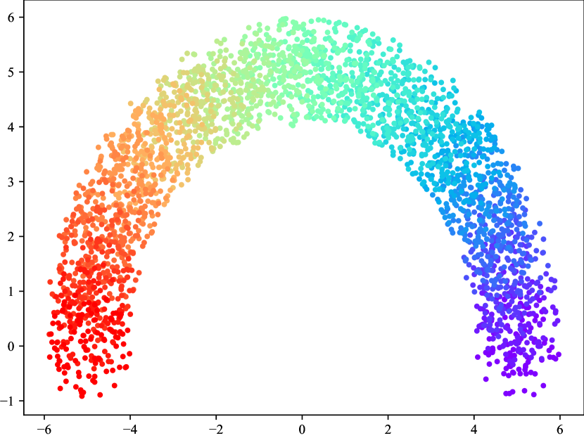
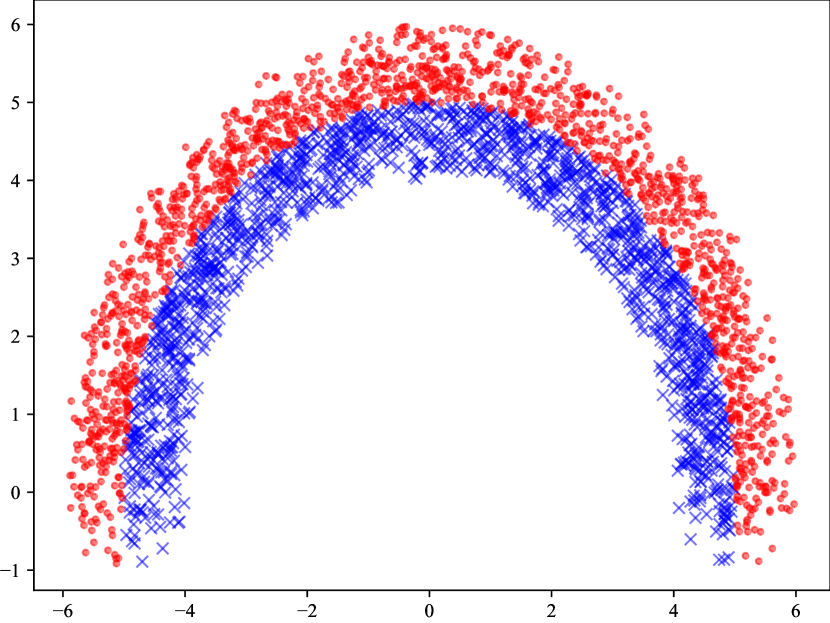
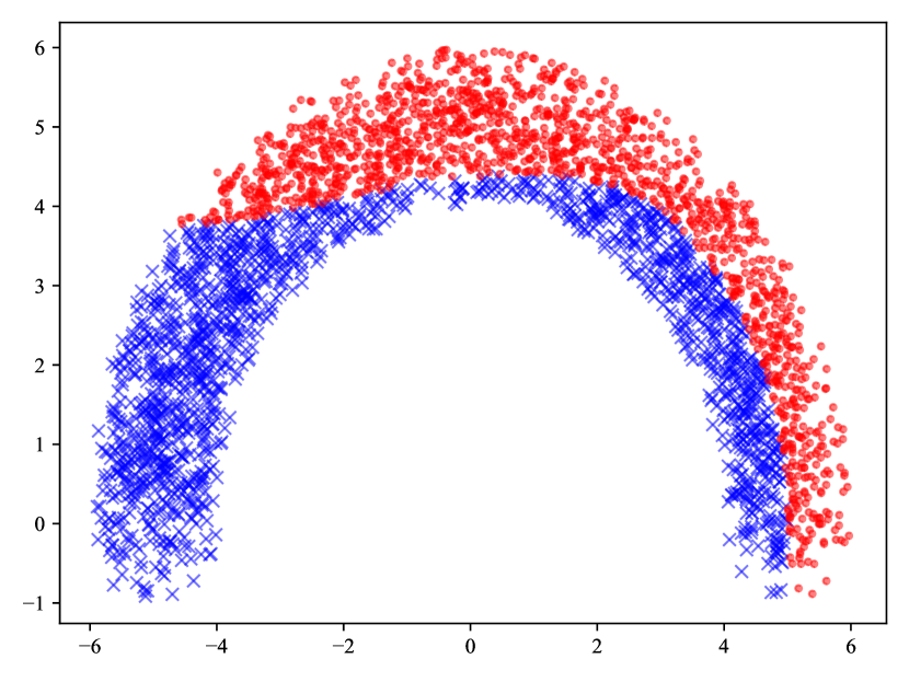
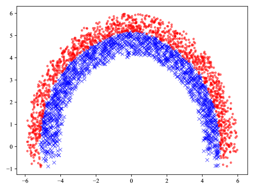
Continuously Indexed Domain Adaptation. We compare DANN+ELS with state-of-the-art continuously indexed domain adaptation methods. Table 5 compares the accuracy of various methods. DANN shows an inferior performance to CIDA. However, with ELS, DANN+ELS boosts the generalization performance by a large margin and beats the SOTA method CIDA (Wang et al., 2020). We also visualize the classification results on Circle Dataset (See Appendix C.1.1 for dataset details). Figure 3 shows that the representative DA method (ADDA) performs poorly when asked to align domains with continuous indices. However, the proposed DANN+ELS can get a near-optimal decision boundary.

Table 5: Rotating MNIST accuracy (%) at the source domain and each target domain. Xsuperscript𝑋X^{\circ} denotes the domain whose images are Rotating by [X,X+45]superscript𝑋superscript𝑋superscript45[X^{\circ},X^{\circ}+45^{\circ}].
Rotating MNIST
Algorithm 0superscript00^{\circ}(Source) 45 90 135 180 225 270 315 Average
ERM (Vapnik, 1999) 99.2 79.7 26.8 31.6 35.1 37.0 28.6 76.2 45.0
ADDA (Tzeng et al., 2017) 97.6 70.7 22.2 32.6 38.2 31.5 20.9 65.8 40.3
DANN (Ganin et al., 2016) 98.4 81.4 38.9 35.4 40.0 43.4 48.8 77.3 52.1
CIDA (Wang et al., 2020) 99.5 80.0 33.2 49.3 50.2 51.7 54.6 81.0 57.1
DANN+ELS 98.4 81.4 55.0 39.9 43.7 45.9 53.7 78.7 62.1
\uparrow 0.0 0.0 16.1 4.5 3.7 2.5 4.9 1.4 10.0
Refer to caption
(a) Domains.
Refer to caption
(b) Ground Truth.
Refer to caption
(c) ADDA.
Refer to caption
(d) DANN+ELS
Figure 3: Results on the Circle dataset with 30 domains. (a) shows domain index by color, (b) shows label index by color, where red dots and blue crosses are positive and negative data sample. Source domains contain the first 6 domains and others are target domains.

Generalization results on other structural datasets and Sequential Datasets. Table 6 shows the generalization results on NLP datasets, and Table 7D.1 show the results on genomics datasets. DANN+ELS bring huge performance improvement on most of the evaluation metrics, e.g., 4.17%percent4.174.17\% test worst-group accuracy on CivilComments, 3.79%percent3.793.79\% test ID accuracy on RxRx1, and 3.13%percent3.133.13\% test accuracy on OGB-MolPCBA. Generalization results on sequential prediction tasks are shown in Table D.1 and Table 18, where DANN works poorly but DANN+ELS brings consistent improvement and beats all baselines on the Spurious-Fourier dataset.

Table 6: Domain generalization performance on neural language datasets. The backbone is DistillBERT-base-uncased and all results are reported over 3 random seed runs.

Amazon-Wilds Algorithm Val Avg Acc Test Avg Acc Val 10% Acc Test 10% Acc Val Worst-group acc Test Worst-group acc ERM (Vapnik, 1999) 72.7 ±plus-or-minus\pm 0.1 71.9 ±plus-or-minus\pm 0.1 55.2 ±plus-or-minus\pm 0.7 53.8 ±plus-or-minus\pm 0.8 20.3 ±plus-or-minus\pm 0.1 4.2 ±plus-or-minus\pm 0.2 Group DRO (Sagawa et al., 2019) 70.7 ±plus-or-minus\pm 0.6 70.0 ±plus-or-minus\pm 0.6 54.7 ±plus-or-minus\pm 0.0 53.3 ±plus-or-minus\pm 0.0 54.2 ±plus-or-minus\pm 0.3 6.3 ±plus-or-minus\pm 0.2 CORAL (Sun & Saenko, 2016) 72.0 ±plus-or-minus\pm 0.3 71.1 ±plus-or-minus\pm 0.3 54.7 ±plus-or-minus\pm 0.0 52.9 ±plus-or-minus\pm 0.8 30.0 ±plus-or-minus\pm 0.2 6.1 ±plus-or-minus\pm 0.1 IRM (Arjovsky et al., 2019) 71.5 ±plus-or-minus\pm 0.3 70.5 ±plus-or-minus\pm 0.3 54.2 ±plus-or-minus\pm 0.8 52.4 ±plus-or-minus\pm 0.8 32.2 ±plus-or-minus\pm 0.8 5.3 ±plus-or-minus\pm 0.2 Reweight 69.1 ±plus-or-minus\pm 0.5 68.6 ±plus-or-minus\pm 0.6 52.1 ±plus-or-minus\pm 0.2 52.0 ±plus-or-minus\pm 0.0 34.9 ±plus-or-minus\pm 1.2 9.1 ±plus-or-minus\pm 0.4 DANN (Ganin et al., 2016) 72.1 ±plus-or-minus\pm 0.2 71.3 ±plus-or-minus\pm 0.1 54.6 ±plus-or-minus\pm 0.0 52.9 ±plus-or-minus\pm 0.6 4.4 ±plus-or-minus\pm 1.3 8.0 ±plus-or-minus\pm 0.0 DANN+ELS 72.3 ±plus-or-minus\pm 0.1 71.5 ±plus-or-minus\pm 0.1 54.7 ±plus-or-minus\pm 0.0 53.8 ± 0.0 4.9 ± 0.6 9.4 ± 0.0 \uparrow 0.2 0.2 0.1 0.9 0.5 1.4

CivilComments-Wilds Algorithm Val Avg Acc Val Worst-Group Acc Test Avg Acc Test Worst-Group Acc Group DRO (Sagawa et al., 2019) 90.4 ±plus-or-minus\pm 0.4 65.0 ±plus-or-minus\pm 3.8 90.2 ±plus-or-minus\pm 0.3 69.1 ±plus-or-minus\pm 1.8 Reweighted 90.0 ±plus-or-minus\pm 0.7 63.7 ±plus-or-minus\pm 2.7 89.8 ±plus-or-minus\pm 0.8 66.6 ±plus-or-minus\pm 1.6 IRM (Arjovsky et al., 2019) 89.0 ±plus-or-minus\pm 0.7 65.9 ±plus-or-minus\pm 2.8 88.8 ±plus-or-minus\pm 0.7 66.3 ±plus-or-minus\pm 2.1 ERM (Vapnik, 1999) 92.3 ±plus-or-minus\pm 0.2 50.5 ±plus-or-minus\pm 1.9 92.2 ±plus-or-minus\pm 0.1 56.0 ±plus-or-minus\pm 3.6 DANN (Ganin et al., 2016) 87.0 ± 0.3 64.0 ± 2.0 87.0 ± 0.3 61.7 ± 2.2 DANN+ELS 88.5 ± 0.4 65.9 ± 1.1 88.4 ± 0.4 66.0 ± 2.2 \uparrow 1.4 1.9 1.4 4.3

Table 7: Domain generalization performance on genomics dataset, RxRx1.

RxRx1-Wilds Algorithm Val Acc Test ID Acc Test Acc Val Worst-Group Acc Test ID Worst-Group Acc Test Worst-Group Acc ERM (Vapnik, 1999) 19.4 ± 0.2 35.9 ± 0.4 29.9 ± 0.4 Group DRO (Sagawa et al., 2019) 15.2 ± 0.1 28.1 ± 0.3 23.0 ± 0.3 IRM (Arjovsky et al., 2019) 5.6 ± 0.4 9.9 ± 1.4 8.2 ± 1.1 0.8 ± 0.2 1.9 ± 0.4 1.5 ± 0.2 DANN (Ganin et al., 2016) 12.7 ± 0.2 22.9 ± 0.1 19.2 ± 0.1 1.0 ± 0.1 4.6 ± 0.4 3.6 ± 0.0 DANN+ELS 14.1 ± 0.1 26.7 ± 0.1 21.2 ± 0.2 1.1 ± 0.1 7.2 ± 0.3 4.2 ± 0.1 \uparrow 1.4 3.8 2 0.1 2.6 0.6

Refer to caption
Refer to caption
Refer to caption
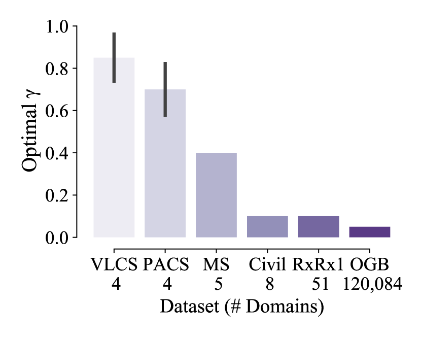
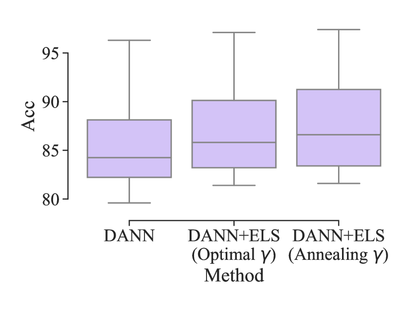
Figure 4: (a) Generalization performance of DANN+ELS compared to DANN with partial correct environment label on the PACS dataset (P𝑃P as target domain). (b) The best γ𝛾\gamma for each dataset. Civil is the CivilComments dataset and OGB is the OGB-MolPCBA dataset. (c) Average generalization accuracy on the PACS dataset with different smoothing policies.

4.2 Interpretation and Analysis

To choose the best γ𝛾\gamma. Figure 4 visualizes the best γ𝛾\gamma values in our experiments. For datasets like PACS and VLCS, where each domain will be set as a target domain respectively and has one best γ𝛾\gamma, we calculate the mean and standard deviation of all these γ𝛾\gamma values. Our main observation is that, as the number of domains increases, the optimal γ𝛾\gamma will also decrease, which is intuitive because more domains mean that the discriminator is more likely to overfit and thus needs a lower γ𝛾\gamma to solve the problem. An interesting thing is that in Figure 4, PACS and VLCS both have 444 domains, but VLCS needs a higher γ𝛾\gamma. Figure 6 shows that images from different domains in PACS are of great visual difference and can be easily discriminated. In contrast, domains in VLCS do not show significant visual differences, and it is hard to discriminate which domain one image belongs to. The discrimination difficulty caused by this inter-domain distinction is another important factor affecting the selection of γ𝛾\gamma.

Annealing γ𝛾\gamma. To achieve better generalization performance and avoid troublesome parametric searches, we propose to gradually decrease γ𝛾\gamma as training progresses, specifically, γ=1.0M1MtT𝛾1.0𝑀1𝑀𝑡𝑇\gamma=1.0-\frac{M-1}{M}\frac{t}{T}, where t,T𝑡𝑇t,T are the current training step and the total training steps. Figure 4 shows that annealing γ𝛾\gamma achieves a comparable or even better generalization performance than fine-grained searched γ𝛾\gamma.

Refer to caption
(a) Classification loss.
Refer to caption
(b) Avg accuracy of source domains.
Refer to caption
(c) Acc on the target domain.
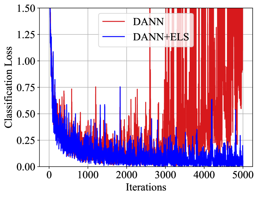
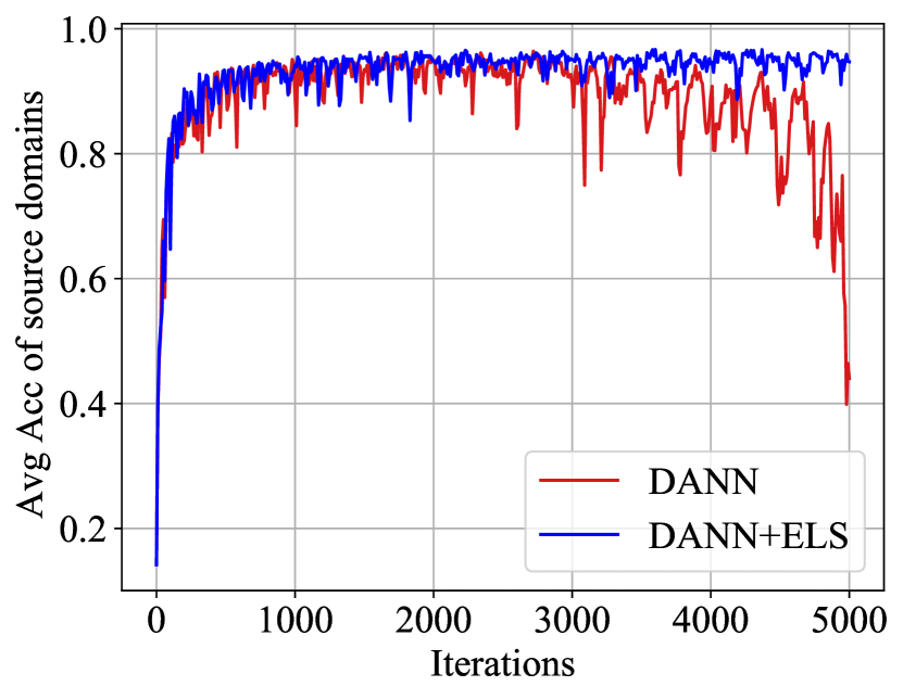
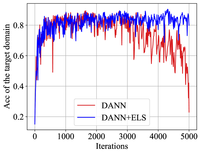
Figure 5: Training statistics on PACS datasets. Alternating GD with nd=5,ne=1formulae-sequencesubscript𝑛𝑑5subscript𝑛𝑒1n_{d}=5,n_{e}=1 is used. All other parameters setting are the same and only on the default hyperparameters and without the fine-grained parametric search.

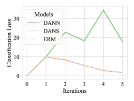
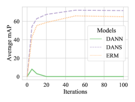
Empirical Verification of our theoretical results. We use the PACS dataset as an example to empirically support our theoretical results, namely verifying the benefits to convergence, training stability, and generalization results. In Figure 5, ’A’ is set as the target domain and other domains as sources. Considering ELS, we can see that in all the experimental results, DANN+ELS with appropriate γ𝛾\gamma attains high training stability, faster and stable convergence, and better performance compared to DANN. In comparison, the training dynamics of native DANN is highly oscillatory, especially in the middle and late stages of training.

5 Related Works

Label Smoothing and Analysis is a technique from the 1980s, and independently re-discovered by (Szegedy et al., 2016). Recently, label smoothing is shown to reduce the vulnerability of neural networks (Warde-Farley & Goodfellow, 2016) and reduce the risk of adversarial examples in GANs (Salimans et al., 2016). Several works seek to theoretically or empirically study the effect of label smoothing. (Chen et al., 2020) focus on studying the minimizer of the training error and finding the optimal smoothing parameter. (Xu et al., 2020) analyzes the convergence behaviors of stochastic gradient descent with label smoothing. However, as far as we know, no study focuses on the effect of label smoothing on the convergence speed and training stability of DAT.

Domain Adversarial Training (Ganin et al., 2016) using a domain discriminator to distinguish the source and target domains and the gradients of the discriminator to the encoder are reversed by the Gradient Reversal layer (GRL), which achieves the goal of learning domain invariant features. (Schoenauer-Sebag et al., 2019; Zhao et al., 2018) extend generalization bounds in DANN (Ganin et al., 2016) to multi-source domains and propose multisource domain adversarial networks. (Acuna et al., 2022) interprets the DAT framework through the lens of game theory and proposes to replace gradient descent with high-order ODE solvers. (Rangwani et al., 2022) finds that enforcing the smoothness of the classifier leads to better generalization on the target domain and presents Smooth Domain Adversarial Training (SDAT). The proposed method is orthogonal to existing DAT methods and yields excellent optimization properties theoretically and empirically.

For space limit, the related works about domain adaptation, domain generalization, and adversarial Training in GANs are in the appendix.

6 Conclusion

In this work, we propose a simple approach, i.e., ELS, to optimize the training process of DAT methods from an environment label design perspective, which is orthogonal to most existing DAT methods. Incorporating ELS into DAT methods is empirically and theoretically shown to be capable of improving robustness to noisy environment labels, converge faster, attain more stable training and better generalization performance. As far as we know, our work takes a first step towards utilizing and understanding label smoothing for environmental labels. Although ELS is designed for DAT methods, reducing the effect of environment label noise and a soft environment partition may benefit all DG/DA methods, which is a promising future direction.

References

  • Acuna et al. (2021) David Acuna, Guojun Zhang, Marc T Law, and Sanja Fidler. f-domain adversarial learning: Theory and algorithms. In International Conference on Machine Learning, pp.  66–75. PMLR, 2021.
  • Acuna et al. (2022) David Acuna, Marc T Law, Guojun Zhang, and Sanja Fidler. Domain adversarial training: A game perspective. ICLR, 2022.
  • Albuquerque et al. (2019) Isabela Albuquerque, João Monteiro, Mohammad Darvishi, Tiago H Falk, and Ioannis Mitliagkas. Generalizing to unseen domains via distribution matching. arXiv preprint arXiv:1911.00804, 2019.
  • Arjovsky & Bottou (2017) Martin Arjovsky and Léon Bottou. Towards principled methods for training generative adversarial networks. arXiv preprint arXiv:1701.04862, 2017.
  • Arjovsky et al. (2017) Martin Arjovsky, Soumith Chintala, and Léon Bottou. Wasserstein generative adversarial networks. In International conference on machine learning, pp. 214–223. PMLR, 2017.
  • Arjovsky et al. (2019) Martin Arjovsky, Léon Bottou, Ishaan Gulrajani, and David Lopez-Paz. Invariant risk minimization. arXiv preprint arXiv:1907.02893, 2019.
  • Arora et al. (2017) Sanjeev Arora, Rong Ge, Yingyu Liang, Tengyu Ma, and Yi Zhang. Generalization and equilibrium in generative adversarial nets (gans). In International Conference on Machine Learning, pp. 224–232. PMLR, 2017.
  • Ben-David et al. (2006) Shai Ben-David, John Blitzer, Koby Crammer, and Fernando Pereira. Analysis of representations for domain adaptation. In NIPS, 2006.
  • Ben-David et al. (2010) Shai Ben-David, John Blitzer, Koby Crammer, Alex Kulesza, Fernando Pereira, and Jennifer Wortman Vaughan. A theory of learning from different domains. Machine learning, 2010.
  • Bertsekas (1999) Dimitri P Bertsekas. Nonlinear programming. In thena scientific Belmont, 1999.
  • Blanchard et al. (2021) Gilles Blanchard, Aniket Anand Deshmukh, Ürün Dogan, Gyemin Lee, and Clayton Scott. Domain generalization by marginal transfer learning. J. Mach. Learn. Res., 2021.
  • Brock et al. (2019) Andrew Brock, Jeff Donahue, and Karen Simonyan. Large scale gan training for high fidelity natural image synthesis. International Conference on Learning Representations (ICLR), 2019.
  • Chen et al. (2020) Blair Chen, Liu Ziyin, Zihao Wang, and Paul Pu Liang. An investigation of how label smoothing affects generalization. arXiv preprint arXiv:2010.12648, 2020.
  • Chen et al. (2021) Peixian Chen, Pingyang Dai, Jianzhuang Liu, Feng Zheng, Qi Tian, and Rongrong Ji. Dual distribution alignment network for generalizable person re-identification. AAAI Conference on Artificial Intelligence, 2021.
  • Chen et al. (2018) Xu Chen, Jiang Wang, and Hao Ge. Training generative adversarial networks via primal-dual subgradient methods: a lagrangian perspective on gan. arXiv preprint arXiv:1802.01765, 2018.
  • Choi et al. (2021) Seokeon Choi, Taekyung Kim, Minki Jeong, Hyoungseob Park, and Changick Kim. Meta batch-instance normalization for generalizable person re-identification. In Computer Vision and Pattern Recognition (CVPR), 2021.
  • Creager et al. (2021) Elliot Creager, Jörn-Henrik Jacobsen, and Richard Zemel. Environment inference for invariant learning. In ICML, 2021.
  • Deng et al. (2009) Jia Deng, Wei Dong, Richard Socher, Li-Jia Li, Kai Li, and Li Fei-Fei. Imagenet: A large-scale hierarchical image database. In Computer Vision and Pattern Recognition (CVPR), 2009.
  • Farnia & Ozdaglar (2020) Farzan Farnia and Asuman Ozdaglar. Do GANs always have Nash equilibria? In Hal Daumé III and Aarti Singh (eds.), Proceedings of the 37th International Conference on Machine Learning, volume 119 of Proceedings of Machine Learning Research, pp.  3029–3039. PMLR, 13–18 Jul 2020. URL https://proceedings.mlr.press/v119/farnia20a.html.
  • Gagnon-Audet et al. (2022) Jean-Christophe Gagnon-Audet, Kartik Ahuja, Mohammad-Javad Darvishi-Bayazi, Guillaume Dumas, and Irina Rish. Woods: Benchmarks for out-of-distribution generalization in time series tasks. arXiv preprint arXiv:2203.09978, 2022.
  • Gan et al. (2017) Zhe Gan, Liqun Chen, Weiyao Wang, Yuchen Pu, Yizhe Zhang, Hao Liu, Chunyuan Li, and Lawrence Carin. Triangle generative adversarial networks. Advances in neural information processing systems, 30, 2017.
  • Ganin et al. (2016) Yaroslav Ganin, Evgeniya Ustinova, Hana Ajakan, Pascal Germain, Hugo Larochelle, François Laviolette, Mario Marchand, and Victor Lempitsky. Domain-adversarial training of neural networks. The journal of machine learning research, 2016.
  • Geirhos et al. (2020) Robert Geirhos, Jörn-Henrik Jacobsen, Claudio Michaelis, Richard Zemel, Wieland Brendel, Matthias Bethge, and Felix A. Wichmann. Shortcut learning in deep neural networks. Nature Machine Intelligence, 2020.
  • Ghifary et al. (2015) Muhammad Ghifary, W Bastiaan Kleijn, Mengjie Zhang, and David Balduzzi. Domain generalization for object recognition with multi-task autoencoders. In ICCV, 2015.
  • Gidel et al. (2018) Gauthier Gidel, Hugo Berard, Gaëtan Vignoud, Pascal Vincent, and Simon Lacoste-Julien. A variational inequality perspective on generative adversarial networks. arXiv preprint arXiv:1802.10551, 2018.
  • Goodfellow (2016) Ian Goodfellow. Nips 2016 tutorial: Generative adversarial networks. arXiv preprint arXiv:1701.00160, 2016.
  • Goodfellow et al. (2014) Ian Goodfellow, Jean Pouget-Abadie, Mehdi Mirza, Bing Xu, David Warde-Farley, Sherjil Ozair, Aaron Courville, and Yoshua Bengio. Generative adversarial nets. Advances in neural information processing systems, 27, 2014.
  • Gray et al. (2007) D. Gray, S. Brennan, and H. Tao. Evaluating Appearance Models for Recognition, Reacquisition, and Tracking. Proc. IEEE International Workshop on Performance Evaluation for Tracking and Surveillance (PETS), 2007.
  • Gulrajani & Lopez-Paz (2021) Ishaan Gulrajani and David Lopez-Paz. In search of lost domain generalization. In ICLR, 2021.
  • He et al. (2016) Kaiming He, Xiangyu Zhang, Shaoqing Ren, and Jian Sun. Deep residual learning for image recognition. In Proceedings of the IEEE conference on computer vision and pattern recognition, pp.  770–778, 2016.
  • Hirzer et al. (2011) Martin Hirzer, Csaba Beleznai, Peter M Roth, and Horst Bischof. Person re-identification by descriptive and discriminative classification. In Scandinavian Conference on Image Analysis, 2011.
  • Jaderberg et al. (2015) Max Jaderberg, Karen Simonyan, Andrew Zisserman, et al. Spatial transformer networks. Advances in neural information processing systems, 28, 2015.
  • Jenni & Favaro (2019) Simon Jenni and Paolo Favaro. On stabilizing generative adversarial training with noise. In Proceedings of the IEEE/CVF Conference on Computer Vision and Pattern Recognition, pp.  12145–12153, 2019.
  • Jia et al. (2019) Jieru Jia, Qiuqi Ruan, and Timothy M Hospedales. Frustratingly easy person re-identification: Generalizing person re-id in practice. arXiv preprint arXiv:1905.03422, 2019.
  • Jin et al. (2020) Ying Jin, Ximei Wang, Mingsheng Long, and Jianmin Wang. Less confusion more transferable: Minimum class confusion for versatile domain adaptation. In ECCV, 2020.
  • Khalil. (1996) Hassan K Khalil. Non-linear Systems. Prentice-Hall, New Jersey,, 1996.
  • Kim et al. (2019) Youngdong Kim, Junho Yim, Juseung Yun, and Junmo Kim. Nlnl: Negative learning for noisy labels. In Proceedings of the IEEE/CVF International Conference on Computer Vision, pp.  101–110, 2019.
  • Koh et al. (2021) Pang Wei Koh, Shiori Sagawa, Sang Michael Xie, Marvin Zhang, Akshay Balsubramani, Weihua Hu, Michihiro Yasunaga, Richard Lanas Phillips, Irena Gao, Tony Lee, et al. Wilds: A benchmark of in-the-wild distribution shifts. In ICML, 2021.
  • Krueger et al. (2021) David Krueger, Ethan Caballero, Joern-Henrik Jacobsen, Amy Zhang, Jonathan Binas, Dinghuai Zhang, Remi Le Priol, and Aaron Courville. Out-of-distribution generalization via risk extrapolation (rex). In ICML, 2021.
  • Li et al. (2017a) Chun-Liang Li, Wei-Cheng Chang, Yu Cheng, Yiming Yang, and Barnabás Póczos. Mmd gan: Towards deeper understanding of moment matching network. Advances in neural information processing systems, 30, 2017a.
  • Li et al. (2017b) Da Li, Yongxin Yang, Yi-Zhe Song, and Timothy M Hospedales. Deeper, broader and artier domain generalization. In ICCV, 2017b.
  • Li et al. (2018a) Da Li, Yongxin Yang, Yi-Zhe Song, and Timothy Hospedales. Learning to generalize: Meta-learning for domain generalization. In AAAI, 2018a.
  • Li & Wang (2013) Wei Li and Xiaogang Wang. Locally aligned feature transforms across views. In Computer Vision and Pattern Recognition (CVPR), June 2013.
  • Li et al. (2014) Wei Li, Rui Zhao, Tong Xiao, and Xiaogang Wang. Deepreid: Deep filter pairing neural network for person re-identification. In Computer Vision and Pattern Recognition (CVPR), June 2014.
  • Li et al. (2018b) Ya Li, Xinmei Tian, Mingming Gong, Yajing Liu, Tongliang Liu, Kun Zhang, and Dacheng Tao. Deep domain generalization via conditional invariant adversarial networks. In ECCV, 2018b.
  • Liu et al. (2012) Chunxiao Liu, Shaogang Gong, Chen Change Loy, and Xinggang Lin. Person re-identification: What features are important? In European Conference on Computer Vision (ECCV). Springer, 2012.
  • Long et al. (2018) Mingsheng Long, Zhangjie Cao, Jianmin Wang, and Michael I Jordan. Conditional adversarial domain adaptation. Advances in neural information processing systems, 31, 2018.
  • Mescheder et al. (2017) Lars Mescheder, Sebastian Nowozin, and Andreas Geiger. The numerics of gans. Advances in neural information processing systems, 30, 2017.
  • Mescheder et al. (2018) Lars Mescheder, Andreas Geiger, and Sebastian Nowozin. Which training methods for gans do actually converge? In ICML, 2018.
  • Muandet et al. (2013) K. Muandet, D. Balduzzi, and B. Schölkopf. Domain generalization via invariant feature representation. In ICML, 2013.
  • Nagarajan & Kolter (2017) Vaishnavh Nagarajan and J Zico Kolter. Gradient descent gan optimization is locally stable. Advances in neural information processing systems, 30, 2017.
  • Nguyen et al. (2017) Tu Nguyen, Trung Le, Hung Vu, and Dinh Phung. Dual discriminator generative adversarial nets. Advances in neural information processing systems, 30, 2017.
  • Nie & Patel (2020) Weili Nie and Ankit B Patel. Towards a better understanding and regularization of gan training dynamics. In Uncertainty in Artificial Intelligence, pp.  281–291. PMLR, 2020.
  • Nowozin et al. (2016) Sebastian Nowozin, Botond Cseke, and Ryota Tomioka. f-gan: Training generative neural samplers using variational divergence minimization. Advances in neural information processing systems, 29, 2016.
  • Pezeshki et al. (2021) Mohammad Pezeshki, Oumar Kaba, Yoshua Bengio, Aaron C Courville, Doina Precup, and Guillaume Lajoie. Gradient starvation: A learning proclivity in neural networks. Advances in Neural Information Processing Systems, 34, 2021.
  • Pu et al. (2018) Yunchen Pu, Shuyang Dai, Zhe Gan, Weiyao Wang, Guoyin Wang, Yizhe Zhang, Ricardo Henao, and Lawrence Carin Duke. Jointgan: Multi-domain joint distribution learning with generative adversarial nets. In International Conference on Machine Learning, pp. 4151–4160. PMLR, 2018.
  • Rame et al. (2021) Alexandre Rame, Corentin Dancette, and Matthieu Cord. Fishr: Invariant gradient variances for out-of-distribution generalization. arXiv preprint arXiv:2109.02934, 2021.
  • Rangwani et al. (2022) Harsh Rangwani, Sumukh K Aithal, Mayank Mishra, Arihant Jain, and R Venkatesh Babu. A closer look at smoothness in domain adversarial training. ICML, 2022.
  • Roth et al. (2017) Kevin Roth, Aurélien Lucchi, Sebastian Nowozin, and Thomas Hofmann. Stabilizing training of generative adversarial networks through regularization. In NIPS, 2017.
  • Russakovsky et al. (2015) Olga Russakovsky, Jia Deng, Hao Su, Jonathan Krause, Sanjeev Satheesh, Sean Ma, Zhiheng Huang, Andrej Karpathy, Aditya Khosla, Michael Bernstein, et al. Imagenet large scale visual recognition challenge. IJCV, 2015.
  • Saenko et al. (2010) Kate Saenko, Brian Kulis, Mario Fritz, and Trevor Darrell. Adapting visual category models to new domains. In European conference on computer vision, pp.  213–226. Springer, 2010.
  • Sagawa et al. (2019) Shiori Sagawa, Pang Wei Koh, Tatsunori B Hashimoto, and Percy Liang. Distributionally robust neural networks for group shifts: On the importance of regularization for worst-case generalization. arXiv preprint arXiv:1911.08731, 2019.
  • Salimans et al. (2016) Tim Salimans, Ian Goodfellow, Wojciech Zaremba, Vicki Cheung, Alec Radford, and Xi Chen. Improved techniques for training gans. Advances in neural information processing systems, 29, 2016.
  • Sandler et al. (2018) Mark Sandler, Andrew Howard, Menglong Zhu, Andrey Zhmoginov, and Liang-Chieh Chen. Mobilenetv2: Inverted residuals and linear bottlenecks. In Computer Vision and Pattern Recognition (CVPR), 2018.
  • Schirrmeister et al. (2017) Robin Tibor Schirrmeister, Jost Tobias Springenberg, Lukas Dominique Josef Fiederer, Martin Glasstetter, Katharina Eggensperger, Michael Tangermann, Frank Hutter, Wolfram Burgard, and Tonio Ball. Deep learning with convolutional neural networks for eeg decoding and visualization. Human brain mapping, 38(11):5391–5420, 2017.
  • Schoenauer-Sebag et al. (2019) Alice Schoenauer-Sebag, Louise Heinrich, Marc Schoenauer, Michele Sebag, Lani F Wu, and Steve J Altschuler. Multi-domain adversarial learning. arXiv preprint arXiv:1903.09239, 2019.
  • Schäfer et al. (2019) Florian Schäfer, Hongkai Zheng, and Anima Anandkumar. Implicit competitive regularization in gans, 2019.
  • Sønderby et al. (2016) Casper Kaae Sønderby, Jose Caballero, Lucas Theis, Wenzhe Shi, and Ferenc Huszár. Amortised map inference for image super-resolution. arXiv preprint arXiv:1610.04490, 2016.
  • Song et al. (2019) Jifei Song, Yongxin Yang, Yi-Zhe Song, Tao Xiang, and Timothy M. Hospedales. Generalizable person re-identification by domain-invariant mapping network. In Computer Vision and Pattern Recognition (CVPR), June 2019.
  • Sun & Saenko (2016) Baochen Sun and Kate Saenko. Deep coral: Correlation alignment for deep domain adaptation. In European conference on computer vision, pp.  443–450. Springer, 2016.
  • Szegedy et al. (2016) Christian Szegedy, Vincent Vanhoucke, Sergey Ioffe, Jon Shlens, and Zbigniew Wojna. Rethinking the inception architecture for computer vision. In Proceedings of the IEEE conference on computer vision and pattern recognition, pp.  2818–2826, 2016.
  • Tang et al. (2020) Hui Tang, Ke Chen, and Kui Jia. Unsupervised domain adaptation via structurally regularized deep clustering. In Proceedings of the IEEE/CVF conference on computer vision and pattern recognition, pp.  8725–8735, 2020.
  • Tao et al. (2018) Chenyang Tao, Liqun Chen, Ricardo Henao, Jianfeng Feng, and Lawrence Carin Duke. Chi-square generative adversarial network. In International conference on machine learning, pp. 4887–4896. PMLR, 2018.
  • Thanh-Tung et al. (2019) Hoang Thanh-Tung, Truyen Tran, and Svetha Venkatesh. Improving generalization and stability of generative adversarial networks. arXiv preprint arXiv:1902.03984, 2019.
  • Torralba & Efros (2011) Antonio Torralba and Alexei A Efros. Unbiased look at dataset bias. In CVPR, 2011.
  • Trung Le et al. (2019) Quan Hoang Trung Le, Hung Vu, Tu Dinh Nguyen, Hung Bui, and Dinh Phung. Learning generative adversarial networks from multiple data sources. In Proceedings of the 28th International Joint Conference on Artificial Intelligence, 2019.
  • Tzeng et al. (2017) Eric Tzeng, Judy Hoffman, Kate Saenko, and Trevor Darrell. Adversarial discriminative domain adaptation. In Proceedings of the IEEE conference on computer vision and pattern recognition, pp.  7167–7176, 2017.
  • Vapnik (1999) Vladimir Vapnik. The nature of statistical learning theory. Springer science & business media, 1999.
  • Venkateswara et al. (2017) Hemanth Venkateswara, Jose Eusebio, Shayok Chakraborty, and Sethuraman Panchanathan. Deep hashing network for unsupervised domain adaptation. In Proceedings of the IEEE conference on computer vision and pattern recognition, pp.  5018–5027, 2017.
  • Wang et al. (2020) Hao Wang, Hao He, and Dina Katabi. Continuously indexed domain adaptation. ICML, 2020.
  • (81) Jindong Wang and Wenxin Hou. Deepda: Deep domain adaptation toolkit. https://github.com/jindongwang/transferlearning/tree/master/code/DeepDA.
  • Warde-Farley & Goodfellow (2016) David Warde-Farley and Ian Goodfellow. 11 adversarial perturbations of deep neural networks. Perturbations, Optimization, and Statistics, 311:5, 2016.
  • Wei et al. (2022) Jiaheng Wei, Hangyu Liu, Tongliang Liu, Gang Niu, Masashi Sugiyama, and Yang Liu. To smooth or not? when label smoothing meets noisy labels. ICML, 2022.
  • Wei-Shi et al. (2009) Zheng Wei-Shi, Gong Shaogang, and Xiang Tao. Associating groups of people. In British Machine Vision Conference (BMVC), 2009.
  • Wolf et al. (2019) Thomas Wolf, Lysandre Debut, Victor Sanh, Julien Chaumond, Clement Delangue, Anthony Moi, Pierric Cistac, Tim Rault, Rémi Louf, Morgan Funtowicz, et al. Huggingface’s transformers: State-of-the-art natural language processing. arXiv preprint arXiv:1910.03771, 2019.
  • Xiao et al. (2016) Tong Xiao, Shuang Li, Bochao Wang, Liang Lin, and Xiaogang Wang. End-to-end deep learning for person search. arXiv preprint arXiv:1604.01850, 2(2), 2016.
  • Xu et al. (2018) Keyulu Xu, Weihua Hu, Jure Leskovec, and Stefanie Jegelka. How powerful are graph neural networks? arXiv preprint arXiv:1810.00826, 2018.
  • Xu et al. (2020) Yi Xu, Yuanhong Xu, Qi Qian, Hao Li, and Rong Jin. Towards understanding label smoothing. arXiv preprint arXiv:2006.11653, 2020.
  • Yadav et al. (2017) Abhay Yadav, Sohil Shah, Zheng Xu, David Jacobs, and Tom Goldstein. Stabilizing adversarial nets with prediction methods. arXiv preprint arXiv:1705.07364, 2017.
  • Yang et al. (2021) Jinyu Yang, Jingjing Liu, Ning Xu, and Junzhou Huang. Tvt: Transferable vision transformer for unsupervised domain adaptation. arXiv preprint arXiv:2108.05988, 2021.
  • Zhang et al. (2021a) Hanlin Zhang, Yi-Fan Zhang, Weiyang Liu, Adrian Weller, Bernhard Schölkopf, and Eric P Xing. Towards principled disentanglement for domain generalization. arXiv preprint arXiv:2111.13839, 2021a.
  • Zhang et al. (2021b) Marvin Zhang, Henrik Marklund, Nikita Dhawan, Abhishek Gupta, Sergey Levine, and Chelsea Finn. Adaptive risk minimization: Learning to adapt to domain shift. NeurIPS, 2021b.
  • Zhang et al. (2021c) Yi-Fan Zhang, Zhang Zhang, Da Li, Zhen Jia, Liang Wang, and Tieniu Tan. Learning domain invariant representations for generalizable person re-identification. arXiv preprint arXiv:2103.15890, 2021c.
  • Zhang et al. (2022) YiFan Zhang, Feng Li, Zhang Zhang, Liang Wang, Dacheng Tao, and Tieniu Tan. Generalizable person re-identification without demographics, 2022. URL https://openreview.net/forum?id=VNdFPD5wqjh.
  • Zhang et al. (2019) Yuchen Zhang, Tianle Liu, Mingsheng Long, and Michael Jordan. Bridging theory and algorithm for domain adaptation. In International Conference on Machine Learning, pp. 7404–7413. PMLR, 2019.
  • Zhao et al. (2018) Han Zhao, Shanghang Zhang, Guanhang Wu, José MF Moura, Joao P Costeira, and Geoffrey J Gordon. Adversarial multiple source domain adaptation. In NeurIPS, 2018.
  • Zheng et al. (2015) Liang Zheng, Liyue Shen, Lu Tian, Shengjin Wang, Jingdong Wang, and Qi Tian. Scalable person re-identification: A benchmark. In International Conference on Computer Vision (ICCV), December 2015.
  • Zheng et al. (2017) Zhedong Zheng, Liang Zheng, and Yi Yang. Unlabeled samples generated by gan improve the person re-identification baseline in vitro. In International Conference on Computer Vision (ICCV), Oct 2017.

Appendix

Appendix A Proofs of Theoretical Statements

Table 8: Notations.
Symbol Description
𝒟S,𝒟T,𝒟isubscript𝒟𝑆subscript𝒟𝑇subscript𝒟𝑖\mathcal{D}_{S},\mathcal{D}_{T},\mathcal{D}_{i} Distributions for source domain, target domain, and domain i𝑖i.
𝒟^S,𝒟^T,𝒟^isubscript^𝒟𝑆subscript^𝒟𝑇subscript^𝒟𝑖\hat{\mathcal{D}}_{S},\hat{\mathcal{D}}_{T},\hat{\mathcal{D}}_{i} Empirical distributions for source domain, target domain, and domain i𝑖i.
ps,pt,pisubscript𝑝𝑠subscript𝑝𝑡subscript𝑝𝑖p_{s},p_{t},p_{i} Density functions for source domain, target domain, and domain i𝑖i.
𝐱s,𝐱t,𝐱isubscript𝐱𝑠subscript𝐱𝑡subscript𝐱𝑖\mathbf{x}_{s},\mathbf{x}_{t},\mathbf{x}_{i} Data samples from source domain, target domain, and domain i𝑖i.
𝒟Sz,𝒟Tz,𝒟izsubscriptsuperscript𝒟𝑧𝑆subscriptsuperscript𝒟𝑧𝑇subscriptsuperscript𝒟𝑧𝑖\mathcal{D}^{z}_{S},\mathcal{D}^{z}_{T},\mathcal{D}^{z}_{i}
Feature distributions of 𝒟S,𝒟T,𝒟isubscript𝒟𝑆subscript𝒟𝑇subscript𝒟𝑖\mathcal{D}_{S},\mathcal{D}_{T},\mathcal{D}_{i} respectively,
which is also termed g𝒟S,g𝒟T,g𝒟i𝑔subscript𝒟𝑆𝑔subscript𝒟𝑇𝑔subscript𝒟𝑖g\circ\mathcal{D}_{S},g\circ\mathcal{D}_{T},g\circ\mathcal{D}_{i}.
psz,ptz,pizsubscriptsuperscript𝑝𝑧𝑠subscriptsuperscript𝑝𝑧𝑡subscriptsuperscript𝑝𝑧𝑖p^{z}_{s},p^{z}_{t},p^{z}_{i} Density functions for 𝒟Sz,𝒟Tz,𝒟izsubscriptsuperscript𝒟𝑧𝑆subscriptsuperscript𝒟𝑧𝑇subscriptsuperscript𝒟𝑧𝑖\mathcal{D}^{z}_{S},\mathcal{D}^{z}_{T},\mathcal{D}^{z}_{i} respectively.
𝐳s,𝐳t,𝐳isubscript𝐳𝑠subscript𝐳𝑡subscript𝐳𝑖\mathbf{z}_{s},\mathbf{z}_{t},\mathbf{z}_{i} Data samples from 𝒟Sz,𝒟Tz,𝒟izsubscriptsuperscript𝒟𝑧𝑆subscriptsuperscript𝒟𝑧𝑇subscriptsuperscript𝒟𝑧𝑖\mathcal{D}^{z}_{S},\mathcal{D}^{z}_{T},\mathcal{D}^{z}_{i}.
,^,𝒢^𝒢\mathcal{H},\hat{\mathcal{H}},\mathcal{G} Support sets for hypothesis, discriminator, and feature encoder.
h,h^,h^,g^superscript^𝑔h,\hat{h},\hat{h}^{*},g Hypothesis, discriminator, the optimal discriminator, and feature encoder.
M,ni𝑀subscript𝑛𝑖M,n_{i} Number of training distributions, number of data samples in 𝒟isubscript𝒟𝑖\mathcal{D}_{i}.
γ𝛾\gamma Hyper-parameter for the environment label smoothing.
d,d^subscript𝑑subscript^𝑑d_{\mathcal{H}},\hat{d}_{\mathcal{H}} \mathcal{H}-divergence and Empirical \mathcal{H}-divergence.

The commonly used notations and their corresponding descriptions are concluded in Table 8.

A.1 Connect Environment Label Smoothing to JS Divergence Minimization

To complete the proofs, we begin by introducing some necessary definitions and assumptions.

Definition 1.

(\mathcal{H}-divergence (Ben-David et al., 2006)). Given two domain distributions 𝒟S,𝒟Tsubscript𝒟𝑆subscript𝒟𝑇\mathcal{D}_{S},\mathcal{D}_{T} over X𝑋X, and a hypothesis class \mathcal{H}, the \mathcal{H}-divergence between 𝒟S,𝒟Tsubscript𝒟𝑆subscript𝒟𝑇\mathcal{D}_{S},\mathcal{D}_{T} is

d(𝒟S,𝒟T)=2suph𝔼𝐱𝒟S[h(𝐱)=1]𝔼𝐱𝒟T[h(𝐱)=1]subscript𝑑subscript𝒟𝑆subscript𝒟𝑇2subscriptsupremumdelimited-∣∣subscript𝔼similar-to𝐱subscript𝒟𝑆delimited-[]𝐱1subscript𝔼similar-to𝐱subscript𝒟𝑇delimited-[]𝐱1d_{\mathcal{H}}(\mathcal{D}_{S},\mathcal{D}_{T})=2\sup_{h\in\mathcal{H}}\left\mid\mathbb{E}_{\mathbf{x}\sim\mathcal{D}_{S}}[h(\mathbf{x})=1]-\mathbb{E}_{\mathbf{x}\sim\mathcal{D}_{T}}[h(\mathbf{x})=1]\right\mid (5)
Definition 2.

(Empirical \mathcal{H}-divergence (Ben-David et al., 2006).) For an symmetric hypothesis class \mathcal{H}, one can compute the empirical \mathcal{H}-divergence between two empirical distributions 𝒟^Ssubscript^𝒟𝑆\hat{\mathcal{D}}_{S} and 𝒟^Tsubscript^𝒟𝑇\hat{\mathcal{D}}_{T} by computing

d^(𝒟^S,𝒟^T)=2(1minh[1mi=1mI[h(𝐱i)=0]+1ni=1nI[h(𝐱i)=1]]),subscript^𝑑subscript^𝒟𝑆subscript^𝒟𝑇21subscript1𝑚superscriptsubscript𝑖1𝑚𝐼delimited-[]subscript𝐱𝑖01𝑛superscriptsubscript𝑖1𝑛𝐼delimited-[]subscript𝐱𝑖1\hat{d}_{\mathcal{H}}(\hat{\mathcal{D}}_{S},\hat{\mathcal{D}}_{T})=2\left(1-\min_{h\in\mathcal{H}}\left[\frac{1}{m}\sum_{i=1}^{m}I[h(\mathbf{x}_{i})=0]+\frac{1}{n}\sum_{i=1}^{n}I[h(\mathbf{x}_{i})=1]\right]\right), (6)

where m,n𝑚𝑛m,n is the number of data samples of 𝒟^Ssubscript^𝒟𝑆\hat{\mathcal{D}}_{S} and 𝒟^Tsubscript^𝒟𝑇\hat{\mathcal{D}}_{T} respectively and I[a]𝐼delimited-[]𝑎I[a] is the indicator function which is 1 if predicate a𝑎a is true, and 0 otherwise.

Vanilla DANN estimating the “min” part of Equ. (6) by a domain discriminator, that models the probability that a given input is from the source domain or the target domain. Specially, let the hypothesis hh be the composition of h=h^g^𝑔h=\hat{h}\circ g, where h^^^^\hat{h}\in\hat{\mathcal{H}} is a additional hypothesis and g𝒢𝑔𝒢g\in\mathcal{G} pushes forward the data samples to a representation space 𝒵𝒵\mathcal{Z}. DANN (Ben-David et al., 2006) seeks to approximate the \mathcal{H}-divergence of Equ. (6) by

maxh^^dh^,g(𝒟S,𝒟T)=maxh^^𝔼𝐱s𝒟Slogh^g(𝐱s)+𝔼𝐱t𝒟Tlog(1h^g(𝐱t)),subscript^^subscript𝑑^𝑔subscript𝒟𝑆subscript𝒟𝑇subscript^^subscript𝔼similar-tosubscript𝐱𝑠subscript𝒟𝑆^𝑔subscript𝐱𝑠subscript𝔼similar-tosubscript𝐱𝑡subscript𝒟𝑇1^𝑔subscript𝐱𝑡\max_{\hat{h}\in\hat{\mathcal{H}}}d_{\hat{h},g}(\mathcal{D}_{S},\mathcal{D}_{T})=\max_{\hat{h}\in\hat{\mathcal{H}}}\mathbb{E}_{\mathbf{x}_{s}\sim\mathcal{D}_{S}}\log\hat{h}\circ g(\mathbf{x}_{s})+\mathbb{E}_{\mathbf{x}_{t}\sim\mathcal{D}_{T}}\log\left(1-\hat{h}\circ g(\mathbf{x}_{t})\right), (7)

where the sigmoid activate function is ignored for simplicity, h^g(𝐱)^𝑔𝐱\hat{h}\circ g(\mathbf{x}) is the prediction probability that 𝐱𝐱\mathbf{x} is belonged to 𝒟Ssubscript𝒟𝑆\mathcal{D}_{S} and 1h^g(𝐱)1^𝑔𝐱1-\hat{h}\circ g(\mathbf{x}) is the prediction probability that 𝐱𝐱\mathbf{x} is belonged to 𝒟Tsubscript𝒟𝑇\mathcal{D}_{T}. Applying environment label smoothing, the target can be reformulated to

maxh^^dh^,g,γ(𝒟S,𝒟T)=maxh^^𝔼𝐱s𝒟Ssubscript^^subscript𝑑^𝑔𝛾subscript𝒟𝑆subscript𝒟𝑇subscript^^subscript𝔼similar-tosubscript𝐱𝑠subscript𝒟𝑆\displaystyle\max_{\hat{h}\in\hat{\mathcal{H}}}d_{\hat{h},g,\gamma}(\mathcal{D}_{S},\mathcal{D}_{T})=\max_{\hat{h}\in\hat{\mathcal{H}}}\mathbb{E}_{\mathbf{x}_{s}\sim\mathcal{D}_{S}} [γlogh^g(𝐱s)+(1γ)log(1h^g(𝐱s))]+limit-fromdelimited-[]𝛾^𝑔subscript𝐱𝑠1𝛾1^𝑔subscript𝐱𝑠\displaystyle\left[\gamma\log\hat{h}\circ g(\mathbf{x}_{s})+(1-\gamma)\log\left(1-\hat{h}\circ g(\mathbf{x}_{s})\right)\right]+ (8)
𝔼𝐱t𝒟T[(1γ)logh^g(𝐱t)+γlog(1h^g(𝐱t))]subscript𝔼similar-tosubscript𝐱𝑡subscript𝒟𝑇delimited-[]1𝛾^𝑔subscript𝐱𝑡𝛾1^𝑔subscript𝐱𝑡\displaystyle\mathbb{E}_{\mathbf{x}_{t}\sim\mathcal{D}_{T}}\left[(1-\gamma)\log\hat{h}\circ g(\mathbf{x}_{t})+\gamma\log\left(1-\hat{h}\circ g(\mathbf{x}_{t})\right)\right]

When γ{0,1}𝛾01\gamma\in\{0,1\}, Equ. (8) is equal to Equ. (7) and no environment label smoothing is applied. Then we prove the proposition 1

Proposition 1. Suppose h^^\hat{h} the optimal domain classifier with no constraint and mixed distributions {𝒟S=γ𝒟S+(1γ)𝒟T𝒟T=γ𝒟T+(1γ)𝒟Scasessubscript𝒟superscript𝑆𝛾subscript𝒟𝑆1𝛾subscript𝒟𝑇subscript𝒟superscript𝑇𝛾subscript𝒟𝑇1𝛾subscript𝒟𝑆\left\{\begin{array}[]{c}\mathcal{D}_{S^{\prime}}=\gamma\mathcal{D}_{S}+(1-\gamma)\mathcal{D}_{T}\\ \mathcal{D}_{T^{\prime}}=\gamma\mathcal{D}_{T}+(1-\gamma)\mathcal{D}_{S}\\ \end{array}\right. with hyper-parameter γ𝛾\gamma, then maxh^^dh^,g,γ(𝒟S,𝒟T)=2DJS(𝒟S||𝒟T)2log2\max_{\hat{h}\in\hat{\mathcal{H}}}d_{\hat{h},g,\gamma}(\mathcal{D}_{S},\mathcal{D}_{T})=2D_{JS}(\mathcal{D}_{S^{\prime}}||\mathcal{D}_{T^{\prime}})-2\log 2, where DJSsubscript𝐷𝐽𝑆D_{JS} is the Jensen-Shanon (JS) divergence.

Proof.

Denote the injected source/target density as psz:=gps,ptz:=gptformulae-sequenceassignsuperscriptsubscript𝑝𝑠𝑧𝑔subscript𝑝𝑠assignsuperscriptsubscript𝑝𝑡𝑧𝑔subscript𝑝𝑡p_{s}^{z}:=g\circ p_{s},p_{t}^{z}:=g\circ p_{t}, where ps,ptsubscript𝑝𝑠subscript𝑝𝑡p_{s},p_{t} is the density of 𝒟S,𝒟Tsubscript𝒟𝑆subscript𝒟𝑇\mathcal{D}_{S},\mathcal{D}_{T} respectively. We can rewrite Equ. (8) as:

dh^,g,γ(𝒟S,𝒟T)=𝒵psz(𝐳)log[γlogh^(𝐳)+(1γ)log(1h^(𝐳))]+subscript𝑑^𝑔𝛾subscript𝒟𝑆subscript𝒟𝑇limit-fromsubscript𝒵subscriptsuperscript𝑝𝑧𝑠𝐳𝛾^𝐳1𝛾1^𝐳\displaystyle d_{\hat{h},g,\gamma}(\mathcal{D}_{S},\mathcal{D}_{T})=\int_{\mathcal{Z}}p^{z}_{s}(\mathbf{z})\log\left[\gamma\log\hat{h}(\mathbf{z})+(1-\gamma)\log\left(1-\hat{h}(\mathbf{z})\right)\right]+ (9)
ptz(𝐳)[(1γ)logh^(𝐳)+γlog(1h^(𝐳))]superscriptsubscript𝑝𝑡𝑧𝐳delimited-[]1𝛾^𝐳𝛾1^𝐳\displaystyle p_{t}^{z}(\mathbf{z})\left[(1-\gamma)\log\hat{h}(\mathbf{z})+\gamma\log\left(1-\hat{h}(\mathbf{z})\right)\right]

We first take derivatives and find the optimal h^superscript^\hat{h}^{*}:

dh^,g,γ(𝒟S,𝒟T)h^(𝐳)subscript𝑑^𝑔𝛾subscript𝒟𝑆subscript𝒟𝑇^𝐳\displaystyle\frac{\partial d_{\hat{h},g,\gamma}(\mathcal{D}_{S},\mathcal{D}_{T})}{\partial\hat{h}(\mathbf{z})} =psz(𝐳)[γ1h^(𝐳)+(1γ)11h^(𝐳)]+ptz(𝐳)[(1γ)log1h^(𝐳)+γ11h^(𝐳)]=0absentsubscriptsuperscript𝑝𝑧𝑠𝐳delimited-[]𝛾1^𝐳1𝛾11^𝐳superscriptsubscript𝑝𝑡𝑧𝐳delimited-[]1𝛾1^𝐳𝛾11^𝐳0\displaystyle=p^{z}_{s}(\mathbf{z})\left[\gamma\frac{1}{\hat{h}(\mathbf{z})}+(1-\gamma)\frac{-1}{1-\hat{h}(\mathbf{z})}\right]+p_{t}^{z}(\mathbf{z})\left[(1-\gamma)\log\frac{1}{\hat{h}(\mathbf{z})}+\gamma\frac{-1}{1-\hat{h}(\mathbf{z})}\right]=0 (10)
psz(𝐳)[γ(1h^(𝐳))(1γ)h^(𝐳)]]+ptz(𝐳)[(1γ)(1h^(𝐳))γh^(𝐳)]=0\displaystyle\Rightarrow p_{s}^{z}(\mathbf{z})\left[\gamma(1-\hat{h}(\mathbf{z}))-(1-\gamma)\hat{h}(\mathbf{z})\right]]+p_{t}^{z}(\mathbf{z})\left[(1-\gamma)(1-\hat{h}(\mathbf{z}))-\gamma\hat{h}(\mathbf{z})\right]=0
psz(𝐳)[γh^(𝐳)]+ptz(𝐳)[1γh^(𝐳)]=0absentsuperscriptsubscript𝑝𝑠𝑧𝐳delimited-[]𝛾^𝐳superscriptsubscript𝑝𝑡𝑧𝐳delimited-[]1𝛾^𝐳0\displaystyle\Rightarrow p_{s}^{z}(\mathbf{z})\left[\gamma-\hat{h}(\mathbf{z})\right]+p_{t}^{z}(\mathbf{z})\left[1-\gamma-\hat{h}(\mathbf{z})\right]=0
h^(𝐳)=ptz(𝐳)+γ(psz(𝐳)ptz(𝐳))psz(𝐳)+ptz(𝐳)absentsuperscript^𝐳superscriptsubscript𝑝𝑡𝑧𝐳𝛾superscriptsubscript𝑝𝑠𝑧𝐳superscriptsubscript𝑝𝑡𝑧𝐳superscriptsubscript𝑝𝑠𝑧𝐳superscriptsubscript𝑝𝑡𝑧𝐳\displaystyle\Rightarrow\hat{h}^{*}(\mathbf{z})=\frac{p_{t}^{z}(\mathbf{z})+\gamma(p_{s}^{z}(\mathbf{z})-p_{t}^{z}(\mathbf{z}))}{p_{s}^{z}(\mathbf{z})+p_{t}^{z}(\mathbf{z})}

For simplicity, we use ps,ptsubscript𝑝𝑠subscript𝑝𝑡p_{s},p_{t} denote psz(𝐳),ptz(𝐳)superscriptsubscript𝑝𝑠𝑧𝐳superscriptsubscript𝑝𝑡𝑧𝐳p_{s}^{z}(\mathbf{z}),p_{t}^{z}(\mathbf{z}) respectively and ignore the 𝒵subscript𝒵\int_{\mathcal{Z}}. Plugging Equ. (10) into Equ. (8) we can get

maxh^^dh^,g,γ(𝒟S,𝒟T)subscript^^subscript𝑑^𝑔𝛾subscript𝒟𝑆subscript𝒟𝑇\displaystyle\max_{\hat{h}\in\hat{\mathcal{H}}}d_{\hat{h},g,\gamma}(\mathcal{D}_{S},\mathcal{D}_{T}) =𝒵ps[γlog[pt+γ(pspt)ps+pt]+(1γ)log[ps+γ(ptps)ps+pt]]absentsubscript𝒵subscript𝑝𝑠delimited-[]𝛾subscript𝑝𝑡𝛾subscript𝑝𝑠subscript𝑝𝑡subscript𝑝𝑠subscript𝑝𝑡1𝛾subscript𝑝𝑠𝛾subscript𝑝𝑡subscript𝑝𝑠subscript𝑝𝑠subscript𝑝𝑡\displaystyle=\int_{\mathcal{Z}}p_{s}\left[\gamma\log\left[\frac{p_{t}+\gamma(p_{s}-p_{t})}{p_{s}+p_{t}}\right]+(1-\gamma)\log\left[\frac{p_{s}+\gamma(p_{t}-p_{s})}{p_{s}+p_{t}}\right]\right] (11)
+pt[(1γ)log[pt+γ(pspt)ps+pt]+γlog[ps+γ(ptps)ps+pt]]d𝐳subscript𝑝𝑡delimited-[]1𝛾subscript𝑝𝑡𝛾subscript𝑝𝑠subscript𝑝𝑡subscript𝑝𝑠subscript𝑝𝑡𝛾subscript𝑝𝑠𝛾subscript𝑝𝑡subscript𝑝𝑠subscript𝑝𝑠subscript𝑝𝑡subscript𝑑𝐳\displaystyle\quad\quad\quad\quad\quad\quad\quad\quad\quad\quad+p_{t}\left[(1-\gamma)\log\left[\frac{p_{t}+\gamma(p_{s}-p_{t})}{p_{s}+p_{t}}\right]+\gamma\log\left[\frac{p_{s}+\gamma(p_{t}-p_{s})}{p_{s}+p_{t}}\right]\right]d_{\mathbf{z}}
=𝒵pslogps+γ(ptps)ps+pt+ptlogpt+γ(pspt)ps+pt 1+absentlimit-fromsubscript𝒵subscriptsubscript𝑝𝑠subscript𝑝𝑠𝛾subscript𝑝𝑡subscript𝑝𝑠subscript𝑝𝑠subscript𝑝𝑡subscript𝑝𝑡subscript𝑝𝑡𝛾subscript𝑝𝑠subscript𝑝𝑡subscript𝑝𝑠subscript𝑝𝑡 1\displaystyle=\int_{\mathcal{Z}}\underbrace{p_{s}\log\frac{p_{s}+\gamma(p_{t}-p_{s})}{p_{s}+p_{t}}+p_{t}\log\frac{p_{t}+\gamma(p_{s}-p_{t})}{p_{s}+p_{t}}}_{\rm\lower 2.1097pt\hbox{ \leavevmode\hbox to11.67pt{\vbox to9.18pt{\pgfpicture\makeatletter\hbox{\hskip 5.83311pt\lower-4.58867pt\hbox to0.0pt{\pgfsys@beginscope\pgfsys@invoke{ }\definecolor{pgfstrokecolor}{rgb}{0,0,0}\pgfsys@color@rgb@stroke{0}{0}{0}\pgfsys@invoke{ }\pgfsys@color@rgb@fill{0}{0}{0}\pgfsys@invoke{ }\pgfsys@setlinewidth{0.4pt}\pgfsys@invoke{ }\nullfont\hbox to0.0pt{\pgfsys@beginscope\pgfsys@invoke{ }{}{{}}{}{{{}}{}{}{}{}{}{}{}{}}{{}}{}\pgfsys@moveto{0.0pt}{0.0pt}\pgfsys@moveto{3.50002pt}{0.0pt}\pgfsys@curveto{3.50002pt}{1.93303pt}{1.93303pt}{3.50002pt}{0.0pt}{3.50002pt}\pgfsys@curveto{-1.93303pt}{3.50002pt}{-3.50002pt}{1.93303pt}{-3.50002pt}{0.0pt}\pgfsys@curveto{-3.50002pt}{-1.93303pt}{-1.93303pt}{-3.50002pt}{0.0pt}{-3.50002pt}\pgfsys@curveto{1.93303pt}{-3.50002pt}{3.50002pt}{-1.93303pt}{3.50002pt}{0.0pt}\pgfsys@closepath\pgfsys@moveto{0.0pt}{0.0pt}\pgfsys@stroke\pgfsys@invoke{ }\hbox{\hbox{{\pgfsys@beginscope\pgfsys@invoke{ }{{}{}{{ {}{}}}{ {}{}} {{}{{}}}{{}{}}{}{{}{}} { }{{{{}}\pgfsys@beginscope\pgfsys@invoke{ }\pgfsys@transformcm{1.0}{0.0}{0.0}{1.0}{-3.5pt}{-2.25555pt}\pgfsys@invoke{ }\hbox{{\definecolor{pgfstrokecolor}{rgb}{0,0,0}\pgfsys@color@rgb@stroke{0}{0}{0}\pgfsys@invoke{ }\pgfsys@color@rgb@fill{0}{0}{0}\pgfsys@invoke{ }\hbox{{\makebox[7.00002pt][c]{\rm 1}}} }}\pgfsys@invoke{\lxSVG@closescope }\pgfsys@endscope}}} \pgfsys@invoke{\lxSVG@closescope }\pgfsys@endscope}}} \pgfsys@invoke{\lxSVG@closescope }\pgfsys@endscope{}{}{}\hss}\pgfsys@discardpath\pgfsys@invoke{\lxSVG@closescope }\pgfsys@endscope\hss}}\lxSVG@closescope\endpgfpicture}}}}+
psγlogpt+γ(pspt)ps+γ(ptps)+ptγps+γ(ptps)pt+γ(pspt) 2d𝐳subscriptsubscript𝑝𝑠𝛾subscript𝑝𝑡𝛾subscript𝑝𝑠subscript𝑝𝑡subscript𝑝𝑠𝛾subscript𝑝𝑡subscript𝑝𝑠subscript𝑝𝑡𝛾subscript𝑝𝑠𝛾subscript𝑝𝑡subscript𝑝𝑠subscript𝑝𝑡𝛾subscript𝑝𝑠subscript𝑝𝑡 2subscript𝑑𝐳\displaystyle\quad\quad\quad\quad\quad\quad\quad\quad\quad\quad\quad\quad\underbrace{p_{s}\gamma\log\frac{p_{t}+\gamma(p_{s}-p_{t})}{p_{s}+\gamma(p_{t}-p_{s})}+p_{t}\gamma\frac{p_{s}+\gamma(p_{t}-p_{s})}{p_{t}+\gamma(p_{s}-p_{t})}}_{\rm\lower 2.1097pt\hbox{ \leavevmode\hbox to11.67pt{\vbox to9.18pt{\pgfpicture\makeatletter\hbox{\hskip 5.83311pt\lower-4.58867pt\hbox to0.0pt{\pgfsys@beginscope\pgfsys@invoke{ }\definecolor{pgfstrokecolor}{rgb}{0,0,0}\pgfsys@color@rgb@stroke{0}{0}{0}\pgfsys@invoke{ }\pgfsys@color@rgb@fill{0}{0}{0}\pgfsys@invoke{ }\pgfsys@setlinewidth{0.4pt}\pgfsys@invoke{ }\nullfont\hbox to0.0pt{\pgfsys@beginscope\pgfsys@invoke{ }{}{{}}{}{{{}}{}{}{}{}{}{}{}{}}{{}}{}\pgfsys@moveto{0.0pt}{0.0pt}\pgfsys@moveto{3.50002pt}{0.0pt}\pgfsys@curveto{3.50002pt}{1.93303pt}{1.93303pt}{3.50002pt}{0.0pt}{3.50002pt}\pgfsys@curveto{-1.93303pt}{3.50002pt}{-3.50002pt}{1.93303pt}{-3.50002pt}{0.0pt}\pgfsys@curveto{-3.50002pt}{-1.93303pt}{-1.93303pt}{-3.50002pt}{0.0pt}{-3.50002pt}\pgfsys@curveto{1.93303pt}{-3.50002pt}{3.50002pt}{-1.93303pt}{3.50002pt}{0.0pt}\pgfsys@closepath\pgfsys@moveto{0.0pt}{0.0pt}\pgfsys@stroke\pgfsys@invoke{ }\hbox{\hbox{{\pgfsys@beginscope\pgfsys@invoke{ }{{}{}{{ {}{}}}{ {}{}} {{}{{}}}{{}{}}{}{{}{}} { }{{{{}}\pgfsys@beginscope\pgfsys@invoke{ }\pgfsys@transformcm{1.0}{0.0}{0.0}{1.0}{-3.5pt}{-2.25555pt}\pgfsys@invoke{ }\hbox{{\definecolor{pgfstrokecolor}{rgb}{0,0,0}\pgfsys@color@rgb@stroke{0}{0}{0}\pgfsys@invoke{ }\pgfsys@color@rgb@fill{0}{0}{0}\pgfsys@invoke{ }\hbox{{\makebox[7.00002pt][c]{\rm 2}}} }}\pgfsys@invoke{\lxSVG@closescope }\pgfsys@endscope}}} \pgfsys@invoke{\lxSVG@closescope }\pgfsys@endscope}}} \pgfsys@invoke{\lxSVG@closescope }\pgfsys@endscope{}{}{}\hss}\pgfsys@discardpath\pgfsys@invoke{\lxSVG@closescope }\pgfsys@endscope\hss}}\lxSVG@closescope\endpgfpicture}}}}d_{\mathbf{z}}

Let {ps=ps+(1γ)ptpt=pt+(1γ)pscasessubscript𝑝superscript𝑠subscript𝑝𝑠1𝛾subscript𝑝𝑡subscript𝑝superscript𝑡subscript𝑝𝑡1𝛾subscript𝑝𝑠\left\{\begin{array}[]{c}p_{s^{\prime}}=p_{s}+(1-\gamma)p_{t}\\ p_{t^{\prime}}=p_{t}+(1-\gamma)p_{s}\\ \end{array}\right. two distribution densities that are the convex combinations of ps,ptsubscript𝑝𝑠subscript𝑝𝑡p_{s},p_{t}, we have {ps=γps+(γ1)pt2γ1pt=γpt+(γ1)ps2γ1casessubscript𝑝𝑠𝛾subscript𝑝superscript𝑠𝛾1subscript𝑝superscript𝑡2𝛾1subscript𝑝𝑡𝛾subscript𝑝superscript𝑡𝛾1subscript𝑝superscript𝑠2𝛾1\left\{\begin{array}[]{c}p_{s}=\frac{\gamma p_{s^{\prime}}+(\gamma-1)p_{t^{\prime}}}{2\gamma-1}\\ p_{t}=\frac{\gamma p_{t^{\prime}}+(\gamma-1)p_{s^{\prime}}}{2\gamma-1}\\ \end{array}\right., and ps+pt=ps+ptsubscript𝑝superscript𝑠subscript𝑝superscript𝑡subscript𝑝𝑠subscript𝑝𝑡p_{s^{\prime}}+p_{t^{\prime}}=p_{s}+p_{t}. Then 1 in Equ. (11) can be rearranged to

γ2γ1(pslogptps+pt+ptlogpsps+pt)+γ12γ1(ptlogptps+pt+pslogpsps+pt)𝛾2𝛾1subscript𝑝superscript𝑠subscript𝑝superscript𝑡subscript𝑝superscript𝑠subscript𝑝superscript𝑡subscript𝑝superscript𝑡subscript𝑝superscript𝑠subscript𝑝superscript𝑠subscript𝑝superscript𝑡𝛾12𝛾1subscript𝑝superscript𝑡subscript𝑝superscript𝑡subscript𝑝superscript𝑠subscript𝑝superscript𝑡subscript𝑝superscript𝑠subscript𝑝superscript𝑠subscript𝑝superscript𝑠subscript𝑝superscript𝑡\displaystyle\frac{\gamma}{2\gamma-1}\left(p_{s^{\prime}}\log\frac{p_{t^{\prime}}}{p_{s^{\prime}}+p_{t^{\prime}}}+p_{t^{\prime}}\log\frac{p_{s^{\prime}}}{p_{s^{\prime}}+p_{t^{\prime}}}\right)+\frac{\gamma-1}{2\gamma-1}\left(p_{t^{\prime}}\log\frac{p_{t^{\prime}}}{p_{s^{\prime}}+p_{t^{\prime}}}+p_{s^{\prime}}\log\frac{p_{s^{\prime}}}{p_{s^{\prime}}+p_{t^{\prime}}}\right) (12)
=γ2γ1(pslogptps+pt+pslogpsptpslogpspt+ptlogpsps+pt)+γ12γ1(ptlogptps+pt+pslogpsps+pt)absent𝛾2𝛾1subscript𝑝superscript𝑠subscript𝑝superscript𝑡subscript𝑝superscript𝑠subscript𝑝superscript𝑡subscript𝑝superscript𝑠subscript𝑝superscript𝑠subscript𝑝superscript𝑡subscript𝑝superscript𝑠subscript𝑝superscript𝑠subscript𝑝superscript𝑡subscript𝑝superscript𝑡subscript𝑝superscript𝑠subscript𝑝superscript𝑠subscript𝑝superscript𝑡𝛾12𝛾1subscript𝑝superscript𝑡subscript𝑝superscript𝑡subscript𝑝superscript𝑠subscript𝑝superscript𝑡subscript𝑝superscript𝑠subscript𝑝superscript𝑠subscript𝑝superscript𝑠subscript𝑝superscript𝑡\displaystyle=\frac{\gamma}{2\gamma-1}\left(p_{s^{\prime}}\log\frac{p_{t^{\prime}}}{p_{s^{\prime}}+p_{t^{\prime}}}+p_{s^{\prime}}\log\frac{p_{s^{\prime}}}{p_{t^{\prime}}}-p_{s^{\prime}}\log\frac{p_{s^{\prime}}}{p_{t^{\prime}}}+p_{t^{\prime}}\log\frac{p_{s^{\prime}}}{p_{s^{\prime}}+p_{t^{\prime}}}\right)+\frac{\gamma-1}{2\gamma-1}\left(p_{t^{\prime}}\log\frac{p_{t^{\prime}}}{p_{s^{\prime}}+p_{t^{\prime}}}+p_{s^{\prime}}\log\frac{p_{s^{\prime}}}{p_{s^{\prime}}+p_{t^{\prime}}}\right)
=(ptlogptps+pt+pslogpsps+pt)γ2γ1(pslogpspt+ptlogptps)absentsubscript𝑝superscript𝑡subscript𝑝superscript𝑡subscript𝑝superscript𝑠subscript𝑝superscript𝑡subscript𝑝superscript𝑠subscript𝑝superscript𝑠subscript𝑝superscript𝑠subscript𝑝superscript𝑡𝛾2𝛾1subscript𝑝superscript𝑠subscript𝑝superscript𝑠subscript𝑝superscript𝑡subscript𝑝superscript𝑡subscript𝑝superscript𝑡subscript𝑝superscript𝑠\displaystyle=\left(p_{t^{\prime}}\log\frac{p_{t^{\prime}}}{p_{s^{\prime}}+p_{t^{\prime}}}+p_{s^{\prime}}\log\frac{p_{s^{\prime}}}{p_{s^{\prime}}+p_{t^{\prime}}}\right)-\frac{\gamma}{2\gamma-1}\left(p_{s^{\prime}}\log\frac{p_{s^{\prime}}}{p_{t^{\prime}}}+p_{t^{\prime}}\log\frac{p_{t^{\prime}}}{p_{s^{\prime}}}\right)
=212(ptlog2ptps+pt+pslog2psps+pt2log2)γ2γ1(pslogpspt+ptlogptps)absent212subscript𝑝superscript𝑡2subscript𝑝superscript𝑡subscript𝑝superscript𝑠subscript𝑝superscript𝑡subscript𝑝superscript𝑠2subscript𝑝superscript𝑠subscript𝑝superscript𝑠subscript𝑝superscript𝑡22𝛾2𝛾1subscript𝑝superscript𝑠subscript𝑝superscript𝑠subscript𝑝superscript𝑡subscript𝑝superscript𝑡subscript𝑝superscript𝑡subscript𝑝superscript𝑠\displaystyle=2\frac{1}{2}\left(p_{t^{\prime}}\log\frac{2p_{t^{\prime}}}{p_{s^{\prime}}+p_{t^{\prime}}}+p_{s^{\prime}}\log\frac{2p_{s^{\prime}}}{p_{s^{\prime}}+p_{t^{\prime}}}-2\log 2\right)-\frac{\gamma}{2\gamma-1}\left(p_{s^{\prime}}\log\frac{p_{s^{\prime}}}{p_{t^{\prime}}}+p_{t^{\prime}}\log\frac{p_{t^{\prime}}}{p_{s^{\prime}}}\right)
=2DJS(𝒟S||𝒟T)2log2γ2γ1(pspt)logpspt\displaystyle=2D_{JS}(\mathcal{D}_{S^{\prime}}||\mathcal{D}_{T^{\prime}})-2\log 2-\frac{\gamma}{2\gamma-1}\left(p_{s^{\prime}}-p_{t^{\prime}}\right)\log\frac{p_{s^{\prime}}}{p_{t^{\prime}}}

2 in Equ. (11) can be rearranged to

γ(pslogpspt+ptlogptps)𝛾subscript𝑝𝑠subscript𝑝superscript𝑠subscript𝑝superscript𝑡subscript𝑝𝑡subscript𝑝superscript𝑡subscript𝑝superscript𝑠\displaystyle\gamma\left(p_{s}\log\frac{p_{s^{\prime}}}{p_{t^{\prime}}}+p_{t}\log\frac{p_{t^{\prime}}}{p_{s^{\prime}}}\right) (13)
=γlogpspt(γps+(γ1)pt2γ1γpt+(γ1)ps2γ1)absent𝛾subscript𝑝superscript𝑠subscript𝑝superscript𝑡𝛾subscript𝑝superscript𝑠𝛾1subscript𝑝superscript𝑡2𝛾1𝛾subscript𝑝superscript𝑡𝛾1subscript𝑝superscript𝑠2𝛾1\displaystyle=\gamma\log\frac{p_{s^{\prime}}}{p_{t^{\prime}}}\left(\frac{\gamma p_{s^{\prime}}+(\gamma-1)p_{t^{\prime}}}{2\gamma-1}-\frac{\gamma p_{t^{\prime}}+(\gamma-1)p_{s^{\prime}}}{2\gamma-1}\right)
=γ2γ1(pspt)logpsptabsent𝛾2𝛾1subscript𝑝superscript𝑠subscript𝑝superscript𝑡subscript𝑝superscript𝑠subscript𝑝superscript𝑡\displaystyle=\frac{\gamma}{2\gamma-1}(p_{s^{\prime}}-p_{t^{\prime}})\log\frac{p_{s^{\prime}}}{p_{t^{\prime}}}

By plugging the rearranged 1 and 2 into Equ. (11), we get

maxh^^dh^,g,γ(𝒟S,𝒟T)=2DJS(𝒟S||𝒟T)2log2\max_{\hat{h}\in\hat{\mathcal{H}}}d_{\hat{h},g,\gamma}(\mathcal{D}_{S},\mathcal{D}_{T})=2D_{JS}(\mathcal{D}_{S^{\prime}}||\mathcal{D}_{T^{\prime}})-2\log 2 (14)

A.2 Connect One-sided Environment Label Smoothing to JS Divergence Minimization

Proposition 2.

Given two domain distributions 𝒟S,𝒟Tsubscript𝒟𝑆subscript𝒟𝑇\mathcal{D}_{S},\mathcal{D}_{T} over X𝑋X, where 𝒟Ssubscript𝒟𝑆\mathcal{D}_{S} is the read data distribution and 𝒟Tsubscript𝒟𝑇\mathcal{D}_{T} is the generated data distribution. The cost used for the discriminator is:

maxhdh(𝒟S,𝒟T)=maxh𝔼𝐱s𝒟Slogh(𝐱s)+𝔼𝐱t𝒟Tlog(1h(𝐱t)),subscriptsubscript𝑑subscript𝒟𝑆subscript𝒟𝑇subscriptsubscript𝔼similar-tosubscript𝐱𝑠subscript𝒟𝑆subscript𝐱𝑠subscript𝔼similar-tosubscript𝐱𝑡subscript𝒟𝑇1subscript𝐱𝑡\max_{h\in\mathcal{H}}d_{h}(\mathcal{D}_{S},\mathcal{D}_{T})=\max_{h\in{\mathcal{H}}}\mathbb{E}_{\mathbf{x}_{s}\sim\mathcal{D}_{S}}\log h(\mathbf{x}_{s})+\mathbb{E}_{\mathbf{x}_{t}\sim\mathcal{D}_{T}}\log\left(1-h(\mathbf{x}_{t})\right), (15)

where h:𝒳[0,1]:𝒳01h\in\mathcal{H}:\mathcal{X}\rightarrow[0,1]. Suppose h{h}\in{\mathcal{H}} the optimal discriminator with no constraint and mixed distributions {𝒟S=γ𝒟S𝒟T=𝒟T+(1γ)𝒟Scasessubscript𝒟superscript𝑆𝛾subscript𝒟𝑆subscript𝒟superscript𝑇subscript𝒟𝑇1𝛾subscript𝒟𝑆\left\{\begin{array}[]{l}\mathcal{D}_{S^{\prime}}=\gamma\mathcal{D}_{S}\\ \mathcal{D}_{T^{\prime}}=\mathcal{D}_{T}+(1-\gamma)\mathcal{D}_{S}\\ \end{array}\right. with hyper-parameter γ𝛾\gamma. Then to minimize domain divergence by adversarial training with one-sided environment label smoothing is equal to minimize 2DJS(𝒟S||𝒟T)2log22D_{JS}(\mathcal{D}_{S^{\prime}}||\mathcal{D}_{T^{\prime}})-2\log 2, where DJSsubscript𝐷𝐽𝑆D_{JS} is the Jensen-Shanon (JS) divergence.

Proof.

Applying one-sided environment label smoothing, the target can be reformulated to

maxhdh,γ(𝒟S,𝒟T)subscriptsubscript𝑑𝛾subscript𝒟𝑆subscript𝒟𝑇\displaystyle\max_{h\in\mathcal{H}}d_{h,\gamma}(\mathcal{D}_{S},\mathcal{D}_{T}) =maxh𝔼𝐱s𝒟S[γlogh(𝐱s)+(1γ)log(1h(𝐱s))]+𝔼𝐱t𝒟T[log(1h(𝐱t))]absentsubscriptsubscript𝔼similar-tosubscript𝐱𝑠subscript𝒟𝑆delimited-[]𝛾subscript𝐱𝑠1𝛾1subscript𝐱𝑠subscript𝔼similar-tosubscript𝐱𝑡subscript𝒟𝑇delimited-[]1subscript𝐱𝑡\displaystyle=\max_{h\in\mathcal{H}}\mathbb{E}_{\mathbf{x}_{s}\sim\mathcal{D}_{S}}\left[\gamma\log h(\mathbf{x}_{s})+(1-\gamma)\log\left(1-h(\mathbf{x}_{s})\right)\right]+\mathbb{E}_{\mathbf{x}_{t}\sim\mathcal{D}_{T}}\left[\log\left(1-h(\mathbf{x}_{t})\right)\right] (16)
=maxh𝒳ps(𝐱)log[γlogh(𝐱)+(1γ)log(1h(𝐱))]+pt(𝐱)log(1h(𝐱))absentsubscriptsubscript𝒳subscript𝑝𝑠𝐱𝛾𝐱1𝛾1𝐱subscript𝑝𝑡𝐱1𝐱\displaystyle=\max_{h\in\mathcal{H}}\int_{\mathcal{X}}p_{s}(\mathbf{x})\log\left[\gamma\log h(\mathbf{x})+(1-\gamma)\log(1-h(\mathbf{x}))\right]+p_{t}(\mathbf{x})\log(1-h(\mathbf{x}))

where γ𝛾\gamma is a value slightly less than one, ps(𝐱),pt(𝐱)subscript𝑝𝑠𝐱subscript𝑝𝑡𝐱p_{s}(\mathbf{x}),p_{t}(\mathbf{x}) is the density of 𝒟S,𝒟Tsubscript𝒟𝑆subscript𝒟𝑇\mathcal{D}_{S},\mathcal{D}_{T} respectively. By taking derivatives and finding the optimal hh we can get h=γps(𝐱)ps(𝐱)+pt(𝐱)superscript𝛾subscript𝑝𝑠𝐱subscript𝑝𝑠𝐱subscript𝑝𝑡𝐱h^{*}=\frac{\gamma p_{s}(\mathbf{x})}{p_{s}(\mathbf{x})+p_{t}(\mathbf{x})}. Plugging the optimal hsuperscripth^{*} into the original target we can get:

=𝒳ps(𝐱)[γlogγps(𝐱)ps(𝐱)+pt(𝐱)+(1γ)logpt(𝐱)+(1γ)ps(𝐱)ps(𝐱)+pt(𝐱)]+pt(𝐱)logpt(𝐱)+(1γ)ps(𝐱)ps(𝐱)+pt(𝐱)d𝐱absentsubscript𝒳subscript𝑝𝑠𝐱delimited-[]𝛾𝛾subscript𝑝𝑠𝐱subscript𝑝𝑠𝐱subscript𝑝𝑡𝐱1𝛾subscript𝑝𝑡𝐱1𝛾subscript𝑝𝑠𝐱subscript𝑝𝑠𝐱subscript𝑝𝑡𝐱subscript𝑝𝑡𝐱subscript𝑝𝑡𝐱1𝛾subscript𝑝𝑠𝐱subscript𝑝𝑠𝐱subscript𝑝𝑡𝐱subscript𝑑𝐱\displaystyle=\int_{\mathcal{X}}p_{s}(\mathbf{x})\left[\gamma\log\frac{\gamma p_{s}(\mathbf{x})}{p_{s}(\mathbf{x})+p_{t}(\mathbf{x})}+(1-\gamma)\log\frac{p_{t}(\mathbf{x})+(1-\gamma)p_{s}(\mathbf{x})}{p_{s}(\mathbf{x})+p_{t}(\mathbf{x})}\right]+p_{t}(\mathbf{x})\log\frac{p_{t}(\mathbf{x})+(1-\gamma)p_{s}(\mathbf{x})}{p_{s}(\mathbf{x})+p_{t}(\mathbf{x})}d_{\mathbf{x}} (17)
=𝒳ps(𝐱)γlogγps(𝐱)ps(𝐱)+pt(𝐱)+[ps(1γ)+pt(𝐱)]logpt(𝐱)+(1γ)ps(𝐱)ps(𝐱)+pt(𝐱)d𝐱absentsubscript𝒳subscript𝑝𝑠𝐱𝛾𝛾subscript𝑝𝑠𝐱subscript𝑝𝑠𝐱subscript𝑝𝑡𝐱delimited-[]subscript𝑝𝑠1𝛾subscript𝑝𝑡𝐱subscript𝑝𝑡𝐱1𝛾subscript𝑝𝑠𝐱subscript𝑝𝑠𝐱subscript𝑝𝑡𝐱subscript𝑑𝐱\displaystyle=\int_{\mathcal{X}}p_{s}(\mathbf{x})\gamma\log\frac{\gamma p_{s}(\mathbf{x})}{p_{s}(\mathbf{x})+p_{t}(\mathbf{x})}+\left[p_{s}(1-\gamma)+p_{t}(\mathbf{x})\right]\log\frac{p_{t}(\mathbf{x})+(1-\gamma)p_{s}(\mathbf{x})}{p_{s}(\mathbf{x})+p_{t}(\mathbf{x})}d_{\mathbf{x}}
=𝒳ps(𝐱)logps(𝐱)ps(𝐱)+pt(𝐱)+pt(𝐱)logpt(𝐱)ps(𝐱)+pt(𝐱)d𝐱absentsubscript𝒳subscript𝑝superscript𝑠𝐱subscript𝑝superscript𝑠𝐱subscript𝑝superscript𝑠𝐱subscript𝑝superscript𝑡𝐱subscript𝑝superscript𝑡𝐱subscript𝑝superscript𝑡𝐱subscript𝑝superscript𝑠𝐱subscript𝑝superscript𝑡𝐱subscript𝑑𝐱\displaystyle=\int_{\mathcal{X}}p_{s^{\prime}}(\mathbf{x})\log\frac{p_{s^{\prime}}(\mathbf{x})}{p_{s^{\prime}}(\mathbf{x})+p_{t^{\prime}}(\mathbf{x})}+p_{t^{\prime}}(\mathbf{x})\log\frac{p_{t^{\prime}}(\mathbf{x})}{p_{s^{\prime}}(\mathbf{x})+p_{t^{\prime}}(\mathbf{x})}d_{\mathbf{x}}
=2DJS(𝒟S||𝒟T)2log2,\displaystyle=2D_{JS}(\mathcal{D}_{S^{\prime}}||\mathcal{D}_{T^{\prime}})-2\log 2,

where {𝒟S=γ𝒟S𝒟T=𝒟T+(1γ)𝒟Scasessubscript𝒟superscript𝑆𝛾subscript𝒟𝑆subscript𝒟superscript𝑇subscript𝒟𝑇1𝛾subscript𝒟𝑆\left\{\begin{array}[]{l}\mathcal{D}_{S^{\prime}}=\gamma\mathcal{D}_{S}\\ \mathcal{D}_{T^{\prime}}=\mathcal{D}_{T}+(1-\gamma)\mathcal{D}_{S}\\ \end{array}\right. are two mixed distributions and {ps=γpspt=pt+(1γ)pscasessubscript𝑝superscript𝑠𝛾subscript𝑝𝑠subscript𝑝superscript𝑡subscript𝑝𝑡1𝛾subscript𝑝𝑠\left\{\begin{array}[]{l}p_{s^{\prime}}=\gamma p_{s}\\ p_{t^{\prime}}=p_{t}+(1-\gamma)p_{s}\\ \end{array}\right. are their densities. ∎

Our result supplies an explanation to “why GANs only use one-sided label smoothing rather than native label smoothing”. That is, if the density of real data in a region is near zero ps(𝐱)0subscript𝑝𝑠𝐱0p_{s}(\mathbf{x})\rightarrow 0, native environment label smoothing will be dominated by only the generated sample densities because {ps=pt+γ(pspt)(1γ)ptpt=ps+γ(ptps)γptcasessubscript𝑝superscript𝑠subscript𝑝𝑡𝛾subscript𝑝𝑠subscript𝑝𝑡1𝛾subscript𝑝𝑡subscript𝑝superscript𝑡subscript𝑝𝑠𝛾subscript𝑝𝑡subscript𝑝𝑠𝛾subscript𝑝𝑡\left\{\begin{array}[]{l}p_{s^{\prime}}=p_{t}+\gamma(p_{s}-p_{t})\approx(1-\gamma)p_{t}\\ p_{t^{\prime}}=p_{s}+\gamma(p_{t}-p_{s})\approx\gamma p_{t}\\ \end{array}\right.. Namely, the discriminator will not align the distribution between generated samples and real samples, but enforce the generator to produce samples that follow the fake mode 𝒟Tsubscript𝒟𝑇\mathcal{D}_{T}. In contrast, one-sided label smoothing reserves the real distribution density as far as possible, that is, ps=γps,ptγptformulae-sequencesubscript𝑝superscript𝑠𝛾subscript𝑝𝑠subscript𝑝superscript𝑡𝛾subscript𝑝𝑡p_{s^{\prime}}=\gamma p_{s},p_{t^{\prime}}\approx\gamma p_{t}, which avoids divergence minimization between fake mode to fake mode and relieves model collapse.

A.3 Connect Multi-Domain Adversarial Training to KL Divergence Minimization

Proposition 3.

Given domain distributions {𝒟i}i=1Msuperscriptsubscriptsubscript𝒟𝑖𝑖1𝑀\{\mathcal{D}_{i}\}_{i=1}^{M} over X𝑋X, and a hypothesis class \mathcal{H}. Suppose h^^^^\hat{h}\in\hat{\mathcal{H}} the optimal discriminator with no constraint and mixed distributions 𝒟Mix=i=1M𝒟isubscript𝒟𝑀𝑖𝑥superscriptsubscript𝑖1𝑀subscript𝒟𝑖\mathcal{D}_{Mix}=\sum_{i=1}^{M}\mathcal{D}_{i}, and {𝒟i=γ𝒟i+1γM1j=1;jiM𝒟}i=1Msuperscriptsubscriptsubscript𝒟superscript𝑖𝛾subscript𝒟𝑖1𝛾𝑀1subscriptsuperscript𝑀formulae-sequence𝑗1𝑗𝑖𝒟𝑖1𝑀\{\mathcal{D}_{i^{\prime}}=\gamma\mathcal{D}_{i}+\frac{1-\gamma}{M-1}\sum^{M}_{j=1;j\neq i}\mathcal{D}\}_{i=1}^{M} with hyper-parameter γ[0.5,1]𝛾0.51\gamma\in[0.5,1]. Then to minimize domain divergence by adversarial training w/wo environment label smoothing is equal to minimize i=1MDKL(𝒟i||𝒟Mix)\sum_{i=1}^{M}D_{KL}(\mathcal{D}_{i}||\mathcal{D}_{Mix}), and i=1MDKL(𝒟i||𝒟Mix)\sum_{i=1}^{M}D_{KL}(\mathcal{D}_{i^{\prime}}||\mathcal{D}_{Mix}) respectively, where DKLsubscript𝐷𝐾𝐿D_{KL} is the Kullback–Leibler (KL) divergence.

Proof.

We restate corresponding notations and definitions as follows. Given M𝑀M domains {𝒟i}i=1Msuperscriptsubscriptsubscript𝒟𝑖𝑖1𝑀\{\mathcal{D}_{i}\}_{i=1}^{M}. Let the hypothesis hh be the composition of h=h^g^𝑔h=\hat{h}\circ g, where g𝒢𝑔𝒢g\in\mathcal{G} pushes forward the data samples to a representation space 𝒵𝒵\mathcal{Z} and the domain discriminator with softmax activation function is defined as h^=(h^1(),,h^M())^:𝒵[0,1]M;i=1Mh^i()=1:^subscript^1subscript^𝑀^formulae-sequence𝒵superscript01𝑀superscriptsubscript𝑖1𝑀subscript^𝑖1\hat{h}=(\hat{h}_{1}(\cdot),\dots,\hat{h}_{M}(\cdot))\in\hat{\mathcal{H}}:\mathcal{Z}\rightarrow[0,1]^{M};\sum_{i=1}^{M}\hat{h}_{i}(\cdot)=1. Denote g𝒟i𝑔subscript𝒟𝑖g\circ\mathcal{D}_{i} the feature distribution of 𝒟isubscript𝒟𝑖\mathcal{D}_{i} which is encoded by encoder g𝑔g. The cost used for the discriminator can be defined as:

maxh^^dh^,g(𝒟1,,𝒟M)=subscript^^subscript𝑑^𝑔subscript𝒟1subscript𝒟𝑀absent\displaystyle\max_{\hat{h}\in\hat{\mathcal{H}}}d_{\hat{h},g}(\mathcal{D}_{1},\dots,\mathcal{D}_{M})= maxh^𝔼𝐳g𝒟1logh^1(𝐳)++𝔼𝐳g𝒟Mlogh^M(𝐳),s.t. i=1Mh^i(𝐳)=1subscript^subscript𝔼similar-to𝐳𝑔subscript𝒟1subscript^1𝐳subscript𝔼similar-to𝐳𝑔subscript𝒟𝑀subscript^𝑀𝐳s.t. superscriptsubscript𝑖1𝑀subscript^𝑖𝐳1\displaystyle\max_{\hat{h}\in{\mathcal{H}}}\mathbb{E}_{\mathbf{z}\sim g\circ\mathcal{D}_{1}}\log\hat{h}_{1}(\mathbf{z})+\dots+\mathbb{E}_{\mathbf{z}\sim g\circ\mathcal{D}_{M}}\log\hat{h}_{M}(\mathbf{z}),\text{s.t. }\sum_{i=1}^{M}\hat{h}_{i}(\mathbf{z})=1 (18)

Denote piz(𝐳)superscriptsubscript𝑝𝑖𝑧𝐳p_{i}^{z}(\mathbf{z}) the density of feature distribution g𝒟i𝑔subscript𝒟𝑖g\circ\mathcal{D}_{i}. For simplicity, we ignore 𝒵subscript𝒵\int_{\mathcal{Z}}. Applying lagrange multiplier and taking the first derivative with respect to each h^isubscript^𝑖\hat{h}_{i}, we can get

{dh^,gh^1=p1z(𝐳)1h^1(z)λ=0dh^,gh^M=pMz(𝐳)1h^M(z)λ=0{h^1(𝐳)=p1z(𝐳)λh^M(𝐳)=pMz(𝐳)λ 1{h^1(𝐳)=p1z(𝐳)p1z(𝐳)++pMz(𝐳)h^M(𝐳)=pMz(𝐳)p1z(𝐳)++pMz(𝐳)casessubscript𝑑^𝑔subscript^1superscriptsubscript𝑝1𝑧𝐳1subscript^1𝑧𝜆0subscript𝑑^𝑔subscript^𝑀superscriptsubscript𝑝𝑀𝑧𝐳1subscript^𝑀𝑧𝜆0casessubscript^1𝐳superscriptsubscript𝑝1𝑧𝐳𝜆subscript^𝑀𝐳superscriptsubscript𝑝𝑀𝑧𝐳𝜆superscript 1casessuperscriptsubscript^1𝐳superscriptsubscript𝑝1𝑧𝐳superscriptsubscript𝑝1𝑧𝐳superscriptsubscript𝑝𝑀𝑧𝐳superscriptsubscript^𝑀𝐳superscriptsubscript𝑝𝑀𝑧𝐳superscriptsubscript𝑝1𝑧𝐳superscriptsubscript𝑝𝑀𝑧𝐳\left\{\begin{array}[]{c}\frac{\partial d_{\hat{h},g}}{\partial\hat{h}_{1}}=p_{1}^{z}(\mathbf{z})\frac{1}{\hat{h}_{1}(z)}-\lambda=0\\ \vdots\\ \frac{\partial d_{\hat{h},g}}{\partial\hat{h}_{M}}=p_{M}^{z}(\mathbf{z})\frac{1}{\hat{h}_{M}(z)}-\lambda=0\\ \end{array}\right.\Rightarrow\left\{\begin{array}[]{c}\hat{h}_{1}(\mathbf{z})=\frac{p_{1}^{z}(\mathbf{z})}{\lambda}\\ \vdots\\ \hat{h}_{M}(\mathbf{z})=\frac{p_{M}^{z}(\mathbf{z})}{\lambda}\\ \end{array}\right.\Rightarrow^{\rm\lower 2.1097pt\hbox{ \leavevmode\hbox to11.67pt{\vbox to9.18pt{\pgfpicture\makeatletter\hbox{\hskip 5.83311pt\lower-4.58867pt\hbox to0.0pt{\pgfsys@beginscope\pgfsys@invoke{ }\definecolor{pgfstrokecolor}{rgb}{0,0,0}\pgfsys@color@rgb@stroke{0}{0}{0}\pgfsys@invoke{ }\pgfsys@color@rgb@fill{0}{0}{0}\pgfsys@invoke{ }\pgfsys@setlinewidth{0.4pt}\pgfsys@invoke{ }\nullfont\hbox to0.0pt{\pgfsys@beginscope\pgfsys@invoke{ }{}{{}}{}{{{}}{}{}{}{}{}{}{}{}}{{}}{}\pgfsys@moveto{0.0pt}{0.0pt}\pgfsys@moveto{3.50002pt}{0.0pt}\pgfsys@curveto{3.50002pt}{1.93303pt}{1.93303pt}{3.50002pt}{0.0pt}{3.50002pt}\pgfsys@curveto{-1.93303pt}{3.50002pt}{-3.50002pt}{1.93303pt}{-3.50002pt}{0.0pt}\pgfsys@curveto{-3.50002pt}{-1.93303pt}{-1.93303pt}{-3.50002pt}{0.0pt}{-3.50002pt}\pgfsys@curveto{1.93303pt}{-3.50002pt}{3.50002pt}{-1.93303pt}{3.50002pt}{0.0pt}\pgfsys@closepath\pgfsys@moveto{0.0pt}{0.0pt}\pgfsys@stroke\pgfsys@invoke{ }\hbox{\hbox{{\pgfsys@beginscope\pgfsys@invoke{ }{{}{}{{ {}{}}}{ {}{}} {{}{{}}}{{}{}}{}{{}{}} { }{{{{}}\pgfsys@beginscope\pgfsys@invoke{ }\pgfsys@transformcm{1.0}{0.0}{0.0}{1.0}{-3.5pt}{-2.25555pt}\pgfsys@invoke{ }\hbox{{\definecolor{pgfstrokecolor}{rgb}{0,0,0}\pgfsys@color@rgb@stroke{0}{0}{0}\pgfsys@invoke{ }\pgfsys@color@rgb@fill{0}{0}{0}\pgfsys@invoke{ }\hbox{{\makebox[7.00002pt][c]{\rm 1}}} }}\pgfsys@invoke{\lxSVG@closescope }\pgfsys@endscope}}} \pgfsys@invoke{\lxSVG@closescope }\pgfsys@endscope}}} \pgfsys@invoke{\lxSVG@closescope }\pgfsys@endscope{}{}{}\hss}\pgfsys@discardpath\pgfsys@invoke{\lxSVG@closescope }\pgfsys@endscope\hss}}\lxSVG@closescope\endpgfpicture}}}}\left\{\begin{array}[]{c}\hat{h}_{1}^{*}(\mathbf{z})=\frac{p_{1}^{z}(\mathbf{z})}{p_{1}^{z}(\mathbf{z})+\dots+p_{M}^{z}(\mathbf{z})}\\ \vdots\\ \hat{h}_{M}^{*}(\mathbf{z})=\frac{p_{M}^{z}(\mathbf{z})}{p_{1}^{z}(\mathbf{z})+\dots+p_{M}^{z}(\mathbf{z})}\\ \end{array}\right. (19)

where λ𝜆\lambda is the lagrange variable and 1 is because the constraint i=1Mh^i(𝐳)=1superscriptsubscript𝑖1𝑀subscript^𝑖𝐳1\sum_{i=1}^{M}\hat{h}_{i}(\mathbf{z})=1. Denote 𝒟Mix=i=1M𝒟isubscript𝒟𝑀𝑖𝑥superscriptsubscript𝑖1𝑀subscript𝒟𝑖\mathcal{D}_{Mix}=\sum_{i=1}^{M}\mathcal{D}_{i} is a mixed distribution and pMix=i=1Mpisubscript𝑝𝑀𝑖𝑥superscriptsubscript𝑖1𝑀subscript𝑝𝑖p_{Mix}=\sum_{i=1}^{M}p_{i} is the density. Then we have

maxh^^dh^,g(𝒟1,,𝒟M)subscript^^subscript𝑑^𝑔subscript𝒟1subscript𝒟𝑀\displaystyle\max_{\hat{h}\in\hat{\mathcal{H}}}d_{\hat{h},g}(\mathcal{D}_{1},\dots,\mathcal{D}_{M}) =𝒵p1z(𝐳)logp1z(𝐳)pMixz(𝐳)+p2z(𝐳)logp2z(𝐳)pMixz(𝐳)++pMz(𝐳)logpMz(𝐳)pMixz(𝐳)d𝐳\displaystyle=\int_{\mathcal{Z}}p_{1}^{z}(\mathbf{z})\log\frac{p_{1}^{z}(\mathbf{z})}{p^{z}_{Mix}(\mathbf{z})}+p_{2}^{z}(\mathbf{z})\log\frac{p_{2}^{z}(\mathbf{z})}{p^{z}_{Mix}(\mathbf{z})}+\cdot+p_{M}^{z}(\mathbf{z})\log\frac{p_{M}^{z}(\mathbf{z})}{p^{z}_{Mix}(\mathbf{z})}d_{\mathbf{z}} (20)
=i=1MDKL(𝒟i||𝒟Mix),\displaystyle=\sum_{i=1}^{M}D_{KL}(\mathcal{D}_{i}||\mathcal{D}_{Mix}),

where DKLsubscript𝐷𝐾𝐿D_{KL} is the KL divergence. With environment label smoothing, the target is

maxh^^dh^,g,γ(𝒟1,,𝒟M)=maxh^^𝔼𝐳g𝒟1subscript^^subscript𝑑^𝑔𝛾subscript𝒟1subscript𝒟𝑀subscript^^subscript𝔼similar-to𝐳𝑔subscript𝒟1\displaystyle\max_{\hat{h}\in\hat{\mathcal{H}}}d_{\hat{h},g,\gamma}(\mathcal{D}_{1},\dots,\mathcal{D}_{M})=\max_{\hat{h}\in\hat{\mathcal{H}}}\mathbb{E}_{\mathbf{z}\sim g\circ\mathcal{D}_{1}} [γlogh^1(𝐳)+(1γ)M1j=1;j1Mlog(h^j(𝐳))]++delimited-[]𝛾subscript^1𝐳1𝛾𝑀1superscriptsubscriptformulae-sequence𝑗1𝑗1𝑀subscript^𝑗𝐳limit-from\displaystyle\left[\gamma\log\hat{h}_{1}(\mathbf{z})+\frac{(1-\gamma)}{M-1}\sum_{j=1;j\neq 1}^{M}\log\left(\hat{h}_{j}(\mathbf{z})\right)\right]+\dots+ (21)
𝔼𝐳g𝒟M[γlogh^M(𝐳)+(1γ)M1j=1;jMMlog(h^j(𝐳))],s.t. i=1Mh^i(𝐳)=1subscript𝔼similar-to𝐳𝑔subscript𝒟𝑀delimited-[]𝛾subscript^𝑀𝐳1𝛾𝑀1superscriptsubscriptformulae-sequence𝑗1𝑗𝑀𝑀subscript^𝑗𝐳s.t. superscriptsubscript𝑖1𝑀subscript^𝑖𝐳1\displaystyle\mathbb{E}_{\mathbf{z}\sim g\circ\mathcal{D}_{M}}\left[\gamma\log\hat{h}_{M}(\mathbf{z})+\frac{(1-\gamma)}{M-1}\sum_{j=1;j\neq M}^{M}\log\left(\hat{h}_{j}(\mathbf{z})\right)\right],\text{s.t. }\sum_{i=1}^{M}\hat{h}_{i}(\mathbf{z})=1

Take the same operation as Equ. (19) we can get

{dh^,g,γh^1=γp1z(𝐳)1h^1(z)+1γM1j=1;j1Mpjz(𝐳)1h^1(z)λ=0dh^,g,γh^M=γpMz(𝐳)1h^M(z)+1γM1j=1;jMMpjz(𝐳)1h^M(z)λ=0{h^1(𝐳)=γp1z(𝐳)+1γM1j=1;j1Mpjz(𝐳)p1z(𝐳)++pMz(𝐳)h^M(𝐳)=γpMz(𝐳)+1γM1j=1;jMMpjz(𝐳)p1z(𝐳)++pMz(𝐳)casessubscript𝑑^𝑔𝛾subscript^1𝛾superscriptsubscript𝑝1𝑧𝐳1subscript^1𝑧1𝛾𝑀1superscriptsubscriptformulae-sequence𝑗1𝑗1𝑀superscriptsubscript𝑝𝑗𝑧𝐳1subscript^1𝑧𝜆0subscript𝑑^𝑔𝛾subscript^𝑀𝛾superscriptsubscript𝑝𝑀𝑧𝐳1subscript^𝑀𝑧1𝛾𝑀1superscriptsubscriptformulae-sequence𝑗1𝑗𝑀𝑀superscriptsubscript𝑝𝑗𝑧𝐳1subscript^𝑀𝑧𝜆0casessuperscriptsubscript^1𝐳𝛾superscriptsubscript𝑝1𝑧𝐳1𝛾𝑀1superscriptsubscriptformulae-sequence𝑗1𝑗1𝑀superscriptsubscript𝑝𝑗𝑧𝐳superscriptsubscript𝑝1𝑧𝐳superscriptsubscript𝑝𝑀𝑧𝐳superscriptsubscript^𝑀𝐳𝛾superscriptsubscript𝑝𝑀𝑧𝐳1𝛾𝑀1subscriptsuperscript𝑀formulae-sequence𝑗1𝑗𝑀superscriptsubscript𝑝𝑗𝑧𝐳superscriptsubscript𝑝1𝑧𝐳superscriptsubscript𝑝𝑀𝑧𝐳\left\{\begin{array}[]{c}\frac{\partial d_{\hat{h},g,\gamma}}{\partial\hat{h}_{1}}=\gamma p_{1}^{z}(\mathbf{z})\frac{1}{\hat{h}_{1}(z)}+\frac{1-\gamma}{M-1}\sum_{j=1;j\neq 1}^{M}p_{j}^{z}(\mathbf{z})\frac{1}{\hat{h}_{1}(z)}-\lambda=0\\ \vdots\\ \frac{\partial d_{\hat{h},g,\gamma}}{\partial\hat{h}_{M}}=\gamma p_{M}^{z}(\mathbf{z})\frac{1}{\hat{h}_{M}(z)}+\frac{1-\gamma}{M-1}\sum_{j=1;j\neq M}^{M}p_{j}^{z}(\mathbf{z})\frac{1}{\hat{h}_{M}(z)}-\lambda=0\\ \end{array}\right.\Rightarrow\left\{\begin{array}[]{c}\hat{h}_{1}^{*}(\mathbf{z})=\frac{\gamma p_{1}^{z}(\mathbf{z})+\frac{1-\gamma}{M-1}\sum_{j=1;j\neq 1}^{M}p_{j}^{z}(\mathbf{z})}{p_{1}^{z}(\mathbf{z})+\dots+p_{M}^{z}(\mathbf{z})}\\ \vdots\\ \hat{h}_{M}^{*}(\mathbf{z})=\frac{\gamma p_{M}^{z}(\mathbf{z})+\frac{1-\gamma}{M-1}\sum^{M}_{j=1;j\neq M}p_{j}^{z}(\mathbf{z})}{p_{1}^{z}(\mathbf{z})+\dots+p_{M}^{z}(\mathbf{z})}\\ \end{array}\right. (22)

Denote {𝒟i=γ𝒟i+1γM1j=1;jiM𝒟}i=1Msuperscriptsubscriptsubscript𝒟superscript𝑖𝛾subscript𝒟𝑖1𝛾𝑀1subscriptsuperscript𝑀formulae-sequence𝑗1𝑗𝑖𝒟𝑖1𝑀\{\mathcal{D}_{i^{\prime}}=\gamma\mathcal{D}_{i}+\frac{1-\gamma}{M-1}\sum^{M}_{j=1;j\neq i}\mathcal{D}\}_{i=1}^{M} a set of mixed distributions and {pi(𝐳)=γpiz(𝐳)+1γM1j=1;jiMpjz(𝐳)}i=1Msuperscriptsubscriptsubscript𝑝superscript𝑖𝐳𝛾superscriptsubscript𝑝𝑖𝑧𝐳1𝛾𝑀1subscriptsuperscript𝑀formulae-sequence𝑗1𝑗𝑖superscriptsubscript𝑝𝑗𝑧𝐳𝑖1𝑀\{p_{i^{\prime}}(\mathbf{z})=\gamma p_{i}^{z}(\mathbf{z})+\frac{1-\gamma}{M-1}\sum^{M}_{j=1;j\neq i}p_{j}^{z}(\mathbf{z})\}_{i=1}^{M} the corresponding densities. Plugging Equ. (22) to the target we can get

i=1M[𝒵γpiz(z)logγpiz(𝐳)+1γM1j=1;jiMpjz(𝐳)piz(𝐳)++pMz(𝐳)+(1γ)M1k=1;kiMpiz(𝐳)logγpkz(𝐳)+1γM1j=1;jiMpjz(𝐳)piz(𝐳)++pMz(𝐳)d𝐳]superscriptsubscript𝑖1𝑀delimited-[]subscript𝒵𝛾superscriptsubscript𝑝𝑖𝑧𝑧𝛾superscriptsubscript𝑝𝑖𝑧𝐳1𝛾𝑀1superscriptsubscriptformulae-sequence𝑗1𝑗𝑖𝑀superscriptsubscript𝑝𝑗𝑧𝐳superscriptsubscript𝑝𝑖𝑧𝐳superscriptsubscript𝑝𝑀𝑧𝐳1𝛾𝑀1superscriptsubscriptformulae-sequence𝑘1𝑘𝑖𝑀superscriptsubscript𝑝𝑖𝑧𝐳𝛾superscriptsubscript𝑝𝑘𝑧𝐳1𝛾𝑀1superscriptsubscriptformulae-sequence𝑗1𝑗𝑖𝑀superscriptsubscript𝑝𝑗𝑧𝐳superscriptsubscript𝑝𝑖𝑧𝐳superscriptsubscript𝑝𝑀𝑧𝐳subscript𝑑𝐳\displaystyle\sum_{i=1}^{M}\left[\int_{\mathcal{Z}}\gamma p_{i}^{z}(z)\log\frac{\gamma p_{i}^{z}(\mathbf{z})+\frac{1-\gamma}{M-1}\sum_{j=1;j\neq i}^{M}p_{j}^{z}(\mathbf{z})}{p_{i}^{z}(\mathbf{z})+\dots+p_{M}^{z}(\mathbf{z})}+\frac{(1-\gamma)}{M-1}\sum_{k=1;k\neq i}^{M}p_{i}^{z}(\mathbf{z})\log\frac{\gamma p_{k}^{z}(\mathbf{z})+\frac{1-\gamma}{M-1}\sum_{j=1;j\neq i}^{M}p_{j}^{z}(\mathbf{z})}{p_{i}^{z}(\mathbf{z})+\dots+p_{M}^{z}(\mathbf{z})}d_{\mathbf{z}}\right] (23)
=i=1M[𝒵γpiz(z)logγpiz(𝐳)+1γM1j=1;jiMpjz(𝐳)piz(𝐳)++pMz(𝐳)+(1γ)M1k=1;kiMpkz(𝐳)logγpiz(𝐳)+1γM1j=1;jiMpjz(𝐳)piz(𝐳)++pMz(𝐳)d𝐳]absentsuperscriptsubscript𝑖1𝑀delimited-[]subscript𝒵𝛾superscriptsubscript𝑝𝑖𝑧𝑧𝛾superscriptsubscript𝑝𝑖𝑧𝐳1𝛾𝑀1superscriptsubscriptformulae-sequence𝑗1𝑗𝑖𝑀superscriptsubscript𝑝𝑗𝑧𝐳superscriptsubscript𝑝𝑖𝑧𝐳superscriptsubscript𝑝𝑀𝑧𝐳1𝛾𝑀1superscriptsubscriptformulae-sequence𝑘1𝑘𝑖𝑀superscriptsubscript𝑝𝑘𝑧𝐳𝛾superscriptsubscript𝑝𝑖𝑧𝐳1𝛾𝑀1superscriptsubscriptformulae-sequence𝑗1𝑗𝑖𝑀superscriptsubscript𝑝𝑗𝑧𝐳superscriptsubscript𝑝𝑖𝑧𝐳superscriptsubscript𝑝𝑀𝑧𝐳subscript𝑑𝐳\displaystyle=\sum_{i=1}^{M}\left[\int_{\mathcal{Z}}\gamma p_{i}^{z}(z)\log\frac{\gamma p_{i}^{z}(\mathbf{z})+\frac{1-\gamma}{M-1}\sum_{j=1;j\neq i}^{M}p_{j}^{z}(\mathbf{z})}{p_{i}^{z}(\mathbf{z})+\dots+p_{M}^{z}(\mathbf{z})}+\frac{(1-\gamma)}{M-1}\sum_{k=1;k\neq i}^{M}p_{k}^{z}(\mathbf{z})\log\frac{\gamma p_{i}^{z}(\mathbf{z})+\frac{1-\gamma}{M-1}\sum_{j=1;j\neq i}^{M}p_{j}^{z}(\mathbf{z})}{p_{i}^{z}(\mathbf{z})+\dots+p_{M}^{z}(\mathbf{z})}d_{\mathbf{z}}\right]
=i=1M[𝒵(γpiz(z)+(1γ)M1k=1;kiMpkz(𝐳))logγpiz(𝐳)+1γM1j=1;jiMpjz(𝐳)piz(𝐳)++pMz(𝐳)d𝐳]absentsuperscriptsubscript𝑖1𝑀delimited-[]subscript𝒵𝛾superscriptsubscript𝑝𝑖𝑧𝑧1𝛾𝑀1superscriptsubscriptformulae-sequence𝑘1𝑘𝑖𝑀superscriptsubscript𝑝𝑘𝑧𝐳𝛾superscriptsubscript𝑝𝑖𝑧𝐳1𝛾𝑀1superscriptsubscriptformulae-sequence𝑗1𝑗𝑖𝑀superscriptsubscript𝑝𝑗𝑧𝐳superscriptsubscript𝑝𝑖𝑧𝐳superscriptsubscript𝑝𝑀𝑧𝐳subscript𝑑𝐳\displaystyle=\sum_{i=1}^{M}\left[\int_{\mathcal{Z}}\left(\gamma p_{i}^{z}(z)+\frac{(1-\gamma)}{M-1}\sum_{k=1;k\neq i}^{M}p_{k}^{z}(\mathbf{z})\right)\log\frac{\gamma p_{i}^{z}(\mathbf{z})+\frac{1-\gamma}{M-1}\sum_{j=1;j\neq i}^{M}p_{j}^{z}(\mathbf{z})}{p_{i}^{z}(\mathbf{z})+\dots+p_{M}^{z}(\mathbf{z})}d_{\mathbf{z}}\right]
=i=1MDKL(𝒟i||𝒟Mix)\displaystyle=\sum_{i=1}^{M}D_{KL}(\mathcal{D}_{i^{\prime}}||\mathcal{D}_{Mix})

A.4 Training Stability Brought by Environment Label Smoothing

Let 𝒟S,𝒟Tsubscript𝒟𝑆subscript𝒟𝑇\mathcal{D}_{S},\mathcal{D}_{T} two distributions and 𝒟Sz,𝒟Tzsubscriptsuperscript𝒟𝑧𝑆subscriptsuperscript𝒟𝑧𝑇\mathcal{D}^{z}_{S},\mathcal{D}^{z}_{T} their induced distributions projected by encoder g:𝒳𝒵:𝑔𝒳𝒵g:\mathcal{X}\rightarrow\mathcal{Z} over feature space. We first show that if 𝒟Sz,𝒟Tzsubscriptsuperscript𝒟𝑧𝑆subscriptsuperscript𝒟𝑧𝑇\mathcal{D}^{z}_{S},\mathcal{D}^{z}_{T} are disjoint or lie in low dimensional manifolds, there is always a perfect discriminator between them.

Theorem 1.

(Theorem 2.1. in (Arjovsky & Bottou, 2017).) If two distribution 𝒟Sz,𝒟Tzsubscriptsuperscript𝒟𝑧𝑆subscriptsuperscript𝒟𝑧𝑇\mathcal{D}^{z}_{S},\mathcal{D}^{z}_{T} have support contained on two disjoint compact subsets \mathcal{M} and 𝒫𝒫\mathcal{P} respectively, then there is a smooth optimal discriminator h^:𝒵[0,1]:superscript^𝒵01\hat{h}^{*}:\mathcal{Z}\rightarrow[0,1] that has accuracy 111 and 𝐳h^(𝐳)=0subscript𝐳superscript^𝐳0\nabla_{\mathbf{z}}\hat{h}^{*}(\mathbf{z})=0 for all 𝐳𝒫similar-to𝐳𝒫\mathbf{z}\sim\mathcal{M}\bigcup\mathcal{P}.

Theorem 2.

(Theorem 2.2. in (Arjovsky & Bottou, 2017).) Assume two distribution 𝒟Sz,𝒟Tzsubscriptsuperscript𝒟𝑧𝑆subscriptsuperscript𝒟𝑧𝑇\mathcal{D}^{z}_{S},\mathcal{D}^{z}_{T} have support contained in two closed manifolds \mathcal{M} and 𝒫𝒫\mathcal{P} that don’t perfectly align and don’t have full dimension. Both 𝒟Sz,𝒟Tzsubscriptsuperscript𝒟𝑧𝑆subscriptsuperscript𝒟𝑧𝑇\mathcal{D}^{z}_{S},\mathcal{D}^{z}_{T} are assumed to be continuous in their respective manifolds. Then, there is a smooth optimal discriminator h^:𝒵[0,1]:superscript^𝒵01\hat{h}^{*}:\mathcal{Z}\rightarrow[0,1] that has accuracy 111, and for almost all 𝐳𝒫similar-to𝐳𝒫\mathbf{z}\sim\mathcal{M}\bigcup\mathcal{P}, h^superscript^\hat{h}^{*} is smooth in a neighbourhood of 𝐳𝐳\mathbf{z} and 𝐳h^(𝐳)=0subscript𝐳superscript^𝐳0\nabla_{\mathbf{z}}\hat{h}^{*}(\mathbf{z})=0.

Namely, if the two distributions have supports that are disjoint or lie on low dimensional manifolds, the optimal discriminator will be accurate on all samples and its gradient will be zero almost everywhere. Then we can study the gradients we pass to the generator through a discriminator.

Proposition 4.

Denote g(θ;):𝒳𝒵:𝑔𝜃𝒳𝒵g(\theta;\cdot):\mathcal{X}\rightarrow\mathcal{Z} a differentiable function that induces distributions 𝒟Sz,𝒟Tzsubscriptsuperscript𝒟𝑧𝑆subscriptsuperscript𝒟𝑧𝑇\mathcal{D}^{z}_{S},\mathcal{D}^{z}_{T} with parameter θ𝜃\theta, and h^^\hat{h} a differentiable discriminator. If Theorem 1 or 2 holds, given a ϵitalic-ϵ\epsilon-optimal discriminator h^^\hat{h}, that is sup𝐳𝒵𝐳h^(𝐳)2+|h^(𝐳)h^(𝐳)|<ϵsubscriptsupremum𝐳𝒵subscriptnormsubscript𝐳^𝐳2^𝐳superscript^𝐳italic-ϵ\sup_{\mathbf{z}\in\mathcal{Z}}\parallel\nabla_{\mathbf{z}}\hat{h}(\mathbf{z})\parallel_{2}+|\hat{h}(\mathbf{z})-\hat{h}^{*}(\mathbf{z})|<\epsilon111The constraint on 𝐳h^(𝐳)2subscriptnormsubscript𝐳^𝐳2\parallel\nabla_{\mathbf{z}}\hat{h}(\mathbf{z})\parallel_{2} is because the optimal discriminator has zero gradients almost everywhere, and |h^(𝐳)h^(𝐳)|^𝐳superscript^𝐳|\hat{h}(\mathbf{z})-\hat{h}^{*}(\mathbf{z})| is a constraint on the prediction accuracy., assume the Jacobian matrix of g(θ;𝐱)𝑔𝜃𝐱g(\theta;\mathbf{x}) given 𝐱𝐱\mathbf{x} is bounded by sup𝐱𝒳[Jθ(g(θ;𝐱))2]Csubscriptsupremum𝐱𝒳delimited-[]subscriptnormsubscript𝐽𝜃𝑔𝜃𝐱2𝐶\sup_{\mathbf{x}\in\mathcal{X}}[\parallel J_{\theta}(g(\theta;\mathbf{x}))\parallel_{2}]\leq C, then we have

limϵ0θdh^,g(𝒟S,𝒟T)2=0subscriptitalic-ϵ0subscriptnormsubscript𝜃subscript𝑑^𝑔subscript𝒟𝑆subscript𝒟𝑇20\displaystyle\lim_{\epsilon\rightarrow 0}\parallel\nabla_{\theta}d_{\hat{h},g}(\mathcal{D}_{S},\mathcal{D}_{T})\parallel_{2}=0 (24)
limϵ0θdh^,g,γ(𝒟S,𝒟T)2<2(1γ)Csubscriptitalic-ϵ0subscriptnormsubscript𝜃subscript𝑑^𝑔𝛾subscript𝒟𝑆subscript𝒟𝑇221𝛾𝐶\displaystyle\lim_{\epsilon\rightarrow 0}\parallel\nabla_{\theta}d_{\hat{h},g,\gamma}(\mathcal{D}_{S},\mathcal{D}_{T})\parallel_{2}<2(1-\gamma)C (25)
Proof.

Theorem 1 or 2 show that in Equ. (8), h^superscript^\hat{h}^{*} is locally one on the support of 𝒟Szsubscriptsuperscript𝒟𝑧𝑆\mathcal{D}^{z}_{S} and zero on the support of 𝒟Tzsubscriptsuperscript𝒟𝑧𝑇\mathcal{D}^{z}_{T}. Then, using Jensen’s inequality, triangle inequality, and the chain rule on these supports, the gradients we pass to the generator through a discriminator given 𝐱s𝒟Ssimilar-tosubscript𝐱𝑠subscript𝒟𝑆\mathbf{x}_{s}\sim\mathcal{D}_{S} is

θ𝔼𝐱s𝒟S[γlogh^g(θ;𝐱s)+(1γ)log(1h^g(θ;𝐱s))]2subscriptnormsubscript𝜃subscript𝔼similar-tosubscript𝐱𝑠subscript𝒟𝑆delimited-[]𝛾^𝑔𝜃subscript𝐱𝑠1𝛾1^𝑔𝜃subscript𝐱𝑠2\displaystyle\parallel\nabla_{\theta}\mathbb{E}_{\mathbf{x}_{s}\sim\mathcal{D}_{S}}\left[\gamma\log\hat{h}\circ g(\theta;\mathbf{x}_{s})+(1-\gamma)\log\left(1-\hat{h}\circ g(\theta;\mathbf{x}_{s})\right)\right]\parallel_{2} (26)
𝔼𝐱s𝒟S[θγlogh^g(θ;𝐱s)2]+𝔼𝐱s𝒟S[θ(1γ)log(1h^g(θ;𝐱s))2]absentsubscript𝔼similar-tosubscript𝐱𝑠subscript𝒟𝑆delimited-[]subscriptnormsubscript𝜃𝛾^𝑔𝜃subscript𝐱𝑠2subscript𝔼similar-tosubscript𝐱𝑠subscript𝒟𝑆delimited-[]subscriptnormsubscript𝜃1𝛾1^𝑔𝜃subscript𝐱𝑠2\displaystyle\leq\mathbb{E}_{\mathbf{x}_{s}\sim\mathcal{D}_{S}}\left[\parallel\nabla_{\theta}\gamma\log\hat{h}\circ g(\theta;\mathbf{x}_{s})\parallel_{2}\right]+\mathbb{E}_{\mathbf{x}_{s}\sim\mathcal{D}_{S}}\left[\parallel\nabla_{\theta}(1-\gamma)\log\left(1-\hat{h}\circ g(\theta;\mathbf{x}_{s})\right)\parallel_{2}\right]
𝔼𝐱s𝒟S[γθh^g(θ;𝐱s)2|h^g(θ;𝐱s)|]+𝔼𝐱s𝒟S[(1γ)θh^g(θ;𝐱s)2|1h^g(θ;𝐱s)|]absentsubscript𝔼similar-tosubscript𝐱𝑠subscript𝒟𝑆delimited-[]𝛾subscriptnormsubscript𝜃^𝑔𝜃subscript𝐱𝑠2^𝑔𝜃subscript𝐱𝑠subscript𝔼similar-tosubscript𝐱𝑠subscript𝒟𝑆delimited-[]1𝛾subscriptnormsubscript𝜃^𝑔𝜃subscript𝐱𝑠21^𝑔𝜃subscript𝐱𝑠\displaystyle\leq\mathbb{E}_{\mathbf{x}_{s}\sim\mathcal{D}_{S}}\left[\gamma\frac{\parallel\nabla_{\theta}\hat{h}\circ g(\theta;\mathbf{x}_{s})\parallel_{2}}{|\hat{h}\circ g(\theta;\mathbf{x}_{s})|}\right]+\mathbb{E}_{\mathbf{x}_{s}\sim\mathcal{D}_{S}}\left[(1-\gamma)\frac{\parallel\nabla_{\theta}\hat{h}\circ g(\theta;\mathbf{x}_{s})\parallel_{2}}{\left|1-\hat{h}\circ g(\theta;\mathbf{x}_{s})\right|}\right]
𝔼𝐱s𝒟S[γ𝐳h^(𝐳)2Jθ(g(θ;𝐱s))2|h^g(θ;𝐱s)|]+𝔼𝐱s𝒟S[(1γ)𝐳h^(𝐳)2Jθ(g(θ;𝐱s))2|1h^g(θ;𝐱s)|]absentsubscript𝔼similar-tosubscript𝐱𝑠subscript𝒟𝑆delimited-[]𝛾subscriptnormsubscript𝐳^𝐳2subscriptnormsubscript𝐽𝜃𝑔𝜃subscript𝐱𝑠2^𝑔𝜃subscript𝐱𝑠subscript𝔼similar-tosubscript𝐱𝑠subscript𝒟𝑆delimited-[]1𝛾subscriptnormsubscript𝐳^𝐳2subscriptnormsubscript𝐽𝜃𝑔𝜃subscript𝐱𝑠21^𝑔𝜃subscript𝐱𝑠\displaystyle\leq\mathbb{E}_{\mathbf{x}_{s}\sim\mathcal{D}_{S}}\left[\gamma\frac{\parallel\nabla_{\mathbf{z}}\hat{h}(\mathbf{z})\parallel_{2}\parallel J_{\theta}(g(\theta;\mathbf{x}_{s}))\parallel_{2}}{|\hat{h}\circ g(\theta;\mathbf{x}_{s})|}\right]+\mathbb{E}_{\mathbf{x}_{s}\sim\mathcal{D}_{S}}\left[(1-\gamma)\frac{\parallel\nabla_{\mathbf{z}}\hat{h}(\mathbf{z})\parallel_{2}\parallel J_{\theta}(g(\theta;\mathbf{x}_{s}))\parallel_{2}}{\left|1-\hat{h}\circ g(\theta;\mathbf{x}_{s})\right|}\right]
<γ𝔼𝐱s𝒟S[ϵJθ(g(θ;𝐱s))2|h^g(θ;𝐱s)ϵ|]+(1γ)𝔼𝐱s𝒟S[ϵJθ(g(θ;𝐱s))2|1h^g(θ;𝐱s)+ϵ|]absent𝛾subscript𝔼similar-tosubscript𝐱𝑠subscript𝒟𝑆delimited-[]italic-ϵsubscriptnormsubscript𝐽𝜃𝑔𝜃subscript𝐱𝑠2superscript^𝑔𝜃subscript𝐱𝑠italic-ϵ1𝛾subscript𝔼similar-tosubscript𝐱𝑠subscript𝒟𝑆delimited-[]italic-ϵsubscriptnormsubscript𝐽𝜃𝑔𝜃subscript𝐱𝑠21superscript^𝑔𝜃subscript𝐱𝑠italic-ϵ\displaystyle<\gamma\mathbb{E}_{\mathbf{x}_{s}\sim\mathcal{D}_{S}}\left[\frac{\epsilon\parallel J_{\theta}(g(\theta;\mathbf{x}_{s}))\parallel_{2}}{|\hat{h}^{*}\circ g(\theta;\mathbf{x}_{s})-\epsilon|}\right]+(1-\gamma)\mathbb{E}_{\mathbf{x}_{s}\sim\mathcal{D}_{S}}\left[\frac{\epsilon\parallel J_{\theta}(g(\theta;\mathbf{x}_{s}))\parallel_{2}}{\left|1-\hat{h}^{*}\circ g(\theta;\mathbf{x}_{s})+\epsilon\right|}\right]
γϵC1ϵ+(1γ)C,absent𝛾italic-ϵ𝐶1italic-ϵ1𝛾𝐶\displaystyle\leq\gamma\frac{\epsilon C}{1-\epsilon}+(1-\gamma)C,

where the fifth line is because we have h^(z)h^(z)ϵ^𝑧superscript^𝑧italic-ϵ\hat{h}(z)\approx\hat{h}^{*}(z)-\epsilon when ϵitalic-ϵ\epsilon is small enough and 𝐳h^(𝐳)2<ϵsubscriptnormsubscript𝐳^𝐳2italic-ϵ\parallel\nabla_{\mathbf{z}}\hat{h}(\mathbf{z})\parallel_{2}<\epsilon. Similarly we can get the gradients given 𝐱t𝒟Tsimilar-tosubscript𝐱𝑡subscript𝒟𝑇\mathbf{x}_{t}\sim\mathcal{D}_{T} is

θ𝔼𝐱t𝒟T[(1γ)logh^g(𝐱t)+γlog(1h^g(𝐱t))]2subscriptnormsubscript𝜃subscript𝔼similar-tosubscript𝐱𝑡subscript𝒟𝑇delimited-[]1𝛾^𝑔subscript𝐱𝑡𝛾1^𝑔subscript𝐱𝑡2\displaystyle\parallel\nabla_{\theta}\mathbb{E}_{\mathbf{x}_{t}\sim\mathcal{D}_{T}}\left[(1-\gamma)\log\hat{h}\circ g(\mathbf{x}_{t})+\gamma\log\left(1-\hat{h}\circ g(\mathbf{x}_{t})\right)\right]\parallel_{2} (27)
<(1γ)𝔼𝐱t𝒟T[ϵJθ(g(θ;𝐱t))2|h^g(θ;𝐱t)+ϵ|]+γ𝔼𝐱t𝒟T[ϵJθ(g(θ;𝐱t))2|1h^g(θ;𝐱t)ϵ|]absent1𝛾subscript𝔼similar-tosubscript𝐱𝑡subscript𝒟𝑇delimited-[]italic-ϵsubscriptnormsubscript𝐽𝜃𝑔𝜃subscript𝐱𝑡2superscript^𝑔𝜃subscript𝐱𝑡italic-ϵ𝛾subscript𝔼similar-tosubscript𝐱𝑡subscript𝒟𝑇delimited-[]italic-ϵsubscriptnormsubscript𝐽𝜃𝑔𝜃subscript𝐱𝑡21superscript^𝑔𝜃subscript𝐱𝑡italic-ϵ\displaystyle<(1-\gamma)\mathbb{E}_{\mathbf{x}_{t}\sim\mathcal{D}_{T}}\left[\frac{\epsilon\parallel J_{\theta}(g(\theta;\mathbf{x}_{t}))\parallel_{2}}{|\hat{h}^{*}\circ g(\theta;\mathbf{x}_{t})+\epsilon|}\right]+\gamma\mathbb{E}_{\mathbf{x}_{t}\sim\mathcal{D}_{T}}\left[\frac{\epsilon\parallel J_{\theta}(g(\theta;\mathbf{x}_{t}))\parallel_{2}}{\left|1-\hat{h}^{*}\circ g(\theta;\mathbf{x}_{t})-\epsilon\right|}\right]
(1γ)C+γϵC1ϵabsent1𝛾𝐶𝛾italic-ϵ𝐶1italic-ϵ\displaystyle\leq(1-\gamma)C+\gamma\frac{\epsilon C}{1-\epsilon}

Here h^(z)h^(z)+ϵ^𝑧superscript^𝑧italic-ϵ\hat{h}(z)\approx\hat{h}^{*}(z)+\epsilon because h^superscript^\hat{h}^{*} is locally zero on the support of 𝒟Tzsubscriptsuperscript𝒟𝑧𝑇\mathcal{D}^{z}_{T}. Then we have

limϵ0θdh^,g,γ(𝒟S,𝒟T)2subscriptitalic-ϵ0subscriptnormsubscript𝜃subscript𝑑^𝑔𝛾subscript𝒟𝑆subscript𝒟𝑇2\displaystyle\lim_{\epsilon\rightarrow 0}\parallel\nabla_{\theta}d_{\hat{h},g,\gamma}(\mathcal{D}_{S},\mathcal{D}_{T})\parallel_{2} (28)
limϵ0θ𝔼𝐱s𝒟S[γlogh^g(θ;𝐱s)+(1γ)log(1h^g(θ;𝐱s))]2absentsubscriptitalic-ϵ0subscriptnormsubscript𝜃subscript𝔼similar-tosubscript𝐱𝑠subscript𝒟𝑆delimited-[]𝛾^𝑔𝜃subscript𝐱𝑠1𝛾1^𝑔𝜃subscript𝐱𝑠2\displaystyle\leq\lim_{\epsilon\rightarrow 0}\parallel\nabla_{\theta}\mathbb{E}_{\mathbf{x}_{s}\sim\mathcal{D}_{S}}\left[\gamma\log\hat{h}\circ g(\theta;\mathbf{x}_{s})+(1-\gamma)\log\left(1-\hat{h}\circ g(\theta;\mathbf{x}_{s})\right)\right]\parallel_{2}
+θ𝔼𝐱t𝒟T[(1γ)logh^g(𝐱t)+γlog(1h^g(𝐱t))]2subscriptnormsubscript𝜃subscript𝔼similar-tosubscript𝐱𝑡subscript𝒟𝑇delimited-[]1𝛾^𝑔subscript𝐱𝑡𝛾1^𝑔subscript𝐱𝑡2\displaystyle\quad\quad\quad\quad\quad+\parallel\nabla_{\theta}\mathbb{E}_{\mathbf{x}_{t}\sim\mathcal{D}_{T}}\left[(1-\gamma)\log\hat{h}\circ g(\mathbf{x}_{t})+\gamma\log\left(1-\hat{h}\circ g(\mathbf{x}_{t})\right)\right]\parallel_{2}
<limϵ0γϵC1ϵ+γϵC1ϵ 1+(1γ)C+(1γ)C 2absentsubscriptitalic-ϵ0subscript𝛾italic-ϵ𝐶1italic-ϵ𝛾italic-ϵ𝐶1italic-ϵ 1subscript1𝛾𝐶1𝛾𝐶 2\displaystyle<\lim_{\epsilon\rightarrow 0}\underbrace{\gamma\frac{\epsilon C}{1-\epsilon}+\gamma\frac{\epsilon C}{1-\epsilon}}_{\rm\lower 2.1097pt\hbox{ \leavevmode\hbox to11.67pt{\vbox to9.18pt{\pgfpicture\makeatletter\hbox{\hskip 5.83311pt\lower-4.58867pt\hbox to0.0pt{\pgfsys@beginscope\pgfsys@invoke{ }\definecolor{pgfstrokecolor}{rgb}{0,0,0}\pgfsys@color@rgb@stroke{0}{0}{0}\pgfsys@invoke{ }\pgfsys@color@rgb@fill{0}{0}{0}\pgfsys@invoke{ }\pgfsys@setlinewidth{0.4pt}\pgfsys@invoke{ }\nullfont\hbox to0.0pt{\pgfsys@beginscope\pgfsys@invoke{ }{}{{}}{}{{{}}{}{}{}{}{}{}{}{}}{{}}{}\pgfsys@moveto{0.0pt}{0.0pt}\pgfsys@moveto{3.50002pt}{0.0pt}\pgfsys@curveto{3.50002pt}{1.93303pt}{1.93303pt}{3.50002pt}{0.0pt}{3.50002pt}\pgfsys@curveto{-1.93303pt}{3.50002pt}{-3.50002pt}{1.93303pt}{-3.50002pt}{0.0pt}\pgfsys@curveto{-3.50002pt}{-1.93303pt}{-1.93303pt}{-3.50002pt}{0.0pt}{-3.50002pt}\pgfsys@curveto{1.93303pt}{-3.50002pt}{3.50002pt}{-1.93303pt}{3.50002pt}{0.0pt}\pgfsys@closepath\pgfsys@moveto{0.0pt}{0.0pt}\pgfsys@stroke\pgfsys@invoke{ }\hbox{\hbox{{\pgfsys@beginscope\pgfsys@invoke{ }{{}{}{{ {}{}}}{ {}{}} {{}{{}}}{{}{}}{}{{}{}} { }{{{{}}\pgfsys@beginscope\pgfsys@invoke{ }\pgfsys@transformcm{1.0}{0.0}{0.0}{1.0}{-3.5pt}{-2.25555pt}\pgfsys@invoke{ }\hbox{{\definecolor{pgfstrokecolor}{rgb}{0,0,0}\pgfsys@color@rgb@stroke{0}{0}{0}\pgfsys@invoke{ }\pgfsys@color@rgb@fill{0}{0}{0}\pgfsys@invoke{ }\hbox{{\makebox[7.00002pt][c]{\rm 1}}} }}\pgfsys@invoke{\lxSVG@closescope }\pgfsys@endscope}}} \pgfsys@invoke{\lxSVG@closescope }\pgfsys@endscope}}} \pgfsys@invoke{\lxSVG@closescope }\pgfsys@endscope{}{}{}\hss}\pgfsys@discardpath\pgfsys@invoke{\lxSVG@closescope }\pgfsys@endscope\hss}}\lxSVG@closescope\endpgfpicture}}}}+\underbrace{(1-\gamma)C+(1-\gamma)C}_{\rm\lower 2.1097pt\hbox{ \leavevmode\hbox to11.67pt{\vbox to9.18pt{\pgfpicture\makeatletter\hbox{\hskip 5.83311pt\lower-4.58867pt\hbox to0.0pt{\pgfsys@beginscope\pgfsys@invoke{ }\definecolor{pgfstrokecolor}{rgb}{0,0,0}\pgfsys@color@rgb@stroke{0}{0}{0}\pgfsys@invoke{ }\pgfsys@color@rgb@fill{0}{0}{0}\pgfsys@invoke{ }\pgfsys@setlinewidth{0.4pt}\pgfsys@invoke{ }\nullfont\hbox to0.0pt{\pgfsys@beginscope\pgfsys@invoke{ }{}{{}}{}{{{}}{}{}{}{}{}{}{}{}}{{}}{}\pgfsys@moveto{0.0pt}{0.0pt}\pgfsys@moveto{3.50002pt}{0.0pt}\pgfsys@curveto{3.50002pt}{1.93303pt}{1.93303pt}{3.50002pt}{0.0pt}{3.50002pt}\pgfsys@curveto{-1.93303pt}{3.50002pt}{-3.50002pt}{1.93303pt}{-3.50002pt}{0.0pt}\pgfsys@curveto{-3.50002pt}{-1.93303pt}{-1.93303pt}{-3.50002pt}{0.0pt}{-3.50002pt}\pgfsys@curveto{1.93303pt}{-3.50002pt}{3.50002pt}{-1.93303pt}{3.50002pt}{0.0pt}\pgfsys@closepath\pgfsys@moveto{0.0pt}{0.0pt}\pgfsys@stroke\pgfsys@invoke{ }\hbox{\hbox{{\pgfsys@beginscope\pgfsys@invoke{ }{{}{}{{ {}{}}}{ {}{}} {{}{{}}}{{}{}}{}{{}{}} { }{{{{}}\pgfsys@beginscope\pgfsys@invoke{ }\pgfsys@transformcm{1.0}{0.0}{0.0}{1.0}{-3.5pt}{-2.25555pt}\pgfsys@invoke{ }\hbox{{\definecolor{pgfstrokecolor}{rgb}{0,0,0}\pgfsys@color@rgb@stroke{0}{0}{0}\pgfsys@invoke{ }\pgfsys@color@rgb@fill{0}{0}{0}\pgfsys@invoke{ }\hbox{{\makebox[7.00002pt][c]{\rm 2}}} }}\pgfsys@invoke{\lxSVG@closescope }\pgfsys@endscope}}} \pgfsys@invoke{\lxSVG@closescope }\pgfsys@endscope}}} \pgfsys@invoke{\lxSVG@closescope }\pgfsys@endscope{}{}{}\hss}\pgfsys@discardpath\pgfsys@invoke{\lxSVG@closescope }\pgfsys@endscope\hss}}\lxSVG@closescope\endpgfpicture}}}}
=2(1γ)C,absent21𝛾𝐶\displaystyle=2(1-\gamma)C,

where 1 is equal to the gradient of native DANN in Equ. (7) times γ𝛾\gamma, namely

limϵ0θdh^,g(𝒟S,𝒟T)2=0,subscriptitalic-ϵ0subscriptnormsubscript𝜃subscript𝑑^𝑔subscript𝒟𝑆subscript𝒟𝑇20\lim_{\epsilon\rightarrow 0}\parallel\nabla_{\theta}d_{\hat{h},g}(\mathcal{D}_{S},\mathcal{D}_{T})\parallel_{2}=0, (29)

which shows that as our discriminator gets better, the gradient of the encoder vanishes. With environment label smoothing, we have

limϵ0θdh^,g,γ(𝒟S,𝒟T)2=2(1γ)C,subscriptitalic-ϵ0subscriptnormsubscript𝜃subscript𝑑^𝑔𝛾subscript𝒟𝑆subscript𝒟𝑇221𝛾𝐶\lim_{\epsilon\rightarrow 0}\parallel\nabla_{\theta}d_{\hat{h},g,\gamma}(\mathcal{D}_{S},\mathcal{D}_{T})\parallel_{2}=2(1-\gamma)C, (30)

which alleviates the problem of gradients vanishing. ∎

A.5 Training Stability Analysis of Multi-Domain settings

Let {𝒟i}i=1Msuperscriptsubscriptsubscript𝒟𝑖𝑖1𝑀\{\mathcal{D}_{i}\}_{i=1}^{M} a set of data distributions and {𝒟iz}i=1Msuperscriptsubscriptsubscriptsuperscript𝒟𝑧𝑖𝑖1𝑀\{\mathcal{D}^{z}_{i}\}_{i=1}^{M} their induced distributions projected by encoder g:𝒳𝒵:𝑔𝒳𝒵g:\mathcal{X}\rightarrow\mathcal{Z} over feature space. Recall that the domain discriminator with softmax activation function is defined as h^=(h^1,,h^M)^:𝒵[0,1]M:^subscript^1subscript^𝑀^𝒵superscript01𝑀\hat{h}=(\hat{h}_{1},\dots,\hat{h}_{M})\in\hat{\mathcal{H}}:\mathcal{Z}\rightarrow[0,1]^{M}, where h^i(𝐳)subscript^𝑖𝐳\hat{h}_{i}(\mathbf{z}) denotes the probability that 𝐳𝐳\mathbf{z} belongs to 𝒟izsubscriptsuperscript𝒟𝑧𝑖\mathcal{D}^{z}_{i}. To verify the existence of each optimal discriminator h^isuperscriptsubscript^𝑖\hat{h}_{i}^{*}, we can easily replace 𝒟sz,𝒟tzsuperscriptsubscript𝒟𝑠𝑧superscriptsubscript𝒟𝑡𝑧\mathcal{D}_{s}^{z},\mathcal{D}_{t}^{z} in Theorem 1 and Theorem 2 by 𝒟iz,j=1;jiM𝒟jzsubscriptsuperscript𝒟𝑧𝑖superscriptsubscriptformulae-sequence𝑗1𝑗𝑖𝑀subscriptsuperscript𝒟𝑧𝑗\mathcal{D}^{z}_{i},\sum_{j=1;j\neq i}^{M}\mathcal{D}^{z}_{j} respectively. Namely, if distribution 𝒟izsubscriptsuperscript𝒟𝑧𝑖\mathcal{D}^{z}_{i} and j=1;jiM𝒟jzsuperscriptsubscriptformulae-sequence𝑗1𝑗𝑖𝑀subscriptsuperscript𝒟𝑧𝑗\sum_{j=1;j\neq i}^{M}\mathcal{D}^{z}_{j} have supports that are disjoint or lie on low dimensional manifolds, h^isuperscriptsubscript^𝑖\hat{h}_{i}^{*} can perfectly discriminate samples within and beyond 𝒟izsubscriptsuperscript𝒟𝑧𝑖\mathcal{D}^{z}_{i} and its gradient will be zero almost everywhere.

Proposition 5.

Denote g(θ;):𝒳𝒵:𝑔𝜃𝒳𝒵g(\theta;\cdot):\mathcal{X}\rightarrow\mathcal{Z} a differentiable function that induces distributions {𝒟iz}i=1Msuperscriptsubscriptsubscriptsuperscript𝒟𝑧𝑖𝑖1𝑀\{\mathcal{D}^{z}_{i}\}_{i=1}^{M} with parameter θ𝜃\theta, and {h^i}i=1Msuperscriptsubscriptsubscript^𝑖𝑖1𝑀\{\hat{h}_{i}\}_{i=1}^{M} corresponding differentiable discriminators. If optimal discriminators for induced distributions exist, given any ϵitalic-ϵ\epsilon-optimal discriminator h^isubscript^𝑖\hat{h}_{i}, we have sup𝐳𝒵𝐳h^i(𝐳)2+|h^i(𝐳)h^i(𝐳)|<ϵsubscriptsupremum𝐳𝒵subscriptnormsubscript𝐳subscript^𝑖𝐳2subscript^𝑖𝐳superscriptsubscript^𝑖𝐳italic-ϵ\sup_{\mathbf{z}\in\mathcal{Z}}\parallel\nabla_{\mathbf{z}}\hat{h}_{i}(\mathbf{z})\parallel_{2}+|\hat{h}_{i}(\mathbf{z})-\hat{h}_{i}^{*}(\mathbf{z})|<\epsilon, assume the Jacobian matrix of g(θ;𝐱)𝑔𝜃𝐱g(\theta;\mathbf{x}) given 𝐱𝐱\mathbf{x} is bounded by sup𝐱𝒳[Jθ(g(θ;𝐱))2]Csubscriptsupremum𝐱𝒳delimited-[]subscriptnormsubscript𝐽𝜃𝑔𝜃𝐱2𝐶\sup_{\mathbf{x}\in\mathcal{X}}[\parallel J_{\theta}(g(\theta;\mathbf{x}))\parallel_{2}]\leq C, then we have

limϵ0θdh^,g(𝒟1,,𝒟M)2=0subscriptitalic-ϵ0subscriptnormsubscript𝜃subscript𝑑^𝑔subscript𝒟1subscript𝒟𝑀20\displaystyle\lim_{\epsilon\rightarrow 0}\parallel\nabla_{\theta}d_{\hat{h},g}(\mathcal{D}_{1},\dots,\mathcal{D}_{M})\parallel_{2}=0 (31)
limϵ0θdh^,g,γ(𝒟1,,𝒟M)2<M(1γ)Csubscriptitalic-ϵ0subscriptnormsubscript𝜃subscript𝑑^𝑔𝛾subscript𝒟1subscript𝒟𝑀2𝑀1𝛾𝐶\displaystyle\lim_{\epsilon\rightarrow 0}\parallel\nabla_{\theta}d_{\hat{h},g,\gamma}(\mathcal{D}_{1},\dots,\mathcal{D}_{M})\parallel_{2}<{M}(1-\gamma)C (32)
Proof.

Following the proof in Proposition 25, we have

limϵ0θ𝔼𝐱𝒟i[γlogh^ig(𝐱)+(1γ)M1j=1;jiMlog(h^jg(𝐱))]2subscriptitalic-ϵ0subscriptnormsubscript𝜃subscript𝔼𝐱subscript𝒟𝑖delimited-[]𝛾subscript^𝑖𝑔𝐱1𝛾𝑀1superscriptsubscriptformulae-sequence𝑗1𝑗𝑖𝑀subscript^𝑗𝑔𝐱2\displaystyle\lim_{\epsilon\rightarrow 0}\parallel\nabla_{\theta}\mathbb{E}_{\mathbf{x}\in\mathcal{D}_{i}}\left[\gamma\log\hat{h}_{i}\circ g(\mathbf{x})+\frac{(1-\gamma)}{M-1}\sum_{j=1;j\neq i}^{M}\log\left(\hat{h}_{j}\circ g(\mathbf{x})\right)\right]\parallel_{2} (33)
limϵ0𝔼𝐱𝒟i[γθh^ig(θ;𝐱)2|h^ig(θ;𝐱)|]+(1γ)M1j=1;jiM𝔼𝐱𝒟j[γθh^jg(θ;𝐱)2|h^jg(θ;𝐱)|]absentsubscriptitalic-ϵ0subscript𝔼similar-to𝐱subscript𝒟𝑖delimited-[]𝛾subscriptnormsubscript𝜃subscript^𝑖𝑔𝜃𝐱2subscript^𝑖𝑔𝜃𝐱1𝛾𝑀1superscriptsubscriptformulae-sequence𝑗1𝑗𝑖𝑀subscript𝔼similar-to𝐱subscript𝒟𝑗delimited-[]𝛾subscriptnormsubscript𝜃subscript^𝑗𝑔𝜃𝐱2subscript^𝑗𝑔𝜃𝐱\displaystyle\leq\lim_{\epsilon\rightarrow 0}\mathbb{E}_{\mathbf{x}\sim\mathcal{D}_{i}}\left[\gamma\frac{\parallel\nabla_{\theta}\hat{h}_{i}\circ g(\theta;\mathbf{x})\parallel_{2}}{|\hat{h}_{i}\circ g(\theta;\mathbf{x})|}\right]+\frac{(1-\gamma)}{M-1}\sum_{j=1;j\neq i}^{M}\mathbb{E}_{\mathbf{x}\sim\mathcal{D}_{j}}\left[\gamma\frac{\parallel\nabla_{\theta}\hat{h}_{j}\circ g(\theta;\mathbf{x})\parallel_{2}}{|\hat{h}_{j}\circ g(\theta;\mathbf{x})|}\right]
<limϵ0γ𝔼𝐱𝒟i[ϵJθ(g(θ;𝐱))2|h^ig(θ;𝐱)ϵ|]+(1γ)M1j=1;jiMγ𝔼𝐱𝒟j[ϵJθ(g(θ;𝐱))2|h^jg(θ;𝐱)+ϵ|]absentsubscriptitalic-ϵ0𝛾subscript𝔼similar-to𝐱subscript𝒟𝑖delimited-[]italic-ϵsubscriptnormsubscript𝐽𝜃𝑔𝜃𝐱2subscriptsuperscript^𝑖𝑔𝜃𝐱italic-ϵ1𝛾𝑀1superscriptsubscriptformulae-sequence𝑗1𝑗𝑖𝑀𝛾subscript𝔼similar-to𝐱subscript𝒟𝑗delimited-[]italic-ϵsubscriptnormsubscript𝐽𝜃𝑔𝜃𝐱2superscriptsubscript^𝑗𝑔𝜃𝐱italic-ϵ\displaystyle<\lim_{\epsilon\rightarrow 0}\gamma\mathbb{E}_{\mathbf{x}\sim\mathcal{D}_{i}}\left[\frac{\epsilon\parallel J_{\theta}(g(\theta;\mathbf{x}))\parallel_{2}}{|\hat{h}^{*}_{i}\circ g(\theta;\mathbf{x})-\epsilon|}\right]+\frac{(1-\gamma)}{M-1}\sum_{j=1;j\neq i}^{M}\gamma\mathbb{E}_{\mathbf{x}\sim\mathcal{D}_{j}}\left[\frac{\epsilon\parallel J_{\theta}(g(\theta;\mathbf{x}))\parallel_{2}}{|\hat{h}_{j}^{*}\circ g(\theta;\mathbf{x})+\epsilon|}\right]
limϵ0[γϵC1ϵ+(1γ)C]absentsubscriptitalic-ϵ0delimited-[]𝛾italic-ϵ𝐶1italic-ϵ1𝛾𝐶\displaystyle\leq\lim_{\epsilon\rightarrow 0}\left[\gamma\frac{\epsilon C}{1-\epsilon}+(1-\gamma)C\right]
=(1γ)Cabsent1𝛾𝐶\displaystyle=(1-\gamma)C

where the second line is because for 𝐳𝒟izsimilar-to𝐳superscriptsubscript𝒟𝑖𝑧\mathbf{z}\sim\mathcal{D}_{i}^{z}, h^i(𝐳)superscriptsubscript^𝑖𝐳\hat{h}_{i}^{*}(\mathbf{z}) is locally one and other optimal discriminators h^j(𝐳)|ji,j[M]formulae-sequenceconditionalsuperscriptsubscript^𝑗𝐳𝑗𝑖𝑗delimited-[]𝑀\hat{h}_{j}^{*}(\mathbf{z})|j\neq i,j\in[M] are all locally zero, thus we have h^i(𝐳)h^i(𝐳)ϵsubscript^𝑖𝐳superscriptsubscript^𝑖𝐳italic-ϵ\hat{h}_{i}(\mathbf{z})\approx\hat{h}_{i}^{*}(\mathbf{z})-\epsilon, and h^j(𝐳)h^j(𝐳)+ϵsubscript^𝑗𝐳superscriptsubscript^𝑗𝐳italic-ϵ\hat{h}_{j}(\mathbf{z})\approx\hat{h}_{j}^{*}(\mathbf{z})+\epsilon. limϵ0ϵC1ϵ=0subscriptitalic-ϵ0italic-ϵ𝐶1italic-ϵ0\lim_{\epsilon\rightarrow 0}\frac{\epsilon C}{1-\epsilon}=0 is the gradient that passed to the generator by native multi-domain DANN (Equ. (1)). Environment label smoothing leads to another term, that is (1γ)C1𝛾𝐶(1-\gamma)C and avoid gradients vanishing. Consider all distributions, we have

limϵ0θdh^,g,γ(𝒟1,,𝒟M)2subscriptitalic-ϵ0subscriptnormsubscript𝜃subscript𝑑^𝑔𝛾subscript𝒟1subscript𝒟𝑀2\displaystyle\lim_{\epsilon\rightarrow 0}\parallel\nabla_{\theta}d_{\hat{h},g,\gamma}(\mathcal{D}_{1},\dots,\mathcal{D}_{M})\parallel_{2} (34)
limϵ0θ𝔼𝐱𝒟1[γlogh^1g(𝐱)+(1γ)M1j=2Mlog(h^jg(𝐱))]2absentsubscriptitalic-ϵ0subscriptnormsubscript𝜃subscript𝔼𝐱subscript𝒟1delimited-[]𝛾subscript^1𝑔𝐱1𝛾𝑀1superscriptsubscript𝑗2𝑀subscript^𝑗𝑔𝐱2\displaystyle\leq\lim_{\epsilon\rightarrow 0}\parallel\nabla_{\theta}\mathbb{E}_{\mathbf{x}\in\mathcal{D}_{1}}\left[\gamma\log\hat{h}_{1}\circ g(\mathbf{x})+\frac{(1-\gamma)}{M-1}\sum_{j=2}^{M}\log\left(\hat{h}_{j}\circ g(\mathbf{x})\right)\right]\parallel_{2}
++limϵ0θ𝔼𝐱𝒟M[γlogh^Mg(𝐱)+(1γ)M1j=1M1log(h^jg(𝐱))]2subscriptitalic-ϵ0subscriptnormsubscript𝜃subscript𝔼𝐱subscript𝒟𝑀delimited-[]𝛾subscript^𝑀𝑔𝐱1𝛾𝑀1superscriptsubscript𝑗1𝑀1subscript^𝑗𝑔𝐱2\displaystyle\quad\quad\quad\quad\quad+\dots+\lim_{\epsilon\rightarrow 0}\parallel\nabla_{\theta}\mathbb{E}_{\mathbf{x}\in\mathcal{D}_{M}}\left[\gamma\log\hat{h}_{M}\circ g(\mathbf{x})+\frac{(1-\gamma)}{M-1}\sum_{j=1}^{M-1}\log\left(\hat{h}_{j}\circ g(\mathbf{x})\right)\right]\parallel_{2}
=M(1γ)C,absent𝑀1𝛾𝐶\displaystyle=M(1-\gamma)C,

A.6 ELS stabilize the oscillatory gradient

For the clarity of our proof, the notations here is a little different compared to other sections. Let ec(i)𝑒𝑐𝑖ec(i) be the cross-entropy loss for class i𝑖i, we denote g𝑔g is the encoder and {wi}i=1Msuperscriptsubscriptsubscript𝑤𝑖𝑖1𝑀\{w_{i}\}_{i=1}^{M} is the classification parameter for all domains, then the adversarial loss function for a given sample x𝑥x with domain index i𝑖i here is

F(x,i)=𝐹𝑥𝑖absent\displaystyle F(x,i)= (1γ)ec(i)+γMjiec(j)1𝛾𝑒𝑐𝑖𝛾𝑀subscript𝑗𝑖𝑒𝑐𝑗\displaystyle(1-\gamma)ec(i)+\frac{\gamma}{M}\sum_{j\neq i}ec(j)
=\displaystyle= ec(i)+γM1j(ec(j)ec(i))𝑒𝑐𝑖𝛾𝑀1subscript𝑗𝑒𝑐𝑗𝑒𝑐𝑖\displaystyle ec(i)+\frac{\gamma}{M-1}\sum_{j}\left(ec(j)-ec(i)\right)
=\displaystyle= ec(i)+γM1j(log(exp(wjg(x))kexp(wkg(x)))+log(exp(wig(x))kexp(wkg(x))))𝑒𝑐𝑖𝛾𝑀1subscript𝑗superscriptsubscript𝑤𝑗top𝑔𝑥subscript𝑘superscriptsubscript𝑤𝑘top𝑔𝑥superscriptsubscript𝑤𝑖top𝑔𝑥subscript𝑘superscriptsubscript𝑤𝑘top𝑔𝑥\displaystyle ec(i)+\frac{\gamma}{M-1}\sum_{j}\left(-\log\left(\frac{\exp(w_{j}^{\top}g(x))}{\sum_{k}\exp(w_{k}^{\top}g(x))}\right)+\log\left(\frac{\exp(w_{i}^{\top}g(x))}{\sum_{k}\exp(w_{k}^{\top}g(x))}\right)\right)
=\displaystyle= ec(i)+γM1j(wjg(x)+log(kexp(wkg(x)))+wig(x))log(kexp(wkg(x))))\displaystyle ec(i)+\frac{\gamma}{M-1}\sum_{j}\left(-w_{j}^{\top}g(x)+\log\left(\sum_{k}\exp(w_{k}^{\top}g(x))\right)+w_{i}^{\top}g(x))-\log\left(\sum_{k}\exp(w_{k}^{\top}g(x))\right)\right)
=\displaystyle= ec(i)+γM1j((wiwj)g(x))𝑒𝑐𝑖𝛾𝑀1subscript𝑗superscriptsubscript𝑤𝑖subscript𝑤𝑗top𝑔𝑥\displaystyle ec(i)+\frac{\gamma}{M-1}\sum_{j}\left((w_{i}-w_{j})^{\top}g(x)\right)
=\displaystyle= wig(x)+log(kexp(wkg(x)))+γM1j((wiwj)g(x))superscriptsubscript𝑤𝑖top𝑔𝑥subscript𝑘superscriptsubscript𝑤𝑘top𝑔𝑥𝛾𝑀1subscript𝑗superscriptsubscript𝑤𝑖subscript𝑤𝑗top𝑔𝑥\displaystyle-w_{i}^{\top}g(x)+\log\left(\sum_{k}\exp(w_{k}^{\top}g(x))\right)+\frac{\gamma}{M-1}\sum_{j}\left((w_{i}-w_{j})^{\top}g(x)\right)

We compute the gradient:

F(x,i)wi=g(x)+exp(wig(x)kexp(wkg(x))g(x)+γM1g(x)=(1+p(i)+γM1)g(x),\displaystyle\frac{\partial F(x,i)}{\partial w_{i}}=-g(x)+\frac{\exp(w_{i}^{\top}g(x)}{\sum_{k}\exp(w_{k}^{\top}g(x))}g(x)+\frac{\gamma}{M-1}g(x)=\left(-1+p(i)+\frac{\gamma}{M-1}\right)g(x), (36)

where p(i)𝑝𝑖p(i) denotes exp(wig(x)kexp(wkg(x))\frac{\exp(w_{i}^{\top}g(x)}{\sum_{k}\exp(w_{k}^{\top}g(x))}. When γ𝛾\gamma is small (e.g., γM(1p(i))less-than-or-similar-to𝛾𝑀1𝑝𝑖\gamma\lesssim M(1-p(i))), the gradient will be further pullback towards 0. Similarly, for wjsubscript𝑤𝑗w_{j} and g(x)𝑔𝑥g(x), we have

F(x,i)wj=exp(wjg(x)kexp(wkg(x))g(x)γM1g(x)=(p(j)γM1)g(x)\displaystyle\frac{\partial F(x,i)}{\partial w_{j}}=\frac{\exp(w_{j}^{\top}g(x)}{\sum_{k}\exp(w_{k}^{\top}g(x))}g(x)-\frac{\gamma}{M-1}g(x)=\left(p(j)-\frac{\gamma}{M-1}\right)g(x)
F(x,i)g(x)=wi+jexp(wjg(x)kexp(wkg(x))wj+γM1j(wiwj)=(1γM1)wi+j(p(j)γM1)wj,\displaystyle\frac{\partial F(x,i)}{\partial g(x)}=-w_{i}+\sum_{j}\frac{\exp(w_{j}^{\top}g(x)}{\sum_{k}\exp(w_{k}^{\top}g(x))}w_{j}+\frac{\gamma}{M-1}\sum_{j}(w_{i}-w_{j})=-(1-\frac{\gamma}{M-1})w_{i}+\sum_{j}\left(p(j)-\frac{\gamma}{M-1}\right)w_{j}, (37)

then with proper choice of γ𝛾\gamma (e.g., γminjMp(j)less-than-or-similar-to𝛾subscript𝑗𝑀𝑝𝑗\gamma\lesssim\min_{j}Mp(j)), the gradient w.r.t wjsubscript𝑤𝑗w_{j} and g(x)𝑔𝑥g(x) will also shrink towards zero.

A.7 Environment label smoothing meets noisy labels

In this subsection, we focus on binary classification settings and adopt the symmetric noise model (Kim et al., 2019). Some of our proofs follow (Wei et al., 2022) but different results and analyses are given. The symmetric noise model is widely accepted in the literature on learning with noisy labels and generates the noisy labels by randomly flipping the clean label to the other possible classes. Specifically, given two environment with high-dimensional feature x𝑥x environment label y{0,1}𝑦01y\in\{0,1\}, denote noisy labels y~~𝑦\tilde{y} is generated by a noise transition matrix T𝑇T, where Tijsubscript𝑇𝑖𝑗T_{ij} denotes denotes the probability of flipping the clean label y=i𝑦𝑖y=i to the noisy label y~=j~𝑦𝑗\tilde{y}=j, i.e., Tij=P(y~=j|y=i)subscript𝑇𝑖𝑗𝑃~𝑦conditional𝑗𝑦𝑖T_{ij}=P(\tilde{y}=j|y=i). Let e=P(y~=1|y=0)=P(y~=0|y=1)𝑒𝑃~𝑦conditional1𝑦0𝑃~𝑦conditional0𝑦1e=P(\tilde{y}=1|y=0)=P(\tilde{y}=0|y=1) denote the noisy rate, the binary symmetric transition matrix becomes:

T=(1eee1e),𝑇1𝑒𝑒𝑒1𝑒T=\left(\begin{array}[]{cc}1-e&e\\ e&1-e\\ \end{array}\right), (38)

Suppose (x,y)𝑥𝑦(x,y) are drawn from a joint distribution 𝒟𝒟\mathcal{D}, but during training, only samples with noisy labels are accessible from (x,y~)𝒟~similar-to𝑥~𝑦~𝒟(x,\tilde{y})\sim\tilde{\mathcal{D}}. Denote f:=h^gassign𝑓^𝑔f:=\hat{h}\circ g and \ell the cross-entropy loss, minimizing the smoothed loss with noisy labels can then be converted to

minf𝔼(x,y~)𝒟~[(f(x),y~γ)]=minf𝔼(x,y~)𝒟~[γ(f(x),y~)+(1γ)(f(x),1y~)]subscript𝑓subscript𝔼similar-to𝑥~𝑦~𝒟delimited-[]𝑓𝑥superscript~𝑦𝛾subscript𝑓subscript𝔼similar-to𝑥~𝑦~𝒟delimited-[]𝛾𝑓𝑥~𝑦1𝛾𝑓𝑥1~𝑦\displaystyle\min_{f}\mathbb{E}_{(x,\tilde{y})\sim\tilde{\mathcal{D}}}[\ell(f(x),\tilde{y}^{\gamma})]=\min_{f}\mathbb{E}_{(x,\tilde{y})\sim\tilde{\mathcal{D}}}\left[\gamma\ell(f(x),\tilde{y})+(1-\gamma)\ell(f(x),1-\tilde{y})\right] (39)

Let c1=γ,c2=1γformulae-sequencesubscript𝑐1𝛾subscript𝑐21𝛾c_{1}=\gamma,c_{2}=1-\gamma, according to the law of total probability, we have Equ. (39) is equal to

minfsubscript𝑓\displaystyle\min_{f} 𝔼x.y=0[P(y~=0|y=0)(c1(f(x),0)+c2(f(x),1)\displaystyle\mathbb{E}_{x.y=0}[P(\tilde{y}=0|y=0)(c_{1}\ell(f(x),0)+c_{2}\ell(f(x),1) (40)
+P(y~=1|y=0)(c1(f(x),1)+c2(f(x),0)]\displaystyle\quad\quad+P(\tilde{y}=1|y=0)(c_{1}\ell(f(x),1)+c_{2}\ell(f(x),0)]
+𝔼x.y=1[P(y~=0|y=1)(c1(f(x),0)+c2(f(x),1)\displaystyle+\mathbb{E}_{x.y=1}[P(\tilde{y}=0|y=1)(c_{1}\ell(f(x),0)+c_{2}\ell(f(x),1)
+P(y~=1|y=1)(c1(f(x),1)+c2(f(x),0)]\displaystyle\quad\quad+P(\tilde{y}=1|y=1)(c_{1}\ell(f(x),1)+c_{2}\ell(f(x),0)]

recall that e=P(y~=1|y=0)=P(y~=0|y=1)𝑒𝑃~𝑦conditional1𝑦0𝑃~𝑦conditional0𝑦1e=P(\tilde{y}=1|y=0)=P(\tilde{y}=0|y=1), the above equation is equal to

minf𝔼x.y=0[(1e)(c1(f(x),0)+c2(f(x),1)+e(c1(f(x),1)+c2(f(x),0)]\displaystyle\min_{f}\mathbb{E}_{x.y=0}\left[(1-e)(c_{1}\ell(f(x),0)+c_{2}\ell(f(x),1)+e(c_{1}\ell(f(x),1)+c_{2}\ell(f(x),0)\right] (41)
+𝔼x.y=1[e(c1(f(x),0)+c2(f(x),1)+(1e)(c1(f(x),1)+c2(f(x),0)]\displaystyle\quad\quad+\mathbb{E}_{x.y=1}\left[e(c_{1}\ell(f(x),0)+c_{2}\ell(f(x),1)+(1-e)(c_{1}\ell(f(x),1)+c_{2}\ell(f(x),0)\right]
=minf𝔼x.y=0[[(1e)c1+ec2](f(x),0)+[(1e)c2+ec1](f(x),1)]absentsubscript𝑓subscript𝔼formulae-sequence𝑥𝑦0delimited-[]delimited-[]1𝑒subscript𝑐1𝑒subscript𝑐2𝑓𝑥0delimited-[]1𝑒subscript𝑐2𝑒subscript𝑐1𝑓𝑥1\displaystyle=\min_{f}\mathbb{E}_{x.y=0}\left[[(1-e)c_{1}+ec_{2}]\ell(f(x),0)+[(1-e)c_{2}+ec_{1}]\ell(f(x),1)\right]
+𝔼x.y=1[[ec2+(1e)c1](f(x),1)+[ec1+(1ec2)](f(x),0)]subscript𝔼formulae-sequence𝑥𝑦1delimited-[]delimited-[]𝑒subscript𝑐21𝑒subscript𝑐1𝑓𝑥1delimited-[]𝑒subscript𝑐11𝑒subscript𝑐2𝑓𝑥0\displaystyle\quad\quad+\mathbb{E}_{x.y=1}\left[[ec_{2}+(1-e)c_{1}]\ell(f(x),1)+[ec_{1}+(1-ec_{2})]\ell(f(x),0)\right]
=minf𝔼x.y=0[[(1e)c1+ec2](f(x),0)+[(1e)c2+ec1](f(x),1)]absentsubscript𝑓subscript𝔼formulae-sequence𝑥𝑦0delimited-[]delimited-[]1𝑒subscript𝑐1𝑒subscript𝑐2𝑓𝑥0delimited-[]1𝑒subscript𝑐2𝑒subscript𝑐1𝑓𝑥1\displaystyle=\min_{f}\mathbb{E}_{x.y=0}\left[[(1-e)c_{1}+ec_{2}]\ell(f(x),0)+[(1-e)c_{2}+ec_{1}]\ell(f(x),1)\right]
+𝔼x.y=1[[(1e)c1+ec2](f(x),1)+[(1e)c2+ec1](f(x),0)]subscript𝔼formulae-sequence𝑥𝑦1delimited-[]delimited-[]1𝑒subscript𝑐1𝑒subscript𝑐2𝑓𝑥1delimited-[]1𝑒subscript𝑐2𝑒subscript𝑐1𝑓𝑥0\displaystyle\quad\quad+\mathbb{E}_{x.y=1}\left[[(1-e)c_{1}+ec_{2}]\ell(f(x),1)+[(1-e)c_{2}+ec_{1}]\ell(f(x),0)\right]
+𝔼x.y=1[[(ee)(c2c1)](f(x),1)[(ee)(c2c1)](f(x),0)]subscript𝔼formulae-sequence𝑥𝑦1delimited-[]delimited-[]𝑒𝑒subscript𝑐2subscript𝑐1𝑓𝑥1delimited-[]𝑒𝑒subscript𝑐2subscript𝑐1𝑓𝑥0\displaystyle\quad\quad+\mathbb{E}_{x.y=1}\left[[(e-e)(c_{2}-c_{1})]\ell(f(x),1)-[(e-e)(c_{2}-c_{1})]\ell(f(x),0)\right]
=minf𝔼(x,y)𝒟[[(1e)c1+ec2](f(x),y)+[(1e)c2+ec1](f(x),1y)]absentsubscript𝑓subscript𝔼similar-to𝑥𝑦𝒟delimited-[]delimited-[]1𝑒subscript𝑐1𝑒subscript𝑐2𝑓𝑥𝑦delimited-[]1𝑒subscript𝑐2𝑒subscript𝑐1𝑓𝑥1𝑦\displaystyle=\min_{f}\mathbb{E}_{(x,y)\sim\mathcal{D}}\left[[(1-e)c_{1}+ec_{2}]\ell(f(x),y)+[(1-e)c_{2}+ec_{1}]\ell(f(x),1-y)\right]
=minf𝔼(x,y)𝒟[(c1+c2)(f(x),y)]absentsubscript𝑓subscript𝔼similar-to𝑥𝑦𝒟delimited-[]subscript𝑐1subscript𝑐2𝑓𝑥𝑦\displaystyle=\min_{f}\mathbb{E}_{(x,y)\sim\mathcal{D}}[(c_{1}+c_{2})\ell(f(x),y)]
+[(1e)c2+ec1]𝔼(x,y)𝒟[(f(x),1y)(f(x),y)]delimited-[]1𝑒subscript𝑐2𝑒subscript𝑐1subscript𝔼similar-to𝑥𝑦𝒟delimited-[]𝑓𝑥1𝑦𝑓𝑥𝑦\displaystyle\quad\quad+[(1-e)c_{2}+ec_{1}]\mathbb{E}_{(x,y)\sim\mathcal{D}}\left[\ell(f(x),1-y)-\ell(f(x),y)\right]
=minf𝔼(x,y)𝒟[(f(x),y)]+(1γe+2γe)𝔼(x,y)𝒟[(f(x),1y)(f(x),y)]absentsubscript𝑓subscript𝔼similar-to𝑥𝑦𝒟delimited-[]𝑓𝑥𝑦1𝛾𝑒2𝛾𝑒subscript𝔼similar-to𝑥𝑦𝒟delimited-[]𝑓𝑥1𝑦𝑓𝑥𝑦\displaystyle=\min_{f}\mathbb{E}_{(x,y)\sim\mathcal{D}}[\ell(f(x),y)]+(1-\gamma-e+2\gamma e)\mathbb{E}_{(x,y)\sim\mathcal{D}}[\ell(f(x),1-y)-\ell(f(x),y)]

Assume γsuperscript𝛾\gamma^{*} is the optimal smooth parameter that makes the corresponding classifier return the best performance on unseen clean data distribution (Wei et al., 2022). Then the above equation can be converted to

=minf𝔼(x,y)𝒟[(f(x),yγ)]absentsubscript𝑓subscript𝔼similar-to𝑥𝑦𝒟delimited-[]𝑓𝑥superscript𝑦superscript𝛾\displaystyle=\min_{f}\mathbb{E}_{(x,y)\sim\mathcal{D}}[\ell(f(x),y^{\gamma^{*}})] (42)
+(γγe+2γe))𝔼(x,y)𝒟[(f(x),1y)(f(x),y)],\displaystyle\quad\quad+(\gamma^{*}-\gamma-e+2\gamma e))\mathbb{E}_{(x,y)\sim\mathcal{D}}[\ell(f(x),1-y)-\ell(f(x),y)],

namely minimizing the smoothed loss with noisy labels is equal to optimizing two terms,

minf𝔼(x,y)𝒟[(f(x),yγ)] 1 Risk under clean label+(γγe+2γe))𝔼(x,y)𝒟[(f(x),1y)(f(x),y)] 2Reverse optimization\displaystyle\min_{f}\underbrace{\mathbb{E}_{(x,y)\sim\mathcal{D}}[\ell(f(x),y^{\gamma^{*}})]}_{\rm\lower 2.1097pt\hbox{ \leavevmode\hbox to11.67pt{\vbox to9.18pt{\pgfpicture\makeatletter\hbox{\hskip 5.83311pt\lower-4.58867pt\hbox to0.0pt{\pgfsys@beginscope\pgfsys@invoke{ }\definecolor{pgfstrokecolor}{rgb}{0,0,0}\pgfsys@color@rgb@stroke{0}{0}{0}\pgfsys@invoke{ }\pgfsys@color@rgb@fill{0}{0}{0}\pgfsys@invoke{ }\pgfsys@setlinewidth{0.4pt}\pgfsys@invoke{ }\nullfont\hbox to0.0pt{\pgfsys@beginscope\pgfsys@invoke{ }{}{{}}{}{{{}}{}{}{}{}{}{}{}{}}{{}}{}\pgfsys@moveto{0.0pt}{0.0pt}\pgfsys@moveto{3.50002pt}{0.0pt}\pgfsys@curveto{3.50002pt}{1.93303pt}{1.93303pt}{3.50002pt}{0.0pt}{3.50002pt}\pgfsys@curveto{-1.93303pt}{3.50002pt}{-3.50002pt}{1.93303pt}{-3.50002pt}{0.0pt}\pgfsys@curveto{-3.50002pt}{-1.93303pt}{-1.93303pt}{-3.50002pt}{0.0pt}{-3.50002pt}\pgfsys@curveto{1.93303pt}{-3.50002pt}{3.50002pt}{-1.93303pt}{3.50002pt}{0.0pt}\pgfsys@closepath\pgfsys@moveto{0.0pt}{0.0pt}\pgfsys@stroke\pgfsys@invoke{ }\hbox{\hbox{{\pgfsys@beginscope\pgfsys@invoke{ }{{}{}{{ {}{}}}{ {}{}} {{}{{}}}{{}{}}{}{{}{}} { }{{{{}}\pgfsys@beginscope\pgfsys@invoke{ }\pgfsys@transformcm{1.0}{0.0}{0.0}{1.0}{-3.5pt}{-2.25555pt}\pgfsys@invoke{ }\hbox{{\definecolor{pgfstrokecolor}{rgb}{0,0,0}\pgfsys@color@rgb@stroke{0}{0}{0}\pgfsys@invoke{ }\pgfsys@color@rgb@fill{0}{0}{0}\pgfsys@invoke{ }\hbox{{\makebox[7.00002pt][c]{\rm 1}}} }}\pgfsys@invoke{\lxSVG@closescope }\pgfsys@endscope}}} \pgfsys@invoke{\lxSVG@closescope }\pgfsys@endscope}}} \pgfsys@invoke{\lxSVG@closescope }\pgfsys@endscope{}{}{}\hss}\pgfsys@discardpath\pgfsys@invoke{\lxSVG@closescope }\pgfsys@endscope\hss}}\lxSVG@closescope\endpgfpicture}}}\text{ Risk under clean label}}+\underbrace{(\gamma^{*}-\gamma-e+2\gamma e))\mathbb{E}_{(x,y)\sim\mathcal{D}}[\ell(f(x),1-y)-\ell(f(x),y)]}_{\rm\lower 2.1097pt\hbox{ \leavevmode\hbox to11.67pt{\vbox to9.18pt{\pgfpicture\makeatletter\hbox{\hskip 5.83311pt\lower-4.58867pt\hbox to0.0pt{\pgfsys@beginscope\pgfsys@invoke{ }\definecolor{pgfstrokecolor}{rgb}{0,0,0}\pgfsys@color@rgb@stroke{0}{0}{0}\pgfsys@invoke{ }\pgfsys@color@rgb@fill{0}{0}{0}\pgfsys@invoke{ }\pgfsys@setlinewidth{0.4pt}\pgfsys@invoke{ }\nullfont\hbox to0.0pt{\pgfsys@beginscope\pgfsys@invoke{ }{}{{}}{}{{{}}{}{}{}{}{}{}{}{}}{{}}{}\pgfsys@moveto{0.0pt}{0.0pt}\pgfsys@moveto{3.50002pt}{0.0pt}\pgfsys@curveto{3.50002pt}{1.93303pt}{1.93303pt}{3.50002pt}{0.0pt}{3.50002pt}\pgfsys@curveto{-1.93303pt}{3.50002pt}{-3.50002pt}{1.93303pt}{-3.50002pt}{0.0pt}\pgfsys@curveto{-3.50002pt}{-1.93303pt}{-1.93303pt}{-3.50002pt}{0.0pt}{-3.50002pt}\pgfsys@curveto{1.93303pt}{-3.50002pt}{3.50002pt}{-1.93303pt}{3.50002pt}{0.0pt}\pgfsys@closepath\pgfsys@moveto{0.0pt}{0.0pt}\pgfsys@stroke\pgfsys@invoke{ }\hbox{\hbox{{\pgfsys@beginscope\pgfsys@invoke{ }{{}{}{{ {}{}}}{ {}{}} {{}{{}}}{{}{}}{}{{}{}} { }{{{{}}\pgfsys@beginscope\pgfsys@invoke{ }\pgfsys@transformcm{1.0}{0.0}{0.0}{1.0}{-3.5pt}{-2.25555pt}\pgfsys@invoke{ }\hbox{{\definecolor{pgfstrokecolor}{rgb}{0,0,0}\pgfsys@color@rgb@stroke{0}{0}{0}\pgfsys@invoke{ }\pgfsys@color@rgb@fill{0}{0}{0}\pgfsys@invoke{ }\hbox{{\makebox[7.00002pt][c]{\rm 2}}} }}\pgfsys@invoke{\lxSVG@closescope }\pgfsys@endscope}}} \pgfsys@invoke{\lxSVG@closescope }\pgfsys@endscope}}} \pgfsys@invoke{\lxSVG@closescope }\pgfsys@endscope{}{}{}\hss}\pgfsys@discardpath\pgfsys@invoke{\lxSVG@closescope }\pgfsys@endscope\hss}}\lxSVG@closescope\endpgfpicture}}}\text{Reverse optimization}} (43)

where 1 is the risk under the clean label. The influence of both noisy labels and ELS are reflected in the last term of Equ. (43). Considering the reverse optimization term 2, which is the opposite of the optimization process as we expect. Without label smoothing, the weight of 2 will be γ1+esuperscript𝛾1𝑒\gamma^{*}-1+e and a high noisy rate e𝑒e will let this harmful term contributes more to our optimization. In contrast, by choosing the smooth parameter γ=γe12e𝛾superscript𝛾𝑒12𝑒\gamma=\frac{\gamma^{*}-e}{1-2e}, 2 will be removed. For example, if the noisy rate is zero, the best smooth parameter is just γsuperscript𝛾\gamma^{*}.

A.8 Empirical Gap Analysis Adopted from Vapnik-Chervonenkis framework

Theorem 3.

(Lemma 1 in (Ben-David et al., 2010)) Given Definition 5 and Definition 2, let \mathcal{H} be a hypothesis class of VC dimension d𝑑d. If empirical distributions 𝒟^Ssubscript^𝒟𝑆\hat{\mathcal{D}}_{S} and 𝒟^Tsubscript^𝒟𝑇\hat{\mathcal{D}}_{T} all have at least n𝑛n samples, then for any δ(0,1)𝛿01\delta\in(0,1), with probability at least 1δ1𝛿1-\delta,

d(𝒟S,𝒟T)d^(𝒟^S,𝒟^T)+4dlog(2n)+log2δnsubscript𝑑subscript𝒟𝑆subscript𝒟𝑇subscript^𝑑subscript^𝒟𝑆subscript^𝒟𝑇4𝑑2𝑛2𝛿𝑛d_{\mathcal{H}}(\mathcal{D}_{S},\mathcal{D}_{T})\leq\hat{d}_{\mathcal{H}}(\hat{\mathcal{D}}_{S},\hat{\mathcal{D}}_{T})+4\sqrt{\frac{d\log(2n)+\log\frac{2}{\delta}}{n}} (44)

Denote convex hull ΛΛ\Lambda the set of mixture distributions, Λ={𝒟¯Mix:𝒟¯Mix=i=1Mπi𝒟i,πiΔ}Λconditional-setsubscript¯𝒟𝑀𝑖𝑥formulae-sequencesubscript¯𝒟𝑀𝑖𝑥superscriptsubscript𝑖1𝑀subscript𝜋𝑖subscript𝒟𝑖subscript𝜋𝑖Δ\Lambda=\{\bar{\mathcal{D}}_{Mix}:\bar{\mathcal{D}}_{Mix}=\sum_{i=1}^{M}\pi_{i}\mathcal{D}_{i},\pi_{i}\in\Delta\}, where ΔΔ\Delta is standard M1𝑀1M-1-simplex. The convex hull assumption is commonly used in domain generalization setting (Zhang et al., 2021a; Albuquerque et al., 2019), while none of them focus on the empirical gap. Note that d(𝒟¯Mix,𝒟T)subscript𝑑subscript¯𝒟𝑀𝑖𝑥subscript𝒟𝑇d_{\mathcal{H}}(\bar{\mathcal{D}}_{Mix},\mathcal{D}_{T}) in domain generalization setting is intractable for the unseen target domain 𝒟Tsubscript𝒟𝑇\mathcal{D}_{T} is unavailable during training. We thus need to convert d(𝒟¯Mix,𝒟T)subscript𝑑subscript¯𝒟𝑀𝑖𝑥subscript𝒟𝑇d_{\mathcal{H}}(\bar{\mathcal{D}}_{Mix},\mathcal{D}_{T}) to a tractable objective. Let 𝒟¯Mix=i=1Mπi𝒟i,(π0,,πM)Δformulae-sequencesuperscriptsubscript¯𝒟𝑀𝑖𝑥superscriptsubscript𝑖1𝑀superscriptsubscript𝜋𝑖subscript𝒟𝑖subscriptsuperscript𝜋0subscriptsuperscript𝜋𝑀Δ\bar{\mathcal{D}}_{Mix}^{*}=\sum_{i=1}^{M}\pi_{i}^{*}\mathcal{D}_{i},(\pi^{*}_{0},\dots,\pi^{*}_{M})\in\Delta, where π0,,πM=argminπ0,,πMd(𝒟¯Mix,𝒟T)subscriptsuperscript𝜋0subscriptsuperscript𝜋𝑀subscriptsubscript𝜋0subscript𝜋𝑀subscript𝑑subscript¯𝒟𝑀𝑖𝑥subscript𝒟𝑇\pi^{*}_{0},\dots,\pi^{*}_{M}=\arg\min_{\pi_{0},\dots,\pi_{M}}d_{\mathcal{H}}(\bar{\mathcal{D}}_{Mix},\mathcal{D}_{T}), and 𝒟¯Mixsuperscriptsubscript¯𝒟𝑀𝑖𝑥\bar{\mathcal{D}}_{Mix}^{*} is the element within ΛΛ\Lambda which is closest to the unseen target domain. Then we have

d(𝒟¯Mix,𝒟T)subscript𝑑subscript¯𝒟𝑀𝑖𝑥subscript𝒟𝑇\displaystyle d_{\mathcal{H}}(\bar{\mathcal{D}}_{Mix},\mathcal{D}_{T}) =2suph𝔼𝐱𝒟¯Mix[h(𝐱)=1]𝔼𝐱𝒟T[h(𝐱)=1]absent2subscriptsupremumdelimited-∣∣subscript𝔼similar-to𝐱subscript¯𝒟𝑀𝑖𝑥delimited-[]𝐱1subscript𝔼similar-to𝐱subscript𝒟𝑇delimited-[]𝐱1\displaystyle=2\sup_{h\in\mathcal{H}}\left\mid\mathbb{E}_{\mathbf{x}\sim\bar{\mathcal{D}}_{Mix}}[h(\mathbf{x})=1]-\mathbb{E}_{\mathbf{x}\sim\mathcal{D}_{T}}[h(\mathbf{x})=1]\right\mid (45)
=2suph𝔼𝐱𝒟¯Mix[h(𝐱)=1]𝔼𝐱𝒟¯Mix[h(𝐱)=1]absentconditional2subscriptsupremumsubscript𝔼similar-to𝐱subscript¯𝒟𝑀𝑖𝑥delimited-[]𝐱1subscript𝔼similar-to𝐱superscriptsubscript¯𝒟𝑀𝑖𝑥delimited-[]𝐱1\displaystyle=2\sup_{h\in\mathcal{H}}\mid\mathbb{E}_{\mathbf{x}\sim\bar{\mathcal{D}}_{Mix}}[h(\mathbf{x})=1]-\mathbb{E}_{\mathbf{x}\sim\bar{\mathcal{D}}_{Mix}^{*}}[h(\mathbf{x})=1]
+𝔼𝐱𝒟¯Mix[h(𝐱)=1]𝔼𝐱𝒟T[h(𝐱)=1]\displaystyle\quad+\mathbb{E}_{\mathbf{x}\sim\bar{\mathcal{D}}_{Mix}^{*}}[h(\mathbf{x})=1]-\mathbb{E}_{\mathbf{x}\sim\mathcal{D}_{T}}[h(\mathbf{x})=1]\mid
d(𝒟¯Mix,𝒟T)+d(𝒟¯Mix,𝒟¯Mix)absentsubscript𝑑superscriptsubscript¯𝒟𝑀𝑖𝑥subscript𝒟𝑇subscript𝑑subscript¯𝒟𝑀𝑖𝑥superscriptsubscript¯𝒟𝑀𝑖𝑥\displaystyle\leq d_{\mathcal{H}}(\bar{\mathcal{D}}_{Mix}^{*},\mathcal{D}_{T})+d_{\mathcal{H}}(\bar{\mathcal{D}}_{Mix},\bar{\mathcal{D}}_{Mix}^{*})

The explanation follows (Zhang et al., 2021a) that the first term corresponds to “To what extent can the convex combination of the source domain approximate the target domain”. The minimization of the first term requires diverse data or strong data augmentation, such that the unseen distribution lies within the convex combination of source domains. We dismiss this term in the following because it includes 𝒟Tsubscript𝒟𝑇\mathcal{D}_{T} and cannot be optimized. Follows Lemma 1 in (Albuquerque et al., 2019), the second term can be bounded by,

d(𝒟¯Mix,𝒟¯Mix)i=1Mj=1Mπiπjd(𝒟i,𝒟j)maxi,j[M]d(𝒟i,𝒟j),subscript𝑑subscript¯𝒟𝑀𝑖𝑥superscriptsubscript¯𝒟𝑀𝑖𝑥superscriptsubscript𝑖1𝑀superscriptsubscript𝑗1𝑀subscript𝜋𝑖superscriptsubscript𝜋𝑗subscript𝑑subscript𝒟𝑖subscript𝒟𝑗subscript𝑖𝑗delimited-[]𝑀subscript𝑑subscript𝒟𝑖subscript𝒟𝑗d_{\mathcal{H}}(\bar{\mathcal{D}}_{Mix},\bar{\mathcal{D}}_{Mix}^{*})\leq\sum_{i=1}^{M}\sum_{j=1}^{M}\pi_{i}\pi_{j}^{*}d_{\mathcal{H}}(\mathcal{D}_{i},\mathcal{D}_{j})\leq\max_{i,j\in[M]}d_{\mathcal{H}}(\mathcal{D}_{i},\mathcal{D}_{j}), (46)

namely the second term can be bounded by the combination of pairwise \mathcal{H}-divergence between source domains. The cost (Equ. (1)) used for the multi-domain adversarial training can be seen as an approximation of such a target. Until now, we can bound the empirical gap with the help of Theorem 44

i=1Mj=1Mπiπjd(𝒟i,𝒟j)i=1Mj=1Mπiπj[d^(𝒟^i,𝒟^j)+4dlog(2min(ni,nj))+log2δmin(ni,nj)]superscriptsubscript𝑖1𝑀superscriptsubscript𝑗1𝑀subscript𝜋𝑖superscriptsubscript𝜋𝑗subscript𝑑subscript𝒟𝑖subscript𝒟𝑗superscriptsubscript𝑖1𝑀superscriptsubscript𝑗1𝑀subscript𝜋𝑖superscriptsubscript𝜋𝑗delimited-[]subscript^𝑑subscript^𝒟𝑖subscript^𝒟𝑗4𝑑2subscript𝑛𝑖subscript𝑛𝑗2𝛿subscript𝑛𝑖subscript𝑛𝑗\displaystyle\sum_{i=1}^{M}\sum_{j=1}^{M}\pi_{i}\pi_{j}^{*}d_{\mathcal{H}}(\mathcal{D}_{i},\mathcal{D}_{j})\leq\sum_{i=1}^{M}\sum_{j=1}^{M}\pi_{i}\pi_{j}^{*}\left[\hat{d}_{\mathcal{H}}(\hat{\mathcal{D}}_{i},\hat{\mathcal{D}}_{j})+4\sqrt{\frac{d\log(2\min(n_{i},n_{j}))+\log\frac{2}{\delta}}{\min(n_{i},n_{j})}}\right] (47)
i=1Mj=1Mπiπjd(𝒟i,𝒟j)i=1Mj=1Mπiπjd^(𝒟^i,𝒟^j4dlog(2n)+log2δn\displaystyle\left\mid\sum_{i=1}^{M}\sum_{j=1}^{M}\pi_{i}\pi_{j}^{*}d_{\mathcal{H}}(\mathcal{D}_{i},\mathcal{D}_{j})-\sum_{i=1}^{M}\sum_{j=1}^{M}\pi_{i}\pi_{j}^{*}\hat{d}_{\mathcal{H}}(\hat{\mathcal{D}}_{i},\hat{\mathcal{D}}_{j}\right\mid\leq 4\sqrt{\frac{d\log(2n^{*})+\log\frac{2}{\delta}}{n^{*}}}

where nisubscript𝑛𝑖n_{i} is the number of samples in 𝒟isubscript𝒟𝑖\mathcal{D}_{i} and n=min(n1,,nM)superscript𝑛subscript𝑛1subscript𝑛𝑀n^{*}=\min(n_{1},\dots,n_{M}).

A.9 Empirical Gap Analysis Adopted from Neural Net Distance

Proposition 6.

(Adapted from Theorem A.2 in (Arora et al., 2017)) Let {𝒟i}i=1Msuperscriptsubscriptsubscript𝒟𝑖𝑖1𝑀\{\mathcal{D}_{i}\}_{i=1}^{M} a set of distributions and {𝒟^i}i=1Msuperscriptsubscriptsubscript^𝒟𝑖𝑖1𝑀\{\hat{\mathcal{D}}_{i}\}_{i=1}^{M} be empirical versions with at least nsuperscript𝑛n^{*} samples each. We assume that the set of discriminators with softmax activation function h^(θ;)=(h^1(θ1,),,h^M(θM,))^:𝒵[0,1]M;i=1Mh^i(θi;)=1:^𝜃subscript^1subscript𝜃1subscript^𝑀subscript𝜃𝑀^formulae-sequence𝒵superscript01𝑀superscriptsubscript𝑖1𝑀subscript^𝑖subscript𝜃𝑖1\hat{h}(\theta;\cdot)=(\hat{h}_{1}(\theta_{1},\cdot),\dots,\hat{h}_{M}(\theta_{M},\cdot))\in\hat{\mathcal{H}}:\mathcal{Z}\rightarrow[0,1]^{M};\sum_{i=1}^{M}\hat{h}_{i}(\theta_{i};\cdot)=1222There might be some confusion here because in Section A.4 we use θ𝜃\theta as the parameters of encoder hh. The usage is just for simplicity but does not mean that h,g𝑔h,g have the same parameters. are L𝐿L-Lipschitz with respect to the parameters θ𝜃\theta and use p𝑝p denote the number of parameter θisubscript𝜃𝑖\theta_{i}. There is a universal constant c𝑐c such that when ncpMlog(Lp/ϵ)ϵsuperscript𝑛𝑐𝑝𝑀𝐿𝑝italic-ϵitalic-ϵn^{*}\geq\frac{cpM\log(Lp/\epsilon)}{\epsilon}, we have with probability at least 1exp(p)1𝑝1-\exp(-p) over the randomness of {𝒟^i}i=1Msuperscriptsubscriptsubscript^𝒟𝑖𝑖1𝑀\{\hat{\mathcal{D}}_{i}\}_{i=1}^{M},

dh^,g(𝒟1,,𝒟M)dh^,g(𝒟^1,,𝒟^M)ϵdelimited-∣∣subscript𝑑^𝑔subscript𝒟1subscript𝒟𝑀subscript𝑑^𝑔subscript^𝒟1subscript^𝒟𝑀italic-ϵ\mid d_{\hat{h},g}(\mathcal{D}_{1},\dots,\mathcal{D}_{M})-d_{\hat{h},g}(\hat{\mathcal{D}}_{1},\dots,\hat{\mathcal{D}}_{M})\mid\leq\epsilon (48)
Proof.

For simplicity, we ignore the parameter θisubscript𝜃𝑖\theta_{i} when using hi()subscript𝑖h_{i}(\cdot). According to the following triangle inequality, below we focus on the term 𝔼𝐳g𝒟1logh^1(𝐳)𝔼𝐳g𝒟^1logh^1(𝐳)delimited-∣∣subscript𝔼similar-to𝐳𝑔subscript𝒟1subscript^1𝐳subscript𝔼similar-to𝐳𝑔subscript^𝒟1subscript^1𝐳\mid\mathbb{E}_{\mathbf{z}\sim g\circ\mathcal{D}_{1}}\log\hat{h}_{1}(\mathbf{z})-\mathbb{E}_{\mathbf{z}\sim g\circ\hat{\mathcal{D}}_{1}}\log\hat{h}_{1}(\mathbf{z})\mid and other terms have the same results.

dh^,g(𝒟1,,𝒟M)dh^,g(𝒟^1,,𝒟^M)delimited-∣∣subscript𝑑^𝑔subscript𝒟1subscript𝒟𝑀subscript𝑑^𝑔subscript^𝒟1subscript^𝒟𝑀\displaystyle\mid d_{\hat{h},g}(\mathcal{D}_{1},\dots,\mathcal{D}_{M})-d_{\hat{h},g}(\hat{\mathcal{D}}_{1},\dots,\hat{\mathcal{D}}_{M})\mid (49)
=𝔼𝐳g𝒟1logh^1(𝐳)++𝔼𝐳g𝒟Mlogh^M(𝐳)𝔼𝐳g𝒟^1logh^1(𝐳)𝔼𝐳g𝒟^Mlogh^M(𝐳)absentdelimited-∣∣subscript𝔼similar-to𝐳𝑔subscript𝒟1subscript^1𝐳subscript𝔼similar-to𝐳𝑔subscript𝒟𝑀subscript^𝑀𝐳subscript𝔼similar-to𝐳𝑔subscript^𝒟1subscript^1𝐳subscript𝔼similar-to𝐳𝑔subscript^𝒟𝑀subscript^𝑀𝐳\displaystyle=\left\mid\mathbb{E}_{\mathbf{z}\sim g\circ\mathcal{D}_{1}}\log\hat{h}_{1}(\mathbf{z})+\dots+\mathbb{E}_{\mathbf{z}\sim g\circ\mathcal{D}_{M}}\log\hat{h}_{M}(\mathbf{z})-\mathbb{E}_{\mathbf{z}\sim g\circ\hat{\mathcal{D}}_{1}}\log\hat{h}_{1}(\mathbf{z})-\dots-\mathbb{E}_{\mathbf{z}\sim g\circ\hat{\mathcal{D}}_{M}}\log\hat{h}_{M}(\mathbf{z})\right\mid
𝔼𝐳g𝒟1logh^1(𝐳)𝔼𝐳g𝒟^1logh^1(𝐳)++𝔼𝐳g𝒟Mlogh^M(𝐳)𝔼𝐳g𝒟^Mlogh^M(𝐳)absentdelimited-∣∣subscript𝔼similar-to𝐳𝑔subscript𝒟1subscript^1𝐳subscript𝔼similar-to𝐳𝑔subscript^𝒟1subscript^1𝐳delimited-∣∣subscript𝔼similar-to𝐳𝑔subscript𝒟𝑀subscript^𝑀𝐳subscript𝔼similar-to𝐳𝑔subscript^𝒟𝑀subscript^𝑀𝐳\displaystyle\leq\mid\mathbb{E}_{\mathbf{z}\sim g\circ\mathcal{D}_{1}}\log\hat{h}_{1}(\mathbf{z})-\mathbb{E}_{\mathbf{z}\sim g\circ\hat{\mathcal{D}}_{1}}\log\hat{h}_{1}(\mathbf{z})\mid+\dots+\mid\mathbb{E}_{\mathbf{z}\sim g\circ\mathcal{D}_{M}}\log\hat{h}_{M}(\mathbf{z})-\mathbb{E}_{\mathbf{z}\sim g\circ\hat{\mathcal{D}}_{M}}\log\hat{h}_{M}(\mathbf{z})\mid

Let ΦΦ\Phi be a finite set such that every θ1Θsubscript𝜃1Θ\theta_{1}\in\Theta is within distance ϵ4LMitalic-ϵ4𝐿𝑀\frac{\epsilon}{4LM} of a θ1Φsubscript𝜃1Φ\theta_{1}\in\Phi, which is also termed a ϵ4LMitalic-ϵ4𝐿𝑀\frac{\epsilon}{4LM}-net. Standard construction given a ΦΦ\Phi satisfying log|Φ|O(plog(Lp/ϵ))Φ𝑂𝑝𝐿𝑝italic-ϵ\log|\Phi|\leq O(p\log(Lp/\epsilon)), namely there aren’t too many distinct discriminators in ΦΦ\Phi. By Chernoff bound, we have

Pr[𝔼𝐳g𝒟1logh^1(𝐳)𝔼𝐳g𝒟^1logh^1(𝐳)ϵ2M]2exp(nϵ2M)Prdelimited-[]delimited-∣∣subscript𝔼similar-to𝐳𝑔subscript𝒟1subscript^1𝐳subscript𝔼similar-to𝐳𝑔subscript^𝒟1subscript^1𝐳italic-ϵ2𝑀2superscript𝑛italic-ϵ2𝑀\text{Pr}\left[\left\mid\mathbb{E}_{\mathbf{z}\sim g\circ\mathcal{D}_{1}}\log\hat{h}_{1}(\mathbf{z})-\mathbb{E}_{\mathbf{z}\sim g\circ\hat{\mathcal{D}}_{1}}\log\hat{h}_{1}(\mathbf{z})\right\mid\geq\frac{\epsilon}{2M}\right]\leq 2\exp({-\frac{n^{*}\epsilon}{2M}}) (50)

Therefore, when ncpMlog(Lp/ϵ)ϵsuperscript𝑛𝑐𝑝𝑀𝐿𝑝italic-ϵitalic-ϵn^{*}\geq\frac{cpM\log(Lp/\epsilon)}{\epsilon} for large enough constant c𝑐c, we can union bound over all θ1Φsubscript𝜃1Φ\theta_{1}\in\Phi. With probability at least 1exp(p)1𝑝1-\exp(-p), for all θ1Φsubscript𝜃1Φ\theta_{1}\in\Phi, we have 𝔼𝐳g𝒟1logh^1(𝐳)𝔼𝐳g𝒟^1logh^1(𝐳)ϵ2Mdelimited-∣∣subscript𝔼similar-to𝐳𝑔subscript𝒟1subscript^1𝐳subscript𝔼similar-to𝐳𝑔subscript^𝒟1subscript^1𝐳italic-ϵ2𝑀\left\mid\mathbb{E}_{\mathbf{z}\sim g\circ\mathcal{D}_{1}}\log\hat{h}_{1}(\mathbf{z})-\mathbb{E}_{\mathbf{z}\sim g\circ\hat{\mathcal{D}}_{1}}\log\hat{h}_{1}(\mathbf{z})\right\mid\leq\frac{\epsilon}{2M}. Then for every θ1Θsubscript𝜃1Θ\theta_{1}\in\Theta, we can find a θ1Φsuperscriptsubscript𝜃1Φ\theta_{1}^{\prime}\in\Phi such that θ1θ1ϵ/4LMnormsubscript𝜃1superscriptsubscript𝜃1italic-ϵ4𝐿𝑀||\theta_{1}-\theta_{1}^{\prime}||\leq\epsilon/4LM. Therefore

𝔼𝐳g𝒟1logh^1(θ1;𝐳)𝔼𝐳g𝒟^1logh^1(θ1;𝐳)delimited-∣∣subscript𝔼similar-to𝐳𝑔subscript𝒟1subscript^1subscript𝜃1𝐳subscript𝔼similar-to𝐳𝑔subscript^𝒟1subscript^1subscript𝜃1𝐳\displaystyle\left\mid\mathbb{E}_{\mathbf{z}\sim g\circ\mathcal{D}_{1}}\log\hat{h}_{1}(\theta_{1};\mathbf{z})-\mathbb{E}_{\mathbf{z}\sim g\circ\hat{\mathcal{D}}_{1}}\log\hat{h}_{1}(\theta_{1};\mathbf{z})\right\mid (51)
𝔼𝐳g𝒟1logh^1(θ1;𝐳)𝔼𝐳g𝒟^1logh^1(θ1;𝐳)absentdelimited-∣∣subscript𝔼similar-to𝐳𝑔subscript𝒟1subscript^1superscriptsubscript𝜃1𝐳subscript𝔼similar-to𝐳𝑔subscript^𝒟1subscript^1superscriptsubscript𝜃1𝐳\displaystyle\leq\left\mid\mathbb{E}_{\mathbf{z}\sim g\circ\mathcal{D}_{1}}\log\hat{h}_{1}(\theta_{1}^{\prime};\mathbf{z})-\mathbb{E}_{\mathbf{z}\sim g\circ\hat{\mathcal{D}}_{1}}\log\hat{h}_{1}(\theta_{1}^{\prime};\mathbf{z})\right\mid
+𝔼𝐳g𝒟1logh^1(θ1;𝐳)𝔼𝐳g𝒟1logh^1(θ1;𝐳)delimited-∣∣subscript𝔼similar-to𝐳𝑔subscript𝒟1subscript^1superscriptsubscript𝜃1𝐳subscript𝔼similar-to𝐳𝑔subscript𝒟1subscript^1subscript𝜃1𝐳\displaystyle\quad\quad\quad+\left\mid\mathbb{E}_{\mathbf{z}\sim g\circ\mathcal{D}_{1}}\log\hat{h}_{1}(\theta_{1}^{\prime};\mathbf{z})-\mathbb{E}_{\mathbf{z}\sim g\circ{\mathcal{D}}_{1}}\log\hat{h}_{1}(\theta_{1};\mathbf{z})\right\mid
+𝔼𝐳g𝒟^1logh^1(θ1;𝐳)𝔼𝐳g𝒟^1logh^1(θ1;𝐳)delimited-∣∣subscript𝔼similar-to𝐳𝑔subscript^𝒟1subscript^1superscriptsubscript𝜃1𝐳subscript𝔼similar-to𝐳𝑔subscript^𝒟1subscript^1subscript𝜃1𝐳\displaystyle\quad\quad\quad+\left\mid\mathbb{E}_{\mathbf{z}\sim g\circ\hat{\mathcal{D}}_{1}}\log\hat{h}_{1}(\theta_{1}^{\prime};\mathbf{z})-\mathbb{E}_{\mathbf{z}\sim g\circ\hat{\mathcal{D}}_{1}}\log\hat{h}_{1}(\theta_{1};\mathbf{z})\right\mid
ϵ2M+ϵ4M+ϵ4M=ϵMabsentitalic-ϵ2𝑀italic-ϵ4𝑀italic-ϵ4𝑀italic-ϵ𝑀\displaystyle\leq\frac{\epsilon}{2M}+\frac{\epsilon}{4M}+\frac{\epsilon}{4M}=\frac{\epsilon}{M}

Namely we have

dh^,g(𝒟1,,𝒟M)dh^,g(𝒟^1,,𝒟^M)M×ϵM=ϵdelimited-∣∣subscript𝑑^𝑔subscript𝒟1subscript𝒟𝑀subscript𝑑^𝑔subscript^𝒟1subscript^𝒟𝑀𝑀italic-ϵ𝑀italic-ϵ\mid d_{\hat{h},g}(\mathcal{D}_{1},\dots,\mathcal{D}_{M})-d_{\hat{h},g}(\hat{\mathcal{D}}_{1},\dots,\hat{\mathcal{D}}_{M})\mid\leq M\times\frac{\epsilon}{M}=\epsilon (52)

The result verifies that for the multi-domain adversarial training, the expectation over the empirical distribution converges to the expectation over the true distribution for all discriminators given enough data samples. ∎

A.10 Convergence theory

In this subsection, we first provide some preliminaries before domain adversarial training convergence analysis. We then show simultaneous gradient descent DANN is not stable near the equilibrium but alternating gradient descent DANN could converge with a sublinear convergence rate, which support the importance of training encoder and discriminator separately. Finally, when incorporated with environment label smoothing, alternating gradient descent DANN is shown able to attain a faster convergence speed.

A.10.1 Preliminaries

The asymptotic convergence analysis is defined as applying the “ordinary differential equation (ODE) method” to analyze the convergence properties of dynamic systems. Given a discrete-time system characterized by the gradient descent:

Fη(θt):=θt+1=θt+ηh(θt),assignsubscript𝐹𝜂superscript𝜃𝑡superscript𝜃𝑡1superscript𝜃𝑡𝜂superscript𝜃𝑡F_{\eta}(\theta^{t}):=\theta^{t+1}=\theta^{t}+\eta h(\theta^{t}), (53)

where h()::h(\cdot):\mathbb{R}\rightarrow\mathbb{R} is the gradient and η𝜂\eta is the learning rate. The important technique for analyzing asymptotic convergence analysis is Hurwitz condition (Khalil., 1996): if the Jacobian of the dynamic system Ah(θ)|θ=θA\triangleq h^{\prime}(\theta)_{|\theta=\theta^{*}} at a stationary point θsuperscript𝜃\theta^{*} is Hurwitz, namely the real part of every eigenvalue of A𝐴A is positive then the continuous gradient dynamics are asymptotically stable.

Given the same discrete-time system and Jacobian A𝐴A, to ensure the non-asymptotic convergence, we need to provide an appropriate range of η𝜂\eta by solving |1+λi(A)|<1,λiSp(A)formulae-sequence1subscript𝜆𝑖𝐴1for-allsubscript𝜆𝑖𝑆𝑝𝐴|1+\lambda_{i}(A)|<1,\forall\lambda_{i}\in Sp(A), where Sp(A)𝑆𝑝𝐴Sp(A) is the spectrum of A𝐴A. Namely, we can get constraint of the learning rate, which thus is able to evaluate the minimum number of iterations for an ϵitalic-ϵ\epsilon-error solution and could more precisely reveal the convergence performance of the dynamic system than the asymptotic analysis (Nie & Patel, 2020).

Theorem 4.

(Proposition 4.4.1 in (Bertsekas, 1999).) Let F:ΩΩ:𝐹ΩΩF:\Omega\rightarrow\Omega be a continuously differential function on an open subset ΩΩ\Omega in \mathbb{R} and let θΩ𝜃Ω\theta\in\Omega be so that

1. Fη(θ)=θsubscript𝐹𝜂superscript𝜃superscript𝜃F_{\eta}(\theta^{*})=\theta^{*}, and

2. the absolute values of the eigenvalues of the Jacobian |λi|<1,λiSp(Fη(θ))formulae-sequencesubscript𝜆𝑖1for-allsubscript𝜆𝑖𝑆𝑝superscriptsubscript𝐹𝜂superscript𝜃|\lambda_{i}|<1,\forall\lambda_{i}\in Sp(F_{\eta}^{\prime}(\theta^{*})).

Then there is an open neighborhood U𝑈U of θsuperscript𝜃\theta^{*} so that for all θ0Usuperscript𝜃0𝑈\theta^{0}\in U, the iterates θk+1=Fη(θk)superscript𝜃𝑘1subscript𝐹𝜂superscript𝜃𝑘\theta^{k+1}=F_{\eta}(\theta^{k}) is locally converge to θsuperscript𝜃\theta^{*}. The rate of convergence is at least linear. More precisely, the error θkθnormsuperscript𝜃𝑘superscript𝜃\parallel\theta^{k}-\theta^{*}\parallel is in 𝒪(|λmax|k)𝒪superscriptsubscript𝜆𝑚𝑎𝑥𝑘\mathcal{O}(|\lambda_{max}|^{k}) for k𝑘k\rightarrow\infty where λmaxsubscript𝜆𝑚𝑎𝑥\lambda_{max} is the eigenvalue of Fη(θ)superscriptsubscript𝐹𝜂superscript𝜃F_{\eta}^{\prime}(\theta^{*}) with the largest absolute value. When |λi|>1subscript𝜆𝑖1|\lambda_{i}|>1, F𝐹F will not converge and when |λi|=1subscript𝜆𝑖1|\lambda_{i}|=1, F𝐹F is either converge with a sublinear convergence rate or cannot converge.

Finding fixed points of Fη(θ)=θ+ηh(θ)subscript𝐹𝜂𝜃𝜃𝜂𝜃F_{\eta}(\theta)=\theta+\eta h(\theta) is equivalent to finding solutions to the nonlinear equation h(θ)=0𝜃0h(\theta)=0 and the Jacobian is given by:

Fη(θ)=I+ηh(θ),superscriptsubscript𝐹𝜂𝜃𝐼𝜂superscript𝜃F_{\eta}^{\prime}(\theta)=I+\eta h^{\prime}(\theta), (54)

where both Fη(θ),h(θ)superscriptsubscript𝐹𝜂𝜃superscript𝜃F_{\eta}^{\prime}(\theta),h^{\prime}(\theta) are not symmetric and can therefore have complex eigenvalues. The following Theorem shows when a fixed point of F𝐹F satisfies the conditions of Theorem 4.

Theorem 5.

(Lemma 4 in (Mescheder et al., 2017).) Assume Ah(θ)|θ=θA\triangleq h^{\prime}(\theta)_{|\theta=\theta^{*}} only has eigenvalues with negative real-part and let η>0𝜂0\eta>0, then the eigenvalues of the matrix I+ηA𝐼𝜂𝐴I+\eta A lie in the unit ball if and only if

η<2aa2+b2=1|a|21+(ba)2;λ=a+biSp(A)formulae-sequence𝜂2𝑎superscript𝑎2superscript𝑏21𝑎21superscript𝑏𝑎2for-all𝜆𝑎𝑏𝑖𝑆𝑝𝐴\eta<\frac{2a}{a^{2}+b^{2}}=\frac{1}{|a|}\frac{2}{1+(\frac{b}{a})^{2}};\forall\lambda=-a+bi\in Sp(A) (55)

Namely, both the maximum value of a𝑎a and b/a𝑏𝑎b/a determine the maximum possible learning rate. Although (Acuna et al., 2021) shows domain adversarial training is indeed a three-player game among classifier, feature encoder, and domain discriminator, it also indicates that the complex eigenvalues with a large imaginary component are originated from encoder-discriminator adversarial training. Hence here we only focus on the two-player zero-sum game between the feature encoder, and domain discriminator. One interesting thing is that, from non-asymptotic convergence analysis, we can get a result (Theorem 55) that is very similar to that from the Hurwitz condition (Corollary 1 in (Acuna et al., 2021): η<2ab2a2;λ=a+biSp(A)formulae-sequence𝜂2𝑎superscript𝑏2superscript𝑎2for-all𝜆𝑎𝑏𝑖𝑆𝑝𝐴\eta<\frac{-2a}{b^{2}-a^{2}};\forall\lambda=a+bi\in Sp(A) and |a|<|b|𝑎𝑏|a|<|b|).

A.10.2 A Simple Adversarial Training Example

According to Ali Rahimi’s test of times award speech at NIPS 17, simple experiments, simple theorems are the building blocks that help us understand more complicated systems. Along this line, we propose this toy example to understand the convergence of domain adversarial training. Denote 𝒟S=xs,𝒟t=xtformulae-sequencesubscript𝒟𝑆subscript𝑥𝑠subscript𝒟𝑡subscript𝑥𝑡\mathcal{D}_{S}=x_{s},\mathcal{D}_{t}=x_{t} two Dirac distribution where both x1subscript𝑥1x_{1} and x2subscript𝑥2x_{2} are float number. In this setting, both the encoder and discriminator have exactly one parameter, which is θe,θdsubscript𝜃𝑒subscript𝜃𝑑\theta_{e},\theta_{d} respectively333One may argue that neural networks are non-linear, but Theorem 4.5 from (Khalil., 1996) shows that one can “linearize” any non-linear system near equilibrium and analyze the stability of the linearized system to comment on the local stability of the original system.. The DANN training objective in Equ. (7) is given by

dθ=f(θdθexs)+f(θdθext),subscript𝑑𝜃𝑓subscript𝜃𝑑subscript𝜃𝑒subscript𝑥𝑠𝑓subscript𝜃𝑑subscript𝜃𝑒subscript𝑥𝑡d_{\theta}=f(\theta_{d}\theta_{e}x_{s})+f(-\theta_{d}\theta_{e}x_{t}), (56)

where f(t)=log(1/(1+exp(t)))𝑓𝑡11𝑡f(t)=\log\left(1/(1+\exp(-t))\right) and the unique equilibrium point of the training objective in Equ. (56) is given by θe=θd=0subscriptsuperscript𝜃𝑒subscriptsuperscript𝜃𝑑0\theta^{*}_{e}=\theta^{*}_{d}=0. We then recall the update operators of simultaneous and alternating Gradient Descent, for the former, we have

Fη(θ)=(θeηθedθθd+ηθddθ)subscript𝐹𝜂𝜃subscript𝜃𝑒𝜂subscriptsubscript𝜃𝑒subscript𝑑𝜃subscript𝜃𝑑𝜂subscriptsubscript𝜃𝑑subscript𝑑𝜃F_{\eta}(\theta)=\left(\begin{array}[]{c}\theta_{e}-\eta\nabla_{\theta_{e}}d_{\theta}\\ \theta_{d}+\eta\nabla_{\theta_{d}}d_{\theta}\\ \end{array}\right) (57)

For the latter, we have Fη=Fη,2(θ)Fη,1(θ)subscript𝐹𝜂subscript𝐹𝜂2𝜃subscript𝐹𝜂1𝜃F_{\eta}=F_{\eta,2}(\theta)\circ F_{\eta,1}(\theta), and Fη,1,Fη,2subscript𝐹𝜂1subscript𝐹𝜂2F_{\eta,1},F_{\eta,2} are defined as

Fη,1(θ)=(θeηθedθθd),Fη,2(θ)=(θeθd+ηθddθ),formulae-sequencesubscript𝐹𝜂1𝜃subscript𝜃𝑒𝜂subscriptsubscript𝜃𝑒subscript𝑑𝜃subscript𝜃𝑑subscript𝐹𝜂2𝜃subscript𝜃𝑒subscript𝜃𝑑𝜂subscriptsubscript𝜃𝑑subscript𝑑𝜃F_{\eta,1}(\theta)=\left(\begin{array}[]{c}\theta_{e}-\eta\nabla_{\theta_{e}}d_{\theta}\\ \theta_{d}\\ \end{array}\right),F_{\eta,2}(\theta)=\left(\begin{array}[]{c}\theta_{e}\\ \theta_{d}+\eta\nabla_{\theta_{d}}d_{\theta}\\ \end{array}\right), (58)

If we update the discriminator ndsubscript𝑛𝑑n_{d} times after we update the encoder nesubscript𝑛𝑒n_{e} times, then the update operator will be Fη=Fη,1ne(θ)Fη,1nd(θ)subscript𝐹𝜂subscriptsuperscript𝐹subscript𝑛𝑒𝜂1𝜃subscriptsuperscript𝐹subscript𝑛𝑑𝜂1𝜃F_{\eta}=F^{n_{e}}_{\eta,1}(\theta)\circ F^{n_{d}}_{\eta,1}(\theta). To understand convergence of simultaneous and alternating gradient descent, we have to understand when the Jacobian of the corresponding update operator has only eigenvalues with absolute value smaller than 1.

A.10.3 Simultaneous gradient descent DANN

Proposition 7.

The unique equilibrium point of the training objective in Equ. (56) is given by θe=θd=0subscriptsuperscript𝜃𝑒subscriptsuperscript𝜃𝑑0\theta^{*}_{e}=\theta^{*}_{d}=0. Moreover, the Jacobian of Fη(θ)=(θeηθedθθd+ηθddθ)subscript𝐹𝜂𝜃subscript𝜃𝑒𝜂subscriptsubscript𝜃𝑒subscript𝑑𝜃subscript𝜃𝑑𝜂subscriptsubscript𝜃𝑑subscript𝑑𝜃F_{\eta}(\theta)=\left(\begin{array}[]{c}\theta_{e}-\eta\nabla_{\theta_{e}}d_{\theta}\\ \theta_{d}+\eta\nabla_{\theta_{d}}d_{\theta}\\ \end{array}\right) at the equilibrium point has the two eigenvalues

λ1/2=1±η2|xsxt|i,subscript𝜆12plus-or-minus1𝜂2subscript𝑥𝑠subscript𝑥𝑡𝑖\lambda_{1/2}=1\pm\frac{\eta}{2}|x_{s}-x_{t}|i, (59)

namely Fη(θ)subscript𝐹𝜂𝜃F_{\eta}(\theta) will never satisfies the second conditions of Theorem 4 whatever η𝜂\eta is, which shows that this continuous system is generally not linearly convergent to the equilibrium point.

Proof.

The Jacobian of Fη(θ)=(θeηθedθθd+ηθddθ)subscript𝐹𝜂𝜃subscript𝜃𝑒𝜂subscriptsubscript𝜃𝑒subscript𝑑𝜃subscript𝜃𝑑𝜂subscriptsubscript𝜃𝑑subscript𝑑𝜃F_{\eta}(\theta)=\left(\begin{array}[]{c}\theta_{e}-\eta\nabla_{\theta_{e}}d_{\theta}\\ \theta_{d}+\eta\nabla_{\theta_{d}}d_{\theta}\\ \end{array}\right) is

θFη(θ)=θ(θeη(θdxsf(θdθexs)θdxtf(θdθext))θd+η(θexsf(θdθexs)θextf(θdθext)))subscript𝜃subscript𝐹𝜂𝜃subscript𝜃subscript𝜃𝑒𝜂subscript𝜃𝑑subscript𝑥𝑠superscript𝑓subscript𝜃𝑑subscript𝜃𝑒subscript𝑥𝑠subscript𝜃𝑑subscript𝑥𝑡superscript𝑓subscript𝜃𝑑subscript𝜃𝑒subscript𝑥𝑡subscript𝜃𝑑𝜂subscript𝜃𝑒subscript𝑥𝑠superscript𝑓subscript𝜃𝑑subscript𝜃𝑒subscript𝑥𝑠subscript𝜃𝑒subscript𝑥𝑡superscript𝑓subscript𝜃𝑑subscript𝜃𝑒subscript𝑥𝑡\displaystyle\nabla_{\theta}F_{\eta}(\theta)=\nabla_{\theta}\left(\begin{array}[]{c}\theta_{e}-\eta\left(\theta_{d}x_{s}f^{\prime}(\theta_{d}\theta_{e}x_{s})-\theta_{d}x_{t}f^{\prime}(\theta_{d}\theta_{e}x_{t})\right)\\ \theta_{d}+\eta\left(\theta_{e}x_{s}f^{\prime}(\theta_{d}\theta_{e}x_{s})-\theta_{e}x_{t}f^{\prime}(\theta_{d}\theta_{e}x_{t})\right)\\ \end{array}\right) (60)
=(1η(xsf(θdθexs)xtf(θdθext))η(xsf(θdθexs)xtf(θdθext))1)absent1𝜂subscript𝑥𝑠superscript𝑓subscript𝜃𝑑subscript𝜃𝑒subscript𝑥𝑠subscript𝑥𝑡superscript𝑓subscript𝜃𝑑subscript𝜃𝑒subscript𝑥𝑡𝜂subscript𝑥𝑠superscript𝑓subscript𝜃𝑑subscript𝜃𝑒subscript𝑥𝑠subscript𝑥𝑡superscript𝑓subscript𝜃𝑑subscript𝜃𝑒subscript𝑥𝑡1\displaystyle=\left(\begin{array}[]{cc}1&-\eta\left(x_{s}f^{\prime}(\theta_{d}\theta_{e}x_{s})-x_{t}f^{\prime}(\theta_{d}\theta_{e}x_{t})\right)\\ \eta\left(x_{s}f^{\prime}(\theta_{d}\theta_{e}x_{s})-x_{t}f^{\prime}(\theta_{d}\theta_{e}x_{t})\right)&1\\ \end{array}\right)
=(1η2(xsxt)η2(xsxt)1),absent1𝜂2subscript𝑥𝑠subscript𝑥𝑡𝜂2subscript𝑥𝑠subscript𝑥𝑡1\displaystyle=\left(\begin{array}[]{cc}1&-\frac{\eta}{2}\left(x_{s}-x_{t}\right)\\ \frac{\eta}{2}\left(x_{s}-x_{t}\right)&1\\ \end{array}\right),

The derivation result of θeθeη(θdxsf(θdθexs)θdxtf(θdθext))subscriptsubscript𝜃𝑒subscript𝜃𝑒𝜂subscript𝜃𝑑subscript𝑥𝑠superscript𝑓subscript𝜃𝑑subscript𝜃𝑒subscript𝑥𝑠subscript𝜃𝑑subscript𝑥𝑡superscript𝑓subscript𝜃𝑑subscript𝜃𝑒subscript𝑥𝑡\nabla_{\theta_{e}}\theta_{e}-\eta\left(\theta_{d}x_{s}f^{\prime}(\theta_{d}\theta_{e}x_{s})-\theta_{d}x_{t}f^{\prime}(\theta_{d}\theta_{e}x_{t})\right) should have been

1η(θd2xs2f′′(θdθexs)θd2xt2f′′(θdθext))1𝜂subscriptsuperscript𝜃2𝑑subscriptsuperscript𝑥2𝑠superscript𝑓′′subscript𝜃𝑑subscript𝜃𝑒subscript𝑥𝑠subscriptsuperscript𝜃2𝑑subscriptsuperscript𝑥2𝑡superscript𝑓′′subscript𝜃𝑑subscript𝜃𝑒subscript𝑥𝑡1-\eta\left(\theta^{2}_{d}x^{2}_{s}f^{\prime\prime}(\theta_{d}\theta_{e}x_{s})-\theta^{2}_{d}x^{2}_{t}f^{\prime\prime}(\theta_{d}\theta_{e}x_{t})\right) (61)

Since the equilibrium point (θe,θd)=(0,0)superscriptsubscript𝜃𝑒superscriptsubscript𝜃𝑑00(\theta_{e}^{*},\theta_{d}^{*})=(0,0), for points near the equilibrium, we ignore high-order infinitesimal terms e.g., θe2,θd2,θeθdsuperscriptsubscript𝜃𝑒2superscriptsubscript𝜃𝑑2subscript𝜃𝑒subscript𝜃𝑑\theta_{e}^{2},\theta_{d}^{2},\theta_{e}\theta_{d}. We can thus obtain the derivation of the second line. The eigenvalues of the second-order matrix A=(abcd)𝐴𝑎𝑏𝑐𝑑A=\left(\begin{array}[]{cc}a&b\\ c&d\\ \end{array}\right) are λ=a+d±(a+d)24(adbc)2𝜆plus-or-minus𝑎𝑑superscript𝑎𝑑24𝑎𝑑𝑏𝑐2\lambda=\frac{a+d\pm\sqrt{(a+d)^{2}-4(ad-bc)}}{2}, and then the eigenvalues of θFη(θ)subscript𝜃subscript𝐹𝜂𝜃\nabla_{\theta}F_{\eta}(\theta) is 1±η2|xsxt|iplus-or-minus1𝜂2subscript𝑥𝑠subscript𝑥𝑡𝑖1\pm\frac{\eta}{2}|x_{s}-x_{t}|i. Obviously |λ|>1𝜆1|\lambda|>1 and the proposition is completed. ∎

A.10.4 Alternating gradient descent DANN

Proposition 8.

The unique equilibrium point of the training objective in Equ. (56) is given by θe=θd=0subscriptsuperscript𝜃𝑒subscriptsuperscript𝜃𝑑0\theta^{*}_{e}=\theta^{*}_{d}=0. If we update the discriminator ndsubscript𝑛𝑑n_{d} times after we update the encoder nesubscript𝑛𝑒n_{e} times. Moreover, the Jacobian of Fη=Fη,2(θ)Fη,1(θ)subscript𝐹𝜂subscript𝐹𝜂2𝜃subscript𝐹𝜂1𝜃F_{\eta}=F_{\eta,2}(\theta)\circ F_{\eta,1}(\theta) (Equ. (58)) has eigenvalues

λ1/2=1α22±(1α22)21,subscript𝜆12plus-or-minus1superscript𝛼22superscript1superscript𝛼2221\lambda_{1/2}=1-\frac{\alpha^{2}}{2}\pm\sqrt{\left(1-\frac{\alpha^{2}}{2}\right)^{2}-1}, (62)

where α=12ndneη|xsxt|𝛼12subscript𝑛𝑑subscript𝑛𝑒𝜂subscript𝑥𝑠subscript𝑥𝑡\alpha=\frac{1}{2}\sqrt{n_{d}n_{e}}\eta|x_{s}-x_{t}|. |λ1/2|=1subscript𝜆121|\lambda_{1/2}|=1 for η4nend|xsxt|𝜂4subscript𝑛𝑒subscript𝑛𝑑subscript𝑥𝑠subscript𝑥𝑡\eta\leq\frac{4}{\sqrt{n_{e}n_{d}}|x_{s}-x_{t}|} and |λ1/2|>1subscript𝜆121|\lambda_{1/2}|>1 otherwise. Such result indicates that although alternating gradient descent does not converge linearly to the Nash-equilibrium, it could converge with a sublinear convergence rate.

Proof.

The Jacobians of alternating gradient descent DANN operators (Equ. (58)) near the equilibrium are given by:

θFη,1(θ)=(1η(xsf(θdθexs)xtf(θdθext))01)=(1η2(xsxt)01),subscript𝜃subscript𝐹𝜂1𝜃1𝜂subscript𝑥𝑠superscript𝑓subscript𝜃𝑑subscript𝜃𝑒subscript𝑥𝑠subscript𝑥𝑡superscript𝑓subscript𝜃𝑑subscript𝜃𝑒subscript𝑥𝑡011𝜂2subscript𝑥𝑠subscript𝑥𝑡01\nabla_{\theta}F_{\eta,1}(\theta)=\left(\begin{array}[]{cc}1&-\eta\left(x_{s}f^{\prime}(\theta_{d}\theta_{e}x_{s})-x_{t}f^{\prime}(\theta_{d}\theta_{e}x_{t})\right)\\ 0&1\\ \end{array}\right)=\left(\begin{array}[]{cc}1&-\frac{\eta}{2}\left(x_{s}-x_{t}\right)\\ 0&1\\ \end{array}\right), (63)

similarly we can get θFη,2(θ)=(10η2(xsxt)1).subscript𝜃subscript𝐹𝜂2𝜃10𝜂2subscript𝑥𝑠subscript𝑥𝑡1\nabla_{\theta}F_{\eta,2}(\theta)=\left(\begin{array}[]{cc}1&0\\ \frac{\eta}{2}\left(x_{s}-x_{t}\right)&1\\ \end{array}\right). As a result, the Jacobian of the combined update operator θFη(θ)subscript𝜃subscript𝐹𝜂𝜃\nabla_{\theta}F_{\eta}(\theta) is

θFη(θ)=θFη,2ne(θ)θFη,1nd(θ)=(1ηne2(xsxt)ηnd2(xsxt)ηndne4(xsxt)2+1).subscript𝜃subscript𝐹𝜂𝜃subscript𝜃subscriptsuperscript𝐹subscript𝑛𝑒𝜂2𝜃subscript𝜃subscriptsuperscript𝐹subscript𝑛𝑑𝜂1𝜃1𝜂subscript𝑛𝑒2subscript𝑥𝑠subscript𝑥𝑡𝜂subscript𝑛𝑑2subscript𝑥𝑠subscript𝑥𝑡𝜂subscript𝑛𝑑subscript𝑛𝑒4superscriptsubscript𝑥𝑠subscript𝑥𝑡21\nabla_{\theta}F_{\eta}(\theta)=\nabla_{\theta}F^{n_{e}}_{\eta,2}(\theta)\nabla_{\theta}F^{n_{d}}_{\eta,1}(\theta)=\left(\begin{array}[]{cc}1&-\frac{\eta n_{e}}{2}\left(x_{s}-x_{t}\right)\\ \frac{\eta n_{d}}{2}\left(x_{s}-x_{t}\right)&-\frac{\eta n_{d}n_{e}}{4}\left(x_{s}-x_{t}\right)^{2}+1\\ \end{array}\right). (64)

An easy calculation shows that the eigenvalues of this matrix are

λ1/2=1nend8η2(xsxt)2±(1nend8η2(xsxt)2)21subscript𝜆12plus-or-minus1subscript𝑛𝑒subscript𝑛𝑑8superscript𝜂2superscriptsubscript𝑥𝑠subscript𝑥𝑡2superscript1subscript𝑛𝑒subscript𝑛𝑑8superscript𝜂2superscriptsubscript𝑥𝑠subscript𝑥𝑡221\lambda_{1/2}=1-\frac{n_{e}n_{d}}{8}\eta^{2}(x_{s}-x_{t})^{2}\pm\sqrt{\left(1-\frac{n_{e}n_{d}}{8}\eta^{2}(x_{s}-x_{t})^{2}\right)^{2}-1} (65)

Let α=12ndneη|xsxt|𝛼12subscript𝑛𝑑subscript𝑛𝑒𝜂subscript𝑥𝑠subscript𝑥𝑡\alpha=\frac{1}{2}\sqrt{n_{d}n_{e}}\eta|x_{s}-x_{t}|, we can get λ1/2=1α22±(1α22)21subscript𝜆12plus-or-minus1superscript𝛼22superscript1superscript𝛼2221\lambda_{1/2}=1-\frac{\alpha^{2}}{2}\pm\sqrt{\left(1-\frac{\alpha^{2}}{2}\right)^{2}-1}. If (1α22)2>1superscript1superscript𝛼2221\left(1-\frac{\alpha^{2}}{2}\right)^{2}>1, namely α>2𝛼2\alpha>2, then |λ1/2|=2(1α22)21subscript𝜆122superscript1superscript𝛼2221|\lambda_{1/2}|=\sqrt{2\left(1-\frac{\alpha^{2}}{2}\right)^{2}-1}. To satisfy |λ|<1𝜆1|\lambda|<1, we have (1α22)2<1superscript1superscript𝛼2221\left(1-\frac{\alpha^{2}}{2}\right)^{2}<1, which conflicts with the assumption. That is α2𝛼2\alpha\leq 2, and in this case |λ1/2|=1subscript𝜆121|\lambda_{1/2}|=1. ∎

A.10.5 Alternating gradient descent DANN+ELS

Incorporate environment label smoothing to Equ. (56), the target is revised into:

dθ,γ=γf(θdθexs)+(1γ)f(θdθexs)+γf(θdθext)+(1γ)f(θdθext),subscript𝑑𝜃𝛾𝛾𝑓subscript𝜃𝑑subscript𝜃𝑒subscript𝑥𝑠1𝛾𝑓subscript𝜃𝑑subscript𝜃𝑒subscript𝑥𝑠𝛾𝑓subscript𝜃𝑑subscript𝜃𝑒subscript𝑥𝑡1𝛾𝑓subscript𝜃𝑑subscript𝜃𝑒subscript𝑥𝑡d_{\theta,\gamma}=\gamma f(\theta_{d}\theta_{e}x_{s})+(1-\gamma)f(-\theta_{d}\theta_{e}x_{s})+\gamma f(-\theta_{d}\theta_{e}x_{t})+(1-\gamma)f(\theta_{d}\theta_{e}x_{t}), (66)
Proposition 9.

The unique equilibrium point of the training objective in Equ. (66) is given by θe=θd=0subscriptsuperscript𝜃𝑒subscriptsuperscript𝜃𝑑0\theta^{*}_{e}=\theta^{*}_{d}=0. If we update the discriminator ndsubscript𝑛𝑑n_{d} times after we update the encoder nesubscript𝑛𝑒n_{e} times. Moreover, the Jacobian of Fη=Fη,2(θ)Fη,1(θ)subscript𝐹𝜂subscript𝐹𝜂2𝜃subscript𝐹𝜂1𝜃F_{\eta}=F_{\eta,2}(\theta)\circ F_{\eta,1}(\theta) (Equ. (58)) has eigenvalues

λ1/2=1α22±(1α22)21,subscript𝜆12plus-or-minus1superscript𝛼22superscript1superscript𝛼2221\lambda_{1/2}=1-\frac{\alpha^{2}}{2}\pm\sqrt{\left(1-\frac{\alpha^{2}}{2}\right)^{2}-1}, (67)

where α=2γ12ndneη|xsxt|𝛼2𝛾12subscript𝑛𝑑subscript𝑛𝑒𝜂subscript𝑥𝑠subscript𝑥𝑡\alpha=\frac{2\gamma-1}{2}\sqrt{n_{d}n_{e}}\eta|x_{s}-x_{t}|. |λ1/2|=1subscript𝜆121|\lambda_{1/2}|=1 for η4ndne|xsxt|12γ1𝜂4subscript𝑛𝑑subscript𝑛𝑒subscript𝑥𝑠subscript𝑥𝑡12𝛾1\eta\leq\frac{4}{\sqrt{n_{d}n_{e}}|x_{s}-x_{t}|}\frac{1}{2\gamma-1} and |λ1/2|>1subscript𝜆121|\lambda_{1/2}|>1 otherwise. Such result indicates that alternating gradient descent DANN+ELS could converge faster than alternating gradient descent DANN.

Proof.

The operator for alternating gradient descent DANN+ELS is Fη=Fη,2(θ)Fη,1(θ)subscript𝐹𝜂subscript𝐹𝜂2𝜃subscript𝐹𝜂1𝜃F_{\eta}=F_{\eta,2}(\theta)\circ F_{\eta,1}(\theta), and Fη,1,Fη,2subscript𝐹𝜂1subscript𝐹𝜂2F_{\eta,1},F_{\eta,2} near the equilibrium are given by:

Fη,1(θ)=(θeηθedθ,γθd)=(θeη(γθdxsf(0)(1γ)θdxsf(0)γθdxtf(0)+(1γ)θdxtf(0))θd)subscript𝐹𝜂1𝜃subscript𝜃𝑒𝜂subscriptsubscript𝜃𝑒subscript𝑑𝜃𝛾subscript𝜃𝑑subscript𝜃𝑒𝜂𝛾subscript𝜃𝑑subscript𝑥𝑠superscript𝑓01𝛾subscript𝜃𝑑subscript𝑥𝑠superscript𝑓0𝛾subscript𝜃𝑑subscript𝑥𝑡superscript𝑓01𝛾subscript𝜃𝑑subscript𝑥𝑡superscript𝑓0subscript𝜃𝑑\displaystyle F_{\eta,1}(\theta)=\left(\begin{array}[]{c}\theta_{e}-\eta\nabla_{\theta_{e}}d_{\theta,\gamma}\\ \theta_{d}\\ \end{array}\right)=\left(\begin{array}[]{c}\theta_{e}-\eta\left(\gamma\theta_{d}x_{s}f^{\prime}(0)-(1-\gamma)\theta_{d}x_{s}f^{\prime}(0)-\gamma\theta_{d}x_{t}f^{\prime}(0)+(1-\gamma)\theta_{d}x_{t}f^{\prime}(0)\right)\\ \theta_{d}\\ \end{array}\right) (68)
Fη,2(θ)=(θeθd+ηθddθ,γ)=(θeθd+η(γθexsf(0)(1γ)θexsf(0)γθextf(0)+(1γ)θextf(0))),subscript𝐹𝜂2𝜃subscript𝜃𝑒subscript𝜃𝑑𝜂subscriptsubscript𝜃𝑑subscript𝑑𝜃𝛾subscript𝜃𝑒subscript𝜃𝑑𝜂𝛾subscript𝜃𝑒subscript𝑥𝑠superscript𝑓01𝛾subscript𝜃𝑒subscript𝑥𝑠superscript𝑓0𝛾subscript𝜃𝑒subscript𝑥𝑡superscript𝑓01𝛾subscript𝜃𝑒subscript𝑥𝑡superscript𝑓0\displaystyle F_{\eta,2}(\theta)=\left(\begin{array}[]{c}\theta_{e}\\ \theta_{d}+\eta\nabla_{\theta_{d}}d_{\theta,\gamma}\\ \end{array}\right)=\left(\begin{array}[]{c}\theta_{e}\\ \theta_{d}+\eta\left(\gamma\theta_{e}x_{s}f^{\prime}(0)-(1-\gamma)\theta_{e}x_{s}f^{\prime}(0)-\gamma\theta_{e}x_{t}f^{\prime}(0)+(1-\gamma)\theta_{e}x_{t}f^{\prime}(0)\right)\\ \end{array}\right),

The Jacobians of alternating gradient descent DANN+ELS operators near the equilibrium are given by:

θFη,1(θ)=(1η(2γ1)2(xsxt)01),θFη,2(θ)=(10η(2γ1)2(xsxt)1),formulae-sequencesubscript𝜃subscript𝐹𝜂1𝜃1𝜂2𝛾12subscript𝑥𝑠subscript𝑥𝑡01subscript𝜃subscript𝐹𝜂2𝜃10𝜂2𝛾12subscript𝑥𝑠subscript𝑥𝑡1\nabla_{\theta}F_{\eta,1}(\theta)=\left(\begin{array}[]{cc}1&-\frac{\eta(2\gamma-1)}{2}\left(x_{s}-x_{t}\right)\\ 0&1\\ \end{array}\right),\nabla_{\theta}F_{\eta,2}(\theta)=\left(\begin{array}[]{cc}1&0\\ \frac{\eta(2\gamma-1)}{2}\left(x_{s}-x_{t}\right)&1\\ \end{array}\right), (69)

As a result, the Jacobian of the combined update operator θFη(θ)subscript𝜃subscript𝐹𝜂𝜃\nabla_{\theta}F_{\eta}(\theta) is

θFη(θ)=θFη,2ne(θ)θFη,1nd(θ)=(1ηne(2γ1)2(xsxt)ηnd(2γ1)2(xsxt)ηndne(2γ1)24(xsxt)2+1).subscript𝜃subscript𝐹𝜂𝜃subscript𝜃subscriptsuperscript𝐹subscript𝑛𝑒𝜂2𝜃subscript𝜃subscriptsuperscript𝐹subscript𝑛𝑑𝜂1𝜃1𝜂subscript𝑛𝑒2𝛾12subscript𝑥𝑠subscript𝑥𝑡𝜂subscript𝑛𝑑2𝛾12subscript𝑥𝑠subscript𝑥𝑡𝜂subscript𝑛𝑑subscript𝑛𝑒superscript2𝛾124superscriptsubscript𝑥𝑠subscript𝑥𝑡21\nabla_{\theta}F_{\eta}(\theta)=\nabla_{\theta}F^{n_{e}}_{\eta,2}(\theta)\nabla_{\theta}F^{n_{d}}_{\eta,1}(\theta)=\left(\begin{array}[]{cc}1&-\frac{\eta n_{e}(2\gamma-1)}{2}\left(x_{s}-x_{t}\right)\\ \frac{\eta n_{d}(2\gamma-1)}{2}\left(x_{s}-x_{t}\right)&-\frac{\eta n_{d}n_{e}(2\gamma-1)^{2}}{4}\left(x_{s}-x_{t}\right)^{2}+1\\ \end{array}\right). (70)

An easy calculation shows that the eigenvalues of this matrix are

λ1/2=1nend8η2(2γ1)2(xsxt)2±(1nend8η2(2γ1)2(xsxt)2)21subscript𝜆12plus-or-minus1subscript𝑛𝑒subscript𝑛𝑑8superscript𝜂2superscript2𝛾12superscriptsubscript𝑥𝑠subscript𝑥𝑡2superscript1subscript𝑛𝑒subscript𝑛𝑑8superscript𝜂2superscript2𝛾12superscriptsubscript𝑥𝑠subscript𝑥𝑡221\lambda_{1/2}=1-\frac{n_{e}n_{d}}{8}\eta^{2}(2\gamma-1)^{2}(x_{s}-x_{t})^{2}\pm\sqrt{\left(1-\frac{n_{e}n_{d}}{8}\eta^{2}(2\gamma-1)^{2}(x_{s}-x_{t})^{2}\right)^{2}-1} (71)

Similarly to the proof of Proposition 8, let α=2γ12ndneη|xsxt|𝛼2𝛾12subscript𝑛𝑑subscript𝑛𝑒𝜂subscript𝑥𝑠subscript𝑥𝑡\alpha=\frac{2\gamma-1}{2}\sqrt{n_{d}n_{e}}\eta|x_{s}-x_{t}|, we can get λ1/2=1α22±(1α22)21subscript𝜆12plus-or-minus1superscript𝛼22superscript1superscript𝛼2221\lambda_{1/2}=1-\frac{\alpha^{2}}{2}\pm\sqrt{\left(1-\frac{\alpha^{2}}{2}\right)^{2}-1}. Only when α2𝛼2\alpha\leq 2, λ1/2subscript𝜆12\lambda_{1/2} are on the unit circle, namely η4ndne|xsxt|12γ1𝜂4subscript𝑛𝑑subscript𝑛𝑒subscript𝑥𝑠subscript𝑥𝑡12𝛾1\eta\leq\frac{4}{\sqrt{n_{d}n_{e}}|x_{s}-x_{t}|}\frac{1}{2\gamma-1}. Compared to the result in Proposition 8, which is η4ndne|xsxt|𝜂4subscript𝑛𝑑subscript𝑛𝑒subscript𝑥𝑠subscript𝑥𝑡\eta\leq\frac{4}{\sqrt{n_{d}n_{e}}|x_{s}-x_{t}|}, the additional 12γ1>112𝛾11\frac{1}{2\gamma-1}>1 enables us to choose more large learning rate and could converge to an small error solution by fewer iterations. ∎

Table 9: Hyper-parameters for different benchmarks. Lrg,Decayg𝐿subscript𝑟𝑔𝐷𝑒𝑐𝑎subscript𝑦𝑔Lr_{g},Decay_{g}: learning rate and weight decay for the encoder and classifier; Lrd,Decayd𝐿subscript𝑟𝑑𝐷𝑒𝑐𝑎subscript𝑦𝑑Lr_{d},Decay_{d}: learning rate and weight decay for the domain discriminator; bsz𝑏𝑠𝑧bsz: batch size during training; dstepssubscript𝑑𝑠𝑡𝑒𝑝𝑠d_{steps}: the discriminator is trained dstepssubscript𝑑𝑠𝑡𝑒𝑝𝑠d_{steps} times once the encoder and classifier are trained; Wregsubscript𝑊𝑟𝑒𝑔W_{reg}: tradeoff weight for the gradient penalty; λ𝜆\lambda: tradeoff weight for the adversarial loss. The default β2subscript𝛽2\beta_{2} for Adam and AdamW optimizer is 0.99 and the momentum for SGD optimizer is 0.9. / means domain discriminators trained on the dataset use GRL but not alternating gradient descent.

Task Datsets Lrg𝐿subscript𝑟𝑔Lr_{g} Lrd𝐿subscript𝑟𝑑Lr_{d} β1subscript𝛽1\beta_{1} Decayg𝐷𝑒𝑐𝑎subscript𝑦𝑔Decay_{g} Decayd𝐷𝑒𝑐𝑎subscript𝑦𝑑Decay_{d} bsz dstepssubscript𝑑𝑠𝑡𝑒𝑝𝑠d_{steps} Wregsubscript𝑊𝑟𝑒𝑔W_{reg} λ𝜆\lambda Images Classification Rotated MNIST 1E-03 1E-03 0.5 0E+00 0.0 64 1 1 0.5 PACS 5E-05 5E-05 0.5 0E+00 0.0 32 5 1 0.5 VLCS 5E-05 5E-05 0.5 0E+00 0.0 32 5 1 0.5 Office-31(ResNet50) 1E-02 1E-02 SGD 1E-3 1E-3 32 / 0 1.00 Office-Home (ResNet50) 1E-02 1E-02 SGD 1E-3 1E-3 32 / 0 1.00 Office-31 (ViT) 2E-03 2E-03 SGD 1E-3 1E-3 24 / 0 1.00 Office-Home (ViT) 2E-03 2E-03 SGD 1E-3 1E-3 24 / 0 1.00 Rotating MNIST 2E-04 2E-04 0.9 5E-04 5E-04 100 1 0 2.00 Image Retrieval MS 1E-02 1E-02 SGD 5E-04 5E-04 80 1 0 1.00 Neural Language Processing CivilComments 1E-05 1E-05 SGD 1E-02 0 16 1 0 1.00 Amazon 1E-04 2E-04 AdamW 1E-02 0 8 1 0 0.11 Genomics and Graph RxRx1 1E-04 2E-04 0.9 1E-05 0 72 1 0 0.11 OGB-MolPCBA 8E-04 1E-02 0.9 1E-05 0 32 1 0 0.11 Sequential Prediction Spurious-Fourier 4E-04 4E-04 0 1E-03 0 78 3 1.25 1.56 HHAR 3E-03 1E-03 0.5 0E+00 0 13 4 3.5 12

Appendix B Extended Related Works

Domain adaptation and domain generalization (Muandet et al., 2013; Sagawa et al., 2019; Li et al., 2018a; Blanchard et al., 2021; Li et al., 2018b; Zhang et al., 2021a) aims to learn a model that can extrapolate well in unseen environments. Representative methods like AT method (Ganin et al., 2016) proposed the idea of learning domain-invariant representations as an adversarial game. This approach led to a plethora of methods including state-of-the-art approaches (Zhang et al., 2019; Acuna et al., 2021; 2022). In this paper, we propose a simple but effective trick, ELS, which benefits the generalization performance of methods by using soft environment labels.

Adversarial Training in GANs is well studied and many theoretical results of GANs motivate the analysis in this paper. e.g., divergence minimization interpretation (Goodfellow et al., 2014; Nguyen et al., 2017), generalization of the discriminator (Arora et al., 2017; Thanh-Tung et al., 2019), training stability (Thanh-Tung et al., 2019; Schäfer et al., 2019; Arjovsky & Bottou, 2017; Arjovsky et al., 2017), nash equilibrium (Farnia & Ozdaglar, 2020; Nagarajan & Kolter, 2017), and gradient descent in GAN optimization (Nagarajan & Kolter, 2017; Gidel et al., 2018; Chen et al., 2018). Multi-domain image generation is also related to this work, generalization to the JSD metric has been explored to address this challenge (Gan et al., 2017; Pu et al., 2018; Trung Le et al., 2019). However, most of them have to build M(M1)2𝑀𝑀12\frac{M(M-1)}{2} pairwise critics, which is expensive when M𝑀M is large. χ2superscript𝜒2\chi^{2} GAN (Tao et al., 2018) firstly attempts to tackle the challenge and only needs M1𝑀1M-1 critics.

Appendix C Additional Experimental Setups

C.1 Dataset Details and Experimental Settings

In this subsection, we introduce all the used datasets and the hyper-parameters for reproducing the experimental results in this work. We have uploaded the codes for all experiments in the supplementary materials to make sure that all the results are reproducible. All the main hyper-parameters for reproducing the experimental results in this work are shown in Table 9.

C.1.1 Images Classification Datasets

Experimental settings. For DG and multi-source DG tasks, all the baselines are implemented using the codebase of Domainbed (Gulrajani & Lopez-Paz, 2021) and we use as encoders ConvNet for RotatedMNIST (detailed in Appdendix D.1 in (Gulrajani & Lopez-Paz, 2021)) and ResNet-50 for the remaining datasets. The model selection that we use is test-domain validation, one of the three selection methods in (Gulrajani & Lopez-Paz, 2021). That is, we choose the model maximizing the accuracy on a validation set that follows the same distribution of the test domain. For DA tasks, all baselines implementation and hyper-parameters follows (Wang & Hou, ). For Continuously Indexed Domain Adaptation tasks, all baselines are implemented using PyTorch with the same architecture as (Wang et al., 2020). Note that although our theoretical analysis on non-asymptotic convergence is based on alternating Gradient Descent, current DA methods mainly build on Gradient Reverse Layer. For a fair comparison, in our experiments considering domain adaptation benchmarks, we also use GRL as default and let the analysis in future work.

Rotated MNIST (Ghifary et al., 2015) consists of 70,000 digits in MNIST with different rotated angles where domain is determined by the degrees d{0,15,30,45,60,75}𝑑01530456075d\in\{0,15,30,45,60,75\}.

PACS (Li et al., 2017b) includes 9, 991 images with 7 classes y{y\in\{ dog, elephant, giraffe, guitar, horse, house, person }}\} from 4 domains d𝑑absentd\in {{\{art, cartoons, photos, sketches}}\}.

VLCS (Torralba & Efros, 2011) is composed of 10,729 images, 5 classes y{y\in\{ bird, car, chair, dog, person }}\} from domains d{d\in\{Caltech101, LabelMe, SUN09, VOC2007}}\}.

Office-31 (Saenko et al., 2010) contains contains 4,11041104,110 images, 31 object categories in three domains: d{d\in\{ Amazon, DSLR, and Webcam}}\}.

Office-Home (Venkateswara et al., 2017): consists of 15,500 images from 65 classes and 4 domains: d{d\in\{ Art (Ar), Clipart (Cl), Product (Pr) and Real World (Rw) }}\}.

Rotating MNIST (Wang et al., 2020) is adapted from regular MNIST digits with mild rotation to significantly Rotating MNIST digits. In our experiments, [0,45)superscript0superscript45[0^{\circ},45^{\circ}) is set as the source domain and others are unlabeled target domains. The chosen baselines include Adversarial Discriminative Domain Adaptation (ADDA (Tzeng et al., 2017)), and CIDA (Wang et al., 2020). ADDA merges data with different domain indices into one source and one target domain. DANN divides the continuous domain spectrum into several separate domains and performs adaptation between multiple source and target domains. For Rotating MNIST, the seven target domains contain images rotating by d𝑑absentd\in{[0,45),[45,90),[90,135),,[315,360)superscript0superscript45superscript45superscript90superscript90superscript135superscript315superscript360[0^{\circ},45^{\circ}),[45^{\circ},90^{\circ}),[90^{\circ},135^{\circ}),\dots,[315^{\circ},360^{\circ})} degrees, respectively.

Circle Dataset (Wang et al., 2020) includes 30 domains indexed from 1 to 30 and Figure 3(a) shows the 30 domains in different colors (from right to left is 1,,301301,\dots,30 respectively). Each domain contains data on a circle and the task is binary classification. Figure 3(b) shows positive samples as red dots and negative samples as blue crosses. In our experiments, We use domains 1 to 6 as source domains and the rest as target domains.

C.1.2 Image Retrieval Datasets

Experimental settings. Following previous generalizable person ReID methods, we use MobileNetV2 (Sandler et al., 2018) with a multiplier of 1.41.41.4 as the backbone network, which is pretrained on ImageNet (Deng et al., 2009). Images are resized to 256×128256128256\times 128 and the training batch size N𝑁N is set to 808080. The SGD optimizer is used to train all the components with a learning rate of 0.010.010.01, a momentum of 0.90.90.9 and a weight decay of 5×1045superscript1045\times 10^{-4}. The learning rate is warmed up in the first 101010 epochs and decayed to its 0.1×0.1\times and 0.01×0.01\times at 404040 and 707070 epochs.

We evaluate the proposed method by Person re-identification (ReID) tasks, which aims to find the correspondences between person images from the same identity across multiple camera views. The training datasets include CUHK02 (Li & Wang, 2013), CUHK03  (Li et al., 2014), Market1501 (Zheng et al., 2015), DukeMTMC-ReID (Zheng et al., 2017), and CUHK-SYSU PersonSearch (Xiao et al., 2016). The unseen test domains are VIPeR (Gray et al., 2007), PRID (Hirzer et al., 2011), QMUL GRID (Liu et al., 2012), and i-LIDS (Wei-Shi et al., 2009). Details of the training datasets are summarized in Table 10 and the test datasets are summarized in Table 11. All the assets (i.e., datasets and the codes for baselines) we use include a MIT license containing a copyright notice and this permission notice shall be included in all copies or substantial portions of the software.

Table 10: Training Datasets Statistics.
Dataset IDs Images
CUHK02 1,816 7,264
CUHK03 1,467 14,097
DukeMTMC-Re-Id 1,812 36,411
Market-1501 1,501 29,419
CUHK-SYSU 11,934 34,547
Table 11: Testing Datasets statistics.
Dataset Probe Gallery
Pr. IDs Pr. Imgs Ga. IDs Ga. imgs
PRID 100 100 649 649
GRID 125 125 1025 1,025
VIPeR 316 316 316 316
i-LIDS 60 60 60 60

GRID (Liu et al., 2012) contains 250250250 probe images and 250250250 true match images of the probes in the gallery. Besides, there are a total of 775775775 additional images that do not belong to any of the probes. We randomly take out 125125125 probe images. The remaining 125125125 probe images and 1025(775+250)10257752501025(775+250) images in the gallery are used for testing.

i-LIDS (Wei-Shi et al., 2009) has two versions, images and sequences. The former is used in our experiments. It involves 300300300 different pedestrian pairs observed across two disjoint camera views 111 and 222 in public open space. We randomly select 606060 pedestrian pairs, two images per pair are randomly selected as probe image and gallery image respectively.

PRID2011 (Hirzer et al., 2011) has single-shot and multi-shot versions. We use the former in our experiments. The single-shot version has two camera views A𝐴A and B𝐵B, which capture 385385385 and 749749749 pedestrians respectively. Only 200200200 pedestrians appear in both views. During the evaluation, 100100100 randomly identities presented in both views are selected, the remaining 100100100 identities in view A𝐴A constitute probe set and the remaining 649649649 identities in view B𝐵B constitute gallery set.

VIPeR (Gray et al., 2007) contains 632632632 pedestrian image pairs. Each pair contains two images of the same individual seen from different camera views 111 and 222. Each image pair was taken from an arbitrary viewpoint under varying illumination conditions. To compare to other methods, we randomly select half of these identities from camera view 111 as probe images and their matched images in view 222 as gallery images.

We follow the single-shot setting. The average rank-k (R-k) accuracy and mean Average Precision (m𝑚mAP) over 101010 random splits are reported based on the evaluation protocol

C.1.3 Neural Language Datasets

CivilComments-Wilds (Koh et al., 2021) contains 448,000448000448,000 comments on online articles taken from the Civil Comments platform. The input is a text comment and the task is to predicate whether the comment was rated as toxic, e.g., , the comment Maybe you should learn to write a coherent sentence so we can understand WTF your point is is rated as toxic and I applaud your father. He was a good man! We need more like him. is not. Domain in CivilComments-Wilds dataset is an 8-dimensional binary vector where each component corresponds to whether the comment mentions one of the 8 demographic identities {male, female, LGBTQ, Christian, Muslim, other religions, Black, White}.

Amazon-Wilds (Koh et al., 2021) contains 539,520539520539,520 reviews from disjoint sets of users. The input is the review text and the task is to predict the corresponding 1-to-5 star rating from reviews of Amazon products. Domain d𝑑d identifies the user who wrote the review and the training set has 3,92039203,920 domains. The 10-th percentile of per-user accuracies metric is used for evaluation, which is standard to measure model performance on devices and users at various percentiles in an effort to encourage good performance across many devices.

C.1.4 Genomics and Graph datasets

RxRx1-wilds (Koh et al., 2021) comprises images of cells that have been genetically perturbed by siRNA, which comprises 125,510125510125,510 images of cells obtained by fluorescent microscopy. The output y𝑦y indicates which of the 1,13911391,139 genetic treatments (including no treatment) the cells received, and d𝑑d specifies 515151 batches in which the imaging experiment was run.

OGB-MolPCBA (Koh et al., 2021) is a multi-label classification dataset, which comprises 437,929437929437,929 molecules with 120,084120084120,084 different structural scaffolds. The input is a molecular graph, the label is a 128-dimensional binary vector where each component corresponds to a biochemical assay result, and the domain d𝑑d specifies the scaffold (i.e., a cluster of molecules with similar structure). The training and test sets contain molecules with disjoint scaffolds; The training set has molecules from over 40,0004000040,000 scaffolds. We evaluate models by averaging the Average Precision (AP) across each of the 128 assays.

C.1.5 Sequential data

Spurious-Fourier (Gagnon-Audet et al., 2022) is a binary classification dataset (y{y\in\{low-frequency peak (L) and high-frequency peak (H).}}\}), which is composed of one-dimensional signal. Domains d{10%,80%,90%}𝑑percent10percent80percent90d\in\{10\%,80\%,90\%\} contain signal-label pairs, where the label is a noisy function of the low- and high-frequencies such that low-frequency peaks bear a varying correlation of d𝑑d with the label and high-frequency peaks bear an invariant correlation of 75%percent7575\% with the label.

HHAR (Gagnon-Audet et al., 2022) is a 6 activities classification dataset (y{y\in\{Stand, Sit, Walk, Bike, Stairs up, and Stairs Down }}\}), which is composed of recordings of 3-axis accelerometer and 3-axis gyroscope data. Specifically, the input x𝑥x is recordings of 500 time-steps of a 6-dimensional signal sampled at 100Hz. Domain d𝑑d consist of five smart device models: d{d\in\{Nexus 4, Galaxy S3, Galaxy S3 Mini, LG Watch, and Samsung Galaxy Gears}}\}.

C.2 Backbone Structures

Most of the backbones are ResNet-50/ResNet-18 and we follow the same setting as the reference works. Here we briefly introduce some special backbones used in our experiments,i.e., ConvNet for Rotated MNIST, EncoderSTN for Rotating MNIST, DistillBERT for Neural Language datasets, and GIN for OGB-MoIPCBA.

MNIST ConvNet. is detailed in Table. 12.

DistillBERT. We use the implementation from (Wolf et al., 2019) and finetune a BERT-base-uncased models for neural language datasets.

Table 12: Details of our MNIST ConvNet architecture. All convolutions use 3×3 kernels and “same” padding
# Layer
1 Conv2D (in=d, out=64)
2 ReLU
3 GroupNorm (groups=8)
4 Conv2D (in=64, out=128, stride=2)
5 ReLU
6 GroupNorm (8 groups)
7 Conv2D (in=128, out=128)
8 ReLU
9 GroupNorm (8 groups)
10 Conv2D (in=128, out=128)
11 ReLU
12 GroupNorm (8 groups)
13 Global average-pooling

EncoderSTN use a four-layer convolutional neural network for the encoder and a three-layer MLP to make the prediction. The domain discriminator is a four-layer MLP. The encoder is incorporated with a Spacial Transfer Network (STN) (Jaderberg et al., 2015), which takes the image and the domain index as input and outputs a set of rotation parameters which are then applied to rotate the given image.

Graph Isomorphism Networks (GIN) (Xu et al., 2018) combined with virtual nodes is used for OGB-MoIPCBA dataset, as this is currently the model with the highest performance in the Open Graph Benchmark.

Deep ConvNets (Schirrmeister et al., 2017) for HHAR combines temporal and spatial convolution,which fits this data well and we use the implementation in the BrainDecode Schirrmeister (Schirrmeister et al., 2017) Toolbox.

Appendix D Additional Experimental Results

D.1 Additional Numerical Results

Table 13: The domain generalization/adaptation accuracy on Rotated MNIST.

Rotated MNIST Algorithm 0 15 30 45 60 75 Avg ERM (Vapnik, 1999) 95.3 ±plus-or-minus\pm 0.2 98.7 ±plus-or-minus\pm 0.1 98.9 ±plus-or-minus\pm 0.1 98.7 ±plus-or-minus\pm 0.2 98.9 ±plus-or-minus\pm 0.0 96.2 ±plus-or-minus\pm 0.2 97.8 IRM (Arjovsky et al., 2019) 94.9 ±plus-or-minus\pm 0.6 98.7 ±plus-or-minus\pm 0.2 98.6 ±plus-or-minus\pm 0.1 98.6 ±plus-or-minus\pm 0.2 98.7 ±plus-or-minus\pm 0.1 95.2 ±plus-or-minus\pm 0.3 97.5 DANN (Ganin et al., 2016) 95.9 ±plus-or-minus\pm 0.1 98.6 ±plus-or-minus\pm 0.1 98.7 ±plus-or-minus\pm 0.2 99.0 ±plus-or-minus\pm 0.1 98.7 ±plus-or-minus\pm 0.0 96.5 ±plus-or-minus\pm 0.3 97.9 ARM (Zhang et al., 2021b) 95.9 ±plus-or-minus\pm 0.4 99.0 ±plus-or-minus\pm 0.1 98.8 ±plus-or-minus\pm 0.1 98.9 ±plus-or-minus\pm 0.1 99.1 ±plus-or-minus\pm 0.1 96.7 ±plus-or-minus\pm 0.2 98.1 DANN+ELS 96.3 ±plus-or-minus\pm 0.1 98.7 ±plus-or-minus\pm 0.1 98.9 ±plus-or-minus\pm 0.3 99.1 ±plus-or-minus\pm 0.1 98.7 ±plus-or-minus\pm 0.0 96.9 ±plus-or-minus\pm 0.5 98.1 \uparrow 0.4 0.1 0.2 0.1 0.0 0.4 0.2

Multi-Source Domain Generalization. IRM (Arjovsky et al., 2019) introduces specific conditions for an upper bound on the number of training environments required such that an invariant optimal model can be obtained, which stresses the importance of the number of training environments. In this paper, we reduce the training environments on the Rotated MNIST from five to three. As shown in Table 17, as the number of training environment decreases, the performance of IRM fall sharply (e.g., the averaged accuracy from 97.5%percent97.597.5\% to 91.8%percent91.891.8\%), and the performance on the most challenging domains d={0,5}𝑑05d=\{0,5\} decline the most (94.9%80.9%percent94.9percent80.994.9\%\rightarrow 80.9\% and 95.2%91.1%percent95.2percent91.195.2\%\rightarrow 91.1\%). In contrast, both ERM and DANN+ELS retain high generalization performances and DANN+ELS outperforms ERM in most domains.

Image Retrieval. We compare the proposed DANN+ELS with methods on a typical DG-ReID setting. As shown in Table 16, we implement DANN with various hyper-parameters while DANN always fails to converge on ReID benchmarks. As illustrated in Appendix Figure 8, we compare the training statistics with the baseline, where DANN is highly unstable and attains inferior results. However, equipped with ELS and following the same hyper-parameter as DANN, DANN+ELS attains well-training stability and achieves either comparable or better performance when compared with recent state-of-the-art DG-ReID methods. See Appendix D.2 for t-sne visualization and comparison.

Table 14: Domain generalization performance on the OGB-MolPCBA dataset.
OGB-MolPCBA
Algorithm Val Avg Acc Test Avg Acc
ERM (Vapnik, 1999) 27.8 ± 0.1 27.2 ± 0.3
Group DRO Sagawa et al. (2019) 23.1 ± 0.6 22.4 ± 0.6
CORAL Sun & Saenko (2016) 18.4 ± 0.2 17.9 ± 0.5
IRM (Arjovsky et al., 2019) 15.8 ± 0.2 15.6 ± 0.3
DANN (Ganin et al., 2016) 15.0 ± 0.6 14.1 ± 0.5
DANN+ELS 18.0 ± 0.3 17.2 ± 0.3
\uparrow 3.0 3.1
Table 15: Domain generalization performance on the Spurious-Fourier dataset.
Spurious-Fourier dataset
Algorithm Train validation Test validation
ERM (Vapnik, 1999) 9.7 ± 0.3 9.3 ± 0.1
IRM (Arjovsky et al., 2019) 9.3 ± 0.1 57.6 ± 0.8
SD Pezeshki et al. (2021) 10.2 ± 0.1 9.2 ± 0.0
VREx Krueger et al. (2021) 9.7 ± 0.2 65.3 ± 4.8
DANN (Ganin et al., 2016) 9.7 ± 0.1 11.1 ± 1.5
DANN+ELS 10.7 ± 0.6 15.6 ± 2.8
\uparrow 1.0 4.5
Table 16: Comparison with recent state-of-the-art DG-ReID methods. —— denotes DANN cannot converge and attains infinite loss.

Methods Average VIPeR PRID GRID i-LIDS R-1 m𝑚mAP R-1 R-5 R-10 m𝑚mAP R-1 R-5 R-10 m𝑚mAP R-1 R-5 R-10 m𝑚mAP R-1 R-5 R-10 m𝑚mAP DIMN (Song et al., 2019) 47.5 57.9 51.2 70.2 76.0 60.1 39.2 67.0 76.7 52.0 29.3 53.3 65.8 41.1 70.2 89.7 94.5 78.4 DualNorm (Jia et al., 2019) 57.6 61.8 53.9 62.5 75.3 58.0 60.4 73.6 84.8 64.9 41.4 47.4 64.7 45.7 74.8 82.0 91.5 78.5 DDAN (Chen et al., 2021) 59.0 63.1 52.3 60.6 71.8 56.4 54.5 62.7 74.9 58.9 50.6 62.1 73.8 55.7 78.5 85.3 92.5 81.5 DIR-ReID (Zhang et al., 2021c) 63.8 71.2 58.5 76.9 83.3 67.0 69.7 85.8 91.0 77.1 48.2 67.1 76.3 57.6 79.0 94.8 97.2 83.4 MetaBIN (Choi et al., 2021) 64.2 71.9 59.3 76.8 81.9 67.6 70.6 86.5 91.5 78.2 47.3 66.0 74.0 56.4 79.5 93.0 97.5 85.5 Group DRO (Sagawa et al., 2019) 57.1 65.9 48.5 68.4 77.2 57.8 66.1 86.5 90.6 74.8 38.7 58.8 66.6 48.6 74.8 90.8 96.8 81.9 Unit-DRO (Zhang et al., 2022) 65.4 72.8 60.0 78.2 82.8 68.4 73.5 85.3 91.7 79.4 47.5 69.3 77.4 57.2 80.7 94.0 97.0 86.2 DANN (Ganin et al., 2016) —— —— —— —— —— DANN+ELS 64.2 72.1 59.3 76.4 82.7 67.4 69.6 87.7 91.7 77.7 48.1 67.5 77.8 57.2 79.8 94.7 97.2 86.1

Table 17: Generalization performance on multiple unseen target domains. \uparrow denotes improvement of DANN+ELS compared to DANN, and γ𝛾\gamma is the hyper-parameter for environment label smoothing.

Rotated MNIST Target domains {0,30,60}superscript0superscript30superscript60\{0^{\circ},30^{\circ},60^{\circ}\} Target domains {15,45,75}superscript15superscript45superscript75\{15^{\circ},45^{\circ},75^{\circ}\} Method 0 30 60 15 45 75 Avg ERM (Vapnik, 1999) 96.0 ±plus-or-minus\pm 0.3 98.8 ±plus-or-minus\pm 0.4 98.7 ±plus-or-minus\pm 0.1 98.8 ±plus-or-minus\pm 0.3 99.1 ±plus-or-minus\pm 0.1 96.7 ±plus-or-minus\pm 0.3 98.0 IRM (Arjovsky et al., 2019) 80.9 ±plus-or-minus\pm 3.2 94.7 ±plus-or-minus\pm 0.9 94.3 ±plus-or-minus\pm 1.3 94.3 ±plus-or-minus\pm 0.8 95.5 ±plus-or-minus\pm 0.5 91.1 ±plus-or-minus\pm 3.1 91.8 DANN (Ganin et al., 2016) 96.6 ±plus-or-minus\pm 0.2 98.8 ±plus-or-minus\pm 0.3 98.7 ±plus-or-minus\pm 0.1 98.6 ±plus-or-minus\pm 0.4 98.8 ±plus-or-minus\pm 0.2 96.9 ±plus-or-minus\pm 0.1 98.1 DANN+ELS 96.7 ±plus-or-minus\pm 0.4 98.9 ±plus-or-minus\pm 0.2 98.8 ±plus-or-minus\pm 0.1 98.8 ±plus-or-minus\pm 0.1 99.0 ±plus-or-minus\pm 0.2 97.0 ±plus-or-minus\pm 0.4 98.2 \uparrow 0.1 0.1 0.1 0.2 0.2 0.1 0.1

Table 18: Generalization performance on sequential benchmarks. \uparrow denotes improvement of DANN+ELS compared to DANN.

HHAR Train-domain validation Algorithm Nexus 4 Galazy S3 Galaxy S3 Mini LG watch Sam. Gear Average ID ERM 98.91±0.24 98.44±0.15 98.68±0.15 90.08±0.28 80.63±1.33 93.35 ERM 97.64±0.15 97.64±0.09 92.51±0.46 71.69±0.14 61.94±1.04 84.28 IRM 96.02±0.17 95.75±0.22 89.46±0.50 66.49±0.94 57.66±0.37 81.08 SD 98.14±0.01 98.32±0.19 92.71±0.09 75.12±0.18 63.85±0.28 85.63 VREx 95.81±0.50 95.92±0.23 90.72±0.10 69.04±0.23 56.42±1.57 81.58 DANN 94.45±0.44plus-or-minus94.450.4494.45\pm 0.44 95.05±0.10plus-or-minus95.050.1095.05\pm 0.10 88.70±0.56plus-or-minus88.700.5688.70\pm 0.56 68.33±0.49plus-or-minus68.330.4968.33\pm 0.49 58.45±1.24plus-or-minus58.451.2458.45\pm 1.24 80.99 DANN+ELS 95.95±0.39plus-or-minus95.950.3995.95\pm 0.39 95.65±0.42plus-or-minus95.650.4295.65\pm 0.42 90.50±0.39plus-or-minus90.500.3990.50\pm 0.39 69.55±0.36plus-or-minus69.550.3669.55\pm 0.36 58.45±0.24plus-or-minus58.450.2458.45\pm 0.24 82.02 \uparrow 1.5 0.6 1.8 1.22 0.0 1.03 Oracle train-domain validation Algorithm Nexus 4 Galazy S3 Galaxy S3 Mini LG watch Sam. Gear Average ID ERM 98.91±0.24 98.44±0.15 98.68±0.15 90.08±0.28 80.63±1.33 93.35 ERM 97.98±0.02 97.92±0.05 93.09±0.15 71.96±0.04 64.08±0.66 85.01 IRM 96.02±0.17 95.75±0.22 89.91±0.25 68.00±0.34 57.77±0.42 81.49 SD 98.48±0.01 98.67±0.11 94.36±0.24 75.12±0.18 64.86±0.28 86.3 VREx 96.65±0.18 96.30±0.05 90.98±0.16 69.39±0.27 59.12±0.80 82.49 DANN 95.95±0.21plus-or-minus95.950.2195.95\pm 0.21 96.20±0.07plus-or-minus96.200.0796.20\pm 0.07 89.91±0.73plus-or-minus89.910.7389.91\pm 0.73 72.70±0.63plus-or-minus72.700.6372.70\pm 0.63 58.45±1.77plus-or-minus58.451.7758.45\pm 1.77 82.64 DANN+ELS 96.79±0.13plus-or-minus96.790.1396.79\pm 0.13 96.94±0.13plus-or-minus96.940.1396.94\pm 0.13 91.57±0.22plus-or-minus91.570.2291.57\pm 0.22 72.70±0.63plus-or-minus72.700.6372.70\pm 0.63 59.80±0.84plus-or-minus59.800.8459.80\pm 0.84 83.56 \uparrow 0.84 0.74 1.66 0.0 1.35 0.92

D.2 Additional Analysis and Interpretation

T-sne visualization. We compare the proposed DANN+ELS with MetaBIN and ERM through t𝑡t-SNE visualization. We observe a distinct division of different domains in Figure 7(a) and Figure 7(d), which indicates that a domain-specific feature space is learned by the ERM. MetaBIN perform better than ERM and the proposed DANN+ELS can learn more domain-invariant representations while keeping discriminative capability for ReID tasks.
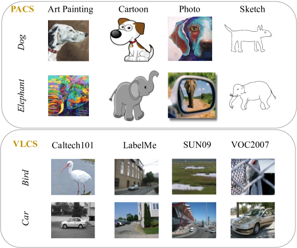
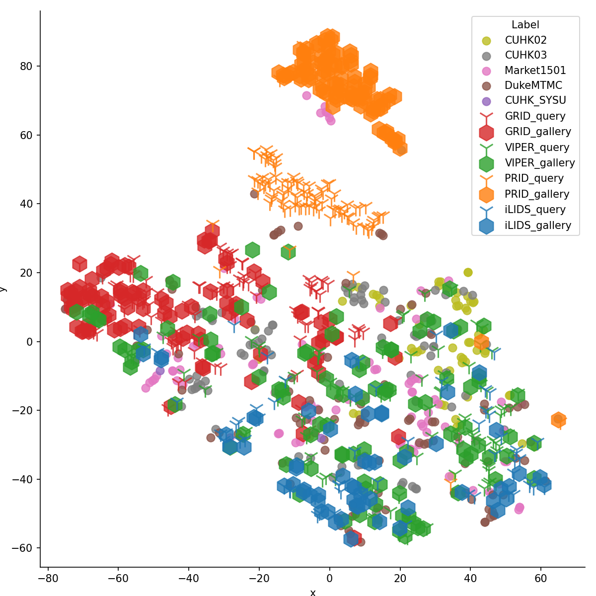
Refer to caption
Figure 6: Data examples from the PACS and the VLCS datasets.
Refer to caption
(a) ERM (All).
Refer to caption
(b) MetaBIN (All).
Refer to caption
(c) DANN+ELS (All).
Refer to caption
(d) ERM (Test)
Refer to caption
(e) MetaBIN (Test).
Refer to caption
(f) DANN+ELS (Test).
Figure 7: Visualization of the embeddings on training and test datasets. Query and gallery samples of these unseen datasets are shown using different types of mark. Best viewed in color.
Refer to caption
(a) Domain discrimination loss.
Refer to caption
(b) Identity classification loss.
Refer to caption
(c) Average m𝑚mAP on the test set.
Figure 8: Training statistics on ReID datasets.

D.3 Ablation Studies