Reanalysis of the X-ray burst associated FRB 200428 with Insight-HXMT observations
Abstract
A double-peak X-ray burst from the Galactic magnetar SGR J1935+2154 was discovered as associated with the two radio pulses of FRB 200428 separated by ms. Precise measurements of the timing and spectral properties of the X-ray bursts are helpful for understanding the physical origin of fast radio bursts (FRBs). In this paper, we have reconstructed some information about the hard X-ray events, which were lost because the High Energy X-ray Telescope (HE) onboard the Insight-HXMT mission was saturated by this extremely bright burst, and used the information to improve the temporal and spectral analyses of the X-ray burst. The arrival times of the two X-ray peaks by fitting the new Insight-HXMT/HE lightcurve with multi-Gaussian profiles are ms and ms after the first peak of FRB 200428, respectively, while these two parameters are ms and ms if the fitting profile is a fast rise and exponential decay function. The spectrum of the two X-ray peaks could be described by a cutoff power-law with cutoff energy keV and photon index , the latter is softer than that of the underlying bright and broader X-ray burst when the two X-ray peaks appeared.
1 Introduction
Fast radio bursts (FRBs) are the brightest flashes in the radio sky (Petroff et al., 2019; Cordes & Chatterjee, 2019). However, their physical mechanism has remained mysterious so far (Zhang, 2020; Xiao et al., 2021), although the discovery of FRB 200428 establishes magnetars as an origin of some FRBs (Bochenek et al., 2020; CHIME/FRB Collaboration et al., 2020). At the same time, its X-ray counterpart, a bright X-ray burst (XRB), was detected by high energy instruments such as Insight-HXMT, INTEGRAL, Konus-Wind, and AGILE (Li et al., 2021; Mereghetti et al., 2020; Ridnaia et al., 2021; Tavani et al., 2021). Insight-HXMT discovered the double X-ray peaks corresponding to the double radio peaks (Li et al., 2021), and both Insight-HXMT and INTEGRAL localized the X-ray burst as coming from SGR J1935+2154 (Li et al., 2021; Mereghetti et al., 2020). It is the first time that a counterpart of an FRB was detected and localized at other wavelengths, which allowed the identification of the origin of an FRB (Palm, 2022; Enoto et al., 2022; Roberts et al., 2022; Li et al., 2022a).
Since October 2022, SGR J1935+2154 went into a new active episode (Palm, 2022; Enoto et al., 2022; Roberts et al., 2022; Li et al., 2022a). After the burst forest, at least two FRB signals were captured by CHIME (Dong & Chime/Frb Collaboration, 2022), GBT (Maan et al., 2022) and Yunnan 40 m radio telescope (ATEL 15707) and their corresponding X-ray burst are detected by GECAM, HEBS(GECAM-C), Konus-Wind and Insight-HXMT (Wang et al., 2022; Frederiks et al., 2022; Li et al., 2022b). Compared to these results, more constraints on the FRB mechanism could be supplied by the timing properties of FRB 200428 and XRB, such as the time delay and the quasi-period oscillation in XRB (Li et al., 2021; Ridnaia et al., 2021; Mereghetti et al., 2020; Li et al., 2022). In the previous study, marginal time delay in the XRB lightcurves has been detected by Insight-HXMT, especially for the second peak (Li et al., 2021). Mereghetti et al. (2020) also report that there is a hard X-ray time delay of ms for the second peak. Until now, no more measurements have been reported for the timing properties between FRB 200428 and the XRB. We have recovered some of the hard X-ray events of this XRB, which were lost because the High Energy X-ray Telescope (HE) onboard the Insight-HXMT mission was saturated by this extremely bright burst. Here, we utilize the recovered data of Insight-HXMT/HE together with Insight-HXMT/ME, INTEGRAL and Konus-Wind to perform a detailed timing analysis for the double-peak structure of the XRB by fitting its lightcurve.
2 Observations and Data processing
Insight-HXMT is China’s first X-ray astronomical satellite, which carries three main payloads: the High Energy X-ray telescope (HE, 20-250 keV, 5100 cm2), the Medium Energy X-ray telescope (ME, 5-30 keV, 952 cm2), and the Low Energy X-ray telescope (LE, 1-15 keV, 384 cm2) (Li & Wu, 1993; Li et al., 1993; Zhang et al., 2014, 2020; Liu et al., 2020; Cao et al., 2020; Chen et al., 2020). Insight-HXMT was in pointing observation mode and acquired high quality data when FRB 200428 occurred. The data supply a unique opportunity to study the timing properties of the FRB event in X-ray energy band. The Insight-HXMT observation ID including the XRB corresponding to FRB 200428 is P0314003001. The data process of XRB is similar to the procedure described as in Li et al. (2021), which only used the recovered lightcurve of one third of the detectors of Insight-HXMT/HE (HE for clarity, hereafter). In this work, all the detectors of HE are used to perform timing analysis. The results of Insight-HXMT/ME (ME for clarity, hereafter) are obtained from Li et al. (2021) directly. However, the results of Insight-HXMT/LE (LE for clarity, hereafter) are not utilized here as the first peak is not detected in LE lightcurve (Li et al., 2021).
HE consists of eighteen phoswich X-ray detectors. These detectors are divided into three groups. Each group contains six detectors sharing one Physical Data Acquisition Unit (PDAU for short). Each PDAU contains a FIFO with 9-bit width and 2048-byte depth acting as data buffer. A half-full flag will be set when 1024 bytes data are written into the FIFO. Then the PDAU will read out and transfer these data to the solid storage device of the satellite platform. This operation takes about 7 ms. When HE observes a burst with extremely high flux, the FIFO will rapidly be filled up in less than 7 ms. Then part of the data can not be recorded and will be lost. It results in some gaps in the original lightcurve of HE. This is the so-called saturation effect in HE. As mentioned by Li et al. (2021), the XRB corresponding to FRB 200428A saturated HE seriously. It would affect the timing properties and needs to be corrected. Fortunately, with a deep understanding of the working mechanism of PDAU, we can accurately estimate the average count rate during the gaps in the lightcurve where the event data are lost. Even though we can not recover the lost data event by event, the recovered count rate data points can fill the gaps in the lightcurve and significantly improve the quality of the lightcurve. The saturation and deadtime corrections for all HE data consists of several major steps: (1) recover the data points with average count rate with raw data (level 1B data for HE); (2) find the time intervals where no raw data is lost; (3) obtain the deadtime ratio of each detector at different time intervals; (4) screen the data in the time intervals selected in the first step and then calculate the true count rate of each detector; (5) merge these count rates and calculate their errors. As shown in Figure 1, the lightcurves obtained from the three groups of detectors are utilized to analyse the timing parameters and the systematic error is set to 0.06 for the light curves, according to their different responses and backgrounds of these HE detectors (Li et al., 2020; Liao et al., 2020). The lightcurves for different energy bands could be generated from similar procedure as described in Li et al. (2021).
After saturation and deadtime corrections, three lightcurves of HE, one in the whole energy band (15–250 keV) and two narrower energy bands (15–60 keV and 60–250 keV), are recovered as shown in Figures 1, 2 and 3, which display more detailed structures than the ones without correction as shown in Li et al. (2021). The two hard X-ray bursts associated with FRB 200428 are more significant in the HE lightcurves than that in the previous results.
3 Timing and spectral analysis
3.1 Lightcurve fitting
We utilize several Gaussian functions to fit the three lightcurves of HE to calculate their timing properties as proposed in Li et al. (2021). In order to describe the timing properties of FRB 200428 and the XRB conveniently, all arrival times are set relative to 2020-04-28T14:34:24.4265 (UTC, geocentric), corresponding to the first peak of FRB 200428 (CHIME/FRB Collaboration et al., 2020). As shown in Figures 2 and 3, the structures of HE lightcurve in energy band 60–250 keV are less than that in energy bands 15–60 keV and 15–250 keV. Briefly, we take the HE lightcurve in energy band 15–250 keV as an example to describe the fitting process.
As plotted in Figure 2, the HE lightcurve in energy band 15–250 keV consists of three broad bump-like components and two narrow peaks, corresponding to the two radio bursts of FRB 200428. Except for these five components, there are two other weaker peaks (with less significance) before the two narrow peaks. For convenience, we name the two FRB peaks and the corresponding X-ray peaks as and . The two weaker peaks are named as and while the three broad bump-like components are named as to as listed in Table 1. However, we only focus on the timing properties of and and the other five components are not discussed further in this work.
To describe these components, we fit the HE lightcurve with seven Gaussian functions and a constant term, which are used to describe to ,
| (1) |
where . , , , , and are the coefficients, the arrival times and Gaussian widths of and detected by HE, respectively. is the sum of the five Gaussian functions for describing the two small structures and three broad bump-like components of the lightcurve located at around , , , and , respectively. The last term is the background of the lightcurve.
As shown with the green line in Figure 2, the HE lightcurve can be well fitted by equation (1). The parameters of the best fitting are listed in Table 1 with a reduced of 1.45 for 290 degrees of freedom.
The fitting process of the HE lightcurve in energy band 15-60 keV is the same as described above. However, the two components and are not present when fitting the HE lightcurve in energy band 60–250 keV as shown in Figure 3(b). The fitting parameters and goodness for these two lightcurves are also listed in Table 1.
The burst shape of FRB 200428 is typically asymmetric with a fast rise and a slow decay. Here, we also utilize a common form called the fast-rising exponential decay (FRED, Norris et al. (1996)) to replace the Gaussian functions for and as follows
| (2) |
, where is the normalization parameter, is the peak time, and are the rise and decay time constants, is the sharpness of the pulse for each time bin. The fitting parameters and goodness for these two lightcurves are also listed in Table 2. Limited by the data quality, only the lightcurves of Insight-HXMT/HE can be fitted with FRED functions.
3.2 Calculation of timing parameters
To quantify the timing properties of FRB 200428 and the XRB, the arrival times of all peaks, the time delays between radio peaks and X-ray peaks, peak separation for radio peaks or X-ray peaks are calculated in this work. The arrival times have been obtained by fitting the HE lightcurve, as listed in Tables 1 and 3. We also utilize the results from CHIME, ME and INTEGRAL and Konus-Wind, which are obtained from the literature (CHIME/FRB Collaboration et al., 2020; Li et al., 2021; Mereghetti et al., 2020; Ridnaia et al., 2021). For clarity, we denote and as the arrival time of the two peaks, where FRB, HE, ME, KW, IN or X to represent FRB 200428, HE, ME, Konus-Wind, INTEGRAL/IBIS or XRB. Here X represents the weighted mean value for the X-ray results obtained from different X-ray telescopes. After that, the time delays between radio and X-ray peaks are calculated as and , respectively. At the same time, the peak separations for radio or X-ray peaks are calculated with , where represents the same meanings. Finally, the difference between radio peak separation and X-ray peak separation is obtained as . The pulse width is defined as the full width at half maximum of the peak. In the end, the values of these parameters are summarised and listed in Table 3.
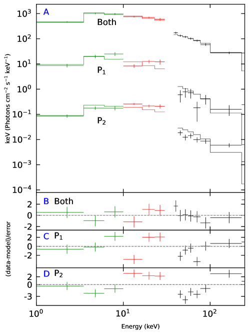
3.3 Spectra of the two narrow peaks
In order to obtain the spectra of the and individually and combined, we subtract the background using the background algorithm implemented within the RMFIT and GRM data tool 111https://fermi.gsfc.nasa.gov/ssc/data/analysis/software/. Taking HE as an example, the estimation procedure of the background of HE is described as follows: (1) extract the lightcurve for the specific channel; (2) exclude the the time interval of and ; (3) fit the rest lightcurve with Gaussian functions as background; (4) calculate the background for the selected channel. The net spectra of LE and ME are extracted similarly. Finally, the net spectra of , and both of them are fitted with cons*TBabs*cutoffpl and pgstat statistics in XSPEC as Li et al. (2021). In the fitting process, constant factors are added to implement the different saturation and deadtime effects in different detectors (Li et al., 2021). Because of the low statistics, we fix the constant factors of and to the values derived from the joint fitting of both peaks. The spectral results can be found in Figure 6 and the best fitting parameters are listed in Table 4.
4 Results and discussions
The timing parameters measured from different instruments or in different energy bands are plotted in Figure 5. The timing parameters do not show significant evolution as function of energy according to the energy coverage and uncertainties. Considering these factors, the timing parameters could be combined to reduce the statistical errors.
As listed in Table 3, the values of the arrival time measured from HE, ME, Konus-Wind and INTEGRAL are ms, ms, ms, and ms, respectively (Ridnaia et al., 2021; Mereghetti et al., 2020). By combining the four arrival times with a weighted average, we obtain ms. Similarly, we obtain ms from the combined X-ray observations as listed in Table 3. According to the arrival times of radio emission (CHIME/FRB Collaboration et al., 2020), we can obtain the time delays of the two X-ray peaks as ms and ms, respectively. It is the first time that the delay of the X-ray emission of relative to the first radio burst is obtained with a high confidence level of . We also confirm that the X-ray emission of delays relative to the second radio peak at an even higher confidence level than the previous results, which is longer than that of (Li et al., 2021; Ridnaia et al., 2021; Mereghetti et al., 2020).
The separation of the two X-ray peaks is ms, which is longer than the radio peak separation of ms detected by CHIME/FRB (CHIME/FRB Collaboration et al., 2020). Hence, the difference between the radio peak separation and the X-ray peak separation is ms, which is above zero at 4.3 significance level and is also more significant than that reported in previous results (Li et al., 2021; Ridnaia et al., 2021; Mereghetti et al., 2020). We conclude that there is a difference in the observed peak separations between the two bursts of the FRB and its X-ray counterpart.
As shown in the right panels of Figures 2, 3 and 4, and could be also well fitted by a FRED function for the three lightcurves with energy bands 15-250 keV, 15-60 keV and 60-250 keV. The timing parameters do not evolve with energy from the FRED fitting results and similar with the results fitting with multi-Gaussian functions as listed in Table 2. Considering these factors, the timing parameters are only discussed for the whole energy band of Insight-HXMT/HE. With the timing parameters of FRED function, the X-ray peak of is definitely delayed by about ms while shows longer delay of ms. The separation between the two X-ray peaks is ms, which is roughly consistent with as this value is somewhat model (Gaussian or FRED) dependent. Interestingly, in the 60-250 keV band, one can also get ms from the FRED fitting result. Within the margin of error, this value agrees with that of ms obtained from the multi-Gaussian fitting result.
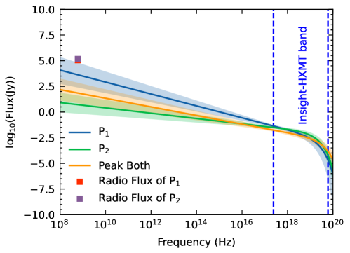
We also obtained the detailed spectral information of and as shown in Figure 6 and Table 4. From the fitting results, the photon index of the combined spectrum of and is softer than the previous result of of the spectrum including both the two bursts and the broader components of the burst in the same time interval when the two bursts occurred (Li et al., 2021). The cutoff energy is consistent with the previous result within errors. In addition, the photon index and cutoff energy of are consistent with as listed in Table 4. Finally, the radio fluxes are higher than that extrapolated from X-ray spectral parameters as shown in Figure 7 (Li et al., 2021; CHIME/FRB Collaboration et al., 2020).
Many recent theoretical models attribute FRBs and XRBs to various sorts of instablities in the magnetar’s magnetosphere (Wu et al., 2020; Margalit et al., 2019; Xiao & Dai, 2020; Margalit et al., 2020; Yu et al., 2021; Yuan et al., 2020; Wadiasingh & Timokhin, 2019; Kumar & Bošnjak, 2020; Yang et al., 2020; Lu et al., 2020; Yang & Zhang, 2021; Dai, 2020; Geng et al., 2020). In these scenarios, the instabilities are triggered by perturbations in a certain critical condition somewhere in the magnetosphere where FRBs and XRBs are emitted. Indeed, these scenarios can be appllied in the most general cases, although there may be differences in the origin between various trigger mechanisms.
In general, the observed time delay between any two burst events and can be given by
| (3) |
where and are the distances of the emitting points to the observer on the Earth, and and are the moments when the bursts emerge. Here, and can be regarded as the two peaks in the XRB. There may be three possibilities. First, if the two events are caused by individual perturbations successively occurred at the same place or in a very small area, the time interval of the two events dominates the time delay, for the XRB. Similarly, we have for the FRB. Second, the two emission events may be thought of as originated from the same perturbation with two pulses. In this case, the time delay between the radio and X-ray peaks is dominated by perturbation propagation if we suppose that the propagation speed is much less than the light speed. We have . Third, it is also possible that the two burst events corresponding to the two peaks in the XRB/FRB occur independently in two fairly distant places. In this case, the two burst events are totally incidental coincidence in tens of milliseconds.
From the results of timing analysis, we can conclude that the first X-ray peak is delayed by about 3 ms relative to the first peak of FRB 200428. The separation between the two X-ray peaks may or may not show significant difference with the separation of the two radio peaks of FRB 200428, depending on which model (Gaussian or FRED) is applied in fitting the lightcurves of the two X-ray peaks. On the other hand, the time-resolved spectral analysis shows that there are no significant differences in the spectral parameters of the two XRB sub-bursts and , such as the photon index , and cutoff energy keV, which indicates the same origin for the two sub-bursts. Actually, the spectral parameters of the two sub-bursts in the XRB are also consistent with the trend of the overall spectral evolution during the XRB (Li et al., 2021; Mereghetti et al., 2020; Ridnaia et al., 2021).
Combining the results of timing analysis and spectral analysis, it is very likely that the two sub-bursts and of FRB 200428 and its associated XRB should originate from the same circumburst environment, or be affected by the same environmental factors. We thus suggest that the FRB and XRB originated from the same perturbation with two sub-bursts, emitting radio and X-ray at different places satisfying the respective critical condition of instability in the propagation of the perturbation, as the second case discussed above.
5 Summary
In this work, we present a more detailed timing analysis to the lightcurves of Insight-HXMT/HE observation of the XRB associated with FRB 200428 after the saturation corrections. The arrival times of the two X-ray peaks by fitting the lightcurve with multi-Gaussian functions are ms and ms, which are much more accurate than the previous results. Together with the results of Insight-HXMT/ME, INTEGRAL and Konus-Wind, the weighted mean time delays of the two X-ray peaks corresponding to radio peaks are ms and ms, respectively. Then, we also obtained the peak separation between the two X-ray peaks of ms, which is longer than that of the two radio peaks of FRB 200428 with ms. At the same time, the lightcurve of Insight-HXMT/HE is fitted with an FRED function since the peak shape is asymmetric. According to FRED fitting results, the time delays of two X-ray peaks are ms and ms while the peak separation is equal to or greater than the separation of the two radio peaks, which is model dependent. In addition, these parameters do not show significant evolution with energy considering their errors. Finally, the spectrum of the two X-ray peaks are similar, which could be fitted by cutoff power-law with photon index and cutoff energy keV. These results could supply more constraints on the emission models of FRBs.
Acknowledgments
This work is supported by the National Key R&D Program of China (2021YFA0718500) from the Minister of Science and Technology of China (MOST). The authors thank supports from the National Natural Science Foundation of China under Grants 12173103, U2038101, U1938103 and 11733009. This work is also supported by International Partnership Program of Chinese Academy of Sciences (Grant No.113111KYSB20190020).
| Peak No. | Parameters | All | 15–60 keV | 60–250 keV |
|---|---|---|---|---|
| ( cnts/s) | ||||
| (ms) | ||||
| (ms) | ||||
| ( cnts/s) | ||||
| (ms) | ||||
| (ms) | ||||
| ( cnts/s) | ||||
| (ms) | ||||
| (ms) | ||||
| ( cnts/s) | ||||
| (ms) | ||||
| (ms) | ||||
| ( cnts/s) | ||||
| (ms) | ||||
| (ms) | ||||
| ( cnts/s) | ||||
| (ms) | ||||
| (ms) | ||||
| ( cnts/s) | ||||
| (ms) | ||||
| (ms) | ||||
| Bkg | ( cnts/s) | |||
| 1.45(290) | 1.56(290) | 1.58(296) |
| Peak No. | Parameters | All | 15–60 keV | 60–250 keV |
|---|---|---|---|---|
| ( cnts/s) | ||||
| (ms) | ||||
| (ms) | ||||
| (ms) | ||||
| ( cnts/s) | ||||
| (ms) | ||||
| (ms) | ||||
| (ms) | ||||
| ( cnts/s) | ||||
| (ms) | ||||
| (ms) | ||||
| ( cnts/s) | ||||
| (ms) | ||||
| (ms) | ||||
| ( cnts/s) | ||||
| (ms) | ||||
| (ms) | ||||
| ( cnts/s) | ||||
| (ms) | ||||
| (ms) | ||||
| ( cnts/s) | ||||
| (ms) | ||||
| (ms) | ||||
| Bkg | ( cnts/s) | |||
| 1.46(286) | 1.54(286) | 1.59(292) |
| Parameters | FRB(a) | HE(b) | ME(c) | KW(d) | IN(e) | X(f) | HE(g) |
|---|---|---|---|---|---|---|---|
| (ms) | |||||||
| (ms) | – | – | – | – | |||
| (ms) | |||||||
| (ms) | – | – | – | – | |||
| (ms) | |||||||
| (ms) | – | – | – | – | |||
| (ms) | – | – | – | – | |||
| (ms) | – | – | – | – |
(a) FRB 200428: CHIME/FRB Collaboration et al. (2020).
(b) Insight-HXMT/HE: parameters fitted by multi-Gaussian functions in this work.
(c) Insight-HXMT/ME: Li et al. (2021)
(d) INTEGRAL/IBIS: Mereghetti et al. (2020).
(e) Konus-Wind: Ridnaia et al. (2021).
(f) X: the weighted mean values of parameters obtained from several instruments mentioned above.
(g) Insight-HXMT/HE: parameters fitted by FRED function in this work
| Parameter | Both | ||
|---|---|---|---|
| Norm | |||
| PhoIndex | |||
| HighECut (keV) | |||
| Factor of HE | 0.4(fixed) | 0.4(fixed) | |
| Factor of ME | 1.0(fixed) | 1.0(fixed) | 1.0(fixed) |
| Factor of LE | 0.9(fixed) | 0.9(fixed) | |
| 14.8/9 | 38.1/10 | 57.9/10 |
References
- Bochenek et al. (2020) Bochenek, C. D., Ravi, V., Belov, K. V., et al. 2020, Nature, 587, 59, doi: 10.1038/s41586-020-2872-x
- Cao et al. (2020) Cao, X., Jiang, W., Meng, B., et al. 2020, Science China Physics, Mechanics, and Astronomy, 63, 249504, doi: 10.1007/s11433-019-1506-1
- Chen et al. (2020) Chen, Y., Cui, W., Li, W., et al. 2020, Science China Physics, Mechanics, and Astronomy, 63, 249505, doi: 10.1007/s11433-019-1469-5
- CHIME/FRB Collaboration et al. (2020) CHIME/FRB Collaboration, Andersen, B. C., Bandura, K. M., et al. 2020, Nature, 587, 54, doi: 10.1038/s41586-020-2863-y
- Cordes & Chatterjee (2019) Cordes, J. M., & Chatterjee, S. 2019, ARA&A, 57, 417, doi: 10.1146/annurev-astro-091918-104501
- Dai (2020) Dai, Z. G. 2020, ApJ, 897, L40, doi: 10.3847/2041-8213/aba11b
- Dong & Chime/Frb Collaboration (2022) Dong, F. A., & Chime/Frb Collaboration. 2022, The Astronomer’s Telegram, 15681, 1
- Enoto et al. (2022) Enoto, T., Hu, C.-P., Guver, T., et al. 2022, The Astronomer’s Telegram, 15690, 1
- Frederiks et al. (2022) Frederiks, D., Ridnaia, A., Svinkin, D., et al. 2022, The Astronomer’s Telegram, 15686, 1
- Geng et al. (2020) Geng, J.-J., Li, B., Li, L.-B., et al. 2020, ApJ, 898, L55, doi: 10.3847/2041-8213/aba83c
- Kumar & Bošnjak (2020) Kumar, P., & Bošnjak, Ž. 2020, MNRAS, 494, 2385, doi: 10.1093/mnras/staa774
- Li et al. (2022a) Li, C., Cai, C., Xiong, S., et al. 2022a, The Astronomer’s Telegram, 15698, 1
- Li et al. (2021) Li, C. K., Lin, L., Xiong, S. L., et al. 2021, Nature Astronomy, 5, 378, doi: 10.1038/s41550-021-01302-6
- Li & Wu (1993) Li, T.-P., & Wu, M. 1993, Ap&SS, 206, 91, doi: 10.1007/BF00658385
- Li et al. (1993) Li, T.-P., Wu, M., Lu, Z.-G., Wang, J.-Z., & Zhang, C.-S. 1993, Ap&SS, 205, 381, doi: 10.1007/BF00658978
- Li et al. (2020) Li, X., Li, X., Tan, Y., et al. 2020, Journal of High Energy Astrophysics, 27, 64, doi: 10.1016/j.jheap.2020.02.009
- Li et al. (2022b) Li, X., Zhang, S., Xiong, S., et al. 2022b, The Astronomer’s Telegram, 15708, 1
- Li et al. (2022) Li, X., Ge, M., Lin, L., et al. 2022, ApJ, 931, 56, doi: 10.3847/1538-4357/ac6587
- Liao et al. (2020) Liao, J.-Y., Zhang, S., Lu, X.-F., et al. 2020, Journal of High Energy Astrophysics, 27, 14, doi: 10.1016/j.jheap.2020.04.002
- Liu et al. (2020) Liu, C., Zhang, Y., Li, X., et al. 2020, Science China Physics, Mechanics, and Astronomy, 63, 249503, doi: 10.1007/s11433-019-1486-x
- Lu et al. (2020) Lu, W., Kumar, P., & Zhang, B. 2020, MNRAS, 498, 1397, doi: 10.1093/mnras/staa2450
- Maan et al. (2022) Maan, Y., Leeuwen, J. v., Straal, S., & Pastor-Marazuela, I. 2022, The Astronomer’s Telegram, 15697, 1
- Margalit et al. (2020) Margalit, B., Beniamini, P., Sridhar, N., & Metzger, B. D. 2020, ApJ, 899, L27, doi: 10.3847/2041-8213/abac57
- Margalit et al. (2019) Margalit, B., Berger, E., & Metzger, B. D. 2019, ApJ, 886, 110, doi: 10.3847/1538-4357/ab4c31
- Mereghetti et al. (2020) Mereghetti, S., Savchenko, V., Ferrigno, C., et al. 2020, ApJ, 898, L29, doi: 10.3847/2041-8213/aba2cf
- Norris et al. (1996) Norris, J. P., Nemiroff, R. J., Bonnell, J. T., et al. 1996, ApJ, 459, 393, doi: 10.1086/176902
- Palm (2022) Palm, D. M. 2022, The Astronomer’s Telegram, 15667, 1
- Petroff et al. (2019) Petroff, E., Hessels, J. W. T., & Lorimer, D. R. 2019, A&A Rev., 27, 4, doi: 10.1007/s00159-019-0116-6
- Ridnaia et al. (2021) Ridnaia, A., Svinkin, D., Frederiks, D., et al. 2021, Nature Astronomy, 5, 372, doi: 10.1038/s41550-020-01265-0
- Roberts et al. (2022) Roberts, O., Dalessi, S., & Malacaria, C. 2022, The Astronomer’s Telegram, 15672, 1
- Tavani et al. (2021) Tavani, M., Casentini, C., Ursi, A., et al. 2021, Nature Astronomy, 5, 401, doi: 10.1038/s41550-020-01276-x
- Wadiasingh & Timokhin (2019) Wadiasingh, Z., & Timokhin, A. 2019, ApJ, 879, 4, doi: 10.3847/1538-4357/ab2240
- Wang et al. (2022) Wang, C., Xiong, S., Zhang, Y., et al. 2022, The Astronomer’s Telegram, 15682, 1
- Wu et al. (2020) Wu, Q., Zhang, G. Q., Wang, F. Y., & Dai, Z. G. 2020, ApJ, 900, L26, doi: 10.3847/2041-8213/abaef1
- Xiao & Dai (2020) Xiao, D., & Dai, Z.-G. 2020, ApJ, 904, L5, doi: 10.3847/2041-8213/abc551
- Xiao et al. (2021) Xiao, D., Wang, F., & Dai, Z. 2021, Science China Physics, Mechanics, and Astronomy, 64, 249501, doi: 10.1007/s11433-020-1661-7
- Yang & Zhang (2021) Yang, Y.-P., & Zhang, B. 2021, ApJ, 919, 89, doi: 10.3847/1538-4357/ac14b5
- Yang et al. (2020) Yang, Y.-P., Zhu, J.-P., Zhang, B., & Wu, X.-F. 2020, ApJ, 901, L13, doi: 10.3847/2041-8213/abb535
- Yu et al. (2021) Yu, Y.-W., Zou, Y.-C., Dai, Z.-G., & Yu, W.-F. 2021, MNRAS, 500, 2704, doi: 10.1093/mnras/staa3374
- Yuan et al. (2020) Yuan, Y., Beloborodov, A. M., Chen, A. Y., & Levin, Y. 2020, ApJ, 900, L21, doi: 10.3847/2041-8213/abafa8
- Zhang (2020) Zhang, B. 2020, Nature, 587, 45, doi: 10.1038/s41586-020-2828-1
- Zhang et al. (2014) Zhang, S., Lu, F. J., Zhang, S. N., & Li, T. P. 2014, in Society of Photo-Optical Instrumentation Engineers (SPIE) Conference Series, Vol. 9144, Space Telescopes and Instrumentation 2014: Ultraviolet to Gamma Ray, ed. T. Takahashi, J.-W. A. den Herder, & M. Bautz, 914421, doi: 10.1117/12.2054144
- Zhang et al. (2020) Zhang, S.-N., Li, T., Lu, F., et al. 2020, Science China Physics, Mechanics, and Astronomy, 63, 249502, doi: 10.1007/s11433-019-1432-6