Fourier series weight in quantum machine learning

Abstract

In this work, we aim to confirm the impact of the Fourier series on the quantum machine learning model. We will propose models, tests, and demonstrations to achieve this objective. We designed a quantum machine learning leveraged on the Hamiltonian encoding. With a subtle change, we performed the trigonometric interpolation, binary and multiclass classifier, and a quantum signal processing application. We also proposed a block diagram of determining approximately the Fourier coefficient based on quantum machine learning. We performed and tested all the proposed models using the Pennylane framework.

KeyWords: Quantum Computing, Quantum Machine Learning, Fourier Series, QML, QSP, Interpolation, Regression model, quantum classifiers

I Introduction

The Fourier series is a mathematical tool that allows us to model any arbitrary periodic signal with a combination of sines and cosines. Its main advantage is that very little signal information is lost during the transformation from one domain to another. Indeed, this series does not exist for all signals (Dirichlet conditionsChaudhuri and Feireisl (2022)); however, in various fields and sectors, the Fourier series is the tool used to transform a signal from the time domain to the frequency domain, breaking it down into harmonically related sinusoidal functions.

In quantum computing and specifically in the branch of quantum machine learning (QML), a quantum model is described by a parametric function $f(x,\theta)$ subject to some independent variables $x$ that could be our input data and some parameters $\theta$ that help our function to attempt to generalize itself across the input data.

Taking this into account and knowing the tremendous impact that the Fourier series has on signal processing, it is therefore of great interest to analyze and experiment to see how the Fourier series impacts the quantum models thus, if it could help us in quantum trigonometric interpolation techniques, regression models, etc.

In this article, we will highlight the importance of the Fourier series in solving real problems with quantum machine learning. We will also propose a generic quantum circuit that, with little change, can help us solve classification problems, interpolation for banking problems, and signal processing, among others.

The document is organized as follows. Section (II) presents our primary motivation behind this work. Section (III) shows previous work on Fourier series based quantum machine learning and the simulation of the dynamical behavior of a system. Section (IV) will present the quantum machine learning framework and its connection to the Hamiltonian simulation. In section (V), we propose the scenarios and the models we will implement to highlight the Fourier Series on quantum machine learning applications. Section (VI) analyses our model, taking into account some steps from the quantum model’s universality. Section (VII) presents the obtained results. Section (VII.1) discusses practically relevant results and their implications, and finally, Section (VIII) concludes the work carried out, and we open ourselves to some future lines of the proposed model.

II Motivation

Our primary motivation is to understand very well the QML model as a Fourier series to join the area of digital signal processing with quantum computing, both analytically and statistically, which is part of quantum machine learning.

III Related Work

In quantum computing, one of the most demanding problems is the simulation of the Hamiltonian. Hamiltonian simulation is a problem that requires algorithms that efficiently implement a quantum state’s evolution. Richard Feynman proposed the Hamiltonian simulation problem in 1982, where he proposed a quantum computer as a possible solution since the simulation of general Hamiltonians seems to grow exponentially concerning the size of the system. Nowadays, this problem is reflected in almost all the systems under study, where we want to analyze the physical design and dynamics within a computational model.

The Hamiltonian simulation problem is defined by the Schrödinger equation, where it gives a Hermitian matrix $H(2^{n}\times 2^{n})$ that acts on $n$ qubits in a time $t$ and a maximum simulation error $(\epsilon)$, whose goal is to find an algorithm that approximates an operator $U$ such that $||U-(e^{-iHt})||\leq\epsilon$. Where $e^{-iHt}$ is the ideal evolution.

The quantum simulation of the dynamical behavior of a system is usually executed in polynomial time $P$, $BQP$, etc. But its Hamiltonian matrix grows exponentially $2^{n}\times 2^{n}$ relating to the $n$ qubits of the systems under study. Thus, techniques are sought to tackle the best solution assuming an error. There are two strategies, Julius Caesar (divide and conquer) and the quantum walk algorithmAmbainis (2007); Schuld and Petruccione (2018). A helper is a Local Hamiltonian for some specific Hamiltonians. A k-local Hamiltonian Kempe et al. (2006) is a Hermitian matrix acting on $n$ qubits that can be represented as the sum $m$ of the Hamiltonian terms acting on each of the qubits at most: $H=\sum_{i}H_{i}$. This also gives rise to d-sparse Childs and Kothari (2010). A Hamiltonian is said to be d-sparse (on a fixed basis) if it has at most $d$ nonzero entries in any row or column.

From the Divide and conquer, the first step breaks down the Hamiltonian into a sum of small and straightforward Hamiltonians, and the second step has the objective of recombining the sums of small and straightforward Hamiltonians. To do this, there are three great techniques.

1. The first technique is one of the mature approaches, which is $e^{-i(A+B)t}$ where $A$ and $B$ are the small and straightforward Hamiltonians in an approximation of ($e^{-iAt/r}e^{-iBt/r})^{r}$ for large a real value $r$ Hatano and Suzuki (2005).

2. The second technique combines a Linear Combination of Unitaries (LCU)Meister et al. (2022); Wang et al. (2021); Alonso-Linaje and Atchade-Adelomou (2021) and the Oblivious Amplitude Amplification (OAA) De Raedt and De Raedt (1983); Guerreschi (2019); Novo and Berry (2016).

3. The latest newest technique is the Quantum Signal Processing (QSP) Eldar and Oppenheim (2002); Silva et al. (2022).

In contrast, computing a system’s ground state energy optimizes a given system’s global property. Usually, this problem is very demanding (NP-Hard). The most known problem is calculating the minimum expectation value of a quantum circuit $\langle\phi|H|\phi\rangle$ overall $|\phi\rangle$.

There are two ways to solve this problem using the Top-Down philosophy and statistical methods. On the one hand, the Top-Down is where analytical techniques are applied. On the other, statistical methods (like QML) are sought through the variational principle, where a model approximates the solution. This paper will focus on the second case and highlight the relationship between the two resolution approaches.

The use of the quantum model as a Fourier series has already been studied in these papers Du et al. (2020); Schuld et al. (2021). There have been much more works Pérez-Salinas et al. (2020); Killoran et al. (2019); Sim et al. (2019); Chen et al. (2021); Du et al. (2020); Biamonte (2021) on the techniques relevant to the approach we chose Schuld et al. (2021), where the authors defined an exciting framework to establish the intuitions. However, given how challenging the topic is, the authors described some interesting practical ideas for QSP and quantum machine learning on the data in search of some advantages. Therefore, in this article, first, we want to confirm that quantum models naturally learn periodic patterns in data. Second, see the natural representation of the Fourier series to study time series learning and signal processing tasks as necessary applications based on trigonometric interpolation suitable for quantum machine learning. Third, experiment and propose the quantum circuit as a neural network that, with a few changes, can be used as an interpolation and classifier model.

IV Quantum Machine Learning

Quantum machine learning (QML) Schuld et al. (2015); Biamonte et al. (2017); Schuld and Petruccione (2018) explores the interplay and takes advantage of quantum computing and machine learning ideas and technics.

Therefore, quantum machine learning is a hybrid system involving both classical and quantum processing, where computationally complex subroutines are given to quantum devices. QML tries to take advantage of the classical machine learning does best and what it costs, such as distance calculation (inner product), passing it onto a quantum computer that can compute it natively in the Hilbert vector space. In this era of large classical data and few qubits, the most common use is to design machine learning algorithms for classical data analysis running on a quantum computer, i.e., quantum-enhanced machine learning Dunjko et al. (2016); Atchade Adelomou et al. (2020); Atchade-Adelomou and Alonso-Linaje (2022); Adelomou et al. (2022); Guillermo (2023); Schuld and Petruccione (2018). The usual supervised learning processes within quantum machine learning can be defined as follows:

• The quantum feature map: It is the data preparation. In the literature, this stage is recognized as State preparation.

• The quantum model: It is the model creation. In the literature, it is recognized as unitary evolution.

• The classical error computation : It is the stage of computing the error where the model best approximates the input set; in machine learning, this stage is known as prediction.

• Observable: Normally, this stage is included in the error computation. The observable manifest as linear operators on a Hilbert space represents quantum states’ state space. The eigenvalues of observable are real numbers corresponding to possible values; the dynamical variable defined by the observable can be measured. We use Pauli’s operators as observable. Nevertheless, we can use some linear combination (6) of these operators or some approximation (7) from them to deal with specific measurements.

IV.1 Feature Map

This article deals exclusively with classical data; we receive classical data, and a quantum computer processes it and returns the outcome after the measurement. There are other (three additional) different approaches and combinations to process classical or quantum data with hybrid computation Schuld and Petruccione (2018). In quantum machine learning techniques, some fundamental operations called embedding are performed to treat classical data. The embedding process is summarized as classical encoding inputs into quantum states. In the literature, several techniques and their relative associated computational costs are found in these references Havlíček et al. (2019); Schuld and Petruccione (2018); Schuld et al. (2021); Schuld and Killoran (2019); Pérez-Salinas et al. (2020). We call the Feature Map the container carrying out said mapping operation (embedding). The embedding encoding can be amplitude, phase, base, or Hamiltonian, which is the crucial process of QML operations Schuld and Petruccione (2018).

This work follows the data encoding Hamiltonians idea, which is described as follows: For any unitary matrix $A$, there is a real vector $(\alpha,\beta,\gamma,\delta)$ such that $A=\alpha I+\beta X+\delta Y+\gamma Z$. For large enough $r$, the following equation holds $e^{-i(H_{A}+H_{B})t}\approx(e^{-iH_{A}t/r}e^{-iH_{B}t/r})^{r}$ using the Trotter Suzuki formula De Raedt and De Raedt (1983) which implies that if $r$ scales as $m^{2}t^{2}/\epsilon$, the error can be at most $\epsilon$ for any $\epsilon>0$.

More accurate approximations can be generated by constructing a sequence of exponential operators such that the error terms cancel. The most straightforward formula, which is the second-order Trotter Suzuki formula Wittek and Cucchietti (2013), takes the form as follows:

$$U_{2}(t):=\left(\prod_{j=1}^{m}e^{(-iH_{j}\frac{t}{2r})}\prod_{j=1}^{m}e^{(-iH_{j}\frac{t}{2r})}\right)^{r},$$ (1)

where the error can be given to less than $\epsilon$ for any $\epsilon>0$ when choosing $r$ to scale as $m^{3/2}t^{3/2}/\sqrt{\epsilon}$.

One of the alternative ways to encode the data is by amplitude into a quantum state given by complex continuous data represented as complex values $\bm{A}\in\mathbb{C}^{2^{N}}$:

$$\bm{A}=(a_{0},\ldots,a_{2^{N}-1})\mapsto\sum_{k=0}^{2^{N}-1}a_{k}|k\rangle,$$ (2)

with:

$$\lVert\bm{A}\rVert=1.$$ (3)

In the typical design of the quantum model (see Figure (1)), the feature map is usually seen fixed as the only block at the beginning of the quantum circuit and without repetition. Said design/strategy does not help the quantum model generalize the parameterized function better as a neural network, and our proposed model will strongly consider this fact.

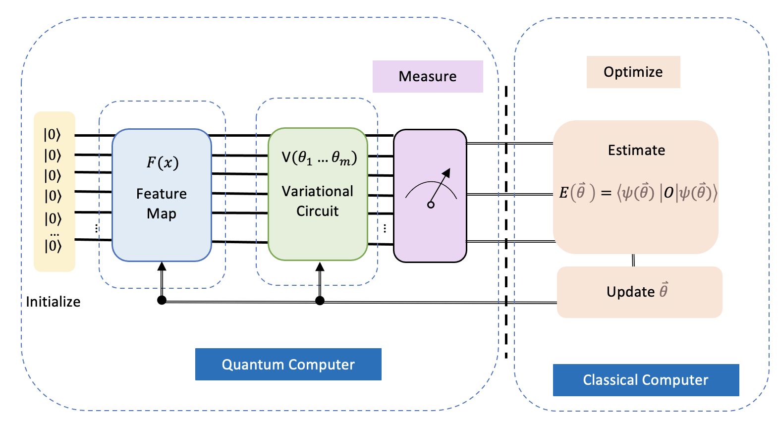
Figure 1: This figure is the standard quantum machine learning model in the literature with only one embedding block and an Ansatz as a parameterized quantum circuit with $m$ parameters. This model has a limitation: in the worst case, when the input data is not very well coded, for many parameters $m$ we add to our parametric function/circuit, we cannot find the best model that generalizes the input data. There have been various design proposals for how a quantum circuit should be Lloyd et al. (2020); Suzuki et al. (2020); Schuld and Killoran (2019).

IV.2 The model

This paper focuses on supervised learning applications to drive this section. Quantum models are parameterizable univariate or multivariate functions. The quantum gates that help to define the parameterizable functions are $RX$, $RY$, and $RZ$. Considering a quantum computer is a stochastic machine, to have a deterministic quantum model, the output of our model must be an expected value (here, considering the computation basis $p(0)-p(1)$). That is, we must average the stochastic quantum computer’s outcome. An example of a quantum model is given as follows:

$$f_{\bm{\theta},\bm{\beta}}(x)=\bra{0}U^{\dagger}(\vec{x},\beta,\vec{\theta})OU(\vec{x},\beta,\vec{\theta})\ket{0},$$ (4)

Where $O$ is our observable, $U(\vec{x},\beta,\vec{\theta})$ the parameterized circuit with the input data $\vec{x}$, $\beta$, the scaling factor and $\vec{\theta}$, the parameterized variable.

IV.3 The error calculation

The error analysis of a QML is identical to the phases of the classical machine learning process. Error analysis allows us to know how to improve the performance of our quantum model. Equation (5) helps to analyze the training errors.

$$q\_err=\sqrt{\left(\frac{1}{n}\right)\sum_{i=1}^{n}(q\_model(\vec{x},\theta_{i})-Label_{i})^{2}}$$ (5)

IV.4 The Observable

In a quantum circuit, the observable determines the form and the function’s degree we use to classify or interpolate. For example, in the case of linear classification, the observable defines the linear form that the model will try to adapt to the input data better.

In our case, we use the computational basis $Z$. However, we can use the observable, such as above mentioned:

$$O=\sum_{P\in\{I,X,Y,Z\}^{\otimes n}}\alpha_{p}P,$$ (6)

and

$$O^{\text{(low)}}=\sum_{|P|\leq k}\alpha_{p}P.$$ (7)

V IMPLEMENTATION

The scenarios we follow to validate our experimentation are given in figure (2). The first scenario is a univariate function. This function will be a sine, a cosine, a logarithm, and a rectangular pulse. The second scenario is a multivariate function that is an arithmetic operation on $m$ univariate functions. The third scenario is where the input data is regrouped in a classical dataset. Said dataset results from a study on classical machine learning models and statistical events. However, the data can be from any analysis, even if quantum processes after being observed.

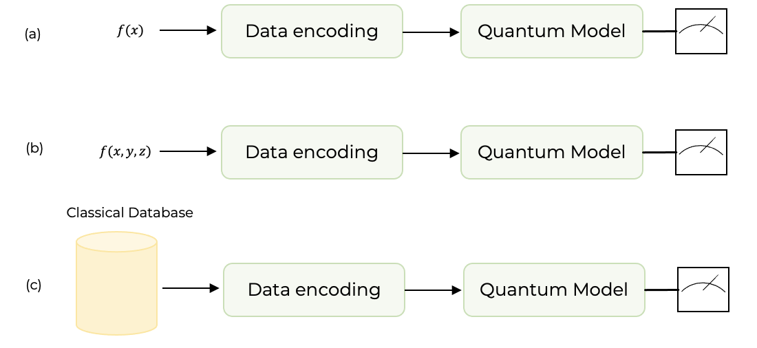
Figure 2: Scenario (a) will be a univariate function. This function will be a sine, a cosine, a logarithm, and a rectangular pulse. Scenario (b) is a multivariate function that can be an arithmetic operation on $m$ univariate functions. Scenario (c) is where the input data is regrouped in a classical dataset. Said dataset is the result of a study on classical machine learning models. However, the data can be from any analysis, even if quantum processes after being observed.

V.1 OUR QUANTUM MODEL

Based on the following work Schuld et al. (2021), where the authors studied the expressivity of the quantum model with a Pauli-rotation and later extended their study in the generality of the quantum model as a Fourier series, we aim to extend said the investigation into a demanding quantum circuit for machine learning. To realize our study, we have defined a quantum variational Feature Map together with a quantum variational circuit that, taking advantage of its mixture, can behave like a proper quantum neural network and, then verify the Fourier series’ weight in those quantum models (see Figure (3)). With a few subtle changes in the created quantum model, we have performed regression operations, classifications, and trigonometric interpolation. Let $F(\vec{x},\beta_{i})$ be our feature map and $V(\vec{\theta}_{i})$ be the variational quantum circuit, so the proposed model can be written as follow:

$$U(\vec{x},\beta,\vec{\theta})=F(\vec{x},\beta)V(\vec{\theta}),$$ (8)

where $\vec{x}$ is the input data, $\beta$, the scaling factor, and $\vec{\theta}$ the parameter.

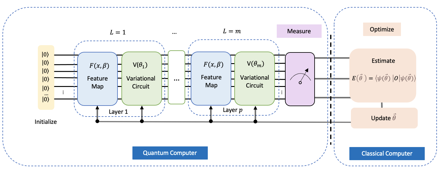
Figure 3: This is the model we use to analyze the weight of the Fourier series in quantum machine learning. Depending on some scaling parameters $\beta$ and the input data $\vec{x}$, the Feature Map will be in charge of coding our data. We rely heavily on the fact that the Feature Map ($F(\vec{x},\beta)$) must be variational, that the data’s loading is repeated in all the layers, and that the variational circuit ($V(\vec{\theta})$) searches the best function within the space of functions that defines the capacity of the variational circuit ($U(\vec{x},\beta,\vec{\theta})=F(\vec{x},\beta)V(\vec{\theta)}$). With this configuration, we get closer to a quantum neural network that interpolates like a trigonometric function or classifies depending on the problem.

VI FOURIER SERIES BASED ON QUANTUM CIRCUIT

In this session, we recover the work Schuld et al. (2021) on the quantum model’s universality and will adapt it to our case.

Based on Schuld et al. (2021); Gil Vidal and Theis (2020), where the authors demonstrated the universality of their theorem, considering the multivariate function of equation (4). We follow the steps described in said work and confirm that $f(x)$ follows the Fourier series decomposition for one layer. For that, let us recall the equation (4), which adapts it to the definition of the proposed feature map $F(\vec{x},\beta)$ and variation quantum circuit $V(\vec{\theta_{i}})$ as follow.

$$f(x)=\bra{0}U^{\dagger}(\vec{x},\vec{\theta},\beta)OU(\vec{x},\vec{\theta},\beta)\ket{0},$$ (9)

where

$$U(\vec{\theta},\beta,\vec{x})=V^{(2)}(\vec{\theta}^{(2)})F(\vec{x},\beta)V^{(1)}(\vec{\theta}^{(1)}),$$ (10)

with $\vec{\theta}^{(1)},\vec{\theta}^{(2)}\subseteq\vec{\theta}$ and recalling the equation (8), we can re-write it as follows:

$$F(\vec{x},\beta)=e^{-ix_{1}\beta H_{1}}\otimes\ldots\otimes e^{-ix_{N}\beta H_{N}}.$$ (11)

If we make the assumption that $H_{p}$ is diagonal and its eigenvalues are $\{\lambda_{1}^{p},\ldots,\lambda_{N}^{p}\}$, so, $H_{p}=diag(\lambda_{1}^{p},\ldots,\lambda_{2^{d}}^{p})$. Let us define $\Lambda$ as follows:

$$\Lambda:=(\lambda_{j1}^{p},\ldots,\lambda_{jN}^{p}),$$ (12)

Let $d$ be the number of qubits of our quantum system, let $\vec{j}$ be $\{j_{1},\ldots,j_{N}\}$ and $\vec{k}$ be $\{k_{1},\ldots,k_{N}\}$ $\in[2^{d}]^{N}$, then, let us define $[F(\vec{x},\beta)]$ as follows taking in account the previous definition:

$$[F(\vec{x},\beta)]_{\vec{j},\vec{j}}:=e^{-i\vec{x}\beta\cdot\vec{\Lambda}_{\vec{j}}}.$$ (13)

Following the same assumption that we will confirm by experimentation on the trainable circuit blocks (10), we ”drop” the explicit dependence on $\vec{\theta}$, and by absorbing $V^{(1)}$ into the initial state $\ket{\Phi}$, and $V^{(2)}$ into the observable $O$, consider the following model:

$$f(\vec{x})=\langle\Phi|F^{\dagger}(\vec{x},\beta)OF(\vec{x},\beta)|\Phi\rangle,$$ (14)

where

$$|\Phi\rangle =\sum_{j_{1},\ldots,j_{N}=1}^{2^{d}}\alpha_{j_{1},\ldots,j_{N}}^{\vphantom{*}}|j_{1}\rangle\otimes\ldots\otimes|j_{N}\rangle.$$ (15)

Let us note $\alpha^{*}_{\vec{j}}$ and $\alpha_{\vec{k}}$ as a complex nunmber as follows:

$$\alpha^{*}_{\vec{j}}=\alpha^{*}_{{j_{1},\ldots,j_{N}}},$$ (16)

$$\alpha_{\vec{k}}=\alpha_{{k_{1},\ldots,k_{N}}}.$$ (17)

Then let us re-write (15) as follows:

$$|\Phi\rangle:=\sum_{\vec{j}}\alpha{\vec{j}}|\vec{j}\rangle.$$ (18)

Thus, the associated quantum model is defined as follows:

$$f_{\text{Fourier}}(\vec{x}) =\sum_{\vec{j}}\sum_{\vec{k}}\alpha^{*}_{\vec{j}}\alpha_{\vec{k}}^{\vphantom{*}}O_{\vec{j},\vec{k}}^{\vphantom{*}}e^{i\vec{x}\beta\cdot(\vec{\Lambda}_{\vec{k}}-\vec{\Lambda}_{\vec{j}})},$$ (19)

where the multi-indices $\vec{j}$ and $\vec{k}$ have $N$ entries that iterate over all $2^{d}$ basis states of the $d$ qubit subsystems. Let us define $\omega_{H}$ as the frequency spectrum of $H$ as $\omega_{H}=\{\Lambda_{\vec{j}}-\Lambda_{\vec{k}}\,|\,\vec{j},\vec{k}\in[2^{d}]^{N}\}$.

The equation (19) is, in fact, a partial multivariate Fourier series, with the accessible frequencies entirely determined by the spectra of the coding Hamiltonians ${H_{k}}$ and the Fourier coefficients determined by the unitary estimates.

The strategy we follow to compute the Fourier coefficients of a given function $f(x)$ is measuring the expectation value of the circuit (equation (20)) and classically computing the $c_{n_{1},\dots,n_{N}}$ as an approximation. In our case, the expectation value of our circuit is given by equation (19), and the result of the computation is the form of equation (22).

$$\langle\hat{O}\rangle =\bra{0}U^{\dagger}(\vec{x},\vec{\theta},\beta)\hat{O}U(\vec{x},\vec{\theta},\beta)\ket{0}$$ (20)

$$=\langle\psi(\vec{x},\vec{\theta},\beta)|\hat{O}|\psi(\vec{x},\vec{\theta},\beta)\rangle.$$ (21)

$$f(x)=\sum\limits_{n_{1}\in\omega_{1}}\dots\sum\limits_{n_{N}\in\omega_{N}}c_{n_{1},\dots,n_{N}}e^{-ix_{1}n_{1}}\dots e^{-ix_{N}n_{N}}.$$ (22)

VI.0.1 OUR MODEL AS A TRIGONOMETRIC INTERPOLATION

From the section (VI) we can assume that $f(x)$ has Fourier series decomposition. So, $f(x)$ can be written as follows:

$$f(x)=c_{0}+\sum_{n=0}^{n-1}c_{n}(\theta)e^{inx},$$ (23)

where the Fourier coefficients $c_{n}$ are given by:

$$c_{n}=\frac{1}{\sqrt{2\pi}}\int_{0}^{2\pi}e^{-iwx}f(x)dx,$$ (24)

We assume that the series converges uniformly to $f(x)$ thus,

$$|c_{n}(w)|\leq\frac{\text{const}}{{|w|^{p+1}+1}}.$$ (25)

The Fourier series converges faster for smoother functions (equation (25)), which is observed by integrating equation (23). By increasing the smoothness one step, the Fourier coefficients decay one step faster as functions of $w$. With $p$, the $pth$ derivative of Fourier coefficients. Which generalizes with Parseval’s theorem SAKURAI (1938).

In the results section, we will have the test benches we did to confirm that trigonometric interpolation can be done with the quantum model.

In this case, the number of the loading data, the depth of the quantum circuit, the layer ($l$), or repetitions $r$ is proportional to the degree of the function to be interpolated.

VI.0.2 HAMILTONIAN SIMULATION

As we introduced above, the strategy used to encode the data is the Hamiltonian data encoding defined by equation (1), which allows us to deal with quantum signal processing as a strategy to recombine the Trotter-Suzuki action on the given Hamiltonian. To validate our quantum model, we have used this test example: The time evolution of the time-independent Hamiltonian $\hat{H}$ is given by $e^{i\hat{H}t}$. Considering that $E_{\lambda}$ is the energy eigenvalues for eigenstate $|\lambda\rangle$, then

$$e^{i\hat{H}t}=\sum_{\lambda}e^{iE_{\lambda}t}|\lambda\rangle\langle\lambda|=\sum_{\lambda}(\cos E_{\lambda}t+i\sin E_{\lambda}t)|\lambda\rangle\langle\lambda|.$$

Thus our aim was simulating $p(x)=\cos(tx)$ and $g(x)=\sin(tx)$ for some instant $t$. We will discuss the results obtained in the results (VII) and discussion (VII.1) sessions.

VI.0.3 OUR MODEL AS A CLASSIFIER

In this session, we will use the quantum model from equation (9) to achieve the multi-class classifier.

Let $n$ be the number of qubits, let $\vec{x}$ be a vector of dimension $m$, let $\vec{\theta}$, a matrix of dimension $n\times m$, let $\vec{\beta}$ the scaler, we can define our model as follows:

$$U(\vec{x},\vec{\theta},\beta)=\bigotimes_{i=0}^{n-1}U_{i}(\vec{x},\beta_{i},\vec{\theta_{i}}),$$ (26)

where:

$$U_{i}(\vec{x},\beta,\vec{\theta_{i}})=F(\vec{x_{i}},\beta_{i})V(\vec{\theta_{i}}).$$ (27)

With $F(\vec{x_{i}},\beta_{i})$ our feature map function and $V(\vec{\theta_{i}})$ our variational quantum circuit as it can be seen in Figure (5).

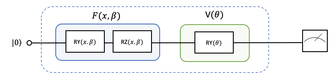
Figure 4: This figure shows a quantum circuit of one qubit with only one repetition (Layer). This circuit implements a trigonometric interpolation (Fourier series), where the repeat frequency of the feature map, thus of the data, defines the angular frequency of the Fourier series: $\sum_{\omega}c_{\omega}e^{i\omega x}$. Our Feature Map, which implements our data encoding strategy, determines the frequencies $\omega$, and our variational quantum circuit determines the coefficients $c_{\omega}$. In blue, the function that implements the feature map, with $\beta$, the scaling hyperparameter, with $x$ the input data. Said data is encoded in the $RY$ and $RZ$ parameterized gates. In green is the variational circuit that forms the proposed parameterized function, with $\theta$, the parameter, one parameter per qubit. Without repeating the layer and reloading the data $x$, this circuit will only learn a $sine$ or $cosine$ function.

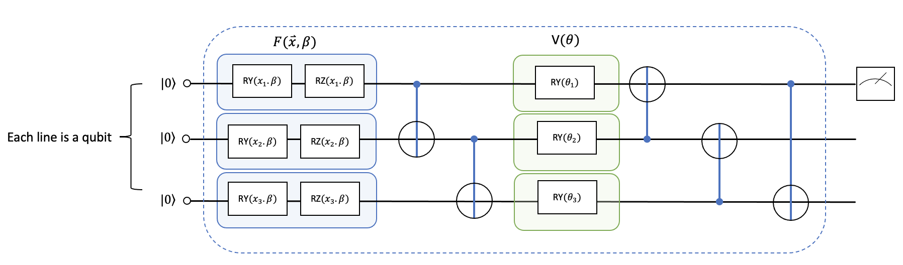
Figure 5: This figure shows a quantum circuit of three qubits with only one repetition (Layer). This circuit implements a trigonometric interpolation (Fourier series), where the repeat frequency of the feature map, thus of the data, defines the angular frequency of the Fourier series: $\sum_{\omega}c_{\omega}e^{i\omega x}$. Our Feature Map, which implements our data encoding strategy, determines the frequencies $\omega$, and our variational quantum circuit determines the coefficients $c_{\omega}$. Each qubit represents a variable of our multivariable function. In blue, the function that implements the feature map, with $\beta$, the scaling hyperparameter, with $x$ the input data. Said data is encoded in the $RY$ and $RZ$ parameterized gates. In green is the variational circuit that forms the proposed parameterized function, with $\theta$, our parameter, one parameter per qubit. We have three. The $CNOT$ gates help us to interleave the data so that we can only read in the first qubit. This allows us to reduce the effect of the barren plateau in the case of a classifier.

Let $\ket{\psi(\vec{x})}$ be a functional quantum state and let $f_{\theta_{i}}(x):\mathbb{R}^{m}\rightarrow\mathbb{C}$ be complex function. Then,

$$\ket{\psi(\vec{x})}=\sum_{i=0}^{2^{n}-1}f_{\theta_{i}}(\vec{x})\ket{i},$$ (28)

$$\sum_{i=0}^{2^{n}-1}|f_{\theta_{i}}(\vec{x})|^{2}=1.$$ (29)

The circuit $\mathcal{U}(\vec{x},\vec{\theta},\beta)$ approximates the state as

$$\ket{\psi(\vec{x})}\sim\mathcal{U}(\vec{x},\vec{\theta},\beta)\ket{0}^{\otimes n},$$ (30)

with

$$\mathcal{U}(\vec{x},\vec{\theta},\beta)=\prod_{i=1}^{k}U(\vec{x}\cdot\beta,\vec{\theta_{i}}),$$ (31)

with better results as the number of layers, repetition $k$ increases, and $n$ the number of classes. $\vec{\theta}=\{\vec{\theta_{i}}\}$ is found with classical optimization techniques. Our Cost function (CF) is calculated by ${\rm distance}(\ket{\psi(\vec{x})},\mathcal{U}(\vec{x},\beta,\vec{\theta})\ket{0}^{\otimes n}).$

With all the last defined, the prediction of the quantum model for each $x$ can be defined as the expectation value of the observable $\sigma_{z}$ concerning the state $\ket{\psi(\vec{x})}$ via our parametrized quantum circuit as follows:

$$f_{\bm{\theta}}(x)=\bra{0}\mathcal{U}^{\dagger}(\vec{x},\vec{\theta},\beta)O\mathcal{U}(\vec{x},\vec{\theta},\beta)\ket{0},$$ (32)

where $O$ is observable that can be one of the Pauli matrices $(I,X,Y,Z)$.

In the case of the binary classifier given by the figure (4), we measure the expected value of the proposed quantum circuit, and after the measurement, we make the sign of the output.

There are two possible scenarios for the multiclass classifier given by figure (5). First, generalize the binary classifier, or second, where we work with the probabilities so that, knowing the highest probability, the class will be known. Although the problem requires much more qubits due to the input data size, in this case, we use gates like $CNOT$, $CRY$, etc., to entangle the qubits and only read, for example, at qubit 0. Although the number of classes grows logarithmically, the effect of the Barren Plateaus Holmes et al. (2022); McClean et al. (2018) is less.

VII Results

Considering the proposed scenarios, this session will present the results obtained during our experimentation.

VII.0.1 TRIGONOMETRIC INTERPOLATION

This subsection presents the experiments’ results using our trigonometric interpolation model. To test it, we operate as the input signal, the function sine, cosine, log, saw-tooth, and square. Figures (6) to (8) show the results from the trigonometric interpolation experiments. We define sample rate frequency to accomplish a Nyquist theorem Landau (1967). Next, we present the results. We have taken the opportunity to study the Gibbs phenomenon in the square and saw-tooth signals.

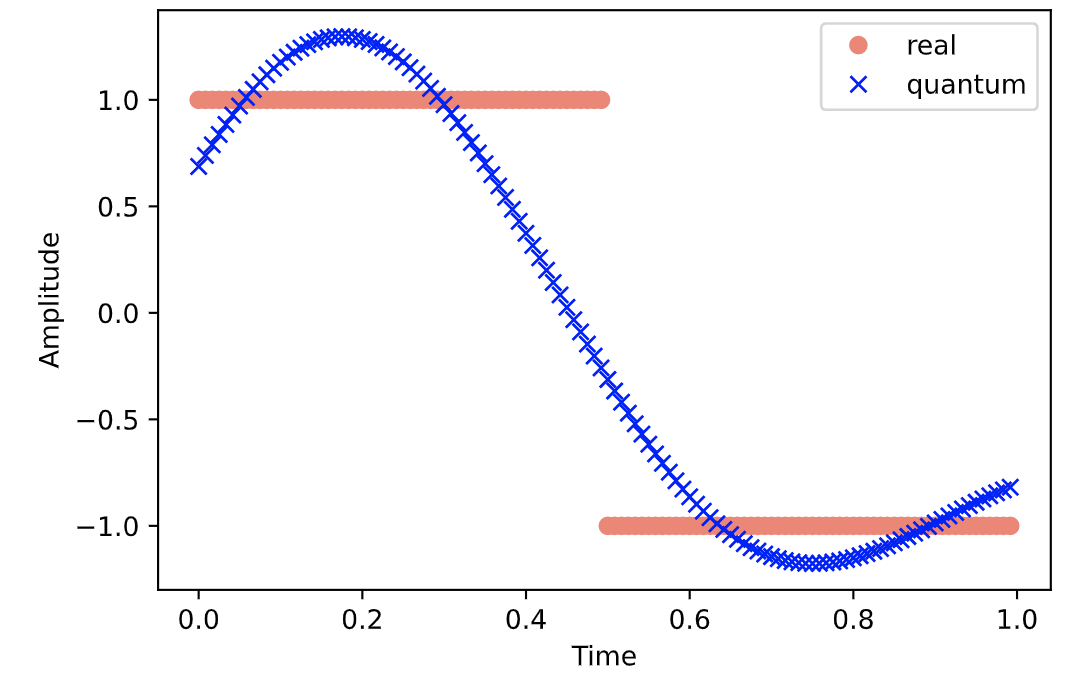
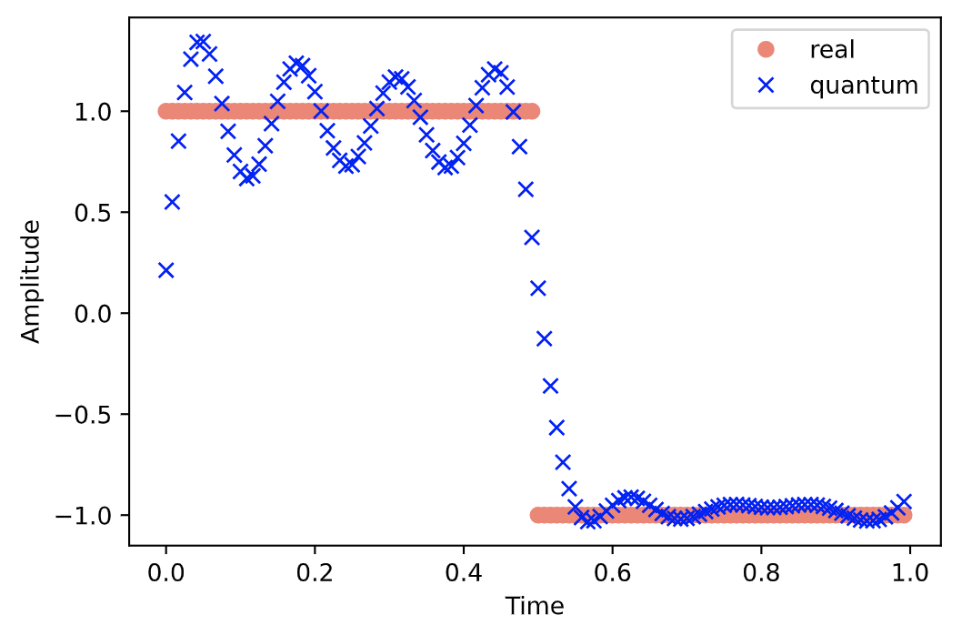
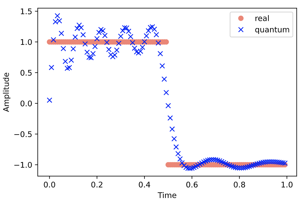
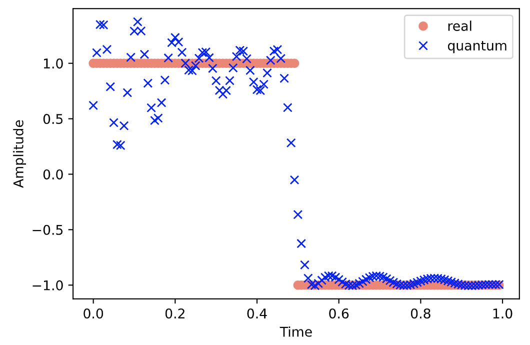
Figure 6: These graphs show the experiment of four tests with the square signal of $20Hz$ with the different number of layers ($L$) and sample ($n$) where the behavior of the trigonometric model on the given input and the decomposition of harmonic frequencies and the Gibbs phenomenon can be observed. With more high-frequency components, the reconstruction of the squared signal is achieved. In the first image on the top left, we observe the effect of the Fourier series approximation with a lower-order polynomial. In this case, with the number of the layers $L=3$ and the number of the sample $n=20$. The second image above to the right is the same scenario as the previous one but with $n=100$. In the third image from the bottom left, we can observe the same input signal of $20Hz$, this time with $L=20$ and the number of points $n=100$. The fourth image from the bottom right shows the same $20Hz$ input signal, with $L=30$ and $n=100$. In all these cases, we have a scaling parameter $\beta$ to better interpolate with high-frequency harmonics.

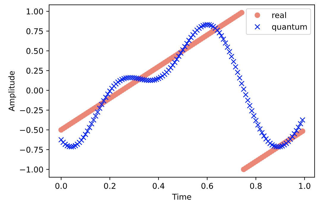
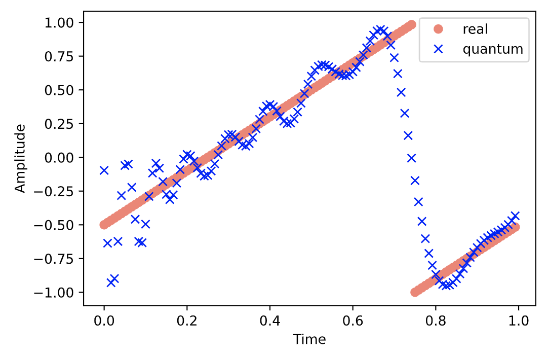
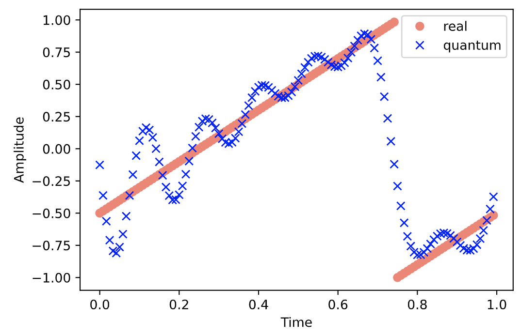
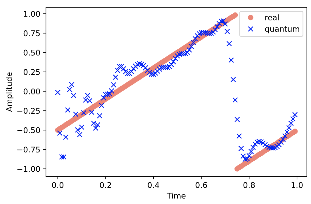
Figure 7: These graphs show the experiment of four tests with the sawtooth signal of $20Hz$ with the different number of layers ($L$) and sample ($n$) where the behavior of the trigonometric model on the given input and the decomposition of harmonic frequencies and the Gibbs phenomenon can be observed. With more high-frequency components, the reconstruction of the squared signal is achieved. In the first image on the top left, we observe the effect of the Fourier series approximation with a lower-order polynomial. In this case, with the number of the layers $L=3$ and the number of the sample $n=20$. The second image above to the right is the same scenario as the previous one but with $n=100$. In the third image from the bottom left, we can observe the same input signal of $20Hz$, this time with $L=20$ and the number of points $n=100$. The fourth image from the bottom right shows the same $20Hz$ input signal, with $L=30$ and $n=100$. In all these cases, we have a scaling parameter $\beta$ to better interpolate with high-frequency harmonics.

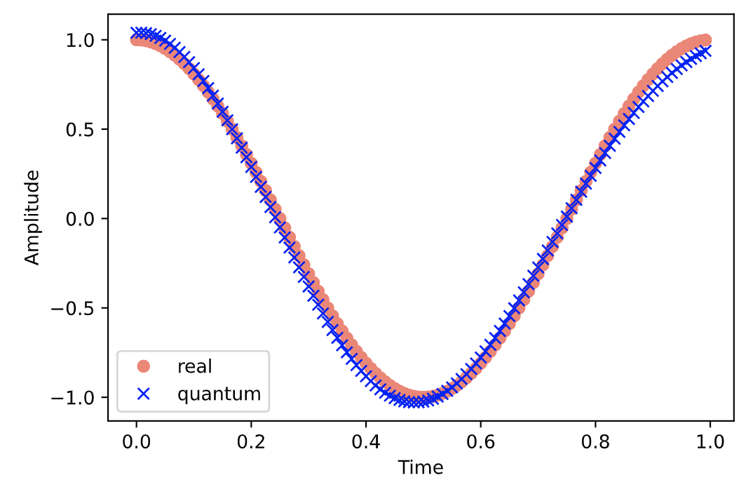
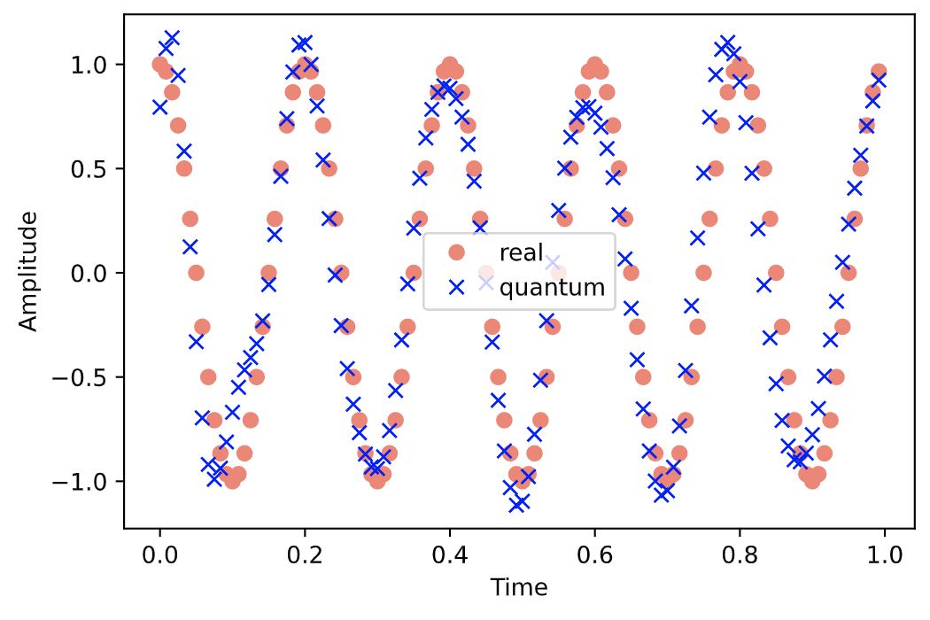
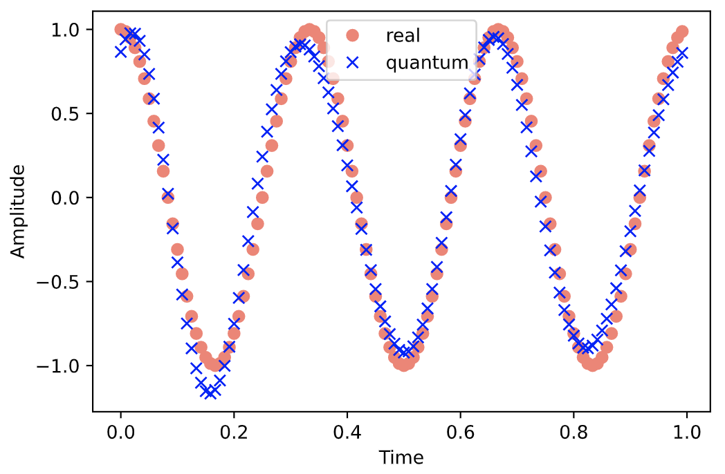
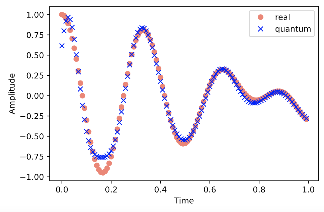
Figure 8: These figures show how the quantum model fits the input of the sine and cosine input signal. Several different frequencies have been tested; amplitude modulations have been tested to analyze how the model follows it. We realized the model limitation on the highest-frequency input signal.

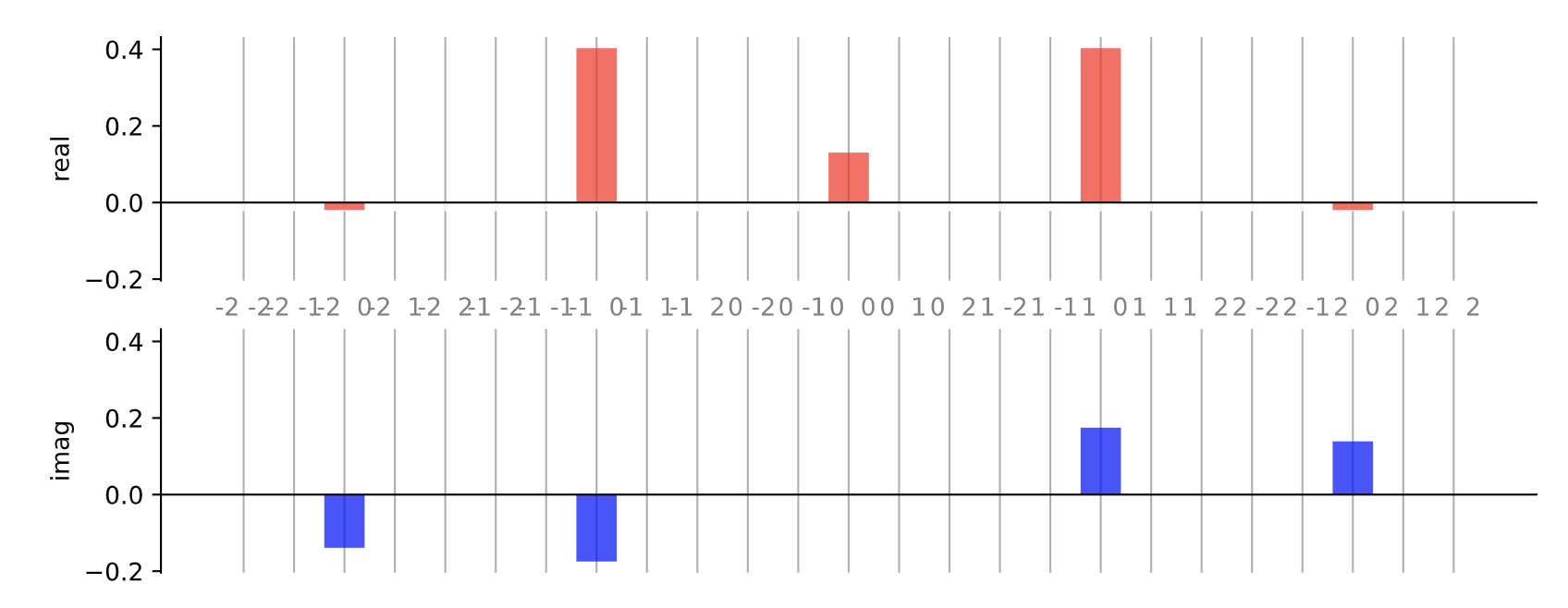
Figure 9: This graph illustrates the Fourier coefficients in the case of a $3Hz$ sinusoidal input signal, sampled above the Nyquist frequency at $120Hz$, and with $12$ repetitions, we can observe that the Fourier coefficients are potentially, in this case, rather real than imagined. Taking advantage of the Pennylane Pennylane (2023) tool, we validate our model provided by figure (10)

.

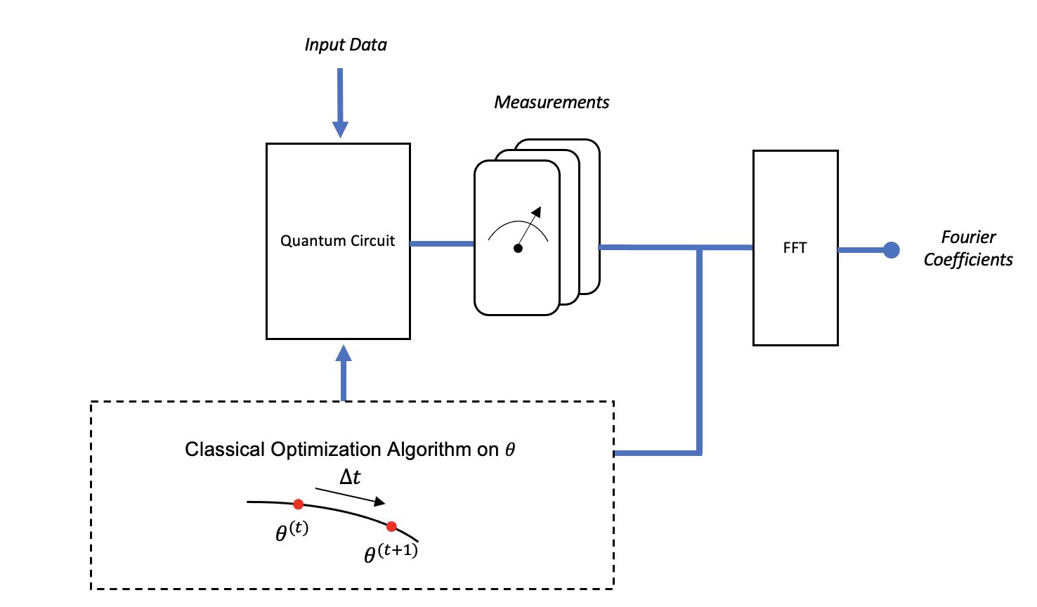
Figure 10: This diagram illustrates the steps to find the Fourier series coefficients using a variational model. The FFT block samples the Fourier coefficients computing the first $2*K+1$ one of a $2*\pi$ periodic input signal, where $K\in N$.

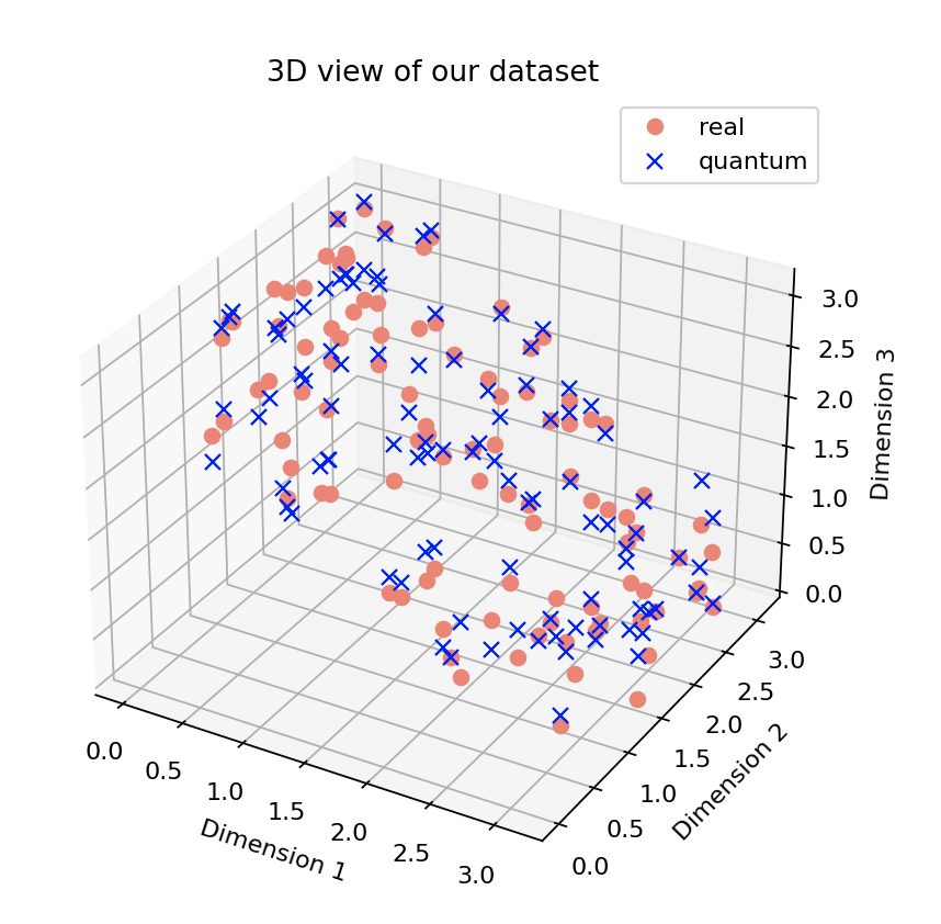
Figure 11: In this graph, we can analyze how we apply our model to data. We can observe how the model allows us to interpolate the data from the dataset better. One possible application is to find a continuous parameterized function from the discrete data. This approach can solve several real problems based on extensive classical data.

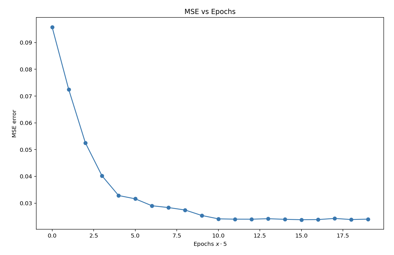
Figure 12: In this graph, we can see the evolution of our cost function. In this case, the equation described in (5).

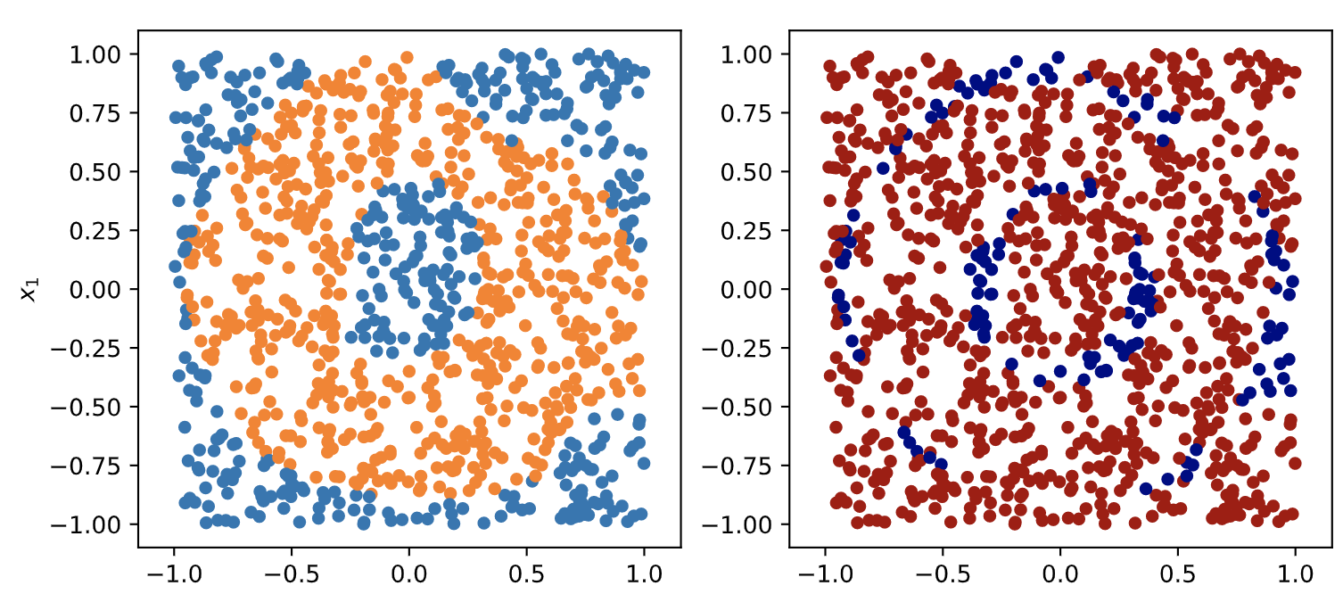
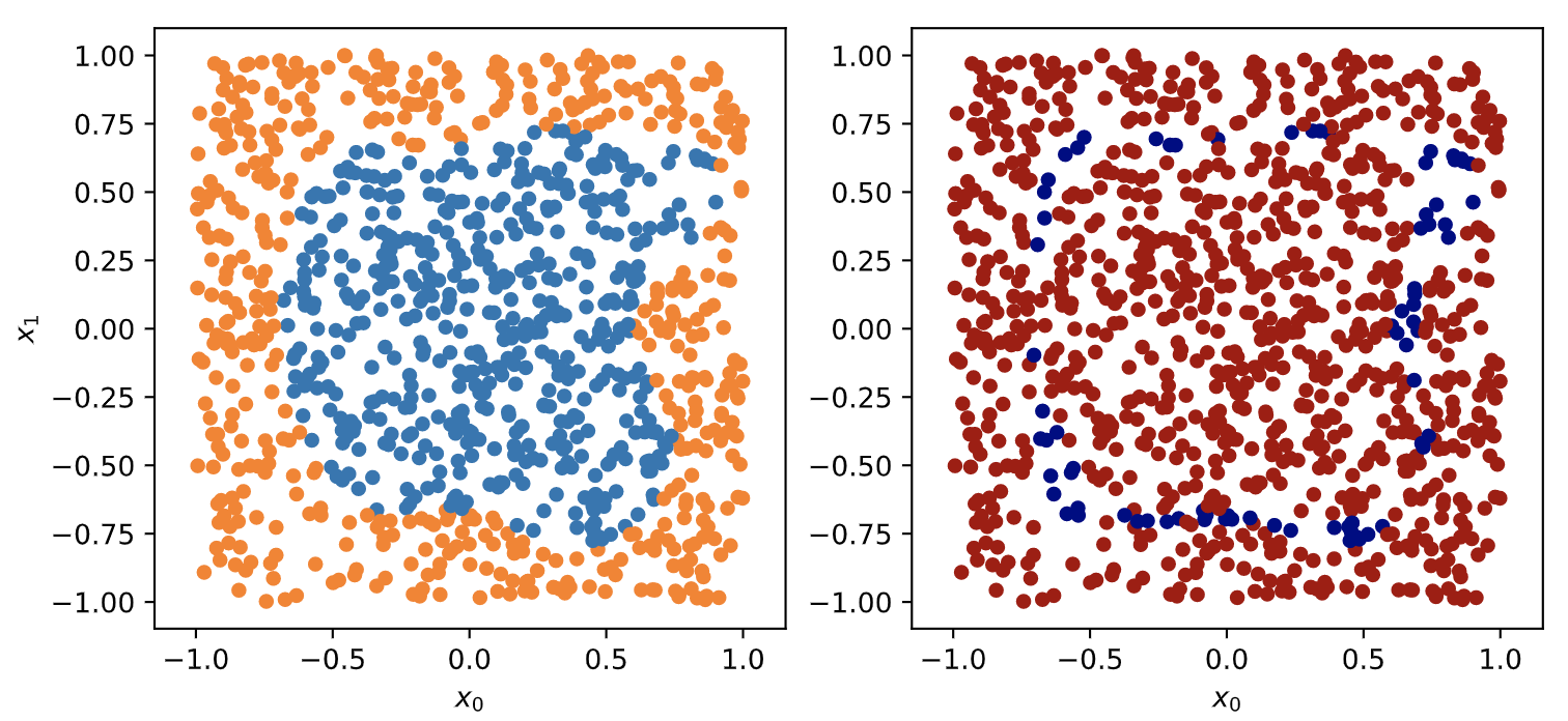
Figure 13: These figures are parts of the experiments we did in the case of the model as a classifier. In the first two graphs, we can observe that the figures above represent two circles. The one on the left is the classifier’s result, and on the right are our model’s classification errors. In this case, we are talking about $92.5\%$ accuracy. In the second two graphs, where the figure is to be classified in a square of others, we see the same in this case, an accuracy of $92.2\%$.

VII.0.2 CLASSIFIERS

In this subsection, we present the results of our experiments with our model in the classification section. To test the classifier, we have generated four datasets (crown, circle, square, SWP Atchade-Adelomou (2022); Atchade Adelomou et al. (2020); Adelomou et al. (2020)). Figures, (12), (13) and table (1) to (3) present the results of the experiments.

Quantum neural classifier ($1$ qubit)
#Layers	#Parameters	Accuracy
1	3	52.60
2	6	59.90
3	9	62.60
4	12	66.61
5	15	63.72
6	18	68.85
7	21	67.91
8	24	67.20
10	30	73.91

Table 1: We can observe from the table and from the outcomes that the proposed model can be used to perform a classifier. This is the table from studying the binary classifier with two qubits. In this study, we consider the circuit depth ($l$), the number of the qubits $n$, and the number of the parameterized gates $m$, the number of parameters calculated as $n\times$m$\times l$. Where $m$ is the summation of the parameterized gates of the feature map stage and the variational quantum algorithm.

Quantum neural classifier ($2$ qubits)
#Layers	#Parameters	Accuracy
1	6	48.90
2	12	70.30
3	18	84.5
4	24	84.90
5	30	87.50
6	36	92.10
7	42	92.60
8	48	92.50
10	60	92.20

Table 2: We can observe from the table and from the outcomes that the proposed model can be used to perform a classifier. This is the table from studying the binary classifier with two qubits. In this study, we consider the circuit depth ($l$), the number of the qubits $n$, and the number of the parameterized gates $m$, the number of parameters calculated as $n\times$m$\times l$ where $m$ is the summation of the parameterized gates of the feature map stage and the variational quantum algorithm.

The SWP leveraged the quantum neural classifier.
#Patients	#SW	#Layers	Accuracy
3	2	2	70.3
4	3	2	63.2
5	2	2	57.7
5	3	2	48.1
5	4	2	47.2

Table 3: We are solving the Social Workers’ Problem (SWP) Atchade-Adelomou (2022); Atchade Adelomou et al. (2020); Adelomou et al. (2020) with a quantum neural network classifier.

VII.1 Discussions

Future work will apply the ideas developed here in a real model. Although intuition leads us to think that the quantum model is a Fourier series, basically because the parameterized gates define the ansatz are rotation gates, the demonstration of this intuition is not trivial. Calculating the Fourier coefficients of the quantum model is also very challenging. In this paper, we have relied on an approximation and classical with the fft to calculate them (see figure (10)). We have confirmed that the proposed model is a partial Fourier series. The model can be used for trigonometric interpolation (see Figures (6) to (11)), as seen in the figure (11), Also, with a few subtle changes, we have been able to make a binary classifier (see figure (12) to (13)). It is worth determining the sign for a binary classifier to know what class it is in. We can perform it with expectation value (qml.expval) or with probabilities (qml.probs). In the case of having a multiclass classifier, what can be done is to generalize the binary classifier or work with the probabilities so that, knowing the highest probability of the measured outcome, the class will be known. Nevertheless, it is costly to go from binary classifier to multiclass; one must run $(n+1)n/2$ quantum models.

We have not made a detailed study of the algorithm’s computational complexity; however, in case of a volume of data that presents a trigonometric distribution, the proposed model will be able to speed up the hyperparameter optimization process. This model can help to find hyperparameters more optimally and can help to have a continuous function model from discrete function models, thus offering more valuable solutions.

Tables (1) and (2) give us detailed information on the quality of the classifier that we have managed to have some classifiers with accuracy greater than 92%. From figure (14), which represents the amplitude modulation, we can analyze the limitation of the proposed model for the highest frequencies where we can observe how the tail of the signal is seen to decay, and during the experimentation, we decided to increase the number of repetitions (layers) to adapt the model to the input signal.

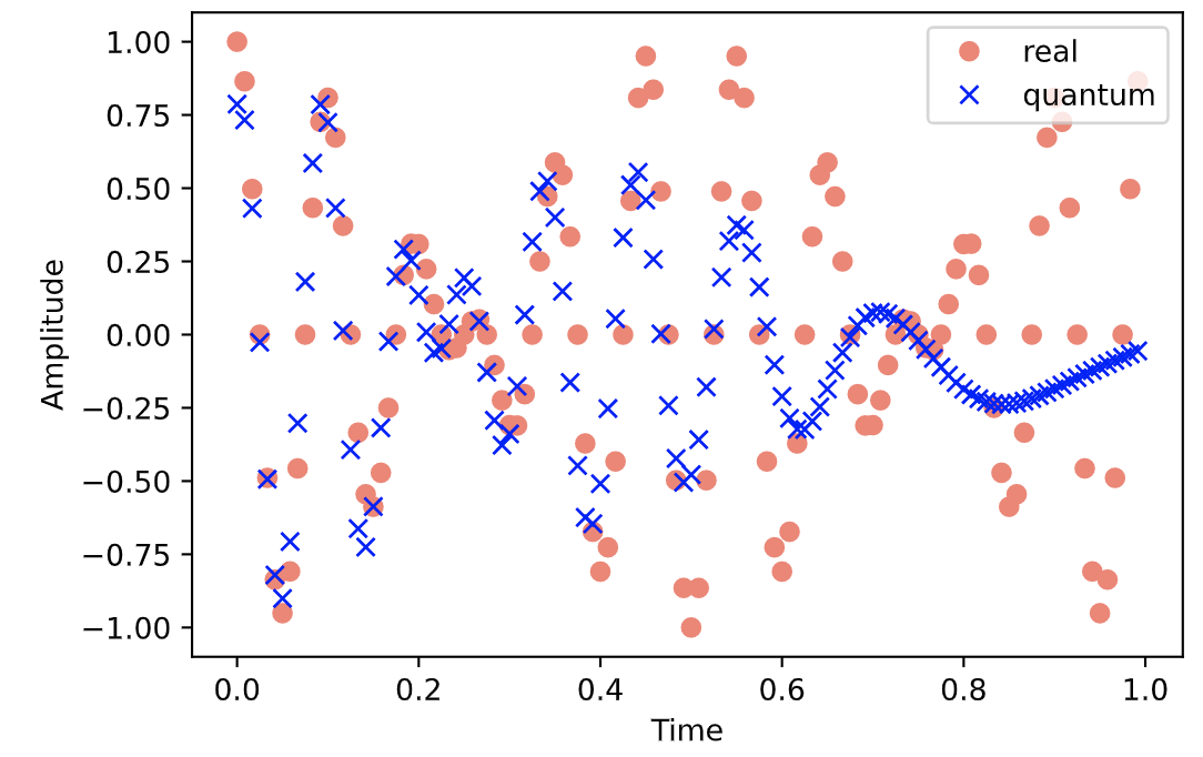
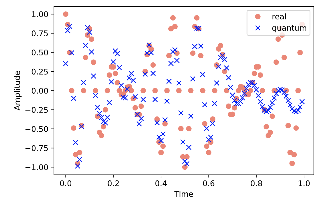
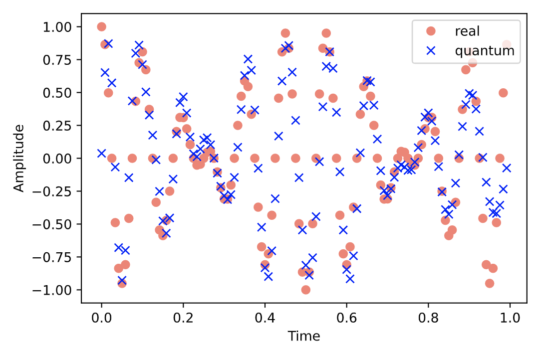
Figure 14: This graph presents the behavior experiment due to the limitations of high frequencies. The tail of the signal is seen to decay, and we must considerably increase the number of repetitions (layers) to solve it. In this graph, we multiply two quite different frequency sines. This is the result of simulating an amplitude modulation.

VIII Conclusion

In this paper, we have experimented with and demonstrated the weight of the Fourier series in quantum machine learning. It also analyzed its impact on interpolations that can be used for banking problems, airline companies, retail companies, hyperparameter searches problems, etc. We have also analyzed its impact on binary and multiclass classifiers, Hamiltonian simulation, and signal processing applications. The results conclude that we can strongly consider the quantum computer a Fourier series. However, we have also detected some limitations in better adapting the model to the highest-frequency input signals. Also, it remains a challenge to finish determining with greater precision the Fourier coefficients. The way we have found to determine the Fourier coefficients from the VQA model is given in figure (10). As a line for the future, we want to apply this model to the real problems in the banking sector, mobility, etc.

Code

The reader can find the code in the following GitHub repository: https://github.com/pifparfait/Fourier_Based_QML to reproduce the figures and explore different settings of the proposed model.

References

- Chaudhuri and Feireisl (2022) Nilasis Chaudhuri and Eduard Feireisl, “Navier–stokes–fourier system with dirichlet boundary conditions,” Applicable Analysis 101, 4076–4094 (2022).
- Ambainis (2007) Andris Ambainis, “Quantum walk algorithm for element distinctness,” SIAM Journal on Computing 37, 210–239 (2007).
- Schuld and Petruccione (2018) Maria Schuld and Francesco Petruccione, Supervised learning with quantum computers, Vol. 17 (Springer, 2018).
- Kempe et al. (2006) Julia Kempe, Alexei Kitaev, and Oded Regev, “The complexity of the local hamiltonian problem,” Siam journal on computing 35, 1070–1097 (2006).
- Childs and Kothari (2010) Andrew M Childs and Robin Kothari, “Simulating sparse hamiltonians with star decompositions,” in Conference on Quantum Computation, Communication, and Cryptography (Springer, 2010) pp. 94–103.
- Hatano and Suzuki (2005) Naomichi Hatano and Masuo Suzuki, “Finding exponential product formulas of higher orders,” in Quantum annealing and other optimization methods (Springer, 2005) pp. 37–68.
- Meister et al. (2022) Richard Meister, Simon C Benjamin, and Earl T Campbell, “Tailoring term truncations for electronic structure calculations using a linear combination of unitaries,” Quantum 6, 637 (2022).
- Wang et al. (2021) Shengbin Wang, Zhimin Wang, Guolong Cui, Shangshang Shi, Ruimin Shang, Lixin Fan, Wendong Li, Zhiqiang Wei, and Yongjian Gu, “Fast black-box quantum state preparation based on linear combination of unitaries,” Quantum Information Processing 20, 1–14 (2021).
- Alonso-Linaje and Atchade-Adelomou (2021) Guillermo Alonso-Linaje and Parfait Atchade-Adelomou, “Eva: a quantum exponential value approximation algorithm,” (2021).
- De Raedt and De Raedt (1983) Hans De Raedt and Bart De Raedt, “Applications of the generalized trotter formula,” Physical Review A 28, 3575 (1983).
- Guerreschi (2019) Gian Giacomo Guerreschi, “Repeat-until-success circuits with fixed-point oblivious amplitude amplification,” Physical Review A 99, 022306 (2019).
- Novo and Berry (2016) Leonardo Novo and Dominic W. Berry, “Improved hamiltonian simulation via a truncated taylor series and corrections,” (2016), 10.48550/ARXIV.1611.10033.
- Eldar and Oppenheim (2002) Yonina C Eldar and Alan V Oppenheim, “Quantum signal processing,” IEEE Signal Processing Magazine 19, 12–32 (2002).
- Silva et al. (2022) Thais de Lima Silva, Lucas Borges, and Leandro Aolita, “Fourier-based quantum signal processing,” (2022).
- Du et al. (2020) Yuxuan Du, Min-Hsiu Hsieh, Tongliang Liu, and Dacheng Tao, “Expressive power of parametrized quantum circuits,” Physical Review Research 2, 033125 (2020).
- Schuld et al. (2021) Maria Schuld, Ryan Sweke, and Johannes Jakob Meyer, “Effect of data encoding on the expressive power of variational quantum-machine-learning models,” Physical Review A 103 (2021), 10.1103/physreva.103.032430.
- Pérez-Salinas et al. (2020) Adrián Pérez-Salinas, Alba Cervera-Lierta, Elies Gil-Fuster, and José I Latorre, “Data re-uploading for a universal quantum classifier,” Quantum 4, 226 (2020).
- Killoran et al. (2019) Nathan Killoran, Thomas R Bromley, Juan Miguel Arrazola, Maria Schuld, Nicolás Quesada, and Seth Lloyd, “Continuous-variable quantum neural networks,” Physical Review Research 1, 033063 (2019).
- Sim et al. (2019) Sukin Sim, Peter D Johnson, and Alán Aspuru-Guzik, “Expressibility and entangling capability of parameterized quantum circuits for hybrid quantum-classical algorithms,” Advanced Quantum Technologies 2, 1900070 (2019).
- Chen et al. (2021) Hongxiang Chen, Leonard Wossnig, Simone Severini, Hartmut Neven, and Masoud Mohseni, “Universal discriminative quantum neural networks,” Quantum Machine Intelligence 3, 1–11 (2021).
- Biamonte (2021) Jacob Biamonte, “Universal variational quantum computation,” Physical Review A 103, L030401 (2021).
- Schuld et al. (2015) Maria Schuld, Ilya Sinayskiy, and Francesco Petruccione, “An introduction to quantum machine learning,” Contemporary Physics 56, 172–185 (2015).
- Biamonte et al. (2017) Jacob Biamonte, Peter Wittek, Nicola Pancotti, Patrick Rebentrost, Nathan Wiebe, and Seth Lloyd, “Quantum machine learning,” Nature 549, 195–202 (2017).
- Dunjko et al. (2016) Vedran Dunjko, Jacob M Taylor, and Hans J Briegel, “Quantum-enhanced machine learning,” Physical review letters 117, 130501 (2016).
- Atchade Adelomou et al. (2020) Parfait Atchade Adelomou, Elisabet Golobardes Ribé, and Xavier Vilasís Cardona, “Using the variational-quantum-eigensolver (vqe) to create an intelligent social workers schedule problem solver,” in International Conference on Hybrid Artificial Intelligence Systems (Springer, 2020) pp. 245–260.
- Atchade-Adelomou and Alonso-Linaje (2022) Parfait Atchade-Adelomou and Guillermo Alonso-Linaje, “Quantum-enhanced filter: Qfilter,” Soft Computing , 1–8 (2022).
- Adelomou et al. (2022) Parfait Atchade Adelomou, Daniel Casado Fauli, Elisabet Golobardes Ribé, and Xavier Vilasis-Cardona, “Quantum case-based reasoning (qcbr),” Artificial Intelligence Review , 1–27 (2022).
- Guillermo (2023) Alonso-Linaje Guillermo, “¿quieres aprender computación cuántica ?” (2023).
- Havlíček et al. (2019) Vojtěch Havlíček, Antonio D Córcoles, Kristan Temme, Aram W Harrow, Abhinav Kandala, Jerry M Chow, and Jay M Gambetta, “Supervised learning with quantum-enhanced feature spaces,” Nature 567, 209–212 (2019).
- Schuld and Killoran (2019) Maria Schuld and Nathan Killoran, “Quantum machine learning in feature hilbert spaces,” Physical review letters 122, 040504 (2019).
- Wittek and Cucchietti (2013) Peter Wittek and Fernando M Cucchietti, “A second-order distributed trotter–suzuki solver with a hybrid cpu–gpu kernel,” Computer Physics Communications 184, 1165–1171 (2013).
- Lloyd et al. (2020) Seth Lloyd, Maria Schuld, Aroosa Ijaz, Josh Izaac, and Nathan Killoran, “Quantum embeddings for machine learning,” arXiv preprint arXiv:2001.03622 (2020).
- Suzuki et al. (2020) Yudai Suzuki, Hiroshi Yano, Qi Gao, Shumpei Uno, Tomoki Tanaka, Manato Akiyama, and Naoki Yamamoto, “Analysis and synthesis of feature map for kernel-based quantum classifier,” Quantum Machine Intelligence 2, 1–9 (2020).
- Gil Vidal and Theis (2020) Francisco Javier Gil Vidal and Dirk Oliver Theis, “Input redundancy for parameterized quantum circuits,” Frontiers in Physics 8, 297 (2020).
- SAKURAI (1938) Tokio SAKURAI, “An extension of parseval theorem,” Proceedings of the Physico-Mathematical Society of Japan. 3rd Series 20, 162–165 (1938).
- Holmes et al. (2022) Zoë Holmes, Kunal Sharma, Marco Cerezo, and Patrick J Coles, “Connecting ansatz expressibility to gradient magnitudes and barren plateaus,” PRX Quantum 3, 010313 (2022).
- McClean et al. (2018) Jarrod R McClean, Sergio Boixo, Vadim N Smelyanskiy, Ryan Babbush, and Hartmut Neven, “Barren plateaus in quantum neural network training landscapes,” Nature communications 9, 1–6 (2018).
- Landau (1967) HJ Landau, “Sampling, data transmission, and the nyquist rate,” Proceedings of the IEEE 55, 1701–1706 (1967).
- Pennylane (2023) Xanadu Pennylane, “This module contains functions to analyze the fourier representation of quantum circuits.” (2023).
- Atchade-Adelomou (2022) Parfait Atchade-Adelomou, “Quantum algorithms for solving hard constrained optimisation problems,” (2022).
- Adelomou et al. (2020) Atchade Parfait Adelomou, Elisabet Golobardes Ribé, and Xavier Vilasis Cardona, “Formulation of the social workers’ problem in quadratic unconstrained binary optimization form and solve it on a quantum computer,” Journal of Computer and Communications 8, 44–68 (2020).