Deep Active Learning for Scientific Computing in the Wild

Abstract

Deep learning (DL) is revolutionizing the scientific computing community. To reduce the data gap caused by usually expensive simulations or experimentation, active learning has been identified as a promising solution for the scientific computing community. However, the deep active learning (DAL) literature is currently dominated by image classification problems and pool-based methods, which are not directly transferrable to scientific computing problems, dominated by regression problems with no pre-defined ’pool’ of unlabeled data. Here for the first time, we investigate the robustness of DAL methods for scientific computing problems using ten state-of-the-art DAL methods and eight benchmark problems. We show that, to our surprise, the majority of the DAL methods are not robust even compared to random sampling when the ideal pool size is unknown. We further analyze the effectiveness and robustness of DAL methods and suggest that diversity is necessary for a robust DAL for scientific computing problems.

Keywords Deep Learning  $\cdot$ Active Learning  $\cdot$ Regression  $\cdot$ Query-by-committee  $\cdot$ Query Synthesis  $\cdot$ Inverse Problem  $\cdot$ Scientific Computing  $\cdot$ Artificial Electromagnetic Material

1 Introduction

Deep learning - primarily deep neural networks (DNNs) - has led to major breakthroughs in scientific computing in recent years [1, 2, 3, 4], such as chemistry [5], materials science [6], and biology [7]. Given its significance, it has emerged in recent years as a major area of research in the machine learning community [3], involving a variety of unique technical challenges. One such challenge - shared by many disciplines - is that DNNs require significant quantities of training data [8]. One widely-studied strategy to mitigate this problem is active learning (AL)[9, 10], and we focus here on active learning specifically for DNNs, sometimes referred to as Deep Active Learning (DAL) [11].

Broadly speaking, the premise of DAL is that some training instances will lead to greater model performance than others. Therefore we can improve the training sample efficiency of DNNs by selecting the best training instances. A large number methods have been investigated in recent years for DAL [10, 9], often reporting significant improvements in sample efficiency compared to simpler strategies, such as random sampling [12, 13, 14]. While these studies are encouraging and insightful, they nearly always assume that one or more DAL hyperparmeters are known prior to deployment (i.e., collection of labeled data). While such assumptions are realistic in many contexts of machine learning, the hyperparameters of many DAL require labeled data (see Section 3) to be optimized which, by assumption, are not yet available. It is therefore unclear how these hyperparameters should be set when DAL is applied to new problems, and whether DAL still offers advantages over alternative methods when accounting for hyperparameter uncertainty. Although rarely discussed in the literature, this is a problem users face when applying DAL in to new problems in real-world conditions, or "in the wild" as it is sometimes described [15].

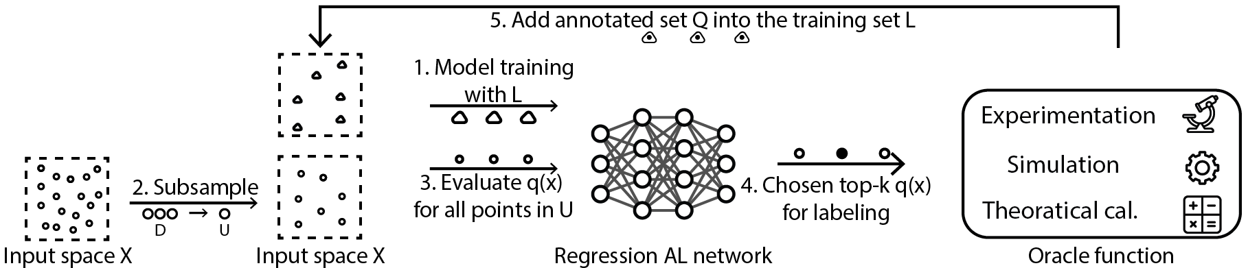
This problem is especially acute in scientific computing applications because nearly all applicable DAL methods are pool-based, illustrated in Fig 1. Scientific computing most often utilizes DNNs for regression tasks, where nearly all applicable DAL methods are pool-based; these methods rely upon selecting unlabeled points (i.e., settings of $x$) to label from a finite pre-existing set, or "pool". This is in contrast to query synthesis methods, for example, which consider all possible settings of $x$ (e.g., all possible settings of $N$-dimensional real numbers). As we argue in this work (see Section 3), all pool-based methods share a common hyperparameter, termed the pool ratio, $\gamma$, which cannot be optimized without significant quantities of labeled data, and which (as we show) has a significant impact on the effectiveness of DAL methods.

Figure 1: Schematic diagram for pool-based deep active learning procedure for scientific computing. In the input space X, the triangles represent labeled data ($L$), and the circles represent unlabeled data ($D$ for the full set of possibly infinite unlabeled $x$, $U$ for current unlabeled pool). At each step, after the model is trained using the existing training set $L$, a subset of unlabeled data $U$ is sampled and evaluated by the AL criteria q(x). Then the top-k points according to q(x) are then labeled by the oracle function.

1.1 Contributions of this work

In this work we investigate the effectiveness of DAL methods in scientific computing applications, in the wild. Specifically, we investigate DAL performance when the optimal setting of $\gamma$ is not known in advance. Although many DAL methods have additional hyperaparameters that cannot be optimized apriori, we focus on $\gamma$ because it is shared by nearly all DAL methods that are applicable to scientific computing (i.e., regression problems). To support our investigation, we assembled eight scientific computing problems to examine the performance of DAL methods in this setting; to our knowledge, this is the first such benchmark of its kind. We then identified past and recent DAL methods that are suitable for scientific computing problems (i.e., regression), totaling ten methods. Our collection of benchmark methods encompasses many DAL methods that are employed beyond scientific computing, making our findings relevant to the broader active learning community as well.

We examine the performance of our DAL methods on each of our eight benchmark problems, compared to simple random sampling, and also as we vary their $\gamma$ setting. Our results indicate that their performance varies significantly with respect to $\gamma$ within our range, and that no single $\gamma$ setting works well across all problems. To characterize the real-world performance of the DAL models, we also examined their performance under three key conditions: (i) when $\gamma$ is set to the optimal value in each problem, (ii) the worst value in each problem, and (iii) when we choose the best overall setting across all eight problems (i.e., each problem gets the same setting of $\gamma$, per method). Although many models often perform worse than random sampling, the results indicate that some methods consistently outperform random sampling, even with a poor $\gamma$ setting. We now summarize our contributions:

• We develop the first large benchmark for DAL in scientific computing (e.g., regression problems), involving ten state-of-the-art DAL methods and eight datasets. We publish the datasets and code to facilitate reproducibility.

• Using our benchmark, we perform the first analysis of DAL performance in the wild. We highlight the rarely-discussed problem that some DAL hyperparameters cannot be known prior to model deployment, such as pool ratio ($\gamma$), and that existing DAL models may be sensitive to them. We investigate the performance of our DAL methods when $\gamma$ is not assumed known, and we find in this setting that many DAL models often perform no better than random sampling. Crucially, we find that some DAL still consistently outperform random sampling.

• We analyze the factors that contribute to robustness of DAL. Our results suggest that simply maximizing diversity of sampled data in $x$-space is the most reliable way to get robustness. This is a surprising finding, suggesting that existing uncertainty based DAL models do not robustly leverage information from the learner - a premise of many AL models.

2 Related works

Active learning benchmarks. The majority of the existing AL benchmarks are for classification tasks, rather than regression, and many AL methods for classification cannot be applied to regression, making them unsuitable for most scientific computing applications. Some existing studies include [16], which benchmarked AL using a Support Vector Machine (SVM) with 17 AL methods on 35 datasets. [17] benchmarked logistic regression with ten AL methods and 44 datasets. [18] benchmarked specific entity matching application (classification) of AL with three AL methods on ten datasets, with three different types of classifiers (DNN, SVM, and Tree-based). [19] benchmarked an AL application in outlier detection on 20 datasets and discussed the limitation of simple metrics extensively. [20] benchmarked five classification tasks (including both image and text) using DNN. [21] benchmarked multiple facets of DAL on five image classification tasks.

For the regression AL benchmark, [22] benchmarked five AL methods and seven UCI datasets, but they only employed linear models. [23] compared five AL methods on 12 UCI regression datasets, also using linear regression models. Our work is fundamentally different with both as we use DNNs as our regressors, and we employ several recently-published scientific computing problems that also involved DNN regressors, making them especially relevant for DAL study.

Active learning for regression problems. As discussed, scientific primarily involves regression problems which has received (relatively) little attention compared to classification [9, 24].

For the limited AL literature dedicated to regression tasks, Expected Model Change (EMC) [25] was explored, where an ensemble of models was used [26] to estimate the true label of a new query point using both linear regression and tree-based regressors. Gaussian processes were also used with a natural variance estimate on unlabeled points in a similar paradigm [13]. [27] used Query By Committee (QBC), which trains multiple networks and finds the most disagreeing unlabeled points of the committee of models trained. [12] used the Monte Carlo drop-out under a Bayesian setting, also aiming for the maximally disagreed points. [28] found $x$-space-only methods outperforming y-space methods in robustness. [29] proposed an uncertainty-based mechanism that learns to predict the loss using an auxiliary model that can be used on regression tasks. [30] and [31] used Expected Model Output Change (EMOC) with Convolutional Neural Network (CNN) on image regression tasks with different assumptions. We’ve included all the above-mentioned methods that used deep learning in our benchmarks.

DAL in the wild. To our knowledge, all empirical studies of pool-based DAL methods assume that an effective pool ratio hyperparameter, $\gamma$, is known apriori. While the majority of the work assumed the original training set as the fixed, unlabeled pool, [29] explicitly mentioned their method work with a subset of 10k instead of the full remaining unlabeled set and [32] also mentioned subsampling to create the pool $U$ (and hence $\gamma$). In real-world settings - termed in the wild - we are not aware of any method to set $\gamma$ apriori, and there has been no study of DAL methods under this setting; therefore, to our knowledge, ours is the first such study.

3 Problem Setting

In this work, we focus on DAL for regression problems, which comprise the majority of scientific computing problems involving DNNs. As discussed in Sec. 1, nearly all DAL methods for regression are pool-based, which is one of the three major paradigms of AL (along with stream-based and query synthesis)[10].

Formal description. Let $L^{i}=(X^{i},Y^{i})$ be the dataset used to train a regression model at the $i^{th}$ iteration of active learning. We assume access to some oracle (e.g., a computational simulator for scientific computing problems), denoted $f:\mathcal{X}\rightarrow\mathcal{Y}$, that can accurately produce the target values, $y\in\mathcal{Y}$ associated with input values $x\in\mathcal{X}$. Since we focus on DAL, we assume a DNN as our regression model, denoted $\hat{f}$. We assume that some relatively small number of $N_{0}$ labeled training instances are available to initially train $\hat{f}$, denoted $L^{0}$. In each iteration of DAL, we must get $k$ query instances $x_{k}\in\mathcal{X}$ to be labeled by the oracle, yielding a set of labeled instances, denoted $Q$, that is added to the training dataset. Our goal is then to choose $L$ that maximizes the performance of the DNN-based regression models over unseen test data at each iteration of active learning.

Pool-based Deep Active Learning. General pool-based DAL methods assume that we have some pool $U$ of $N_{U}$ unlabeled instances from which we can choose the $k$ instances to label. Most pool-based methods rely upon some acquisition function $q:\mathcal{X}\rightarrow\mathbb{R}$ to assign some scalar value to each $x\in U$ indicating its "informativeness", or utility for training $\hat{f}$. In each iteration of active learning, $q$, is used to evaluate all instances in $U$, and the top $k$ are chosen to be labeled and included in $L$. This general algorithm is outlined in Algorithm 1.

Algorithm 1 Generic pool-based active learning algorithm

  Input: Initial labeled training set $L^{0}$ of size $N_{ini}$, step size $k$, AL criteria function $q$, number of steps $I$

  for $i=0$ to $I$ do

     Train DNN-based model(s) using training set $L^{i}$

     Create $U$ by sampling $N_{U}$ instances $x\in\mathcal{X}$

     Calculate $q(x)\;\forall x\in U$

     Create $L$ by labeling top $k$ points in $U$ ranked by $q(x)$

     $L^{i+1}=L^{i}\cup Q$

  end for

Figure 2: Schematic diagram for pool-based DAL for uncertainty-based mechanism. $q(x)$ is the acquisition metric. (a, b) are two scenarios of the pool ratio ($\gamma$) being too small (4 in b) or too large (32 in c) in $k$ (step size) of 2.

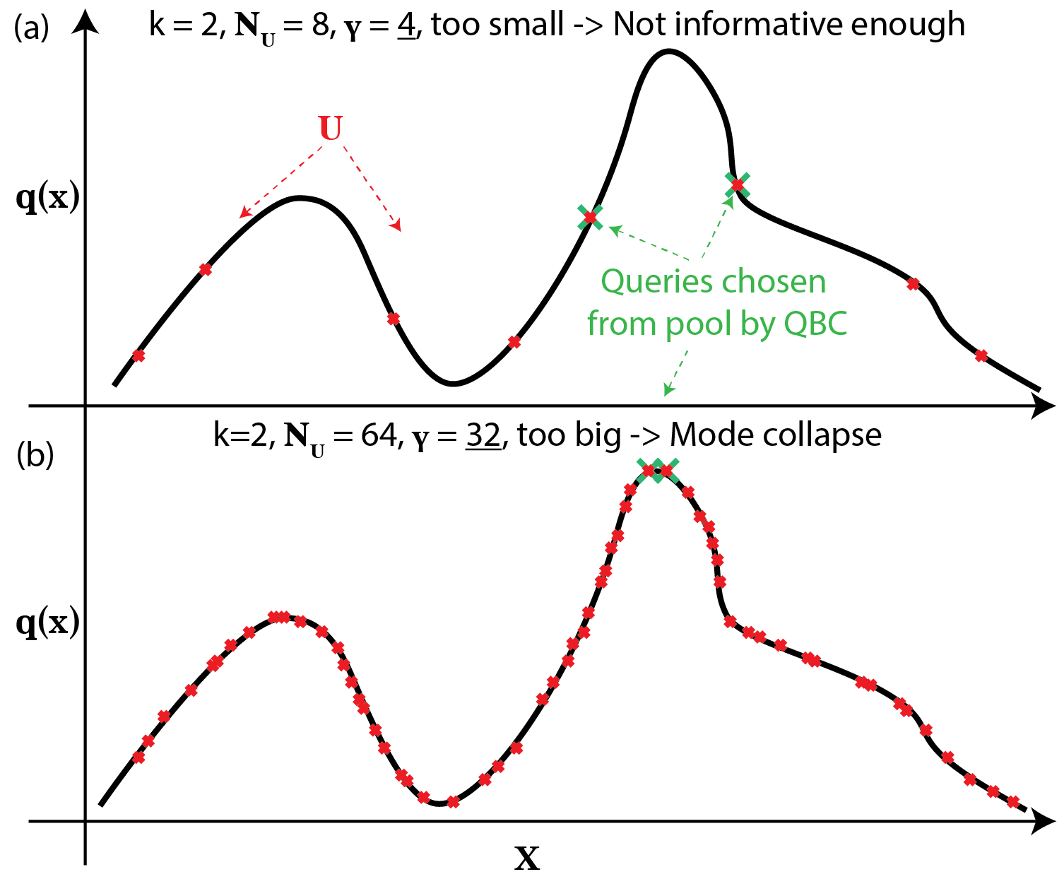
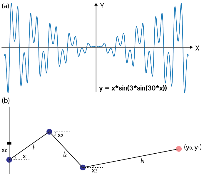
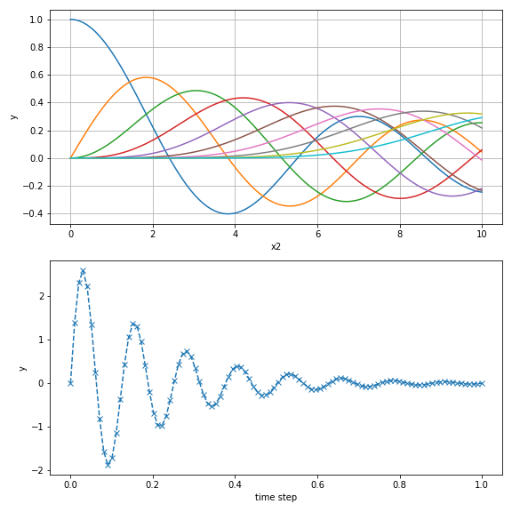
The pool ratio hyperparameter, $\gamma$. We define the pool ratio as $\gamma=N_{U}/k$. By definition, $N_{U}$ and $k$ are hyperparameters of pool-based problems, and therefore $\gamma$ also is. While one could, in principle, vary $N_{U}$ and $k$ independently, this is not often done in practice. Typically $k$ is set as small as possible, limited by computational resources. This leaves $N_{U}$ as the major free hyperparameter, however, prior research has found that its impact depends strongly upon its size relative to $k$ [14, 12, 13], encoded in $\gamma$. Given a fixed value of $k$, a larger value of $N_{U}$ can lead to the discovery of points with larger values of $q(x)$ because the input space is sampled more densely; however, larger $N_{U}$ also tends to increase the similarity of the points, so that they provide the same information to the model - a problem sometimes called mode collapse [33, 9, 14]. In the limit as $N_{U}\rightarrow\infty$ all of the $k$ selected query points will be located near the same $x\in\mathcal{X}$ that has the highest value of $q(x)$. This tradeoff is illustrated in Fig. 2(a-b) for a simple problem.

In most real-world settings, there is a substantial quantity of unlabeled data (often infinite), and the user has the freedom (or burden) of choosing a suitable $\gamma$ setting for their problem by varying the size of $U$. Crucially, and as we show in our experiments, choosing a sub-optimal $\gamma$ value can result in poorer performance than naive random sampling. This isn’t necessarily a problem if either (i) one $\gamma$ setting works across most problems or, alternatively, (ii) $\gamma$ can be optimized on new problems without using labels. To the best of our knowledge, there is no method for optimizing $\gamma$ on a new problem without running multiple trials of AL to find the best one (i.e., collecting labels), defeating the purpose of AL in real-world settings. Furthermore, the value of $\gamma$ varies widely across the literature, suggesting that suitable settings for $\gamma$ indeed vary across problems (see supplement for a list).

4 Benchmark Regression Problems

Table 1: Benchmark datasets dimensionality and oracle functions. $Dim_{x,y}$ are the dimensionality of $x$ and y. Note that ODE solutions are implemented in the form of analytical functions as well.

Data	$Dim_{x}$	$Dim_{y}$	(Proxy) Oracle
Sine	1	1	Analytical
Robo	4	2	Analytical
Stack	5	201	Numerical simulator
ADM	14	2000	Neural simulator
Foil	5	1	Random Forest
Hydr	6	1	Random Forest
Bess	2	1	ODE solution
Damp	3	100	ODE solution

We propose eight regression problems to include in our public DAL regression benchmark: two simple toy problems (SINE, ROBO), four contemporary problems from recent publications in diverse fields of science and engineering (STACK, ADM, FOIL, HYDR) and two problems solving ordinary differential equations (also prevalent in engineering). Scientific computing problems vary substantially in their dimensionality (see [3, 34, 35] for varying examples). We chose relatively lower-dimensional problems because they are still common in the literature, while facilitating larger-scale experimentation and reproducibility by others. Specifically, for each of our problems there was sufficiently-large quantities of labeled data to explore a wide variety of pool ratios, which often isn’t feasible in higher-dimensional problems. We suggest studies with higher dimensional problems as an important opportunity for future work, especially since sensitivity to pool ratio has been noted in that setting as well [29, 36].

1D sine wave (SINE). A noiseless 1-dimensional sinusoid with smoothly-varying frequency.

2D robotic arm (ARM) [37] In this problem we aim to predict the 2-D spatial location of the endpoint of a robotic arm based upon its three joint angles, $x$.

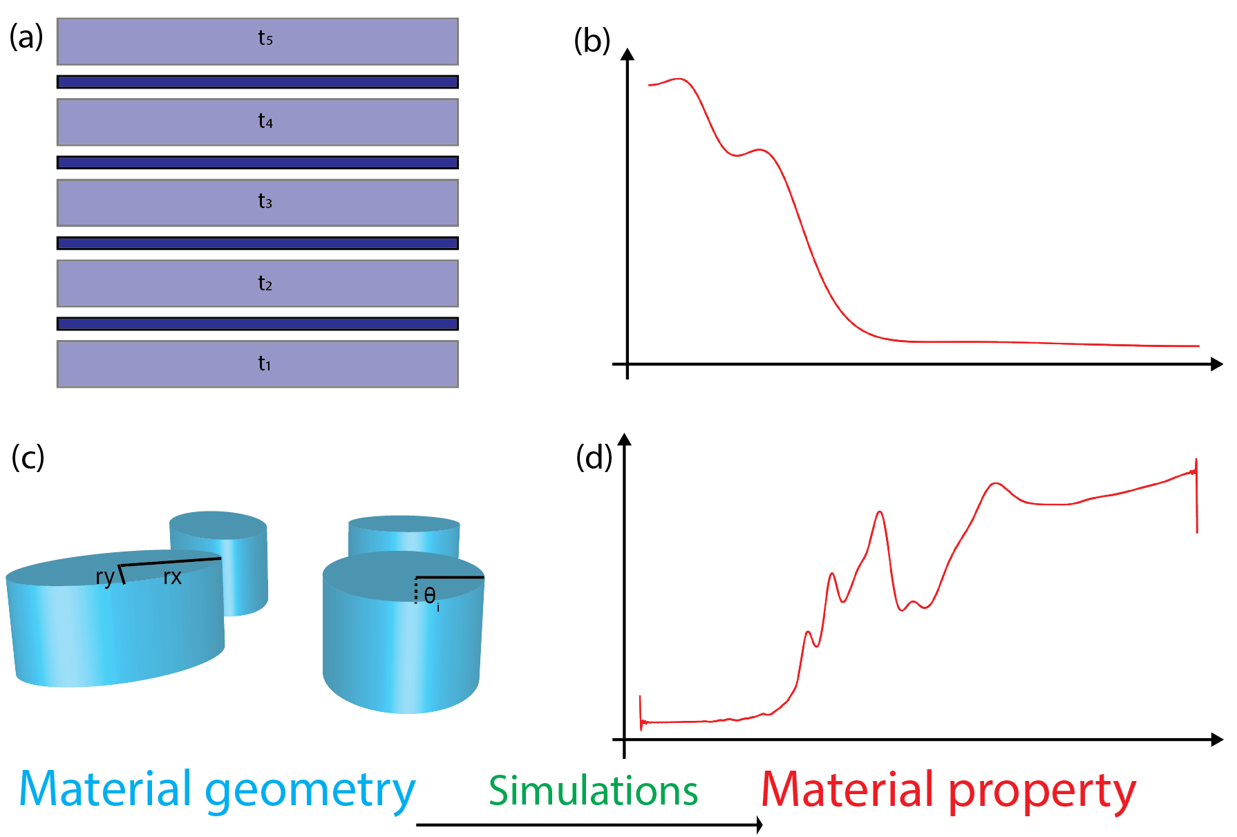
Stacked material (STACK) [38] The goal is to predict the 201-D reflection spectrum of a material based on the thickness of five layers of the material.

Artificial Dielectric Material (ADM) [39] The goal is to predict the 2000-D reflection spectrum of a material based on its 14-D geometric structure. Full wave electromagnetic simulations were utilized in [35] to label data in the original work, requiring 1-2 minutes per input point.

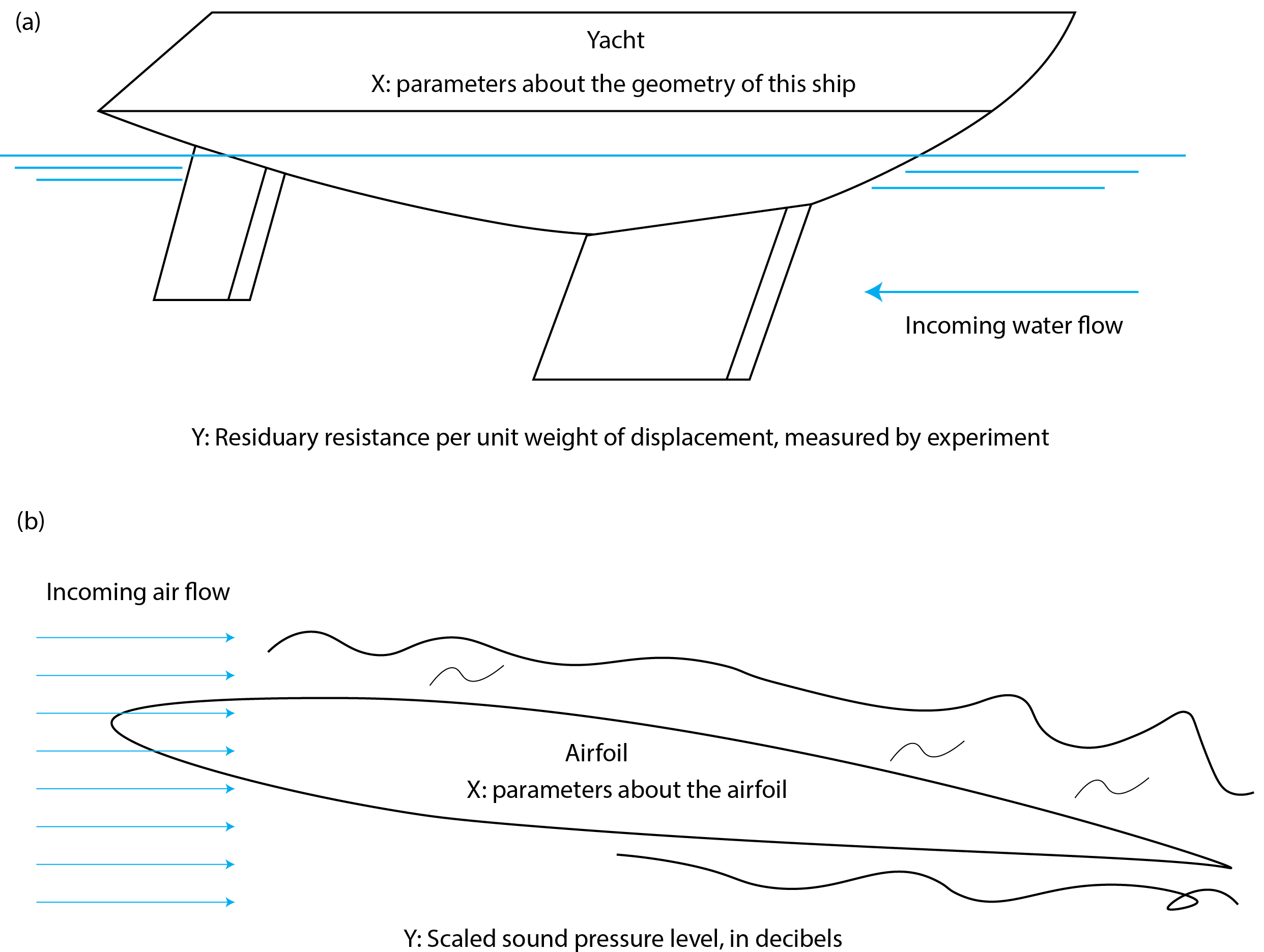
NASA Airfoil (FOIL) [40] The goal is to predict the sound pressure of an airfoil based on the structural properties of the foil, such as its angle of attack and chord length. This problem was published by NASA [41] and the instance labels were obtained from a series of real-world aerodynamic tests in an anechoic wind tunnel. It has been used in other AL literature [42, 43].

Hydrodynamics (HYDR) [40] The goal is to predict the residual resistance of a yacht hull in water based on its shape. This problem was published by the Technical University of Delft, and the instance labels were obtained by real-world experiments using a model yacht hull in the water. It is also referred to as the "Yacht" dataset in some AL literature [23, 26].

Bessel function (BESS) The goal is to predict the value of the solution to Bessel’s differential equation, a second-order ordinary differential equation that is common in many engineering problems. The inputs are the function order $\alpha$ and input position $x$. The order $\alpha$ is limited to non-negative integers below 10.

Damping Oscillator (DAMP) The goal is to predict the full-swing trajectory of a damped oscillator in the first 100 time steps, of the solution to a second-order ordinary differential equation. The input is the magnitude, damping coefficient, and frequency of the oscillation.

Table 2: List of benchmarked methods. $L$ is the labeled set, $Q$ is the already selected query points and $dist$ being L2 distance, $\hat{f}(x)$ is model estimate of $x$, $f(x)$ is oracle label of $x$, $\mu(x)$ is the average of ensemble model output, N is number of models in the model ensemble, $N_{k}$ is the k-nearest-neighbors, $sim$ is cosine similarity, $\phi$ is current model parameter, $\phi^{\prime}$ is the updated parameter, $\mathcal{L}(\phi;(x^{\prime},y^{\prime}))$ is the loss of model with parameter $\phi$ on new labeled data $(x^{\prime},y^{\prime})$, $f_{loss}(x)$ is the auxiliary model that predicts the relative loss,

Method	Abbreviation	Implementation used	Acquisition function (q)
Core-set	GSx	[36]	$\displaystyle\min_{x\in\mathcal{L}\cup\mathcal{Q}}dist(x^{*},x)$
Greedy sampling in y	GSy	[23]	$\displaystyle\min_{y\in\mathcal{L}\cup\mathcal{Q}}dist(\hat{f}(x^{*}),y)$
Improved greedy sampling	GSxy	[23]	$\displaystyle\min_{(x,y)\in\mathcal{L}\cup\mathcal{Q}}dist(x^{*},x)*dist(\hat{f}(x^{*}),y)$
Query by committee	QBC	[14]	$\displaystyle\frac{1}{N}\sum^{N}_{n=1}(\hat{f}_{n}(x)-\mu(x))^{2}$
QBC with diversity	QBCDiv	[14]	$\displaystyle q_{QBC}(x)+q_{div}(x)$
			$\displaystyle(q_{div}(x^{*})=q_{GSx}(x^{*}))$
QBC with diversity	QBCDivDen	[14]	$\displaystyle q_{QBC}(x)+q_{div}(x)+q_{den}(x)$
and density			$\displaystyle(q_{den}(x^{*})=\dfrac{1}{k}\sum_{x\in N_{k}(x^{*})}sim(x^{*},x))$
bayesian by disagreement	BALD	[12]	$\displaystyle q_{QBC}(x)$
Expected model output	EMOC	[30]	$\displaystyle\mathbb{E}_{y^{\prime}|x^{\prime}}\mathbb{E}_{x}||\hat{f}(x;\phi^{\prime})-\hat{f}(x;\phi)||_{1}$
change			$\displaystyle\approx\mathbb{E}_{x}||\nabla_{\phi}\hat{f}(x;\phi)*\nabla_{\phi}\mathcal{L}(\phi;(x^{\prime},y^{\prime}))||_{1}$
Learning Loss	-	[29]	$\displaystyle f_{loss}(x)$
Real loss	MSE	-	$MSE(\hat{f}(x),f(x))$

5 Benchmark Active Learning Methods

From the literature we found ten AL methods that are applicable to (i) regression problems, with (ii) DNN-based regressors, making them suitable for our scientific computing problems. Due to space constraints, we list each method in Table 2 along with key details, and we refer readers to the Supplementary Material for full details. Some of the methods have unique hyper-parameters that must be set by the user. In these cases, we adopt hyperparameter settings suggested by the methods’ authors, shown in Table 2. Upon publication, we will publish software for all of these methods to support future benchmarking.

Note that the last method "MSE" in our benchmark is not an applicable method in real-life scenarios as having the oracle function’s label defeats the purpose of active learning. The purpose of including such a method is to provide an empirical upper bound on the performance of uncertainty sampling DALs that use proxy losses to sample the "low-performance region" of the input space.

6 Benchmark Experiment Design

In our experiments, we will compare ten state-of-the-art DAL methods on eight different scientific computing problems. We evaluate the performance of our DAL methods as a function of $\gamma$ on each of our benchmark problems, with $\gamma\in[2,4,8,16,32,64]$ (i.e., at each step we sample our $U$ with $k*\gamma$ points). Following convention [14, 12], we assume a small training dataset is available at the outset of active learning, $T^{0}$, which has $N_{0}=80$ randomly sampled training instances. We then run each DAL model to $T^{50}$ AL steps, each step identifying $k=40$ points to be labeled from a fresh, randomly generated pool of size $k*\gamma$. For each benchmark problem, we assume an appropriate neural network architecture is known apriori. Each experiment (i.e., the combination of dataset, DAL model, and $\gamma$ value) is run 5 times to account for randomness. The performance MSE is calculated over a set of 4000 test points that are uniformly sampled within the $x$-space boundary.

We must train a regression model for each combination of problem and DAL method. Because some DAL methods require an ensemble model (e.g., QBC), we use an ensemble of 10 DNNs as the regressor for all of our DAL algorithms(except for the ADM problem, which is set to 5 due to the GPU RAM limit). More details of the models used and training procedures can be found in the supplementary materials.

Due to the space constraints, we summarize our DAL performance by the widely-used area under curve (AUC) of the error plot [12, 43, 23]. We report the full MSE vs # labeled point plots in the supplementary material. For the AUC calculation, we used ’sklearn.metrics.auc’ [44] then further normalized by such AUC of random sampling method. All below results are given in the unit of normalized AUC of MSE ($nAUC_{MSE})$.

7 Experimental Results

Figure 3: The performance of each DAL method (x-axis) in terms of $nAUC_{MSE}$ (y-axis). For each of the DAL method, we report a bar indicating the range of $nAUC_{MSE}$ values obtained as we vary the pool ratio, $\gamma\in[2,4,...,64]$; for a given DAL method, we report one bar for each of the eight benchmark problems, indicated by a unique color in the legend. Each bar is bisected by a solid black and magenta line, respectively. The black line represents the average $nAUC_{MSE}$ value across all settings of $\gamma$. The magenta line represents the performance using $\gamma_{prior}$ (see Sec. 7 for details). The dashed red line at $nAUC_{MSE}=1$ corresponds to the performance obtained using random sampling. Note that some vertical bars are clipped at the top; this was done intentionally to improve the visualization overall.

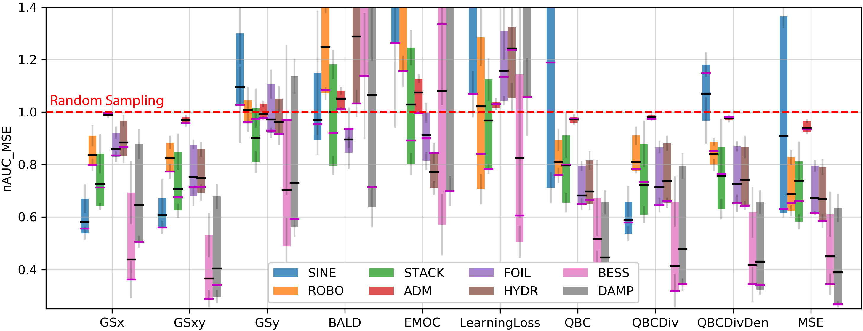
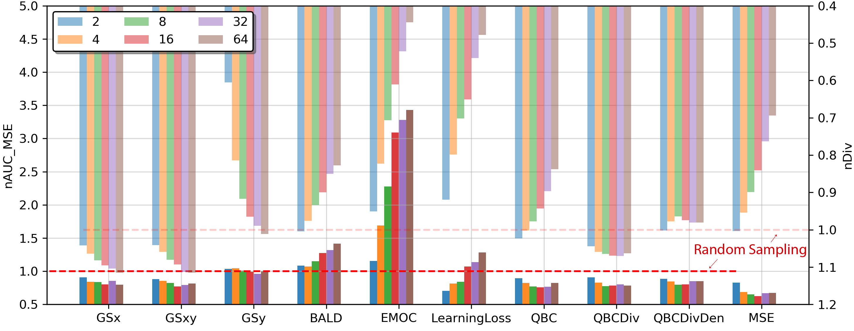
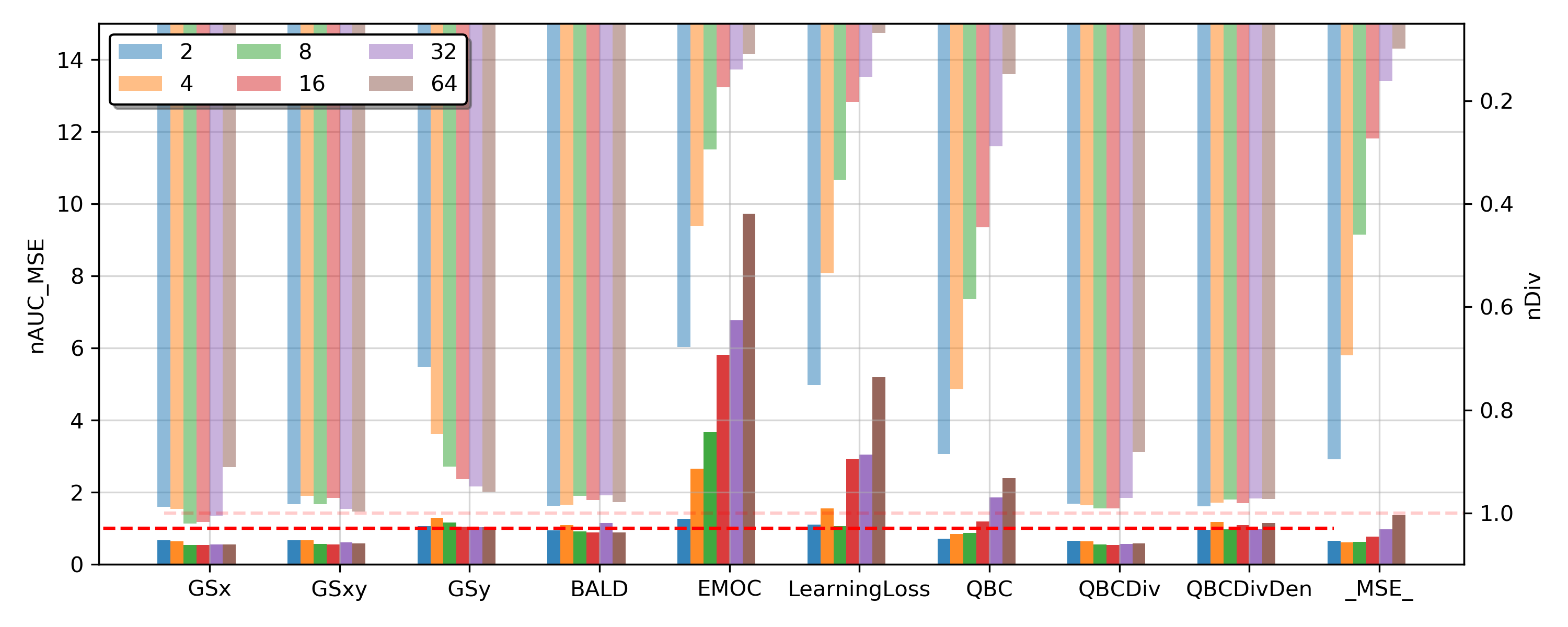
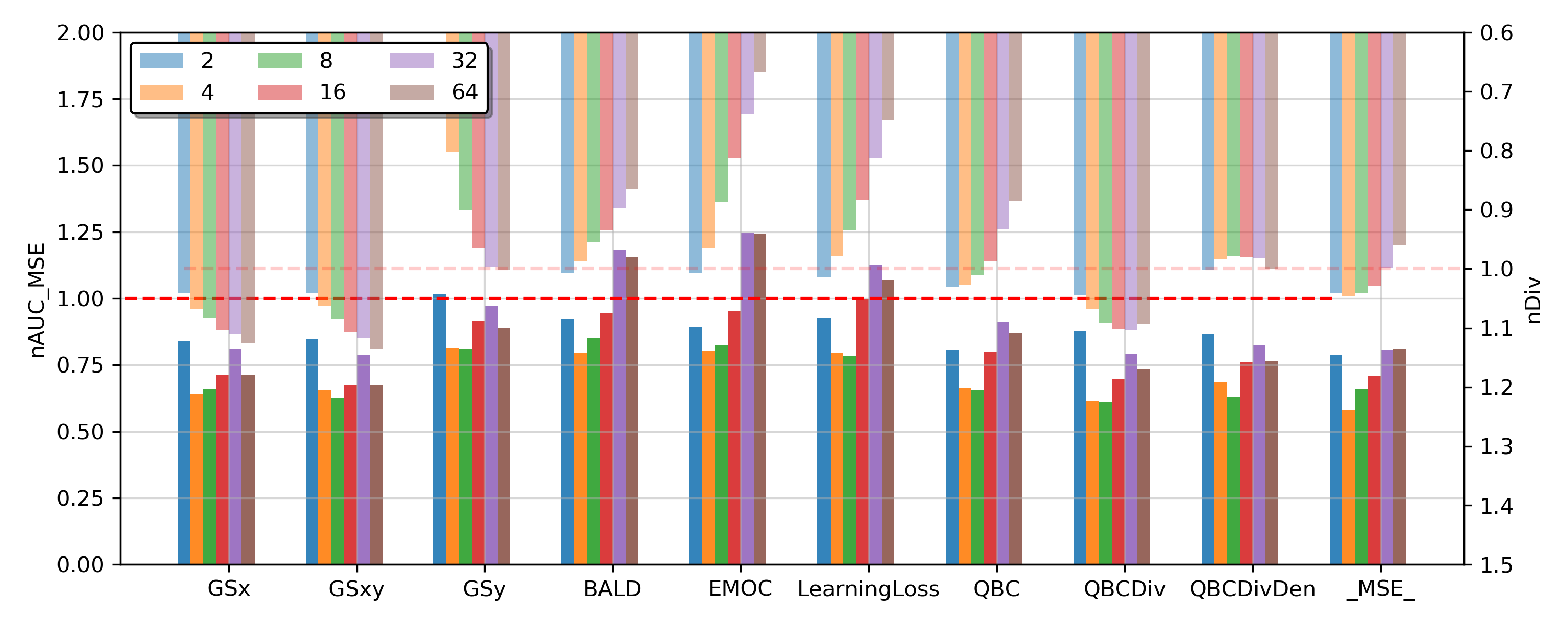
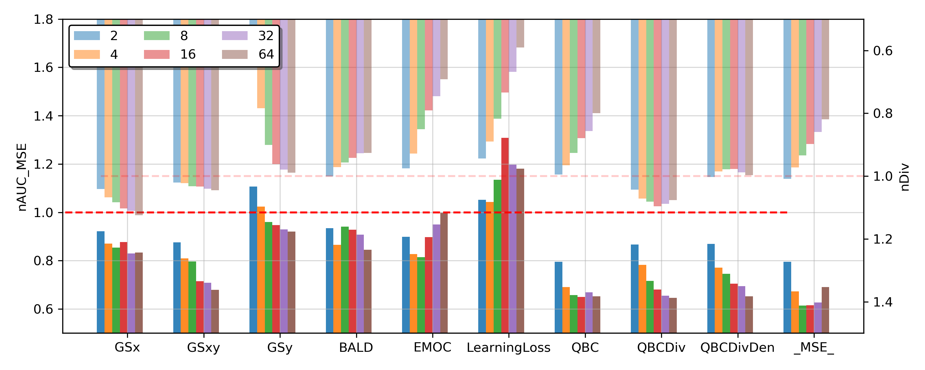
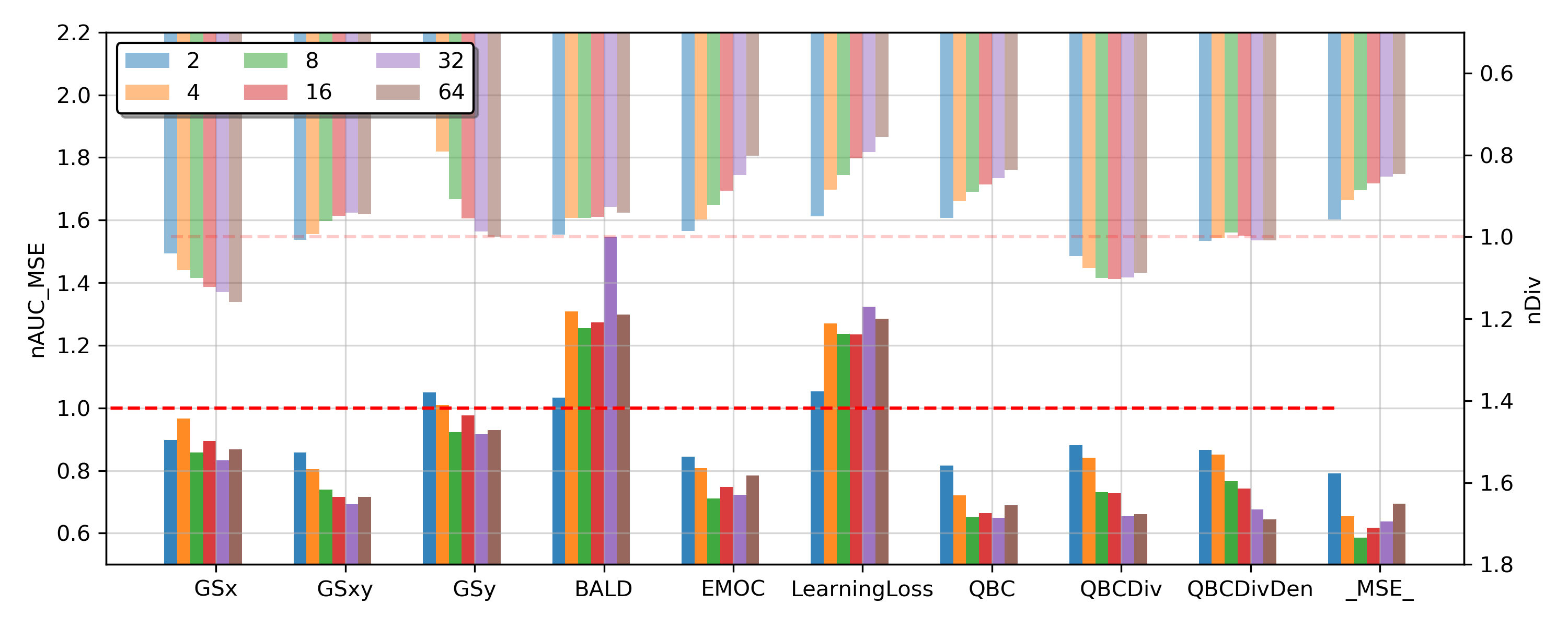
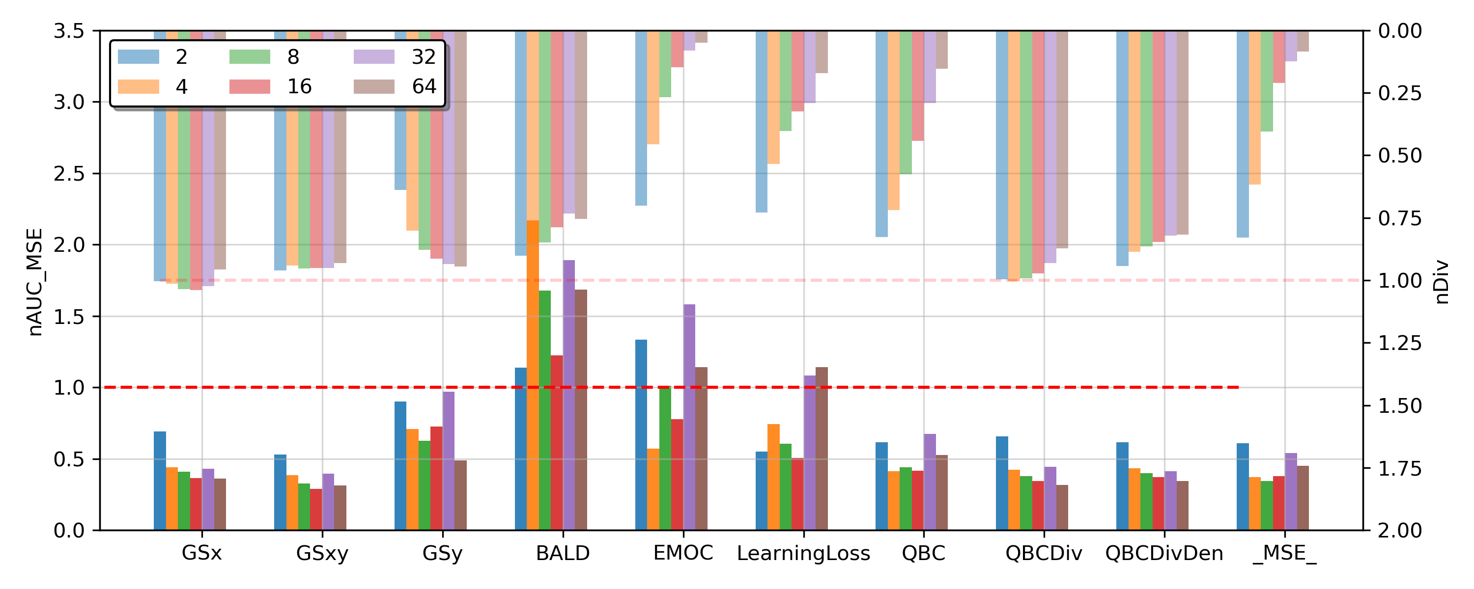
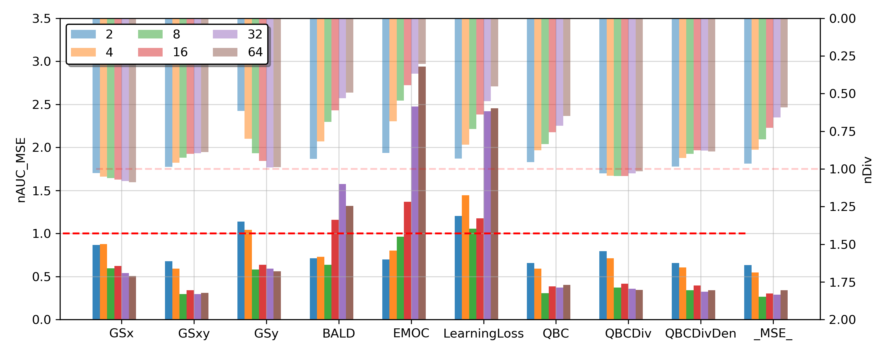
The performance of all ten DAL methods on all eight benchmark datasets is summarized in Fig 3. The y-axis is the normalized $nAUC_{MSE}$ and the x-axis is the DAL methods of interest and the color code represents the different benchmark datasets. The horizontal red dashed line represents the performance of random sampling, which by definition is equal to one (see Sec. 6). Further details about Fig. 3 are provided in its caption. We next discuss the results, with a focus on findings that are most relevant to DAL in the wild.

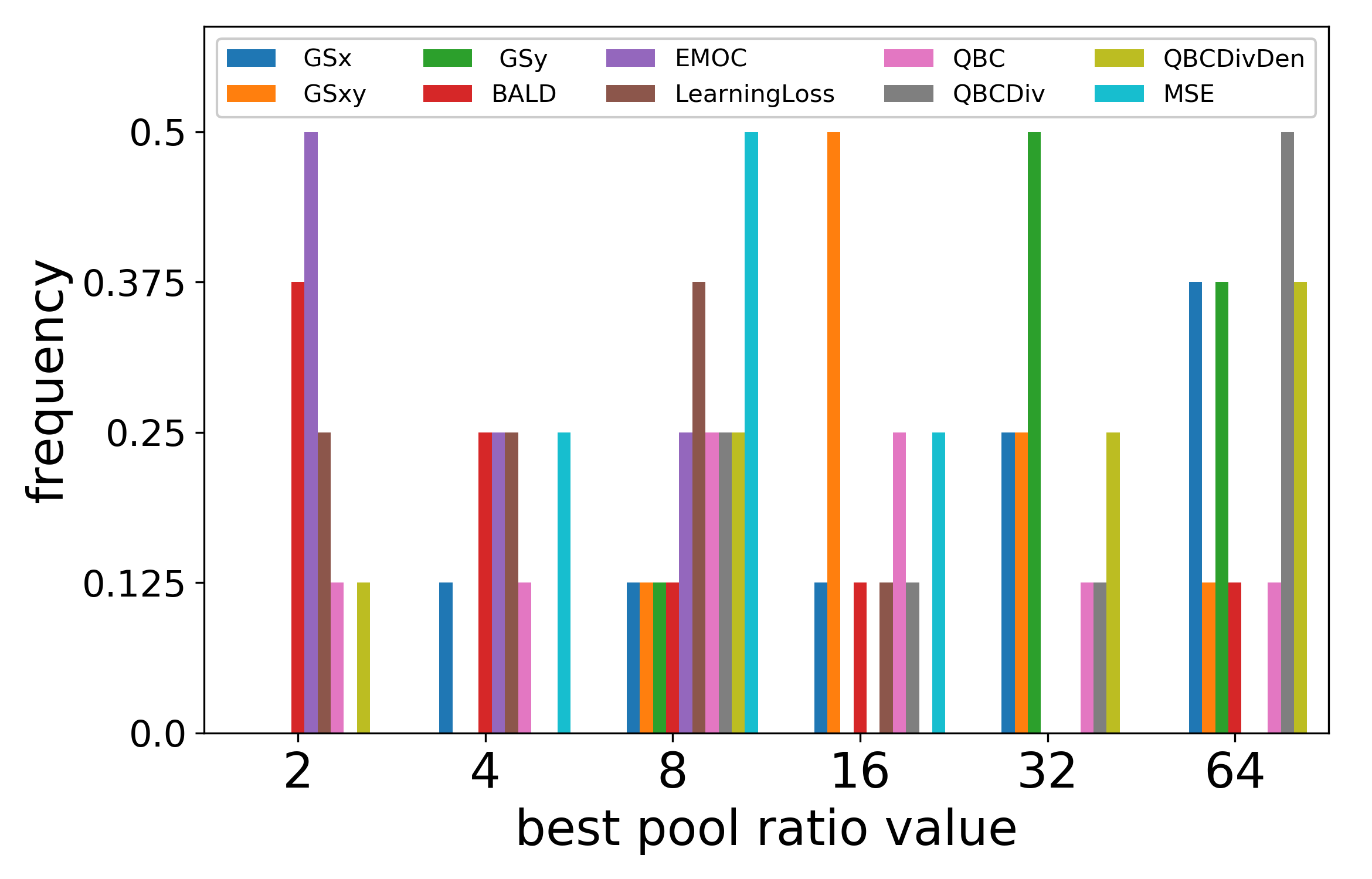
(i) DALs are sensitive to their pool ratio, $\gamma$ The results in Fig. 3 indicate that all of our benchmark DAL methods are sensitive to their setting of $\gamma$ - a central hypothesis of this work. As indicated by the vertical bars in Fig. 3, the $nAUC_{MSE}$ obtained by each DAL method varies substantially with respect to $\gamma$. For most of the DAL methods, there exist settings of $\gamma$ (often many) that cause them to perform worse than random sampling. This has significant implications for DAL in the wild since, to our knowledge, there is no general method for estimating a good $\gamma$ setting prior to collecting large quantities of labeled data (e.g., to run trials of DAL with different $\gamma$ settings), defeating the purpose of DAL. Furthermore, there is no single setting of $\gamma$ that works well across all of our benchmark problems. In Fig. 4 we present a histogram of the best $\gamma$ setting for each DAL method. The results indicate that the best $\gamma$ parameter depends strongly upon both the DAL method being used, and the particular benchmark problem. More importantly, there is no DAL method such that a single setting of $\gamma$ performs best across all benchmark problems. Therefore, in the wild, there is uncertainty regarding the best setting of $\gamma$ and therefore the (i) performance one can expect from DAL methods, and (ii) even whether it will perform better than random sampling.

(ii) Do DAL methods outperform random sampling in the wild? The results indicate that several DAL methods tend to obtain much lower $nAUC_{MSE}$, on average, than random sampling. This includes methods such as GSx, GSxy, GSy, QBC, QBCDiv, and QBCDivDen. The results therefore suggest that these methods are beneficial more often than not, compared to random sampling - an important property. However, as discussed in Sec. 7(i), all DAL methods exhibit significant performance variance with respect to $\gamma$, as well as the particular problem of interest. Consequently, many of the aforementioned subset of methods can still often perform worse than random sampling. For example, this is the case of QBC, GSy, and QBCDivDen on the SINE problem. In many real-world settings, especially in scientific computing scenarios, the cost of collecting labels can be high and the risks associated with poor DAL performance may deter its use. Therefore, another important criteria is performance robustness: do any DAL methods consistently perform better than random sampling, in the wild, when $\gamma$ is unknown? Our results indicate that GSx, GSxy, and QBCDiv always outperform at least as well as random sampling, and often substantially better, regardless of the problem setting or the setting of $\gamma$.

Note that all three robust DALs (GSx, GSxy, QBCDiv) has x-space diversity in their loss function. As we show more evidence in Sec. 7.2 that worse than random performance highly correlates with mode collapse (i.e. lack of x-space diversity), we conclude that diversity in x-space is a crucial factor contributing towards DAL robustness in the current setting. The only DAL that considers diversity but did not show robustness is QBCDivDen. We attribute this failure in robustness to the lower weight on diversity due to the addition of the new density metric.

(iii) Are some problems inherently not suitable for DAL? Our results indicate that some problems seem to benefit less from DAL than others. For example, the average performance of our ten DAL methods varies substantially across problems - this is visually apparent in Fig. 3. It is possible that some problems have unique statistical properties that make them ill-suited for most DAL methods. Even if we only consider the best-performing DAL method for each benchmark problem, we still see substantial differences in achievable performance across our problems. A notable example is the ADM problem, where the best-performing DAL method achieves $nAUC_{MSE}$ $>$ 0.9, which is only slightly better than random sampling. By contrast, the best performing DAL method for the BESS and DAMP problems achieve $nAUC_{MSE}\approx 0.3$. These results suggest that some problems may have properties that make DAL (and perhaps AL in general) inherently difficult, or unhelpful. Understanding these properties may reveal useful insights about AL methods, and when they should be applied; we propose this a potential area of future work.

Figure 4: The histogram (frequency) of the best pool ratio values found in each of the DALs. For a particular DAL method, this figure shows the frequency (% out of 8) that a particular pool ratio (x-axis) performs the best in terms of average $nAUC_{MSE}$ metric.

Figure 5: A representative, combined plot with $nAUC_{MSE}$ performance (bottom, y-axis at left, solid) and collapse metric,nDiv (upper, y-axis at right, more transparent) for each of the ten DAL models at all pool ratio (color coded) for robotic arm dataset (ROBO). Dashed horizontal red lines starting from both $y$ axes represent the random sampling’s average $nAUC_{MSE}$ and nDiv at 1.

7.1 Knowledge about optimal pool ratio

The robustness of DALs with respect to different pool ratios would not be a problem if the practitioners can find a good performing pool ratio for a single DAL method (dataset is always considered unknown in AL as no labeled data is available). Fig 4 shows the histogram of the optimal pool ratio values among the eight datasets. Immediately we can see that the maximum frequency of the best pool ratio of all ten DALs is 0.5 (4 out of 8 datasets perform best under this pool ratio), which means there is no dominating pool ratio for any of the benchmarked DAL methods. Furthermore, if we take the best pool ratio from Fig 4 (winning in most datasets, break a tie randomly) and apply this pool ratio across all datasets, we get the performance of the ’best overall’ pool ratio (magenta line in bars) shown in Fig 3. Nearly all magenta lines are better than the black lines, showing the value of having good previous benchmark knowledge about a wise choice of pool ratio. However, the robustness issue is still present as only the MSE method became robust with the extra knowledge.

7.2 Mode collapse analysis

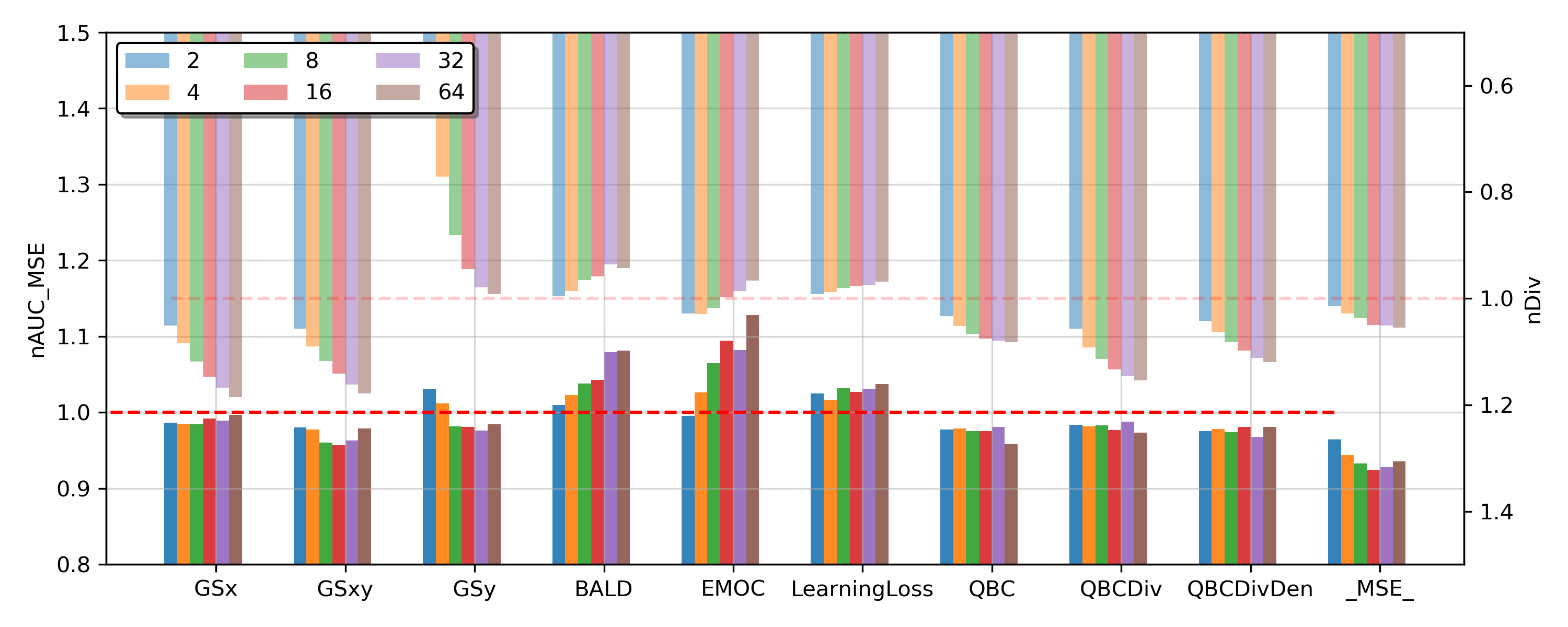
As one hypothesis of failure of DALs is the mode collapse issue due to lack of diversity. We calculated the diversity metric as the average nearest neighbor distance

$$Div=\dfrac{1}{|T|}\sum_{t}^{T}\dfrac{1}{K}\sum_{i}^{K}\min_{x^{*}\in\mathcal{Q^{T}}}dist(x^{*},x^{i})$$

where $\mathcal{Q}^{t}$ represents the queried batch at active learning step $t$ and $|T|=50$ is the total number of active learning steps. Note that this metric is similar to, but not a simple average of $q_{GSx}(x)$ as $Div$ only focuses on per batch diversity and does not take the labeled set into consideration. It is also further normalized ($nDiv$) by the value of random sampling for each dataset separately. The lower this metric’s value, the more severe the mode collapse issue would be.

The $nDiv$ is plotted at the top half of Fig 5 using the inverted right y-axis. For the obvious failure cases (BALD, EMOC and Learning Loss) in this particular dataset (their $nAUC_{MSE}$ exceeds 1), a clear trend of mode collapse can be observed at the upper half of the plot (nDiv much lower than 1). Meanwhile, a strong correlation between the pool ratio and the diversity metric can be observed: (i) For all GS methods, as they seek to maximize diversity their diversity increases monotonically with larger pool ratio. (ii) For uncertainty-based methods (BALD, EMOC, LearningLoss, QBC, MSE), as they seek to maximize uncertainty, their diversity decreases monotonically with larger pool ratios. (iii) For combined methods like QBCDiv and QBCDivDen, the relationship between pool ratio and diversity does not observe a strong correlation.

8 Conclusion

In conclusion, for the first time in the literature, we benchmarked ten state-of-the-art deep active learning methods on eight benchmark datasets for scientific computing regression scenarios. It shed light on an important, surprising discovery that a lot of pool-based DALs are not robust compared to random sampling under scientific computing scenarios when no pre-defined pool is given. Furthermore, we showed that the value of a good-performing pool ratio is problem dependent and hence hard to obtain in advance. We also analyzed the failure mode of the DALs, and discovered a strong correlation between lack of diversity ($x$-space mode-collapse) and lack of robustness and suggested that in future scientific computing scenarios practitioners should always employ $x$-space diversity in their DAL method to curb such mode collapse.

Appendix A Details of the benchmarking methods

Core-set (GSx: Greedy sampling in $x$ space) [36]. This approach only relies upon the diversity of points in the input space, $\mathcal{X}$, when selecting new query locations. A greedy selection criterion is used, given by

$$q_{GSx}(x^{*})=\min_{x\in\mathcal{L}\cup\mathcal{Q}}dist(x^{*},x)$$

where $\mathcal{L}$ is the labeled set, $\mathcal{Q}$ is the already selected query points and $dist$ being L2 distance.

Greedy sampling in $y$ space (GSy) [23]. Similar to GSx which maximizes diversity in the $x$ space in a greedy fashion, GSy maximizes the diversity in the $y$ space in a greedy fashion:

$$q_{GSy}(x^{*})=\min_{y\in\mathcal{L}\cup\mathcal{Q}}dist(f(x^{*}),y)$$

where $f(x)$ is the current model prediction of the $x$ and $y$ is the labels in the already labeled training set plus the predicted labels for the points (to be labeled) selected in the current step.

Greedy sampling in xy space (GSxy) [23]. Named as ’Improved greedy sampling (iGS)’ in the original paper [23], this approach combines GSx and GSy and uses multiplication of the distance of both $x$ and $y$ space in its acquisition function:

$$q_{GSxy}(x^{*})=\min_{(x,y)\in\mathcal{L}\cup\mathcal{Q}}dist(x^{*},x)*dist(f(x^{*}),y)$$

Query-by-committee (QBC) [45] The QBC approach is pure uncertainty sampling given by Alg. 1 if we set $q(x)=q_{QBC}(x)$:

$$q_{QBC}(x)=\frac{1}{N}\sum^{N}_{n=1}(\hat{f}_{n}(x)-\mu(x))^{2}$$

Here $\hat{f}_{n}$ denotes the $n^{th}$ model in an ensemble of $N_{ens}$ models (DNNs in our case), and $\mu(x)$ is the mean of the ensemble predictions at $x$. In each iteration of AL these models are trained on all available training data at that iteration.

QBC with diversity (Div-QBC) [14]. This method improves upon QBC by adding a term to $q$ that also encourages the selected query points to be diverse from one another. This method introduces a hyperparameter for the relative weight of the diversity and QBC criteria and we use an equal weighting ($\alpha=0.5$ [14]).

$$q_{QBCDiv}(x) =(1-\alpha)*q_{QBC}(x)+\alpha*q_{div}(x)$$

$$q_{div}(x^{*}) =q_{GSx}(x^{*})$$

QBC with diversity and density (DenDiv-QBC) [14]. This method builds upon Div-QBC by adding a term to $q(x)$ that encourages query points to have uniform density. This method introduces two new hyperparameters for the relative weight ($\alpha=\beta=\dfrac{1}{3}$) of the density, diversity, and QBC criteria, and we use an equal weighting as done in the original paper [14].

$$q_{QBCDivDen}(x) =(1-\alpha-\beta)*q_{QBC}(x)$$

$$+\alpha*q_{div}(x)+\beta*q_{den}(x)$$

$$q_{den}(x^{*}) =\dfrac{1}{k}\sum_{x\in N_{k}(x^{*})}sim(x^{*},x)$$

where $N_{k}(x^{*})$ is the k nearest neighbors of an unlabeled point, $sim(x^{*},x)$ is the cosine similarity between points.

Bayesian active learning by disagreement (BALD) [12]. BALD uses the Monte Carlo dropout technique to produce multiple probabilistic model output to estimate the uncertainty of model output and uses that as the criteria of selection (same as $q_{QBC}(x)$). We used 25 forward passes to estimate the disagreement.

Expected model output change (EMOC) [13, 30]. EMOC is a well-studied AL method for the classification task that strives to maximize the change in the model (output) by labeling points that have the largest gradient. However, as the true label is unknown, some label distribution assumptions must be made. Simple approximations like uniform probability across all labels exist can made for classification but not for regression tasks. [30] made an assumption that the label is simply the average of all predicted output in the unlabeled set ($y^{\prime}(x^{\prime})=\mathbb{E}_{x\in\mathcal{U}}f(x)$) and we use this implementation for our benchmark of EMOC.

$$q_{EMOC}(x^{\prime}) =\mathbb{E}_{y^{\prime}|x^{\prime}}\mathbb{E}_{x}||f(x;\phi^{\prime})-f(x;\phi)||_{1}$$

$$\approx\mathbb{E}_{x}||\nabla_{\phi}f(x;\phi)*\nabla_{\phi}\mathcal{L}(\phi;(x^{\prime},y^{\prime}))||_{1}$$

where $f(x;\phi)$ is the current model output for point $x$ with model parameter $\phi$, $\phi^{\prime}$ is the updated parameter after training on labeled point x’ with label y’ and $\mathcal{L}(\phi;(x^{\prime},y^{\prime})$ is the loss of the model with current model parameter $\phi$ on new labeled data $(x^{\prime},y^{\prime})$.

Learning Loss [29]. Learning Loss is another uncertainty-based AL method that instead of using proxies calculated (like variance), learns the uncertainty directly by adding an auxiliary model to predict the loss of the current point that the regression model would make. The training of the auxiliary model concurs with the main regressor training and it uses a soft, pair-wise ranking loss instead of Mean Squared Error (MSE) loss to account for the fluctuations of the actual loss during the training.

$$q_{LL}(x)=f_{loss}(x)$$

where $f_{loss}(x)$ is the output of the loss prediction auxiliary model. In this AL method, there are multiple hyper-parameters (co-training epoch, total auxiliary model size, auxiliary model connections, etc.) added to the AL process, all of which we used the same values in the paper if specified [29].

Infeasible uncertainty upper bound: Real loss (MSE). As uncertainty-based AL methods generally follow the philosophy of "uncertain $\approx$ high loss $\approx$ more valuable if labeled" and constructed various proxy to approximate MSE , one kind of upper bound of such AL philosophy is to use the real (MSE) loss as its acquisition criteria:

$$q_{MSE}(x)=MSE(f(x),oracle(x))$$

Note that this method would never be possible in actual applications as it needs real labels of unlabeled points to calculate its acquisition function, hence defeating the purpose of AL. Nevertheless, this serves as a good, general upper bound of the uncertainty-based model (a strict upper bound for Learning Loss AL) and helps us understand the modality of DAL performance.

Appendix B Details of benchmark datasets used

1D sine wave (Wave). A noiseless 1-dimensional sinusoid with varying frequency over $x$, illustrated in Img 6.

$$y=x*sin(a_{1}*sin(a_{2}*x)),$$

where $a_{1}=3$ and $a_{2}=30$ is chosen to make a relative complicated loss surface for the neural network to learn while also having a difference in sensitivity in the domain of x.

2D robotic arm (Arm), [37] In this problem we aim to predict the 2D spatial location of the endpoint of a robotic arm based on its joint angles. Illustrated in Img 6. The Oracle function is given by

$$y_{0}=\sum_{i=1}^{3}\cos(\dfrac{pi}{2}x_{i})*l_{i},y_{1}=x_{0}+\sum_{i=1}^{3}\sin(\dfrac{pi}{2}x_{i})*l_{i}$$

where $y$ is the position in the 2D plane, $x_{0}$ is the adjustable starting horizontal position, $x_{i=1,2,3}$ are the angles of the arm relative to horizontal reference and $l_{i=0,1,2}=[0.5,0.5,1]$ represents the i-th length of the robotic arm component.

Figure 6: Schematic illustration of sine wave and robotic arm datasets

Stacked material (Stack),[38]. In this problem, we aim to predict the reflection spectrum of a material, sampled at 201 wavelength points, based upon the thickness of each of the 5 layers of the material, illustrated in Fig 7. It was also benchmarked in [46]. An analytic Oracle function is available based upon physics[38].

Artificial Dielectric Material (ADM), [39] This problem takes the geometric structure of a material as input, and the reflection spectrum of the material, as a function of frequency, illustrated in Fig 7. It was also benchmarked in [35]. This dataset consists of input space of 3D geometric shape parameterized into 14 dimension space and the output is the spectral response of the material. The oracle function is a DNN [35].

Figure 7: (a, c) are schematic illustration of two material design datasets (Stack & ADM). (b, d) are example spectra of their material property after simulations from their geometric parameterization (typically from Maxwell equation solvers that are slow and hence can benefit from active learning)

NASA Airfoil (Foil), [40] NASA dataset published on https://archive.ics.uci.edu/ml/datasets/airfoil+self-noise UCI ML repository[40] obtained from a series of aerodynamic and acoustic tests of 2D/3D airfoil blade sections conducted in an anechoic wind tunnel, illustrated in Fig 8. The input is the physical properties of the airfoil, like the angle of attack and chord length and the regression target is the sound pressure in decibels. We use a well-fitted random forest fit to the original dataset as our oracle function following prior work[47]. The fitted random forest architecture and its weights are also shared in our code repo to ensure future work makes full use of such benchmark datasets as we did.

Hydrodynamics (Hydro). [40] Experiment conducted by the Technical University of Delft, illustrated in Fig 8, (hosted by https://archive.ics.uci.edu/ml/datasets/Yacht+HydrodynamicsUCI ML repository[40]), this dataset contains basic hull dimensions and boat velocity and their corresponding residuary resistance. Input is 6 dimensions and output is the 1 dimension. We use a well-fitted random forest fit to the original dataset as our oracle function. The fitted random forest architecture and its weights are also shared in our code repo to ensure future work makes full use of such benchmark dataset as we did.

Figure 8: Schematic illustration of Airfoil and Hydro experiments. Reproduced from the original source of experiment reports from NASA and Delft University of technology. (a) The Hydro experiment with an actual yacht being built and resistance was measured in a water flow experiment as the regression target y. (b) Airfoil experiment where input is the parameters of the airfoil and the sound pressure level is measured as target $y$ of the regression task.

Bessel equation The solution to the below single dimension second-order differential equation:

$$x^{2}\dfrac{d^{2}y}{dx^{2}}+x\dfrac{dy}{dx}+(x^{2}-\alpha^{2})y=0$$

where input is $\alpha$ and $x$ position given. $\alpha$ is limited to non-negative integers smaller than 10 and $x\in[0,10]$. The solution examples can be visualized in Fig 9. Our choice of $\alpha$ values makes the Bessel functions cylinder harmonics and they frequently appear in solutions to Laplace’s equation (in cylindrical systems). The implementation we used is the python package ’scipy.special.jv(v,z)’ [48].

Damping oscillator equation The solution to the below ordinary second-order differential equation:

$$m\dfrac{dx^{2}}{d^{2}t}+b\dfrac{dx}{dt}+\dfrac{mg}{l}x=0$$

where m is the mass of the oscillator, b is the air drag, g is the gravity coefficient, l is the length of the oscillator’s string and it has analytical solution of form

$$x=ae^{-bt}cos(\alpha-\psi)$$

where a is the amplitude, b is the damping coefficient, $\alpha$ is the frequency and $\psi$ is the phase shift. We assume $\psi$ to be 0 and let a,b,$\alpha$ be the input parameters. The output, unlike our previous ODE dataset, is taken as the first 100 time step trajectory of the oscillator, making it a high dimensional manifold (nominal dimension of 100 with true dimension of 3). The trajectory is illustrated in Fig 9. We implement the above solution by basic python math operations.

Figure 9: Schematic illustration of Bessel function solution and the damping oscillator solutions.

Appendix C List of pool ratio used in existing literature

17000 [49], 20 to 2000 [14], 300 to 375[50], 11-20 [11], 1000 [33], and 1 to 11 [51].

Appendix D Details of models training and architecture

In the below table  3, we present the model architecture for each of our benchmarked datasets. Unless otherwise noted, all of them are fully connected neural networks.

Table 3: Regression model, $\hat{f}$ architecture details for each problem. *: for ADM, there are 3 layers of convolutions after the linear layer)

Feat	Sine	Robo	Stack	ADM	Foil	Hydr	BESS	DAMP
NODE	20	500	700	1500	200	50	50	500
LAYER	9	4	9	$4^{*}$	4	6	6	6

We implemented our models in Pytorch [52]. Beyond the above architectural differences, the rest of the model training settings are the same across the models: Starting labeled set of size 80, in each step DAL finds 40 points to be labeled for 50 active learning steps. Each regression model is an ensemble network of 10 models of size illustrated in Tbl 1 except the ADM dataset (5 instead of 10 due to RAM issue). The test dataset is kept at 4000 points uniformly sampled across the $x$-space and they are fixed the same across all experiments for the same dataset. No bootstrapping is used to train the ensemble network and the only source of difference between networks in the ensemble (committee) is the random initialization of weights.

The batch size is set to be 5000 (larger than the largest training set) so that the incomplete last batch would not affect the training result (as we sample more and more data, we can’t throw away the last incomplete batch but having largely incomplete batch de-stabilizes training and introduce noise into the experiment. Adam optimizer is used with 500 training epochs and the model always retrains from scratch. (We observe that the training loss is much higher if we inherit from the last training episode and do not start from scratch, which is consistent with other literature [21]). The learning rate is generally 1e-3 (some datasets might differ), and the decay rate of 0.8 with the decay at the plateau training schedule. The regularization weight is usually 1e-4 (dataset-dependent as well). The hyper-parameters only change with respect to the dataset but never with respect to DAL used.

The hyperparameters are tuned in the same way as the model architecture: Assume we have a relatively large dataset (2000 randomly sampling points) and tune our hyperparameter on this set. This raises another robustness problem of deep active learning, which is how to determine the model architecture before we have enough labels. This is currently out of the scope of this work as we focused on how different DALs behave with the assumption that the model architectures are chosen smartly and would be happy to investigate this issue in future work.

For the BALD method, we used a dropout rate of 0.5 as advised by previous work. As BALD requires a different architecture than other base methods (a dropout structure, that is capable of getting a good estimate even with 50% of the neurons being dropped), the model architecture for the active learning is different in that it enlarges each layer by a constant factor that can make it the relatively same amount of total neurons like other DAL methods. Initially, the final trained version of the dropout model is used as the regression model to be evaluated. However, we found that an oversized dropout model hardly fits as well as our ensembled counterpart like other DAL methods. Therefore, to ensure the fairness of comparison, we trained another separate, ensembled regression model same as the other DALs and reported our performance on that.

For the LearningLoss method, we used the same hyper-parameter that we found in the cited work in the main text: relative weight of learning loss of 0.001 and a training schedule of 60% of joint model training and the rest epoch we cut the gradient flow to the main model from the auxiliary model. For the design of the auxiliary model, we employed a concatenation of the output of the last three hidden layers of our network, each followed by a fully connected network of 10 neurons, before being directed to the final fully connected layer of the auxiliary network that produces a single loss estimate.

For the EMOC method, due to RAM limit and time constraint, we can not consider all the model parameters during the gradient calculation step (For time constraint, table 4 gives a good reference of how much longer EMOC cost, even in this reduced form). Therefore, we implemented two approximations: (i) For the training set points where the current model gradients are evaluated, instead of taking the ever-growing set that is more and more biased towards the DAL selection, we fixed it to be the 80 original, uniformly sampled points. (ii) We limit the number of model parameters to evaluate the EMOC criteria to 50k. We believe taking the effect of 50 thousand parameters gives a good representation of the model’s response (output change) for new points. We acknowledge that these approximations might be posing constraints to EMOC, however, these are practical, solid challenges for DAL practitioners as well and these are likely the compromise to be made during application.

D.1 Computational resources

Here we report the computational resources we used for this work: AMD CPU with 64 cores; NVIDIA 3090 GPU x4 (for each of the experiment we used a single GPU to train); 256GB RAM.

Appendix E Additional performance plots

As the benchmark conducts a huge set of experiments that are hard to fit in the main text, here we present all the resulting figures for those who are interested to dig more takeaways.

E.1 Time performance of the benchmarked DAL methods

We also list the time performance of each DAL method, using the ROBO dataset as an example in the below table 4. Note that this is only the sampling time cost, not including the model training time, which is usually significantly larger than the active learning sampling time at each step. The only DAL method that potentially has a time performance issue is the EMOC method, which requires the calculation of each of the gradients with respect to all parameters and therefore takes a much longer time than other DAL methods. However, as it is shown in the main text that it is not a robust method in our setting, there is no dilemma of performance/time tradeoff presented here.

Table 4: Time performance for average time spent during the sampling and labeling process for ROBO dataset per active learning step (40 points) in microseconds. LL: LearningLoss

Dataset	Random	GSx	GSxy	GSy	BALD	EMOC	LL	QBC	QBCDiv	QBCDivDen	MSE
Time	1.98	4.61	6.74	5.28	8.00	707	5.96	4.02	6.76	7.93	1.99

E.2 Combined plot with $nAUC_{MSE}$ and nDiv

Figure 10: $nAUC_{MSE}$ and nDiv plot for SINE

Figure 11: $nAUC_{MSE}$ and nDiv plot for STACK

Figure 12: $nAUC_{MSE}$ and nDiv plot for ADM

Figure 13: $nAUC_{MSE}$ and nDiv plot for FOIL

Figure 14: $nAUC_{MSE}$ and nDiv plot for HYDR

Figure 15: $nAUC_{MSE}$ and nDiv plot for BESS

Figure 16: $nAUC_{MSE}$ and nDiv plot for DAMP

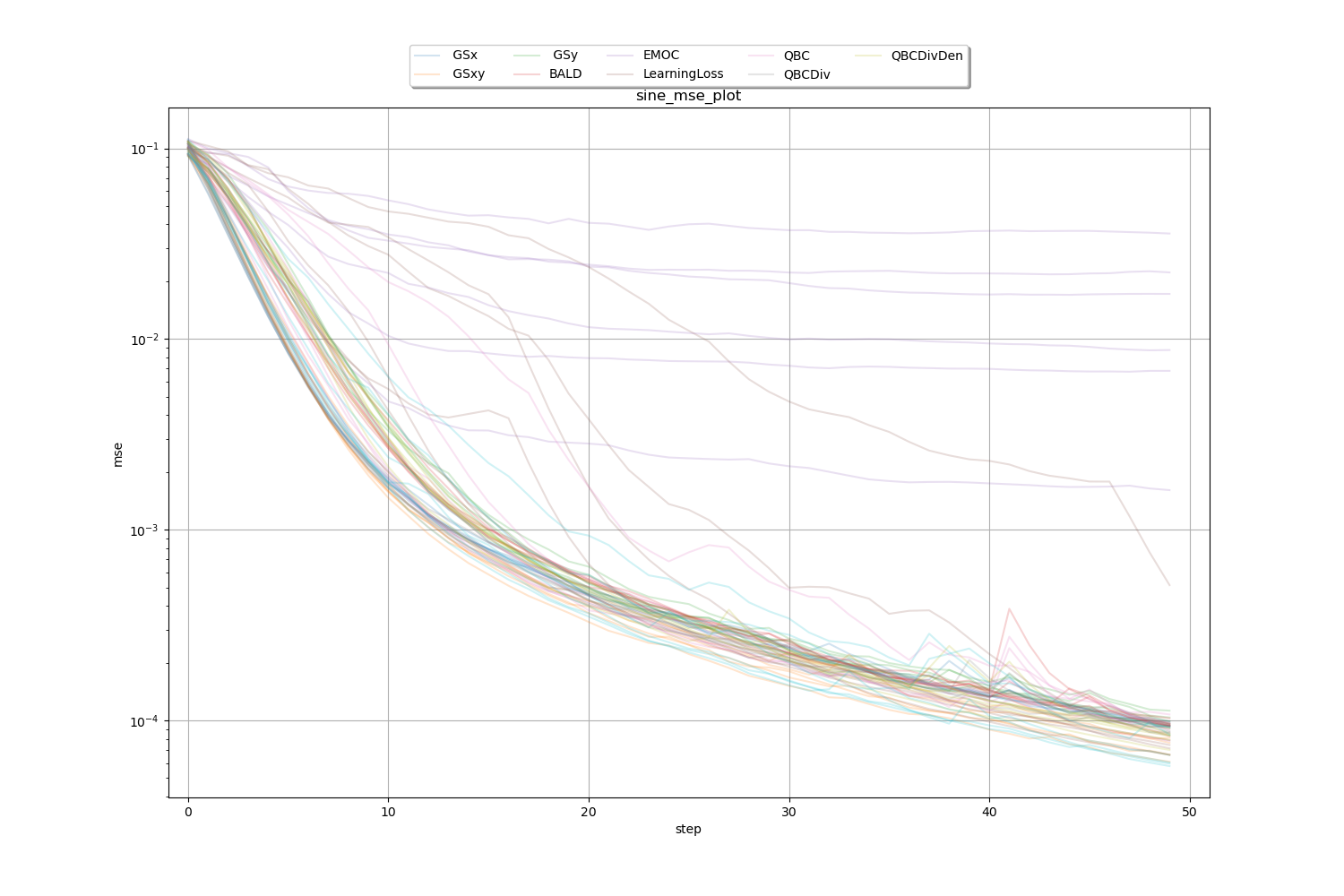
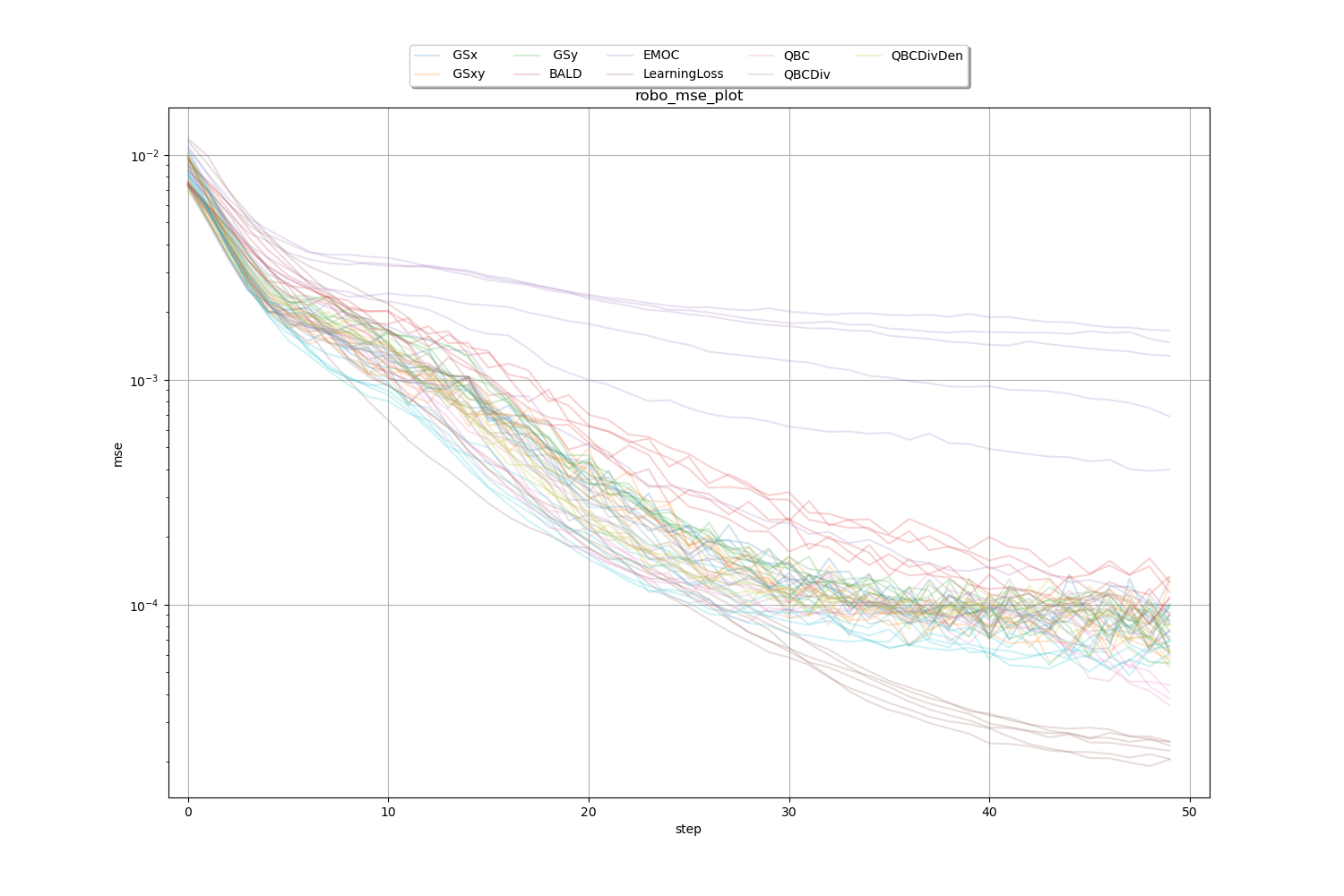
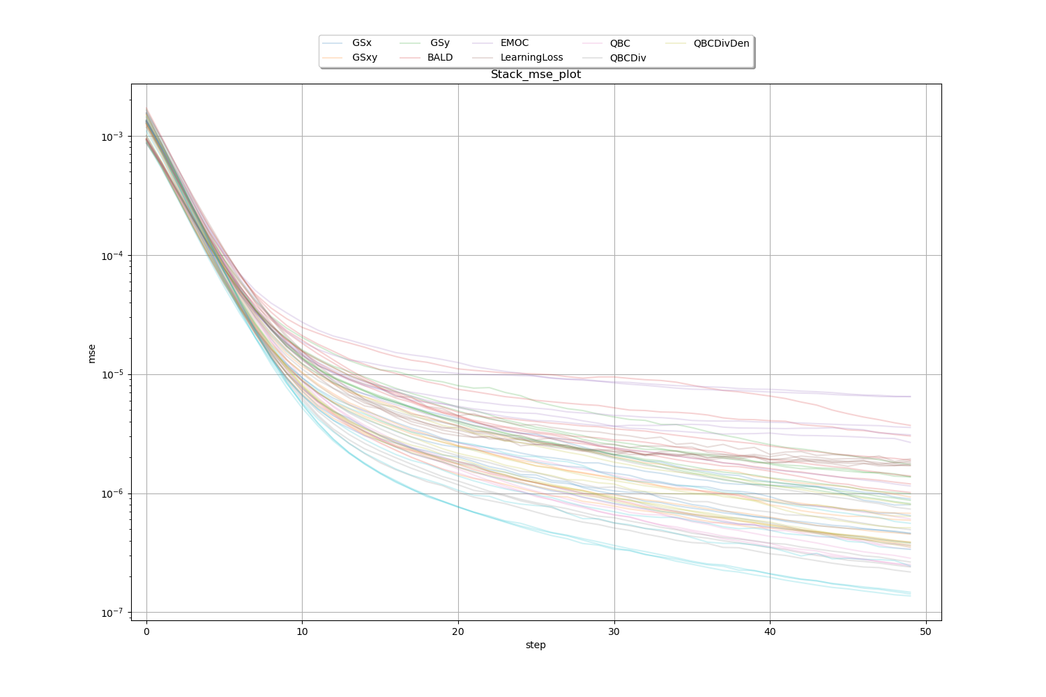
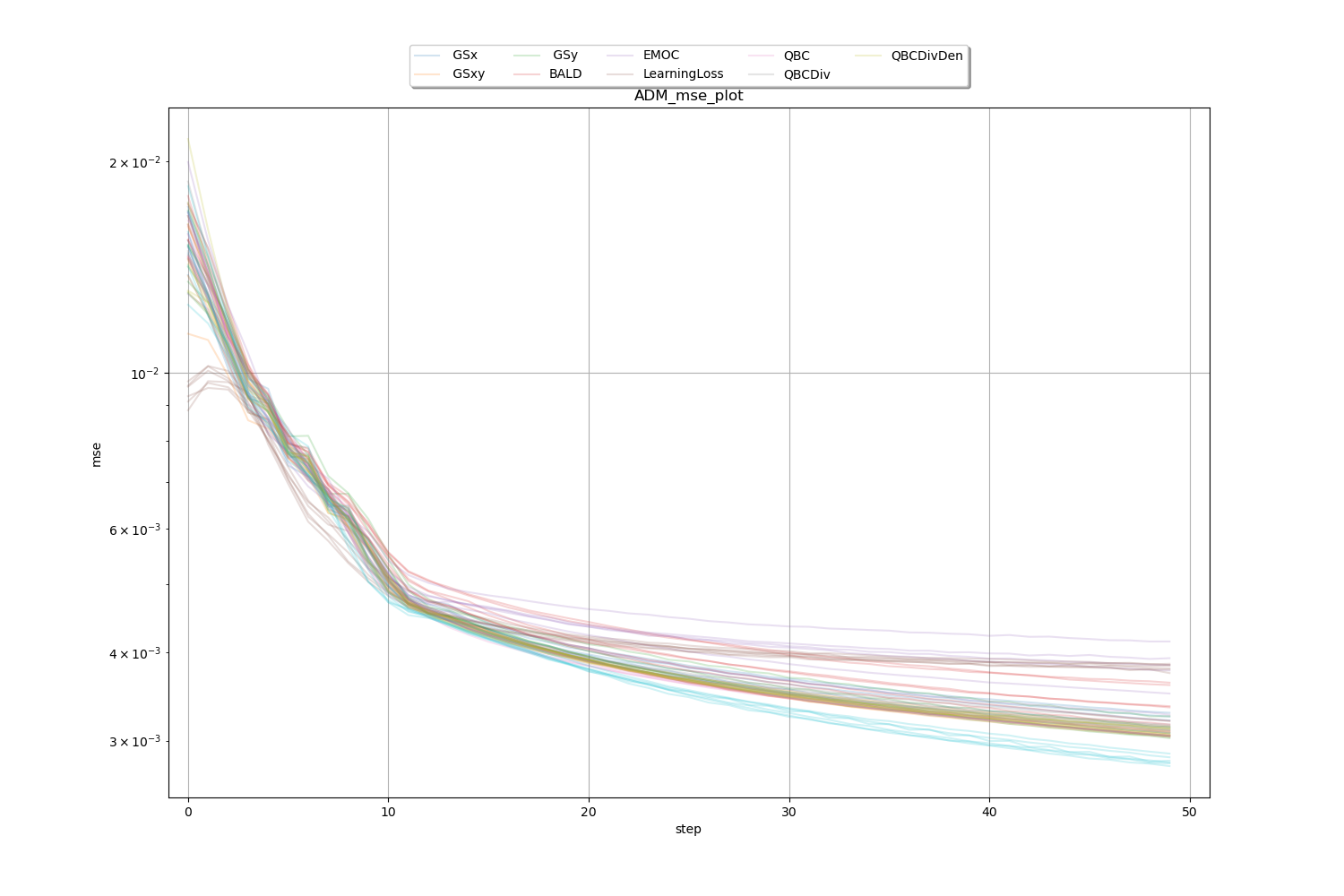
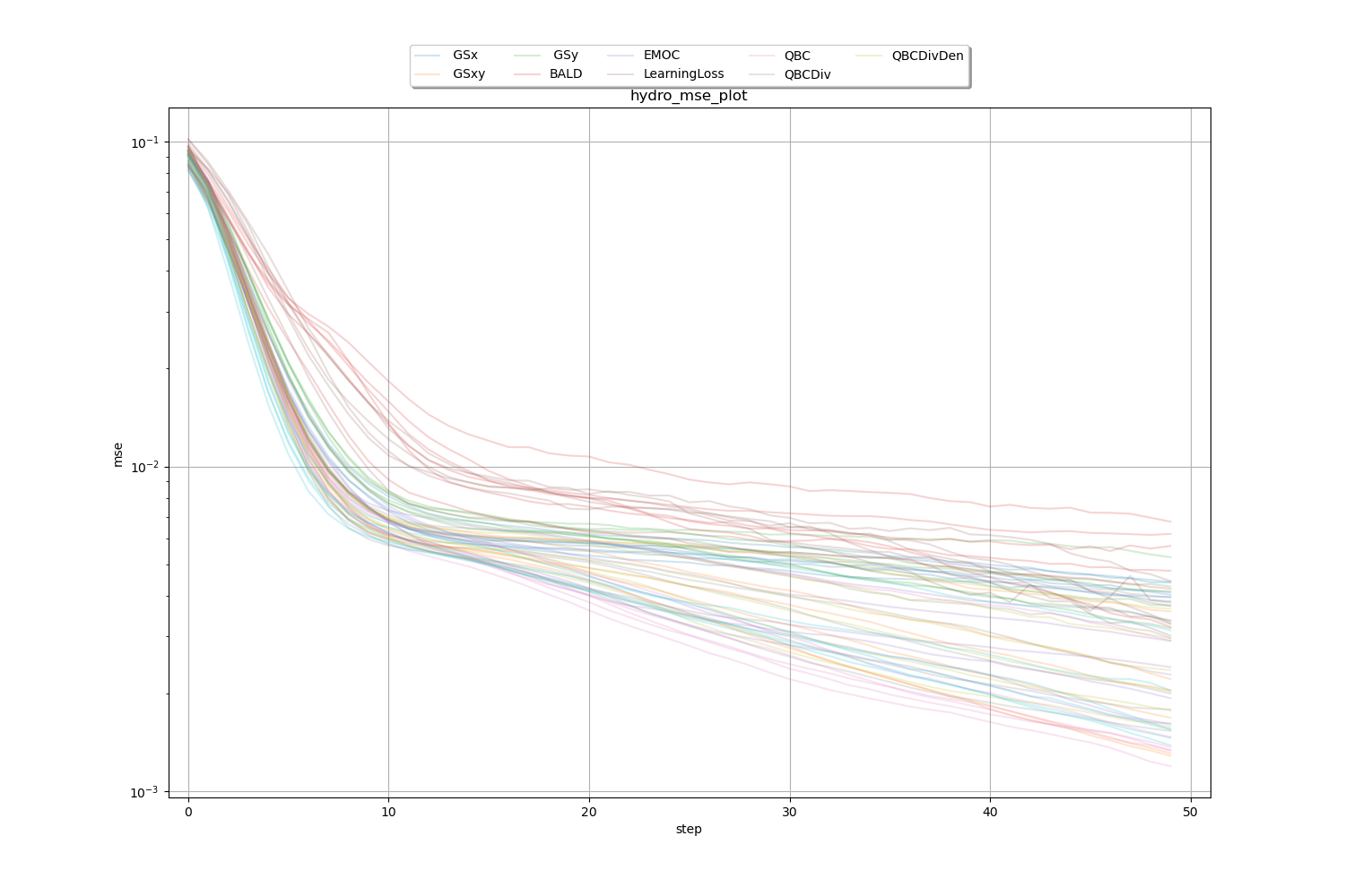
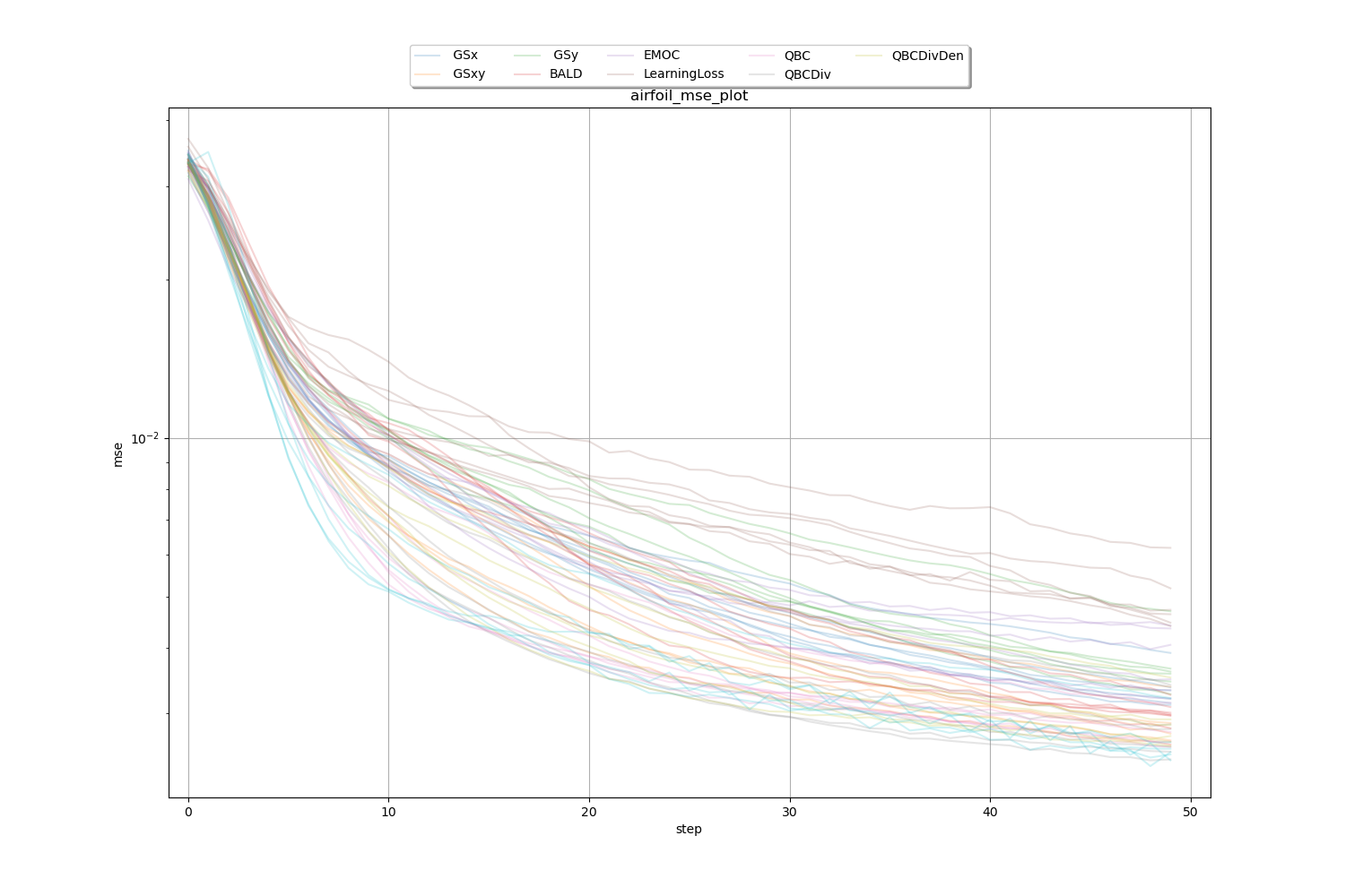
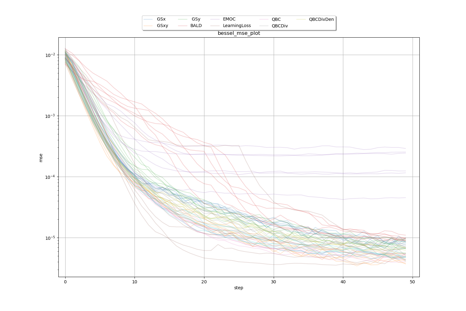
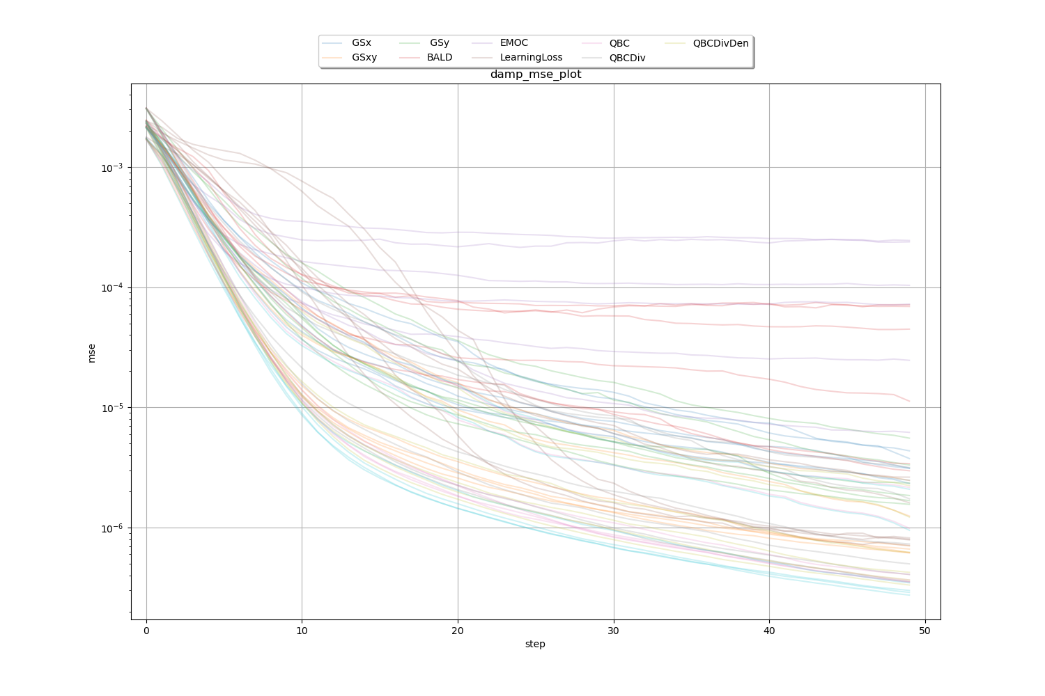
E.3 MSE vs active learning step plot

We also present the traditional plot of the MSE vs active learning step for reference. For each of the plots below, the MSE are smoothed with a smoothing parameter of 0.5 using the tensorboard smoothing visualizing function [53]. The $x$ labels are from 0 - 49, where 0 measures the end of the first active learning step.

Figure 17: MSE plot for SINE

Figure 18: MSE plot for ROBO

Figure 19: MSE plot for STACK

Figure 20: MSE plot for ADM

Figure 21: MSE plot for HYDR

Figure 22: MSE plot for FOIL

Figure 23: MSE plot for BESS

Figure 24: MSE plot for DAMP

References

- [1] J. Jumper, R. Evans, A. Pritzel, T. Green, M. Figurnov, O. Ronneberger, K. Tunyasuvunakool, R. Bates, A. Žídek, A. Potapenko, et al., “Highly accurate protein structure prediction with alphafold,” Nature, vol. 596, no. 7873, pp. 583–589, 2021.
- [2] D. Rolnick, P. L. Donti, L. H. Kaack, K. Kochanski, A. Lacoste, K. Sankaran, A. S. Ross, N. Milojevic-Dupont, N. Jaques, A. Waldman-Brown, et al., “Tackling climate change with machine learning,” arXiv preprint arXiv:1906.05433, 2019.
- [3] A. Lavin, H. Zenil, B. Paige, D. Krakauer, J. Gottschlich, T. Mattson, A. Anandkumar, S. Choudry, K. Rocki, A. G. Baydin, et al., “Simulation intelligence: Towards a new generation of scientific methods,” arXiv preprint arXiv:2112.03235, 2021.
- [4] O. Khatib, S. Ren, J. Malof, and W. J. Padilla, “Deep learning the electromagnetic properties of metamaterials—a comprehensive review,” Advanced Functional Materials, vol. 31, no. 31, p. 2101748, 2021.
- [5] K. T. Schütt, M. Gastegger, A. Tkatchenko, K.-R. Müller, and R. J. Maurer, “Unifying machine learning and quantum chemistry with a deep neural network for molecular wavefunctions,” Nature communications, vol. 10, no. 1, pp. 1–10, 2019.
- [6] C. C. Nadell, B. Huang, J. M. Malof, and W. J. Padilla, “Deep learning for accelerated all-dielectric metasurface design,” Optics express, vol. 27, no. 20, pp. 27523–27535, 2019.
- [7] A. Zhavoronkov, Y. A. Ivanenkov, A. Aliper, M. S. Veselov, V. A. Aladinskiy, A. V. Aladinskaya, V. A. Terentiev, D. A. Polykovskiy, M. D. Kuznetsov, A. Asadulaev, et al., “Deep learning enables rapid identification of potent ddr1 kinase inhibitors,” Nature biotechnology, vol. 37, no. 9, pp. 1038–1040, 2019.
- [8] Y. LeCun, Y. Bengio, and G. Hinton, “Deep learning,” nature, vol. 521, no. 7553, pp. 436–444, 2015.
- [9] P. Ren, Y. Xiao, X. Chang, P.-Y. Huang, Z. Li, B. B. Gupta, X. Chen, and X. Wang, “A survey of deep active learning,” ACM Computing Surveys (CSUR), vol. 54, no. 9, pp. 1–40, 2021.
- [10] B. Settles, “Active learning literature survey,” 2009.
- [11] S. Roy, A. Unmesh, and V. P. Namboodiri, “Deep active learning for object detection.,” in BMVC, vol. 362, p. 91, 2018.
- [12] E. Tsymbalov, M. Panov, and A. Shapeev, “Dropout-based active learning for regression,” in International conference on analysis of images, social networks and texts, pp. 247–258, Springer, 2018.
- [13] C. Käding, E. Rodner, A. Freytag, O. Mothes, B. Barz, J. Denzler, and C. Z. AG, “Active learning for regression tasks with expected model output changes.,” in BMVC, p. 103, 2018.
- [14] S. Kee, E. Del Castillo, and G. Runger, “Query-by-committee improvement with diversity and density in batch active learning,” Information Sciences, vol. 454, pp. 401–418, 2018.
- [15] G. B. Huang, M. Mattar, T. Berg, and E. Learned-Miller, “Labeled faces in the wild: A database forstudying face recognition in unconstrained environments,” in Workshop on faces in’Real-Life’Images: detection, alignment, and recognition, 2008.
- [16] X. Zhan, H. Liu, Q. Li, and A. B. Chan, “A comparative survey: Benchmarking for pool-based active learning.,” in IJCAI, pp. 4679–4686, 2021.
- [17] Y. Yang and M. Loog, “A benchmark and comparison of active learning for logistic regression,” Pattern Recognition, vol. 83, pp. 401–415, 2018.
- [18] V. V. Meduri, L. Popa, P. Sen, and M. Sarwat, “A comprehensive benchmark framework for active learning methods in entity matching,” in Proceedings of the 2020 ACM SIGMOD International Conference on Management of Data, pp. 1133–1147, 2020.
- [19] H. Trittenbach, A. Englhardt, and K. Böhm, “An overview and a benchmark of active learning for outlier detection with one-class classifiers,” Expert Systems with Applications, vol. 168, p. 114372, 2021.
- [20] Q. Hu, Y. Guo, M. Cordy, X. Xie, W. Ma, M. Papadakis, and Y. Le Traon, “Towards exploring the limitations of active learning: An empirical study,” in 2021 36th IEEE/ACM International Conference on Automated Software Engineering (ASE), pp. 917–929, IEEE, 2021.
- [21] N. Beck, D. Sivasubramanian, A. Dani, G. Ramakrishnan, and R. Iyer, “Effective evaluation of deep active learning on image classification tasks,” arXiv preprint arXiv:2106.15324, 2021.
- [22] J. O’Neill, S. Jane Delany, and B. MacNamee, “Model-free and model-based active learning for regression,” in Advances in computational intelligence systems, pp. 375–386, Springer, 2017.
- [23] D. Wu, C.-T. Lin, and J. Huang, “Active learning for regression using greedy sampling,” Information Sciences, vol. 474, pp. 90–105, 2019.
- [24] I. Guyon, G. C. Cawley, G. Dror, and V. Lemaire, “Results of the active learning challenge,” in Active Learning and Experimental Design workshop In conjunction with AISTATS 2010, pp. 19–45, JMLR Workshop and Conference Proceedings, 2011.
- [25] B. Settles, Curious machines: Active learning with structured instances. PhD thesis, University of Wisconsin–Madison, 2008.
- [26] W. Cai, Y. Zhang, and J. Zhou, “Maximizing expected model change for active learning in regression,” in 2013 IEEE 13th international conference on data mining, pp. 51–60, IEEE, 2013.
- [27] J. S. Smith, B. Nebgen, N. Lubbers, O. Isayev, and A. E. Roitberg, “Less is more: Sampling chemical space with active learning,” The Journal of chemical physics, vol. 148, no. 24, p. 241733, 2018.
- [28] H. Yu and S. Kim, “Passive sampling for regression,” in 2010 IEEE International Conference on Data Mining, pp. 1151–1156, IEEE, 2010.
- [29] D. Yoo and I. S. Kweon, “Learning loss for active learning,” in Proceedings of the IEEE/CVF conference on computer vision and pattern recognition, pp. 93–102, 2019.
- [30] H. Ranganathan, H. Venkateswara, S. Chakraborty, and S. Panchanathan, “Deep active learning for image regression,” in Deep Learning Applications, pp. 113–135, Springer, 2020.
- [31] C. Käding, E. Rodner, A. Freytag, and J. Denzler, “Active and continuous exploration with deep neural networks and expected model output changes,” arXiv preprint arXiv:1612.06129, 2016.
- [32] W. H. Beluch, T. Genewein, A. Nürnberger, and J. M. Köhler, “The power of ensembles for active learning in image classification,” in Proceedings of the IEEE conference on computer vision and pattern recognition, pp. 9368–9377, 2018.
- [33] R. Burbidge, J. J. Rowland, and R. D. King, “Active learning for regression based on query by committee,” in International conference on intelligent data engineering and automated learning, pp. 209–218, Springer, 2007.
- [34] M. Takamoto, T. Praditia, R. Leiteritz, D. MacKinlay, F. Alesiani, D. Pflüger, and M. Niepert, “Pdebench: An extensive benchmark for scientific machine learning,” in Thirty-sixth Conference on Neural Information Processing Systems Datasets and Benchmarks Track.
- [35] Y. Deng, J. Dong, S. Ren, O. Khatib, M. Soltani, V. Tarokh, W. Padilla, and J. Malof, “Benchmarking data-driven surrogate simulators for artificial electromagnetic materials,” in Thirty-fifth Conference on Neural Information Processing Systems Datasets and Benchmarks Track (Round 2), 2021.
- [36] O. Sener and S. Savarese, “Active learning for convolutional neural networks: A core-set approach,” arXiv preprint arXiv:1708.00489, 2017.
- [37] S. Ren, W. Padilla, and J. Malof, “Benchmarking deep inverse models over time, and the neural-adjoint method,” Advances in Neural Information Processing Systems, vol. 33, pp. 38–48, 2020.
- [38] Y. Chen, J. Zhu, Y. Xie, N. Feng, and Q. H. Liu, “Smart inverse design of graphene-based photonic metamaterials by an adaptive artificial neural network,” Nanoscale, vol. 11, no. 19, pp. 9749–9755, 2019.
- [39] Y. Deng, S. Ren, K. Fan, J. M. Malof, and W. J. Padilla, “Neural-adjoint method for the inverse design of all-dielectric metasurfaces,” Optics Express, vol. 29, no. 5, pp. 7526–7534, 2021.
- [40] D. Dua and C. Graff, “UCI machine learning repository,” 2017.
- [41] T. F. Brooks, D. S. Pope, and M. A. Marcolini, “Airfoil self-noise and prediction,” tech. rep., 1989.
- [42] D. Wu, “Pool-based sequential active learning for regression,” IEEE transactions on neural networks and learning systems, vol. 30, no. 5, pp. 1348–1359, 2018.
- [43] Z. Liu and D. Wu, “Unsupervised pool-based active learning for linear regression,” arXiv preprint arXiv:2001.05028, 2020.
- [44] F. Pedregosa, G. Varoquaux, A. Gramfort, V. Michel, B. Thirion, O. Grisel, M. Blondel, P. Prettenhofer, R. Weiss, V. Dubourg, J. Vanderplas, A. Passos, D. Cournapeau, M. Brucher, M. Perrot, and E. Duchesnay, “Scikit-learn: Machine learning in Python,” Journal of Machine Learning Research, vol. 12, pp. 2825–2830, 2011.
- [45] H. S. Seung, M. Opper, and H. Sompolinsky, “Query by committee,” in Proceedings of the fifth annual workshop on Computational learning theory, pp. 287–294, 1992.
- [46] S. Ren, A. Mahendra, O. Khatib, Y. Deng, W. J. Padilla, and J. M. Malof, “Inverse deep learning methods and benchmarks for artificial electromagnetic material design,” Nanoscale, vol. 14, no. 10, pp. 3958–3969, 2022.
- [47] B. Trabucco, X. Geng, A. Kumar, and S. Levine, “Design-bench: Benchmarks for data-driven offline model-based optimization,” arXiv preprint arXiv:2202.08450, 2022.
- [48] P. Virtanen, R. Gommers, T. E. Oliphant, M. Haberland, T. Reddy, D. Cournapeau, E. Burovski, P. Peterson, W. Weckesser, J. Bright, S. J. van der Walt, M. Brett, J. Wilson, K. J. Millman, N. Mayorov, A. R. J. Nelson, E. Jones, R. Kern, E. Larson, C. J. Carey, İ. Polat, Y. Feng, E. W. Moore, J. VanderPlas, D. Laxalde, J. Perktold, R. Cimrman, I. Henriksen, E. A. Quintero, C. R. Harris, A. M. Archibald, A. H. Ribeiro, F. Pedregosa, P. van Mulbregt, and SciPy 1.0 Contributors, “SciPy 1.0: Fundamental Algorithms for Scientific Computing in Python,” Nature Methods, vol. 17, pp. 261–272, 2020.
- [49] A. K. McCallumzy and K. Nigamy, “Employing em and pool-based active learning for text classification,” in Proc. International Conference on Machine Learning (ICML), pp. 359–367, Citeseer, 1998.
- [50] J. E. Santos, M. Mehana, H. Wu, M. Prodanovic, Q. Kang, N. Lubbers, H. Viswanathan, and M. J. Pyrcz, “Modeling nanoconfinement effects using active learning,” The Journal of Physical Chemistry C, vol. 124, no. 40, pp. 22200–22211, 2020.
- [51] Y. Tan, L. Yang, Q. Hu, and Z. Du, “Batch mode active learning for semantic segmentation based on multi-clue sample selection,” in Proceedings of the 28th ACM International Conference on Information and Knowledge Management, pp. 831–840, 2019.
- [52] A. Paszke, S. Gross, F. Massa, A. Lerer, J. Bradbury, G. Chanan, T. Killeen, Z. Lin, N. Gimelshein, L. Antiga, A. Desmaison, A. Kopf, E. Yang, Z. DeVito, M. Raison, A. Tejani, S. Chilamkurthy, B. Steiner, L. Fang, J. Bai, and S. Chintala, “Pytorch: An imperative style, high-performance deep learning library,” in Advances in Neural Information Processing Systems 32, pp. 8024–8035, Curran Associates, Inc., 2019.
- [53] M. Abadi, A. Agarwal, P. Barham, E. Brevdo, Z. Chen, C. Citro, G. S. Corrado, A. Davis, J. Dean, M. Devin, S. Ghemawat, I. Goodfellow, A. Harp, G. Irving, M. Isard, Y. Jia, R. Jozefowicz, L. Kaiser, M. Kudlur, J. Levenberg, D. Mané, R. Monga, S. Moore, D. Murray, C. Olah, M. Schuster, J. Shlens, B. Steiner, I. Sutskever, K. Talwar, P. Tucker, V. Vanhoucke, V. Vasudevan, F. Viégas, O. Vinyals, P. Warden, M. Wattenberg, M. Wicke, Y. Yu, and X. Zheng, “TensorFlow: Large-scale machine learning on heterogeneous systems,” 2015. Software available from tensorflow.org.