Abstract

We show that, unlike vacuum General Relativity, Einstein-scalar theories allow balanced static, neutral, asymptotically flat, double-black hole solutions, for scalar field models minimally coupled to gravity, with appropriate self-interactions. These are scalar hairy versions of the double-Schwarzschild (or Bach-Weyl) solution, but regular on and outside the two (topologically spherical) horizons. The balancing repulsive force is provided by the scalar field. An explicit illustration is presented, using a Weyl-type construction adapted to numerical solutions, requiring no partial linearisation, or integrability structure, of the Einstein-scalar equations. Fixing the couplings of the model, the balanced configurations form a one-parameter family of solutions, labelled by the proper distance between the black holes.

1 Introduction

A remarkable solution of “vacuum” General Relativity (GR) is the Bach-Weyl (BW) or double-Schwarzschild metric, describing two static, neutral black holes (BHs) placed at some non-zero distance, in a four dimensional, asymptotically flat spacetime [1]. The gravitational attraction between the BHs is unbalanced; as a result, conical singularities along the symmetry axis are mandated by the field equations [2]. Despite such naked singularities, this solution has a well defined gravitational action. Moreover, the Bekenstein-Hawking area law still holds when using standard Euclidean gravity thermodynamical arguments [3].

The precise location of the conical singularity of the BW solution is a matter of choice. It can either be chosen in between the two BHs - in which case it is interpreted as a strut - or connecting either BH to infinity - in which case it is interpreted as two strings. In order for the spacetime to be asymptotically flat, without any conical singularities at spatial infinity, one often takes the former viewpoint. Then, the strut energy is interpreted as the interaction energy between the BHs, while its pressure prevents the gravitational collapse of the system [4].

On the one hand, the BW solution can be generalised within “vacuum” GR in different ways. One way is to introduce $N$ (instead of 2) colinear, neutral, static BHs, leading to the Israel-Kahn solution [5]. However, this does not solve the need for a conical singularity, except in the $N\rightarrow\infty$ limit [6], which has a natural interpretation as a BH in a compactified spacetime, rather than an asymptotically flat configuration. Another way is to place the BW solution in an appropriate external gravitational field [7, 8]. Such solution ceases, again, to be asymptotically flat; in fact it is plagued by naked curvature singularities at spatial infinity. A final way is to make the BHs spin. The double-Kerr solution can be constructed via elaborate solution generating techniques, such as the inverse scattering method [9]. For co-rotating BHs, with aligned spins, the spin-spin interaction is repulsive [10], introducing a plausible balancing effect. It turns out, however, that this extra interaction cannot balance the system, for objects covered by an event horizon - see $e.g.$ [11]. A physical explanation has been put forward in [12].

On the other hand, the BW solution can be generalised within electrovacuum GR to yield balanced, asymptotically flat configurations. This involves making the BHs extremal, $i.e.$ with their maximal charge to mass ratio. The corresponding balanced BHs fall into the Majumdar-Papapetrou class of metrics [13, 14], describing $N$ extremal Reissner-Nordström BHs in equilibrium [15], which are regular on and outside the event horizon and asymptotically flat. Such solutions can also be generalized to Einstein-Maxwell dilatonic theories - see $e.g.$ [16, 17, 18]. There are also non-asymptotically flat charged BHs in equilibrium, when immersed in a Melvin-type universe [19] or in a de Sitter Universe [20]; in the latter case the BHs are co-moving with the cosmological expansion.

To the best of our knowledge, no static, electro-magnetically neutral, asymptotically flat BHs in equilibrium are known in four spacetime dimensions. There is no reason, however, to expect this to be a fundamental feature of relativistic gravity. Conceptually, the electromagnetic repulsive interaction that allows balance in some of the aforementioned solutions could, in principle, be replaced by another repulsive interaction, namely scalar. Technically, however, one faces important obstacles.

For solutions akin to the Majumdar-Papapetrou solution (multi-BHs experiencing a “no-force” condition), common in supergravity theories (see $e.g.$ [23]), under an appropriate ansatz one observes a full linearization of the Einstein-matter equations. This allows a superposition principle that corresponds to adding multiple BHs and it is intimately connected with supersymmetry [24, 25]. For solutions akin to the double-Schwarzschild metric, under an appropriate ansatz - corresponding to the Weyl formalism [26], one observes a partial linearization of the full Einstein equations. This still allows a superposition principle for a specific metric function, which in effect corresponds to adding multiple BHs, with the remaining metric functions obeying non-linear equations, which can, nonetheless, be straighforwardly solved once the linear metric function function is known. The Weyl formalism comes with an intuitive diagramatic construction - the rod structure (see $e.g.$ [27, 28]) - that permits constructing new solutions. The static Weyl solutions constructed in this way, moreover, serve as natural seeds for the inverse scattering technique [29], that can add rotation (and other properties, such as NUT charges) to the solutions.

For scalar fields with canonical kinetic terms, minimally coupled to Einstein’s theory, possibly with some self-interacting potentials – hereafter Einstein-scalar theories –, the Weyl construction has not been made to work, except in the case of free, massless scalar fields [30, 31]. In the absence of a methodology to obtain exact multi-BH solutions, one may approach such configurations numerically, as solutions of partial differential equations (PDEs) with suitable boundary conditions. This paper aims at proposing a general framework for the study of static multi-BH systems with matter fields, numerically. As an application, we shall report solutions describing two balanced BHs (hereafter dubbed 2BHs) in a specific Einstein-scalar theory.

The construction we propose is, in principle, more general than scalar matter models. The choice of a scalar field for the matter content is mainly motivated by its simplicity, both technical and conceptual. Simultaneously, the influential theorem by Bekenstein [32] forbidding the existence of (single) BHs with scalar hair can be circumvented in different ways [33]. A simple way is to allow a scalar field potential which is not strictly positive, such that the energy conditions assumed by the theorem are violated [33]. Such scalar fields can provide an extra repulsive interaction, balancing a non-trivial scalar field profile outside the horizon. (Single) BHs with scalar hair are allowed by this mechanism, $e.g.$ [34, 35, 36, 37].

One may thus anticipate the same mechanism to work for the 2BHs case as well. A scalar field potential which can take negative values in the region between the horizons, moreover, could provide the extra (repulsive) interaction to balance two neutral static BHs, curing the conical singularity of the BW solution. Indeed, this is confirmed by the results in this work, where we present numerical evidence for the existence of balanced 2BHs solutions in this setting. A central point in our approach is that the rod structure of the BW solution can be used also for such Einstein-matter configurations, in particular for the 2BHs system with scalar hair, even though the partial linearization of the Einstein-scalar equations and the vacuum Newtonian interpretation of the rods cease to be valid. The application given in this work will focus on 2BH systems in thermal equilibrium, $i.e.$ with two identical BHs placed at some distance.

This paper is organized as follows. In Section 2 we present the Einstein-scalar model we shall work with. The canonical Weyl construction is attempted with this model, to observe the known obstructions. Then, we specialize to vacuum to discuss the Schwarzschild, double-Schwarzschild (or BW) solutions and the rod structure. In Section 3 we present a Weyl-type construction adapted to numerics, readdressing the rod structure, discussing the boundary conditions and the single BH limit. In Section 4 we specialize to a potential that allows BHs to have scalar hair and thus that may allow such hair to balance two BHs. We then report the results for such 2BHs balanced system. Some final remarks close this paper, which also contains three appendices with technical details, together with a numerical construction of the double-Reissner-Nordström solution (2RNBHs), as a test of the proposed numerical scheme.

2 Einstein-scalar models and the vacuum Weyl construction

2.1 The action and equations

We consider the Einstein-scalar model described by the following action

$$\mathcal{S}=\frac{1}{4\pi}\int d^{4}x\sqrt{-g}\left[\frac{R}{4G}-\frac{1}{2}g^{\alpha\beta}\left(\Phi_{,\,\alpha}^{*}\Phi_{,\,\beta}+\Phi_{,\,\alpha}^{*}\Phi_{,\,\beta}\right)-U(\left|\Phi\right|)\right]~{},$$ (2.1)

where $G$ is the gravitational constant, $R$ is the Ricci scalar associated with the spacetime metric $g_{\alpha\beta}$, which has determinant $g$, $\Phi$ is a complex scalar field with ^∗ denoting complex conjugation and $U(|\Phi|)$ denotes the scalar potential. The scalar field mass is defined by $\mu^{2}\equiv(d^{2}U/d|\Phi|^{2})\big{|}_{\Phi=0}$.

The Einstein–scalar field equations, obtained by varying (2.1) with respect to the metric and scalar field are, respectively,

$$E_{\alpha\beta}\equiv R_{\alpha\beta}-\frac{1}{2}g_{\alpha\beta}R-2GT_{\alpha\beta}=0\ ,\qquad~{}~{}~{}\nabla_{\alpha}\nabla^{\alpha}\Phi=\frac{dU}{d\left|\Phi\right|}\ ,$$ (2.2)

where $T_{\alpha\beta}$ is the energy-momentum tensor of the scalar field

$$T_{\alpha\beta}=\partial_{\alpha}\Phi^{*}\partial_{\beta}\Phi+\partial_{\beta}\Phi^{*}\partial_{\alpha}\Phi-g_{\alpha\beta}\left[\frac{1}{2}g^{\gamma\delta}(\partial_{\gamma}\Phi^{*}\partial_{\delta}\Phi+\partial_{\delta}\Phi^{*}\partial_{\gamma}\Phi)+U(\left|\Phi\right|)\right]\ .$$ (2.3)

2.2 Canonical Weyl-coordinates

The configurations we shall consider herein are static and axially symmetric, admitting two orthogonal, commuting, non-null Killing Vector Fields (KVFs). In what follows we take their line element written in coordinates adapted these symmetries, $(t,\rho,z,\varphi)$, such that $\partial_{t}$ and $\partial_{\varphi}$ are KVFs; it reads

$$ds^{2}=-e^{2\mathcal{U}(\rho,z)}dt^{2}+e^{-2\mathcal{U}(\rho,z)}\left[e^{2\mathcal{K}(\rho,z)}(d\rho^{2}+dz^{2})+e^{2\mathcal{C}(\rho,z)}\rho^{2}d\varphi^{2}\right]\ ,$$ (2.4)

thus introducing three unknown functions $\mathcal{U}$, $\mathcal{K}$ and $\mathcal{C}$ of the non-Killing coordinates $(\rho,z)$, where $0\leqslant\rho<\infty,$ $-\infty<z<\infty$ and $0\leqslant\varphi<2\pi$. For the scalar field $\Phi$, we take a generic ansatz

$$\Phi=\phi(\rho,z)e^{im\varphi}\ ,$$ (2.5)

with $\phi$ a real function – the scalar field amplitude –, and $m\in\mathbb{Z}$.

Appropriate combinations of the Einstein equations, $E_{t}^{t}=0$, $E_{\rho}^{\rho}+E_{z}^{z}=0$ and $E_{\varphi}^{\varphi}=0$, yield the following set of equations for the functions $\mathcal{U}$, $\mathcal{K}$, and $\mathcal{C}$,

$$\Delta\mathcal{U}+(\nabla\mathcal{U})\cdot(\nabla\mathcal{C})=-2Ge^{2(\mathcal{K}-\mathcal{U})}U(\phi)\ ,$$

$$\Delta\mathcal{K}-\frac{\mathcal{K}_{,\rho}}{\rho}+(\nabla\mathcal{U})^{2}=-2G\left[(\nabla\phi)^{2}+e^{2(\mathcal{K}-\mathcal{U})}U(\phi)-\frac{e^{2(\mathcal{K}-\mathcal{C})}m^{2}\phi^{2}}{\rho^{2}}\right]\ ,$$

$$\Delta\mathcal{C}+\frac{\mathcal{C}_{,\rho}}{\rho}+(\nabla\mathcal{C})^{2}=-4Ge^{2(\mathcal{K}-\mathcal{U})}\left[U(\phi)+\frac{e^{2(\mathcal{U}-\mathcal{C})}m^{2}\phi^{2}}{\rho^{2}}\right]\ .$$ (2.6)

The equation for the scalar field amplitude $\phi$ is

$$\Delta\phi+(\nabla\mathcal{C})\cdot(\nabla\phi)=\frac{1}{2}e^{2(\mathcal{K}-\mathcal{U})}\frac{dU(\phi)}{d\phi}+\frac{e^{2(\mathcal{K}-\mathcal{C})}m^{2}\phi}{\rho^{2}}\ ,$$ (2.7)

We have defined, acting on arbitrary functions $\mathcal{F}(\rho,z)$ and $\mathcal{G}(\rho,z)$,

$$(\nabla\mathcal{F})\cdot(\nabla\mathcal{G})\equiv\mathcal{F}_{,\rho}\mathcal{G}_{,\rho}+\mathcal{F}_{,z}\mathcal{G}_{,z}\ ,\qquad\Delta\mathcal{F}\equiv\mathcal{F}_{,\rho\rho}+\mathcal{F}_{,zz}+\frac{1}{\rho}\mathcal{F}_{,\rho}\ .$$ (2.8)

These operators are the covariant operators on an auxiliary Euclidean 3-space in standard cylindrical coordinates, $ds^{2}_{\rm auxiliary}=d\rho^{2}+\rho^{2}d\varphi^{2}+dz^{2}$.

The remaining Einstein equations $E_{\rho}^{z}=0,~{}E_{\rho}^{\rho}-E_{z}^{z}=0$ yield two constraints,

$$\mathcal{C}_{,\rho\rho}+\frac{2\mathcal{C}_{,\rho}}{\rho}-\mathcal{C}_{,zz}+2(\mathcal{U}_{,\rho}^{2}-\mathcal{U}_{,z}^{2})+\mathcal{C}_{,\rho}^{2}-\mathcal{C}_{,z}^{2}-2(\mathcal{C}_{,\rho}\mathcal{K}_{,\rho}-\mathcal{C}_{,z}\mathcal{K}_{,z})-\frac{2\mathcal{K}_{,\rho}}{\rho}+4G(\phi_{,\rho}^{2}-\phi_{,z}^{2})=0\ ,$$

$$\mathcal{C}_{,\rho z}+\mathcal{C}_{,\rho}\mathcal{C}_{,z}+2\mathcal{U}_{,\rho}\mathcal{U}_{,z}-\mathcal{C}_{,\rho}\mathcal{K}_{,z}-\mathcal{K}_{,\rho}\mathcal{C}_{,z}+\frac{\mathcal{C}_{,z}}{\rho}-\frac{\mathcal{K}_{,z}}{\rho}+4G\phi_{,\rho}\phi_{,z}=0\ .$$ (2.9)

Following [38], we note that setting $E^{t}_{t}=E^{\varphi}_{\varphi}=E^{\rho}_{\rho}+E^{z}_{z}=0$ in $\nabla_{\alpha}E^{\alpha\rho}=0$ and $\nabla_{\alpha}E^{\alpha z}=0$, we obtain a set of Cauchy-Riemann relations. Thus the weighted constraints satisfy Laplace equations, and the constraints are fulfilled, when one of them is satisfied on the boundary and the other at a single point [38].

2.3 Scalar-vacuum

In the absence of a scalar potential, $i.e.$ $U(\phi)=0$, and for a real scalar ($m=0$), the third equation in (2.6) allows us to take $\mathcal{C}=0$. The problem then has only three unknown functions, $\mathcal{U}$, $\mathcal{K}$, and $\phi$. Two of them obey linear equations. Indeed, the first equation in (2.6) and the scalar equation become Laplace-type equations

$$\Delta\mathcal{U}=0\ ,\qquad\Delta\phi=0\ .$$ (2.10)

This is the aforementioned partial linearization of the Einstein equations. It is easy to see from (2.6) that this linearization is lost for $m\neq 0$ or in the presence of a potential $U(\phi)$, which leads to a nuisance (from the viewpoint of the Weyl construction) source term. The source term is, however, absent for a free, massless real scalar. The Weyl construction has in fact been explored in that case [30, 31].

Instead of determining the remaining function $\mathcal{K}(\rho,z)$ from the second eq. in (2.6), it can be determined from the two constraint equations (2.9), which reduce to

$$\mathcal{K}_{,\rho}=\rho(\mathcal{U}_{,\rho}^{2}-\mathcal{U}_{,z}^{2})+4G\rho(\phi_{,\rho}^{2}-\phi_{,z}^{2})\ ,\qquad \mathcal{K}_{,z}=2\rho\mathcal{U}_{,\rho}\mathcal{U}_{,z}+4G\rho\phi_{,\rho}\phi_{,z}\ .$$ (2.11)

Thus, once $\mathcal{U},\phi$ are determined by solving the linear equations (2.10), then $\mathcal{K}$ is determined by solving two line integrals from (2.11). With what concerns BHs, this scalar-vacuum Weyl construction has not been rewarding, as in scalar vacuum BH hair is forbidden [32, 33]. As such, let us focus on the particular case of vacuum ($\phi=0$).

2.4 Vacuum: Schwarzschild and rod-structure

Setting $\phi=0$ in (2.10) and (2.11), the simplest solution has $\mathcal{U}=0=\mathcal{K}$, which is Minkowski spacetime. We are now interested in asymptotically Minkowski solutions.

The Schwarzschild BH with mass $M$ appears in this Weyl construction as the Newtonian potential $\mathcal{U}$ of an infinitely thin rod of length $2M$ along the $z$-axis. Placing this rod symmetrically w.r.t. $z=0$ between $z=-M$ and $z=M$, this means that

$$e^{2\mathcal{U}}=\frac{r_{+}+r_{-}-2M}{r_{+}+r_{-}+2M}\ ,\qquad r_{\pm}=\sqrt{\rho^{2}+\left(z\pm M\right)^{2}}\ .$$ (2.12)

Additionally, from (2.11)

$$e^{2\mathcal{K}}=\frac{(r_{+}+r_{-})^{2}-(2M)^{2}}{4r_{+}r_{-}}\ .$$ (2.13)

The standard Schwarzschild coordinates $(t,r,\theta,\varphi)$ can be recovered from the transformation $(\rho,z)\rightarrow(r,\theta)$ via

$$\rho=\sqrt{r^{2}-2Mr}\sin\theta\ ,\qquad z=(r-M)\cos\theta\ .$$ (2.14)

A large class of solutions in Weyl coordinates are characterized by the boundary conditions on the $z-$axis, known as the rod-structure. That is, the $z-$axis is divided into $N$ intervals (called rods of the solution), $[-\infty,z_{1}]$, $[z_{1},z_{2}]$,$\dots$, $[z_{N-1},\infty]$. A necessary condition for a regular solution is that only one of the functions $g_{tt}(0,z)$ or $g_{\varphi\varphi}(0,z)$ becomes zero for a given rod (except for isolated points between the intervals).

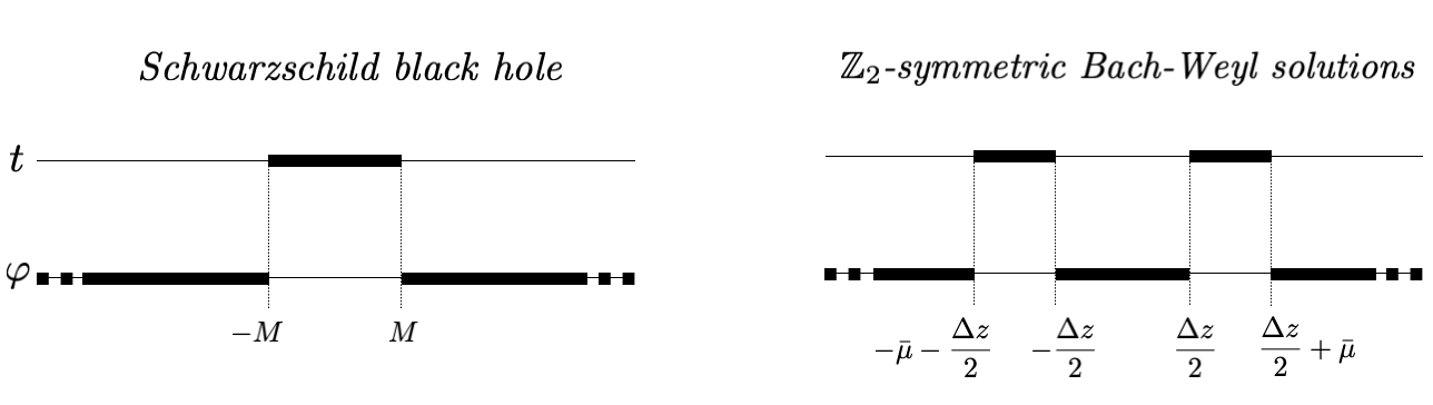
Figure 1: Rod structure, encoding the boundary conditions at $\rho=0$ along the $z$ axis, for the Schwarzschild solution (left) and $\mathbb{Z}_{2}$-symmetric BW solution (right).

The rods are timelike or spacelike:

• Event horizons are described by timelike rods. They are sets of fixed points of the $\partial_{t}$ KVF with $g_{tt}(0,z)=0$ and

  $$\lim_{\rho\to 0}\frac{g_{tt}(\rho,z)}{\rho^{2}}<0\ .$$ (2.15)

• The symmetry axes are described by spacelike rods. They are sets of fixed points of the $\partial_{\varphi}$ KVK, with $g_{\varphi\varphi}(0,z)=0$ and

  $$\lim_{\rho\to 0}\frac{g_{\varphi\varphi}(\rho,z)}{\rho^{2}}>0\ .$$ (2.16)

Fig. 1 (left panel) exhibits the rod structure of the Schwarzschild solution.

2.5 Vacuum: $\mathbb{Z}_{2}$-symmetric Bach-Weyl

The rod structure allows an intuitive, diagramatic-based reconstruction of the metric. For instance, one can easily imagine the rod structure of the double-Schwarzschild (or BW) solution - Fig. 1 (right panel). Choosing the location of the horizons $\mathbb{Z}_{2}$-symmetric with respect to $z=0$, both at $\rho=0$, with the “lower” one at $-\Delta z/2-\bar{\mu}\leqslant z\leqslant-\Delta z/2$ and the “upper” one at $\Delta z/2\leqslant z\leqslant\Delta z/2+\bar{\mu}$, the $g_{tt}$ metric function is defined by the corresponding Newtonian potential, which reads:

$$e^{2\mathcal{U}}=\frac{(r_{1}+r_{2}-\bar{\mu})}{(r_{1}+r_{2}+\bar{\mu})}\frac{(r_{3}+r_{4}-\bar{\mu})}{(r_{3}+r_{4}+\bar{\mu})}\ ,$$ (2.17)

where

$$r_{1}=\sqrt{\rho^{2}+\left(z-\frac{\Delta z}{2}-\bar{\mu}\right)^{2}},~{}~{}r_{2}=\sqrt{\rho^{2}+\left(z-\frac{\Delta z}{2}\right)^{2}},~{}~{}$$ (2.18)

$$r_{3}=\sqrt{\rho^{2}+\left(z+\frac{\Delta z}{2}\right)^{2}},~{}~{}r_{4}=\sqrt{\rho^{2}+\left(z+\frac{\Delta z}{2}+\bar{\mu}\right)^{2}}.$$

Again, from (2.11)

$$e^{2\mathcal{K}}=\left(\frac{\Delta z}{\Delta z+\bar{\mu}}\right)^{2}\left(\frac{(r_{1}+r_{2})^{2}-\bar{\mu}^{2}}{4r_{1}r_{2}}\right)\left(\frac{(r_{3}+r_{4})^{2}-\bar{\mu}^{2}}{4r_{3}r_{4}}\right)\left(\frac{(\Delta z+\bar{\mu})r_{1}+(\Delta z+2\bar{\mu})r_{2}-\bar{\mu}r_{4}}{\Delta z~{}r_{1}+(\Delta z+\bar{\mu})r_{2}-\bar{\mu}r_{3}}\right)^{2}\ .$$ (2.19)

This 2-parameter solution describes two equal BHs in thermodynamical equilibrium - with the same Hawking temperature and horizon area. The parameter $\bar{\mu}$ is the ADM mass of this spacetime (twice the individual BH masses):

$$M=\bar{\mu}>0\ .$$ (2.20)

The parameter $\Delta z\geqslant 0$ provides the coordinate distance between the two horizons along the $z$ axis.

This system has a deficit angle along the section in between the BHs, $i.e.$ for $-\Delta z/2\leqslant z\leqslant\Delta z/2$, with a strength $\delta$, as defined by the relation (3.10) below, given by:

$$\frac{\delta}{2\pi}=-\frac{\bar{\mu}^{2}}{(\Delta z+2\bar{\mu})\Delta z}<0\ .$$ (2.21)

The proper distance between the BHs is

$$L=\int_{-\Delta z/2}^{\-\Delta z/2}dzf_{1}(0,z)=\Delta z\left(\frac{u+4}{u+2}\right)^{2}E(\bar{m})\ ,~{}~{}~{}{\rm where}~{}~{}u=\frac{2\Delta z}{\bar{\mu}}\ ,~{}~{}\bar{m}=\left(\frac{u}{u+4}\right)^{2}\ ,$$ (2.22)

$E(\bar{m})$ being the complete elliptic integral of the second kind. The event horizon area of each BH and the corresponding Hawking temperature are:

$$A_{H}=4\pi\bar{\mu}^{2}\frac{\Delta z+2\bar{\mu}}{\Delta z+\bar{\mu}}\ ,\qquad T_{H}=\frac{1}{4\pi\bar{\mu}}\frac{\Delta z+\bar{\mu}}{\Delta z+2\bar{\mu}}\ .$$ (2.23)

For $\Delta z=0$ the two BH horizons coalesce, and we are left the (single) Schwarzschild BH in Weyl coordinates. Also, the solution trivializes as $\bar{\mu}\to 0$, a limit which corresponds to flat spacetime.

We remark that the solution above captures already all the basic features of its Israel-Kahn generalization [5], with $N$ horizons placed arbitrarily on a common symmetry axis. However, the $N>2$ metric functions get increasingly more involved, albeit with an underlying common structure.

3 A Weyl-type construction adapted to numerics

3.1 The rod structure and quantities of interest

The Weyl construction does not carry through to generic matter models, as illustrated in the previous section for the Einstein-scalar models with a potential. In this work, however, we argue that the Weyl coordinates in (2.4) together with the rod structure of the vacuum multi-BH solutions can be used to construct physically relevant solutions beyond the simplest theories where the Weyl construction allows a partial linearization of the field equations. A priori, this is not guaranteed, and the validity of the metric ansatz could be proven only a posteriori, after solving the field equations. Of course, the elegant Newtonian interpretation of the rods is lost in the non-(scalar, electro)vacuum case; but a working method allows exploring the physics of the non-linear solutions.

Even though one could hold on to the canonical metric parameterization in the Weyl ansatz (2.4), a numerical implementation, namely the boundary conditions at the horizons, is facilitated by taking the simpler parameterization of the metric functions

$$ds^{2}=-f_{0}(\rho,z)dt^{2}+f_{1}(\rho,z)(d\rho^{2}+dz^{2})+f_{2}(\rho,z)d\varphi^{2}\ ;$$ (3.1)

in other words, we relabel

$$f_{0}(\rho,z)\equiv e^{2\mathcal{U}(\rho,z)}\ ,\qquad f_{1}(\rho,z)\equiv e^{-2\mathcal{U}(\rho,z)+2\mathcal{K}(\rho,z)}\ ,\qquad f_{2}(\rho,z)\equiv\rho^{2}e^{-2\mathcal{U}(\rho,z)+2\mathcal{C}(\rho,z)}\ .$$ (3.2)

For completeness, the field equations in terms of this parameterization are given in Appendix A. With this parameterization the following expressions of the metric functions and scalar field near the $z-$axis are compatible with the Einstein-scalar field equations:

$$f_{i}(\rho,z)=f_{i0}(z)+\rho^{2}f_{i2}(z)+\dots\ ,\qquad\phi(\rho,z)=\phi_{0}(z)+\rho^{2}\phi_{2}(z)+\dots\ ,$$ (3.3)

where the functions $f_{i0}(z)$, $f_{i2}(z)$ (with $i=0,1,2$) and $\phi_{0}(z)$, $\phi_{2}(z)$ satisfy a complicated set of nonlinear second order ordinary differential equations.

Our main assumption (supported by the results reported below) is that, similarly to the vacuum case, the $z-$axis is divided into $N$ intervals: the rods of the solution. Moreover, we assume that, except for isolated points between the rods, only one of the functions $f_{0}(0,z)$ or $f_{2}(0,z)$ becomes zero for a given rod, while the remaining functions stay finite at $\rho=0$, in general. Also, one imposes the condition that the union of the $N$ intervals covers the entire $z$-range. There are again timelike and spacelike rods, which we now discuss separately.

A finite timelike rod corresponds to an event horizon, which we assume is located for $z_{H_{1}}\leqslant z\leqslant z_{H_{2}}$. Therein, one can further specify the generic expansion (3.3) to have $f_{00}(z)=0$, such that

$$f_{0}(\rho,z)=\rho^{2}f_{02}(z)+\rho^{4}f_{04}(z)+\dots\ ,$$ (3.4)

with $\lim_{\rho\to 0}\rho^{2}f_{1}/f_{0}=$const., as implied by the constraint equation $E_{\rho}^{z}=0$. The horizon metric is given by

$$d\sigma^{2}_{H}=f_{1}(0,z)dz^{2}+f_{2}(0,z)d\varphi^{2}\ .$$ (3.5)

Two quantities associated with an event horizon are the event horizon area $A_{H}$ and the Hawking temperature $T_{H}$; they read

$$A_{H}=2\pi\int_{z_{H_{1}}}^{z_{H_{2}}}dz\sqrt{f_{1}(0,z)f_{2}(0,z)}\ ,\qquad T_{H}=\frac{1}{2\pi}\lim_{\rho\to 0}\sqrt{\frac{f_{0}(\rho,z)}{\rho^{2}f_{1}(\rho,z)}}\ .$$ (3.6)

The horizon has a spherical topology (despite the possible presence of conical singularities). A suggestive way to graphically represent its shape – which is generically very different from a round 2-sphere – is to define an effective horizon radius ${\rm R}$ [4], by introducing an angular variable $z=z(\theta)$, such that the horizon metric (3.5) becomes

$$d\sigma^{2}={\rm R}^{2}(\theta)(d\theta^{2}+\sin^{2}\theta d\varphi^{2})\ ,\qquad{\rm with}~{}~{}{\rm R}=\frac{\sqrt{f_{2}(0,z)}}{\sin\theta}\ ,$$ (3.7)

where

$$\theta(z)=2\arctan\left[C{\rm exp}\left({\int_{z_{H1}}^{z}dx\sqrt{\frac{f_{1}(0,x)}{f_{2}(0,x)}}}\right)\right]\ .$$ (3.8)

As with the vacuum BW solution [4], the constant $C$ is fixed by by requiring the horizon to be regular at the pole opposite to the other hole. Alternatively, one can use the standard approach developed by Smarr for the Kerr BH [46], and consider an isometric embedding of the horizon geometry (3.5) in $\mathbb{E}^{3}$.

Let us now consider the case of a generic spacelike $\varphi-$rod, for $z_{S_{1}}\leqslant z\leqslant z_{S_{2}}$. Therein, one can further specify the generic expansion (3.3) to have $f_{20}(z)=0$, such that, as $\rho\to 0$:

$$f_{2}(\rho,z)=\rho^{2}f_{22}(z)+\rho^{4}f_{24}(z)+\dots\ .$$ (3.9)

One important feature here is that the constraint equation $E_{\rho}^{z}=0$ implies the condition $f_{10}(z)/f_{22}(z)=$const., $i.e.$ a well-defined periodicity for the coordinate $\varphi$, albeit not necessarily of $2\pi$. A periodicity different from $2\pi$ leads to the occurrence of a conical singularity. Its strength can be measured by means of the quantity

$$\delta=2\pi\left(1-\lim_{\rho\rightarrow 0}\sqrt{\frac{f_{2}(\rho,z)}{\rho^{2}f_{1}(\rho,z)}}\right)\ .$$ (3.10)

Then $\delta>0$ corresponds to a conical deficit, while $\delta<0$ corresponds to a conical excess. As with the “vacuum” case, a conical deficit can be interpreted as a string stretched along a certain segment of the $z-$axis, while a conical excess is a strut pushing apart the rods connected to that segment. A rescaling of $\varphi$ can be used to eliminate possible conical singularities on a given $\varphi$-rod; but in the generic case, once this is fixed, there remain conical singularities along other $\varphi$-rods. Since we are interested in asymptotically flat solutions, we impose $\delta=0$ for the semi-infinite spacelike rods.

Another quantity of interest is the proper length of a $\varphi$-rod

$$L=\int_{z_{S_{1}}}^{z_{S_{2}}}dz\sqrt{f_{1}(0,z)}\ ;$$ (3.11)

for a finite rod, $L$ differs from the coordinate distance $z_{S_{1}}-z_{S_{2}}$.

Let us now consider global quantities. For large $(\rho,|z|)$, the functions $f_{i}$ should approach the Minkowski background functions, while the scalar field vanishes. The ADM mass $M$ of the solutions can be read off from the asymptotic expression of the metric component $g_{tt}$

$$-g_{tt}=f_{0}\sim 1-\frac{2GM}{\sqrt{\rho^{2}+z^{2}}}+\dots~{}.$$ (3.12)

The balanced solutions with $N$ horizons satisfy the Smarr relation [39]

$$M=\frac{1}{2G}T_{H}\sum_{i=1}^{N}A_{H}^{(i)}+M_{(\Phi)}\ ,$$ (3.13)

where

$$M_{(\Phi)}=-\int d^{3}x\sqrt{-g}(2T_{t}^{t}-T_{\alpha}^{\alpha})\ ,$$ (3.14)

is the contribution to the total mass of the matter outside the event horizon. They also satisfy the $1^{st}$ law of thermodynamics

$$dM=T_{H}\frac{1}{4G}\sum_{i=1}^{N}dA_{H}^{(i)}\ .$$ (3.15)

To measure the hairiness of a configuration we define the parameter [40]

$$p\equiv\frac{M_{(\Phi)}}{M}~{},$$ (3.16)

with $p=0$ in the vacuum case and $p=1$ for horizonless configurations.

Finally, let us mention that, as discussed in Section 3.3, the single BH limit of this framework leads to results similar to those found by employing a metric ansatz in term of the usual spherical coordinates.

3.2 The boundary conditions for the 2BHs construction

The above considerations allow for a consistent construction of Einstein-scalar field generalizations of the BW solution by solving numerically the field equations (A.1), (A.2) within a non-perturbative approach. The presence of an arbitrary number of horizons is automatically imposed by the rod structure, leading to a standard boundary value problem.

We assume the rod structure of a generic 2BH system to mimic that of the BW solution considered in Fig. 1: a semi-infinite spacelike rod $[-\infty,z_{1}]$ in the $\varphi$-direction (with $f_{2}(0,z)=0$); a first (finite) timelike rod in the interval $[z_{1},z_{2}]$ (with $f_{0}(0,z)=0$); another spacelike rod $[z_{2},z_{3}]$ (with $f_{2}(0,z)=0$); a second (finite) timelike rod $[z_{3},z_{4}]$ (with $f_{0}(0,z)=0$); finally, a second semi-infinite spacelike rod along $[z_{4},\infty]$ (with $f_{2}(0,z)=0$), again in the $\varphi$-direction. The $\mathbb{Z}_{2}$-symmetric BW solution has, in accordance to Fig. 1 (right panel):

$$z_{1}=-\Delta z/2-\bar{\mu}\ ,\qquad z_{2}=-\Delta z/2\ ,\qquad z_{3}=\Delta z/2\ ,\qquad z_{4}=\Delta z/2+\bar{\mu}\ .$$ (3.17)

In practice, we have found it convenient to take

$$f_{i}=f_{i}^{(0)}e^{2F_{i}}\ ,$$ (3.18)

where $f_{i}^{(0)}$ are background functions, given by the metric functions of the BW solution (2.17)-(2.19), with the dictionary (3.2), while $F_{i}$ are unknown functions encoding the corrections to the BW metric. The equations satisfied by the $F_{i}$ can easily be derived from (A.1) and we shall not display them here.

In this approach, the functions $f_{i}$ automatically satisfy the desired rod structure, which are enforced by the use of background functions $f_{i}^{(0)}$, ‘absorbing’ also the divergencies associated with coordinate singularities and (for $f_{2}$) coming from the imposed asymptotic behaviour. We assume that $F_{i}$ are finite everywhere.

The boundary conditions satisfied by the metric functions $F_{i}$ are

$$\partial_{\rho}F_{i}|_{\rho=0}=0\ ,\qquad{\rm for~{}~{}}-\infty<z<\infty\ ,\qquad{\rm and}\qquad F_{i}=0\qquad{\rm for}\qquad\rho\to\infty~{}~{}{\rm or}~{}~{}z\to\pm\infty\ .$$ (3.19)

Asymptotic flatness imposes $F_{1}=F_{2}$ for the semi-infinite spacelike rods, while $F_{1}-F_{2}$ takes a constant value for a finite spacelike rod. Moreover, $F_{1}-F_{0}$ is constant for a timelike rod. The boundary conditions for the scalar field are

$$\partial_{\rho}\phi|_{\rho=0}=0\ ,\qquad{\rm for~{}~{}}-\infty<z<\infty\ ,\qquad{\rm and}\qquad\phi=0\qquad{\rm for}\qquad\rho\to\infty\qquad{\rm or}\qquad z\to\pm\infty~{},$$

except for $m\neq 0$ (with $m$ the integer in the scalar ansatz (2.5)), in which case one imposes

$$\phi|_{\rho=0}=0\ ,~{}~{}~{}~{}{\rm for~{}a~{}}\varphi-{\rm rod}\ .$$ (3.20)

We focus on solutions possessing a $\mathbb{Z}_{2}$-symmetry, $i.e.$ with two identical BHs, such that the thermal equilibrium is guaranteed. Then the auxiliary metric functions $F_{i}$ satisfy the condition $F_{i}(\rho,-z)$=$F_{i}(\rho,z)$, with Neumann boundary conditions at $z=0$. The situation with the scalar field is different. Although we have found evidence for the existence of 2BH solutions with an $even$ parity scalar field amplitude – $i.e.$ $\phi(\rho,-z)=\phi(\rho,z)$ – all such configuration studied so far still possess a conical singularity, $\delta\neq 0$. On the other hand, balanced solutions exist for odd-parity scalar fields, $\phi(\rho,-z)=-\phi(\rho,z)$, this being the case for all solutions reported in this work. The energy-momentum tensor of the scalar field is still invariant under the transformation $z\to-z$, with the existence of two regions (on the semi-infinite spacelike rods), where the scalar energy has the strongest support. The existence of configurations with $\delta=0$ can presumably be attributed to the extra-interaction between these two distinct constituents.

We have solved the resulting set of four coupled non-linear elliptic PDEs numerically, subject to the above boundary conditions. Details on the used numerical methods and on a new coordinate system better suited for the numerical study are presented in Appendix B.

3.3 The single (spherical) BH limit in Weyl-type coordinates

Before addressing the construction of 2BH solutions, it is interesting to consider the limit of the proposed formalism with

$$\Delta z=0\ ,$$ (3.21)

$i.e.$ a single BH horizon. This study is technically simpler, although it contains already some basic ingredients of the general 2BHs case.

For a generic matter content, the spherically symmetric solutions are usually studied in Schwarzschild-like coordinates. A common parameterization is

$$ds^{2}=-N(r)e^{-2\delta(r)}dt^{2}+\frac{dr^{2}}{N(r)}+r^{2}(d\theta^{2}+\sin^{2}\theta d\varphi^{2})\ ,$$ (3.22)

where $r$ is a radial coordinate and $0\leqslant\theta\leqslant\pi$. The event horizon is located at some $r=r_{h}>0$, where $N(r_{h})=0$ and $\delta(r_{h})$ is finite. The metric functions $N(r)$ and $\delta(r)$ are found by solving the Einstein-matter field equations.

Any specific geometry written in the form (3.22) can, however, be transformed into Weyl-like coordinates. In principle, the coordinate transformation between $(\rho,z)$ in the Weyl-like line element (3.1) and $(r,\theta)$ in (3.22) is simple enough, with

$$\rho=c_{0}\sinh T(r)\sin\theta\ ,\qquad z=c_{0}\cosh T(r)\cos\theta\ ,\qquad{\rm where}\qquad T(r)\equiv\int\frac{dr}{r\sqrt{N(r)}}\ .$$ (3.23)

The constant $c_{0}$ is usually fixed by imposing that asymptotically $\sqrt{\rho^{2}+z^{2}}\to r$. Then, the (generic) expressions of the metric functions in (3.1) read

$$f_{0}(\rho,z)=N(r)e^{-2\delta(r)}\ ,\qquad f_{1}(\rho,z)=\frac{r^{2}}{c_{0}^{2}[\cosh^{2}T(r)-\cos^{2}\theta]}\ ,\qquad f_{2}(\rho,z)=r^{2}\sin^{2}\theta\ ,$$ (3.24)

with $r,\theta$ functions of $\rho$ and $z$, as found from (3.23).

For the (simplest) case of a Schwarzschild solution, in the gauge (3.22) it has $N(r)=1-2M/r$ and $\delta(r)=0$; then one finds (taking $c_{0}=M$)

$$T(r)=2\log\left(\sqrt{\frac{r}{2\bar{\mu}}}+\sqrt{\frac{r}{2\bar{\mu}}-1}\right)\ ,$$ (3.25)

and the coordinate transformation (2.14). Then, from (3.24), one finds, upon using the dictionary (3.2) with $\mathcal{C}=0$, the forms (2.12) and (2.13), which is the $\Delta z=0$ limit of the BW solution.

It turns out, however, that the integral (3.23) which determines $T(r)$, can only be computed analytically for very special cases. In general, one can find an analytic expression for $T(r)$ – and thus for the coordinate transformation – only for $r\to r_{h}$, or for large $r$. Assuming that the horizon is non-extremal, the generic behavior as $r\to r_{h}$ of the functions $N(r)$ and $\delta(r)$ is

$$N(r)=N_{1}(r-r_{h})+{\cal O}(r-r_{h})^{2}\ ,\qquad\delta(r)=\delta_{0}+{\cal O}(r-r_{h})\ ,$$ (3.26)

with $N_{1}>0$ and $\delta_{0}$ model-specific parameters. Then, from (3.23), one finds the following general expressions

$$T(r)=\frac{2\sqrt{r-r_{h}}}{r_{h}\sqrt{N_{1}}}+\dots\ ,\qquad{\rm and}\qquad\rho=c_{0}\frac{2\sqrt{r-r_{h}}}{r_{h}\sqrt{N_{1}}}\sin\theta\ ,\qquad z=c_{0}\left(1+\frac{2(r-r_{h})}{r_{h}^{2}N_{1}}\right)\cos\theta\ ,$$ (3.27)

which is the leading order result in a $(r-r_{h})$-expansion. The same approximation implies

$$r=r_{h}+\frac{r_{h}^{2}N_{1}}{4}\frac{\rho^{2}}{c_{0}^{2}-z^{2}}\ ,\qquad\cos\theta=\frac{z}{c_{0}}\ .$$ (3.28)

Then the standard near horizon behaviour (3.26) of a generic solution translates into a well-defined Schwarzschild-like rod-structure in Weyl-like coordinates. For example, for $-c_{0}\leqslant z\leqslant c_{0}$ and $\rho\to 0$ one finds the standard timelike rod behaviour discussed above, with the leading coefficients in (3.3)-(3.4) given by:

$$f_{10}(z)=\frac{r_{h}^{2}}{c_{0}^{2}-z^{2}}\ ,\qquad f_{20}(z)=r_{h}^{2}\left(1-\frac{z^{2}}{c_{0}^{2}}\right)\ ,\qquad f_{02}(z)=\frac{r^{-2\delta_{0}}N_{1}^{2}r_{h}^{2}}{4(c_{0}^{2}-z^{2})}\ .$$ (3.29)

One can easily verify that the above expressions imply the same form of the Hawking temperature and horizon area $T_{H}=e^{-\delta_{0}}N_{1}/(4\pi)$ and $A_{H}=4\pi r_{h}^{2}$, as found for a Schwarzschild-like line element. Also, outside this $z-$interval, $g_{\varphi\varphi}\equiv f_{2}\to\rho^{2}$ as $\rho\to 0$, while other functions are strictly positive.

Further progress can be achieved within a numerical approach, $i.e.$ by computing the same solutions in Weyl-type coordinates (3.1) and in the Schwarzschild-like coordinate system (3.22) (a case which is technically much simpler, since it results in ordinary differential equations rather than PDEs) and comparing the results.

We have considered this task for the case of spherically symmetric BH solutions of the considered model (2.1) and an even-parity (spherically symmetric) scalar field. When using the coordinate system (3.1), the problem was solved by using the formalism in Section 3.2, in particular the ansatz (3.18) with a background corresponding to the Schwarzschild solution (2.12) and (2.13). Comparing the results found in two different coordinate systems makes clear that the proposed framework can be used to study non-vacuum BHs in Weyl-type coordinates.

4 An illustration: two BHs balanced by their scalar hair

We shall now apply the formalism developed to a concrete case. We shall construct 2BHs configurations, numerically, balanced by their scalar hair. Since we will be dealing with neutral, static BHs, and minimally coupled scalar fields, this requires the scalar potential to violate the weak energy condition in some spacetime regions [33]. In subsection 4.1 we provide details about the scalar field model and in subsection 4.2 the constructed solutions are reported.

4.1 The scalar field potential and scaling properties

We shall assume a $Q$-ball type scalar field potential which is bounded from below,

$$U(\Phi)=\mu^{2}|\Phi|^{2}-\lambda|\Phi|^{4}+\nu|\Phi|^{6}\ ,$$ (4.1)

where $\mu,~{}\lambda,~{}\nu$ are positive constants. Differently from the canonical $Q$-ball case [42], however, here the scalar field has no harmonic time dependence. Importantly, the potential is not strictly positive, with

$$\lambda^{2}>4\mu^{2}\nu\ .$$ (4.2)

Turning now to scaling symmetries of the problem, we notice first that the equations of motion are invariant under the following scaling of the coordinates $x^{i}=(\rho,z)$ together with the parameters of the scalar potential (in the relations below, the functions or constants which are not mentioned explicitly remain invariant):

$$x^{i}=c\tilde{x}^{i}\ ,\qquad~{}\mu=\frac{1}{c}\tilde{\mu}\ ,\qquad\lambda=\frac{\tilde{\lambda}}{c^{2}}\ ,\qquad\nu=\frac{\tilde{\nu}}{c^{4}}\ ,$$ (4.3)

with an arbitrary $c>0$. Some relevant quantities scale as

$$M=c\bar{M}\ ,\qquad T_{H}=\frac{1}{c}\bar{T}_{H}\ ,\qquad A_{H}=c^{2}\bar{A}_{H}\ ,\qquad L=c\bar{L}\ .$$ (4.4)

The equations are also invariant under a suitable scaling of the scalar field together with some coupling constants, which do not affect the coordinates:

$$\phi=c\tilde{\phi}\ ,\qquad\lambda=\frac{\tilde{\lambda}}{c^{2}}\ ,\qquad\nu=\frac{\tilde{\nu}}{c^{2}}\ ,\qquad G=\frac{\tilde{G}}{c^{2}}\ ,$$ (4.5)

while $M=c^{2}\tilde{M},$ with $T_{H},A_{H}$ and $L$ unaffected.

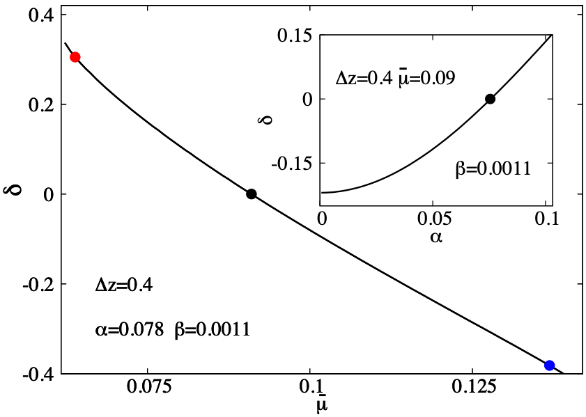
Figure 2: The conical excess/deficit $\delta$ as defined by the relation (3.10) is shown as a function of the input parameter $\bar{\mu}$ (related to the horizon size) for 2BHs with real scalar hair ($m=0$). The coordinate distance (parameter) between the horizons $\Delta z$ is fixed, as well the theory parameters $\alpha,\beta$. The three dots correspond to the solutions displayed in Fig. 3. The inset shows a similar plot, with $\delta$ as a function of the theory parameter $\alpha$ which measures the strength of gravity. The balanced configurations are highlighted with black dots.

These symmetries are used in practice to simplify the numerical study of the solutions. First, the symmetry (4.3) is employed to work in units of length set by the scalar field mass,

$$\tilde{\mu}=1\ ,\qquad i.e.\quad c=\frac{1}{\mu}\ .$$ (4.6)

The second symmetry (4.5) is used to set to unity the coefficient of the quartic term in the scalar field potential,

$$\bar{\lambda}=1\ ,\qquad i.e.\quad c=\frac{1}{\sqrt{\lambda}}\ .$$ (4.7)

It follows that two mass scales naturally emerge, one set by gravity, $M_{\rm Pl}\equiv 1/\sqrt{G}$, and the other one set by the scalar field parameters, $M_{0}\equiv\mu{/\sqrt{\lambda}}$. The ratio of these fundamental mass scales defines the dimensionless coupling constant

$$\alpha\equiv\frac{M_{0}}{M_{\rm Pl}}\ ,$$ (4.8)

which is relevant in the physics of the solutions.

Apart from $\alpha$, the second dimensionless input parameter is the (scaled) constant for the sextic term in the scalar potential, with

$$\beta\equiv\frac{\nu\mu^{2}}{\lambda^{2}}\ .$$ (4.9)

Then, the scaled scalar potential reads $U(\phi)=\phi^{2}-\phi^{4}+\beta\phi^{6},$ while the Einstein equations become $R_{\alpha\beta}-\frac{1}{2}g_{\alpha\beta}=2\alpha^{2}T_{\alpha\beta}.$

To summarize, after using the scaling symmetries, the problem still possesses four input parameters:

$$\{\alpha,~{}~{}\beta\}~{}~{}{\rm and}~{}~{}\{\Delta z,~{}~{}\bar{\mu}\}\ ,$$ (4.10)

two of them determined by the scalar field potential and the other two by the BW background ”seed” solution. In the solutions with scalar hair, $\Delta z$ and $\bar{\mu}$ are still correlated with, but not strictly corresponding to, the distance between the horizons and the horizons mass, respectively.

All quantities shown in this work are given in natural units set by $G$ and $\mu$, which, in order to simplify the plots, we take to unity in what follows.

                                               

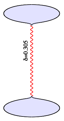
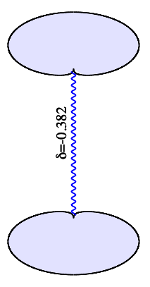
Figure 3: The effective horizon shape is shown for three different 2BH solutions with real scalar hair highlighted with (red, black, and blue) dots in Fig. 2. The coordinate distance between the horizons is $\Delta z=0.4$, while $\bar{\mu}=0.064,$ $0.091$, and $0.137$, respectively (from left to the right). There is string for $\delta>0$ (leftmost panel) and a strut for $\delta<0$ (rightmost panel), connecting the two horizons. The middle configuration is balanced.

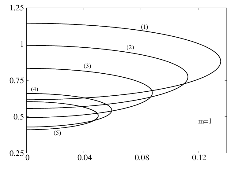
Figure 4: Profiles of the horizon embedding in $\mathbb{E}^{3}$ for the first (”upper”) BH are shown for a set of $m=1$ balanced solutions marked in Fig. 6. The distance between the BHs decreases from (1) to (5).

4.2 The balanced 2BHs system with scalar hair

The decoupling limit $\alpha\to 0$, where $\alpha$ defines the coupling of the scalar field to gravity as given by (4.8), corresponds to solutions of the scalar field equation (2.7) on a fixed BW geometry, $i.e.$ (3.1) with (3.2) and (2.17)-(2.19) (thus, $F_{i}=0$). Some basic properties of the self-gravitating solutions are already present in this case. First, they possess an odd-parity scalar field, describing a configuration with two constituents located at $z=\pm z_{0}$, with $z_{0}$ fixed by the maximum of the energy density, as resulting from numerics. For all solutions in this work (including the ones with scalar back-reaction), we have found that $z_{0}>\Delta z+\bar{\mu}$. An interesting feature of the decoupling limit analysis is that the scalar field never trivializes; we could not find any indication for the existence of linear scalar clouds on a BW background. Also, although more work is necessary, these non-linear cloud solutions appear to exist for arbitrary values of the BW parameters $\Delta z,\bar{\mu}$.

The backreaction is included by starting with the solutions in the decoupling limit, $i.e.$ with given scalar field parameter $\beta$ and BW background parameters $(\Delta z,\bar{\mu})$, and slowly increasing the coupling $\alpha$. Most of the qualitative features of the BW solution are still preserved by their generalizations with scalar hair obtained in this way. The generic solutions possess a conical singularity which prevents their collapse, and no other pathologies. Moreover, by using the formalism in [3], one can show that the hairy solutions with conical singularities still admit a consistent thermodynamical description. In particular, when working with the appropriate set of thermodynamical variables, the Bekenstein-Hawking law still holds, with the entropy $S=A_{H}/4$.

The key aspect we wish to emphasise here is the evolution of the conical singularity strength $\delta$ with increasing $\alpha$. While $\delta<0$ in the decoupling limit, one finds that $|\delta|$ decreases as $\alpha$ increases, with the existence of a critical value $\alpha_{c}$ where $\delta=0$, $i.e.$ a balanced configuration. Moreover, $\delta$ becomes positive for $\alpha>\alpha_{c}$. This behaviour is shown for illustrative values of $(\Delta z,\bar{\mu})$ in the inset of Fig. 2.

A more physical scanning of the solutions, on the other hand, fixes the theory, $i.e.$ fixes ($\alpha$, $\beta$), which are constants of the model. Then a sequences of balanced solutions in a given theory can be found by fixing the parameter $\Delta z$ (related to the coordinate distance between the two BHs) and varying the input parameter $\bar{\mu}$ (related to the BH size). As seen in the main panel of Fig. 2 the system becomes balanced for a critical value of the parameter $\bar{\mu}$, only. For larger (smaller) $\bar{\mu}$ the BHs are too heavy (light) and there is a conical excess/strut (deficit/string) in between them. This is illustrated in Fig. 3, where we display the horizon shape, as given by the effective-radius function ${\rm R}$, relation (3.7), for the three solutions highlighted with (red, black and blue) dots in Fig. 2. By repeating this procedure a (continuous) set of balanced solutions is found by varying the input parameter $\Delta z$ and ’shooting’ for the critical values of $\bar{\mu}$ which give $\delta=0$. To summarize, by varying the value of $\Delta z$ and by adjusting the value of $\bar{\mu}$ via a ’shooting’ algorithm, the full spectrum of balanced 2BHs with given $(\alpha,\beta)$ can be recovered numerically, in principle.

The balanced solutions have no singularities on and outside the horizon. This can be seen by computing the Ricci or the Kretschmann scalars, which are found to be finite everywhere. The scalar field is distributed around the two horizons. But we have found that the energy density, as given by the component $T_{t}^{t}$ of the energy-momentum tensor always becomes negative in a region around the horizons. This also holds for the Komar mass-energy density $T_{\alpha}^{\alpha}-2T_{t}^{t}$ - see the left panel in Fig. 5 –, although its integral (3.14) is always positive. The scalar field profile is a also smooth function – Fig. 5 (right panel).

     

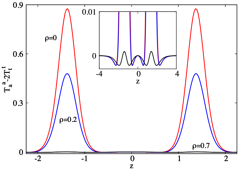
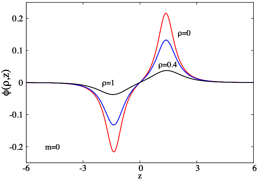
Figure 5: The Komar mass-energy density (left panel) and the scalar field amplitude (right panel) are shown for a typical balanced $m=0$ 2BHs system with scalar hair. The theory constants are $\alpha=0.0775$, $\beta=0.0011$ and geometric input parameters are $\Delta z=1.24$, $\bar{\mu}=0.071$.

     

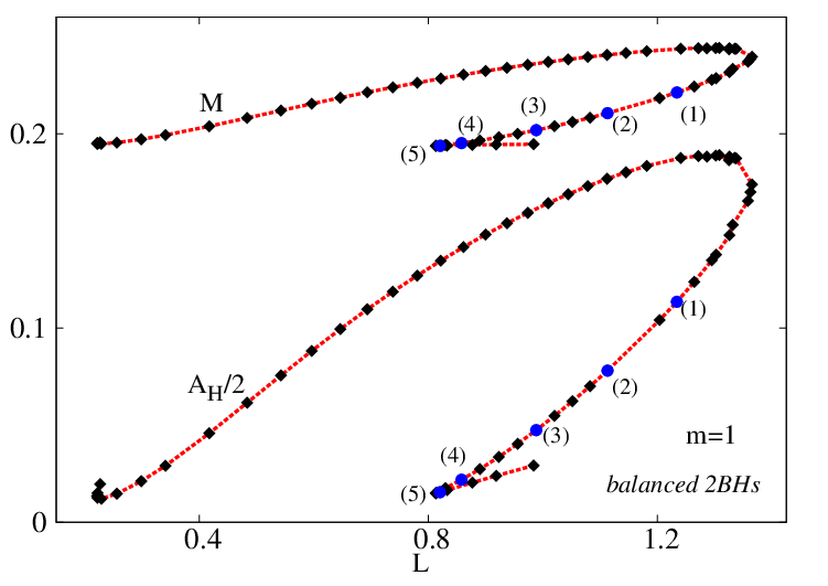
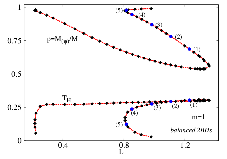
Figure 6: The ADM mass $M$, the horizon area $A_{H}$ (left panel), the hairiness parameter $p$ and the Hawking temperature (right panel) of the balanced 2BHs system with $m=1$, as functions of the proper distance $L$ between the horizons.

A full scanning of the parameter space of balanced solutions is beyond the purposes of this work. We shall focus on balanced solutions with a fixed set of the theory parameters $(\alpha=0.0775,$ $\beta=0.0011)$ and $m=1$, which we have studied more systematically. It is reasonable to expect, albeit unproven, that one such case captures the basic features of the full space of solutions, at least for a nonzero $m$. We emphasise, moreover, that we have established the existence of balanced solutions for other choices of $(\alpha,\beta)$.

The numerical results indicate that, once the model is fixed, there exists a continuous set of balanced solutions, which can be labelled by $L$, the proper distance between the horizons. The most relevant quantities resulting from numerics are shown in Fig. 6 as a function of $L$ (we recall that all quantities there are given in units set by $\mu$ and $G$). One observes that the solutions exist for a finite range of the proper distance, only (with $L_{\rm min}>0$). Thus, although one may expect to find balanced solutions with an arbitrary small or large $L$, this is not confirmed by numerics. Moreover, one, two or even three different solution may exist for a given proper distance between the horizons, with a complicated branch structure in terms of $L$.

One observes that all relevant quantities vary significantly as $L$ varies. Moreover, as expected from the study in the decoupling limit, $p$ never vanishes, and it attains a minimal value at $L_{\rm max}$. Thus, for any distance $L$, a fraction of the spacetime energy must be stored in the scalar hair.

Concerning the behaviour of the solutions at the end of the $L$-interval, the numerical results suggest the existence of two limiting configurations with nonzero values for both $M$ and $A_{H}$, while the Hawking temperature vanishes, see right panel in Fig. 6. Although we could not obtain accurate enough solutions closer to these critical configurations, they are likely singular, with a divergent Ricci scalar outside the horizon.

On general grounds, we expect all 2BH balanced solutions to be unstable against small perturbation, since their existence requires a fine-tunning between the BHs parameters. This is supported by the observation that, for any value of the mass, the configuration maximizing the entropy corresponds to a (single) Schwarzschild vacuum BH, and not to a hairy 2BHs solution.

5 Further remarks

The asymptotically flat static 2BHs system in “vacuum” GR necessarily possesses a conical singularity. A main purpose of this work is to report the existence of static, balanced 2BHs configurations in Einstein-scalar models, without any electromagnetic fields and keeping asymptotic flatness. The solutions are supported by the existence of negative energy densities, as allowed by a choice of a scalar potential which is not strictly positive. Our study indicates the existence of a one-parameter family of balanced solutions, which can be parametrized by the physical distance between the horizons. Our approach is non-perturbative, by solving directly the Einstein-scalar field equations in a Weyl-type coordinate system, subject to proper boundary conditions.

In fact, the considered Einstein-scalar theory can be taken as a simple toy-model for other cases which may be physically more interesting, for instance avoiding negative scalar energies. Similar solutions are likely to exist in a variety of other models, with similar mechanisms at work. For example, effective negative energy densities naturally occur in a theories with a Gauss-Bonnet term non-minimally coupled with a scalar field, see $e.g.$ [43, 44]. Therefore it is natural to conjecture the existence of static balanced 2BHs solutions also in such models, although their investigation whould be a more intricate task, by virtue of the complexity of the equations of motion.

Another possible balancing mechanism is to include the effects of rotation. This is suggested by the situation with the black rings in five spacetime dimensions [22]. In that case, the static black ring is unbalanced, being supported against collapse by conical singularities [27]. Adding rotation balances the ring for a critical value of the event horizon velocity [22]. One may expect that co-rotation of two BHs may help to alleviate the need for negative energies, within four dimensional (non-vacuum) 2BH solutions. Indeed, one may consider the existence of spinning balanced binary BHs in a model with a complex massive scalar field without self-interations or negative scalar energies, where the existence of hair is allowed via the synchronization mechanism [48, 49].

Appendix A Field equations in the parameterization (3.1)

For model (2.1), with the ansatz (3.1) and (2.5), an appropriate combination of the Einstein equations, $E_{t}^{t}=0$, $E_{\rho}^{\rho}+E_{z}^{z}=0$ and $E_{\varphi}^{\varphi}=0$, yield the following set of equations for the functions $f_{0},~{}f_{1}$ and $f_{2}$:

$$\nabla^{2}f_{0}-\frac{1}{2f_{0}}(\nabla f_{0})^{2}+\frac{1}{2f_{2}}(\nabla f_{0})\cdot(\nabla f_{2})+4Gf_{0}f_{1}U(\phi)=0\ ,$$

$$\nabla^{2}f_{1}-\frac{1}{f_{1}}(\nabla f_{1})^{2}-\frac{f_{1}}{2f_{0}f_{2}}(\nabla f_{0})\cdot(\nabla f_{2})+4Gf_{1}\left[(\nabla\phi)^{2}-\frac{m^{2}f_{1}\phi^{2}}{f_{2}}\right]=0\ ,$$

$$\nabla^{2}f_{2}-\frac{1}{2f_{2}}(\nabla f_{2})^{2}+\frac{1}{2f_{0}}(\nabla f_{0})\cdot(\nabla f_{2})+4Gf_{1}(f_{2}U(\phi)+2m^{2}\phi^{2})=0\ .$$ (A.1)

The equation for the scalar field amplitude $\phi$ is

$$\nabla^{2}\phi+\frac{1}{2f_{0}}(\nabla f_{0})\cdot(\nabla\phi)+\frac{1}{2f_{2}}(\nabla f_{2})\cdot(\nabla\phi)-\frac{m^{2}f_{1}}{f_{2}}\phi-\frac{f_{1}}{2}\frac{dU(\phi)}{d\phi}=0\ .$$ (A.2)

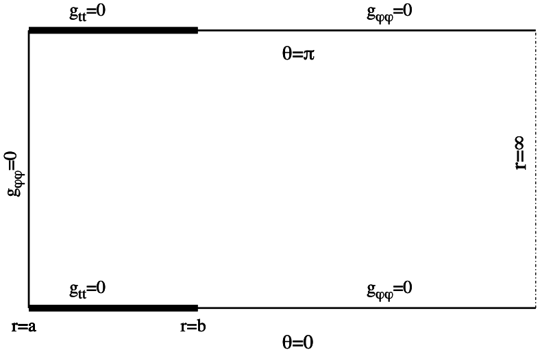
Figure 7: The 2BHs rod structure in Fig. 1 is displayed for $(r,\theta)$-coordinates, as defined by Eq. (B.1).

We have defined, acting on arbitrary functions $\mathcal{F}(\rho,z)$ and $\mathcal{G}(\rho,z)$,

$$(\nabla\mathcal{F})\cdot(\nabla\mathcal{G})\equiv\partial_{\rho}\mathcal{F}\partial_{\rho}\mathcal{G}+\partial_{z}\mathcal{F}\partial_{z}\mathcal{G}\ ,\qquad\nabla^{2}\mathcal{F}\equiv\partial_{\rho}^{2}\mathcal{F}+\partial_{z}^{2}\mathcal{F}\ .$$ (A.3)

Appendix B A new coordinate system and details on the numerics

Even though the 2BHs solutions reported in this paper can be constructed by employing the Weyl-type coordinates $(\rho,z)$, the metric ansatz (3.1) has a number of disadvantages. For example, the coordinate range is unbounded for both $\rho$ and $z$, which makes it difficult to extract with enough accuracy the value of the mass parameter $M$ from the asymptotic form of the metric function $f_{0}$.

Thus, in practice, to solve numerically the Einstein-scalar field equations, we have found it more convenient to introduce the new coordinates $(r,\theta)$ related to $(\rho,z)$ in (3.1) by

$$\rho=\frac{r^{2}-a^{2}}{r}\sin\theta\ ,\qquad z=\frac{r^{2}+a^{2}}{r}\cos\theta\ ,\qquad{\rm with}\qquad\bar{\mu}=\frac{(a-b)^{2}}{b}\ ,\qquad\Delta z=4a\ ,$$ (B.1)

with ranges $a\leqslant r<\infty$ and $0\leqslant\theta\leqslant\pi$, and reparametrize the metric (3.1) as

$$ds^{2}=-\hat{f}_{0}(r,\theta)dt^{2}+{\hat{f}_{1}(r,\theta)}(dr^{2}+r^{2}d\theta^{2})+\hat{f}_{2}(r,\theta)d\varphi^{2}\ .$$ (B.2)

The rod structure in (3.1) is still preserved for the new coordinate system, although it becomes less transparent – see Fig. 7. The two BHs horizons are now located at: (i) $\theta=0$, for $a\leqslant r\leqslant b$; and (ii) at $\theta=\pi$, $a\leqslant r\leqslant b$. The rod separating the BHs is located at $r=a$ and $0\leqslant\theta\leqslant\pi$.

Analogous to the case of Weyl-type coordinates, we define

$$\hat{f}_{i}=\hat{f}_{i}^{0}e^{2\hat{F}_{i}}\ ,$$ (B.4)

with the background functions $\hat{f}_{i}^{0}$ corresponding to the vacuum BW solution expressed in the $(r,\theta)$-coordinates. Their explicit expression reads:

$$\hat{f}_{0}^{0}(r,\theta)=\frac{a^{2}b-(a-b)^{2}r+br^{2}-2abr\cos\theta+\sqrt{(b^{2}+r^{2}-2br\cos\theta)(a^{4}+b^{2}r^{2}-2a^{2}br\cos\theta)}}{-2abr+a^{2}(b+r)+br(b+r)-2abr\cos\theta+\sqrt{(b^{2}+r^{2}-2br\cos\theta)(a^{4}+b^{2}r^{2}-2a^{2}br\cos\theta)}}$$

$${~{}~{}}\times\frac{a^{2}b-(a-b)^{2}r+br^{2}+2abr\cos\theta+\sqrt{(b^{2}+r^{2}+2br\cos\theta)(a^{4}+b^{2}r^{2}+2a^{2}br\cos\theta)}}{-2abr+a^{2}(b+r)+br(b+r)+2abr\cos\theta+\sqrt{(b^{2}+r^{2}+2br\cos\theta)(a^{4}+b^{2}r^{2}+2a^{2}br\cos\theta)}}\ ,$$ (B.5)

$$\hat{f}_{1}^{0}(r,\theta)=\frac{S(r,\theta)\Omega(r,\theta)}{\hat{f}_{0}(r,\theta)}\ ,\qquad\hat{f}_{2}^{0}(r,\theta)=\frac{(r^{2}-a^{2})^{2}\sin^{2}\theta}{r^{2}}\frac{1}{\hat{f}_{0}(r,\theta)}\ ,$$ (B.6)

with

$$S(r,\theta)=\frac{(a^{2}-r^{2})^{2}}{2\sqrt{(b^{4}+r^{4}-2b^{2}r^{2}\cos 2\theta)(a^{8}+b^{4}r^{4}-2a^{4}b^{2}r^{2}\cos 2\theta)}}$$ (B.7)

$$\times\frac{a^{4}b+2a(a^{2}+b^{2})r^{2}+br^{4}-(a+b)^{2}r(a^{2}+r^{2})\cos\theta+2a^{2}br^{2}\cos 2\theta+(a^{2}+r^{2}-2ar\cos\theta)\sqrt{(b^{2}+r^{2}-2br\cos\theta)(a^{4}+b^{2}r^{2}-2a^{2}br\cos\theta)}}{a^{4}+r^{4}-2a^{2}r^{2}\cos 2\theta}$$

$$\times\frac{a^{4}b+2a(a^{2}+b^{2})r^{2}+br^{4}+(a+b)^{2}r(a^{2}+r^{2})\cos\theta+2a^{2}br^{2}\cos 2\theta+(a^{2}+r^{2}+2ar\cos\theta)\sqrt{(b^{2}+r^{2}+2br\cos\theta)(a^{4}+b^{2}r^{2}+2a^{2}br\cos\theta)}}{a^{4}b-2a(a^{2}+b^{2})r^{2}+br^{4}-(a-b)^{2}r(a^{2}+r^{2})\cos\theta+2a^{2}br^{2}\cos 2\theta+(a^{2}+r^{2}+2ar\cos\theta)\sqrt{(b^{2}+r^{2}-2br\cos\theta)(a^{4}+b^{2}r^{2}-2a^{2}br\cos\theta)}}$$

$$\times\frac{a^{4}b^{2}-(a^{2}+b^{2})^{2}+b^{2}r^{4}+2a^{2}b^{2}r^{2}\cos 2\theta+\sqrt{(b^{4}+r^{4}-2b^{2}r^{2}\cos 2\theta)(a^{8}+b^{4}r^{4}-2a^{4}b^{2}r^{2}\cos 2\theta)}}{a^{4}b-2a(a^{2}+b^{2})r^{2}+br^{4}+(a-b)^{2}r(a^{2}+r^{2})\cos\theta+2a^{2}br^{2}\cos 2\theta+(a^{2}+r^{2}-2ar\cos\theta)\sqrt{(b^{2}+r^{2}+2br\cos\theta)(a^{4}+b^{2}r^{2}+2a^{2}br\cos\theta)}}$$

and

$$\Omega(r,\theta)=1+\frac{a^{4}}{r^{4}}-\frac{2a^{2}\cos 2\theta}{r^{2}}\ .$$ (B.8)

With this parameterization, we solve numerically the resulting set of four coupled non-linear elliptic PDEs for the functions $(\hat{F}_{i},\phi)$, subject to the set of boundary conditions we now describe. At $r=a$ one imposes ($i=0,1,2$)

$$\partial_{r}\hat{F}_{i}|_{r=a}=0,~{}\partial_{r}\phi|_{r=a}=0~{}~{}{\rm for}~{}~{}m=0,~{}~{}{\rm and}~{}~{}~{}\phi|_{r=a}=0~{}~{}{\rm for}~{}~{}m\neq 0\ .$$ (B.9)

The constraint equation ${E}_{r}^{\theta}=0$ implies that $\hat{F}_{2}-\hat{F}_{1}|_{r=a}=$const. ($i.e.$ a constant value of the conical deficit/excess $\delta$). At $\theta=0$ the boundary conditions are

$$\partial_{\theta}\hat{F}_{i}|_{\theta=0}=\partial_{\theta}\phi|_{\theta=0}=0\ .$$ (B.10)

where again, the constraint equation ${E}_{r}^{\theta}=0$ requires $\hat{F}_{0}-\hat{F}_{1}=$const. for $a\leqslant r\leqslant b$ ($i.e.$ a constant value of the Hawking temperature). For $r>b$ one finds another supplementary condition, $\hat{F}_{2}=\hat{F}_{1}$, thus the absence of a conical singularity on the outer $z-$axis, while for $m\neq 0$ one imposes $\phi|_{\theta=0}=0$ instead of a Newmann boundary condition. Similar boundary conditions are found for $\theta=\pi.$ At infinity, one imposes the conditions

$$\hat{F}_{i}|_{r=\infty}=\phi|_{r=\infty}=0\ ,$$ (B.11)

Moreover, the problem still possesses a $Z_{2}$-symmetry, which allows to solve the equations for $0\leqslant\theta\leqslant\pi/2$, only. The following boundary conditions are imposed at $\theta=\pi/2$

$$\partial_{\theta}\hat{F}_{i}|_{\theta=\pi/2}=\phi|_{\theta=\pi/2}=0\ .$$ (B.12)

All numerical calculations are performed by using a professional finite difference solver, which uses a Newton-Raphson method. A detailed presentation of the this code is presented in [47]. In our approach, one introduces the new radial variable $x=(r-a)/(c+r)$ (with $c$ a properly chosen constant) which maps the semi-infinite region $[a,\infty)$ to the compact region $[0,1]$. The equations for $\hat{F}_{i}$ are discretized on a non-equidistant grid in $x$ and $\theta$. Typical grids used have sizes around $200\times 50$ points, covering the integration region $[0,1]\times[0,\pi/2]$. The numerical error for the solutions reported in this work is estimated to be typically $<10^{-3}$. However, the errors increase when studying solutions with small $a$ and for $b$ much larger than $a$ ($i.e.$ a large separation of the BHs).

Appendix C Numerical construction of the 2RNBHs solution

     

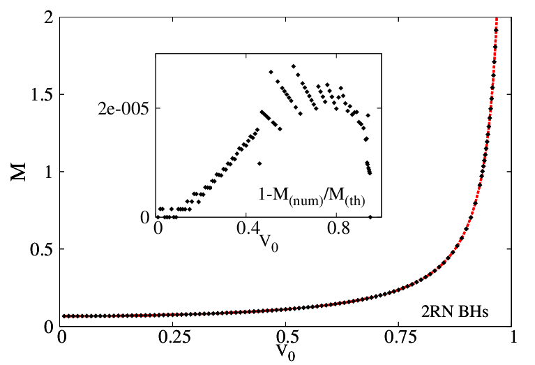
Figure 8: The mass $M$ and the Hawking temperature $T_{H}$ of the 2RNBHs system are shown as a function of the electrostatic potential $V_{0}$ for both theory (red line) and numerical results (dots). The insets show the relative difference. The geometric input parameters are $a=0.1$, $b=0.221$.

The simplest application of the proposed formalism consists in recovering the double Reissner-Nordström solution by solving numerically the Einstein-Maxwell equations

$$R_{\alpha\beta}-\frac{1}{2}g_{\alpha\beta}R=2G\left(F_{\alpha\gamma}F_{\beta}^{\gamma}-\frac{1}{4}g_{\alpha\beta}F^{2}\right)\ ,~{}~{}~{}\nabla_{\alpha}F^{\alpha\beta}=0\ ,$$ (C.1)

with $F=dA$ the Maxwell field strngth tensor.

Restricting again to a $\mathbb{Z}_{2}$-symmetric solution, we consider the metric ansatz (B.2), (B.4) and a purely electric Maxwell field,

$$A=V(r,\theta)dt~{},$$ (C.2)

and solve numerically the equations for $\hat{F}_{i}$, $V$ by using the approach described above. The boundary conditions satisfied by the electrostatic potential $V$ are

$$\partial_{r}V|_{r=a}=0,~{}~{}V|_{r=\infty}=V_{0},~{}~{}\partial_{\theta}V|_{\theta=\pi/2}=0~{},$$ (C.3)

together with

$$V|_{\theta=0}=0~{}~{}{\rm for}~{}~{}a\leqslant r\leqslant b~{}~{}{\rm and}~{}~{}\partial_{\theta}V|_{\theta=0}=0~{}~{}{\rm for}~{}~{}r>b\ .$$ (C.4)

The numerical approach is similar to that employed for 2BHs with scalar hair, the input parameters being the rod coordinates $\{a,b\}$ together with $V_{0}$. However, the corresponding exact solution is known in this case, and can be written in the form (B.2), (B.4) with

$$e^{2\hat{F}_{0}}=\frac{1}{P^{2}},~{}~{}e^{2\hat{F}_{1}}=e^{2\hat{F}_{1}}=P^{2},~{}~{}V=\frac{\tanh\gamma}{P}\hat{f}_{0}^{0},~{}~{}{\rm with}~{}~{}P=\cosh^{2}\gamma-\sinh^{2}\gamma\hat{f}_{0}^{0}\ ,$$ (C.5)

where $\gamma$ is an (arbitrary) real parameter corresponding to the electrostatic potential of the configurations, $\tanh\gamma=V_{0}$. Then a straightforward computation leads to the following expression of several quantities of interest

$$M=\frac{(a-b)^{2}}{b}\frac{1+V_{0}^{2}}{1-V_{0}^{2}}\ ,\qquad Q_{e}=\frac{2(a-b)^{2}}{b}\frac{V_{0}}{1-V_{0}^{2}}\ ,$$ (C.6)

$$A_{H}=\frac{8\pi(a-b)^{4}(a^{2}+b^{2})}{b^{2}(a+b)^{2}}\frac{1}{(1-V_{0}^{2})^{2}}\ ,\qquad T_{H}=\frac{b(a+b)^{2}}{8\pi(a-b)^{2}(a^{2}+b^{2})}(1-V_{0}^{2})^{2}\ ,~{}~{}$$

with $Q_{e}$ the total electric charge.

In Fig. 8 we show a comparison between the theory and numerical results for the mass and Hawking temperature as a function of $V_{0}$ for some fixed $(a,b)$. The insets there give an overall estimate for the numerical accuracy of the solutions, which is consistent with other diagnostics provided by the solver (similar results hold for $Q_{e}$ and $A_{H}$; also a similar picture is found when varying $a$ or $b$ at fixed $V_{0}$). This supports that the proposed numerical scheme can be used in the construction of multi-BH solutions in the presence of matter fields.

References

- [1] R. Bach and H. Weyl, Math. Z 13 (1922) 134.
- [2] A. Einstein and N. Rosen, Phys. Rev. 49 (1936) 404.
-
[3]
C. Herdeiro, B. Kleihaus, J. Kunz and E. Radu,
Phys. Rev. D 81 (2010), 064013
[arXiv:0912.3386 [gr-qc]];
C. Herdeiro, E. Radu and C. Rebelo, Phys. Rev. D 81 (2010), 104031 [arXiv:1004.3959 [gr-qc]]. - [4] M. S. Costa and M. J. Perry, Nucl. Phys. B 591 (2000) 469 [arXiv:hep-th/0008106].
- [5] W. Israel and K. A. Khan, Nuovo Cim. 33 (1964) 331.
- [6] R. C. Myers, Phys. Rev. D 35 (1987), 455
- [7] M. Astorino and A. Vigano, Phys. Lett. B 820 (2021), 136506 [arXiv:2104.07686 [gr-qc]].
- [8] A. Viganò, “Black holes and solution generating techniques,” [arXiv:2211.00436 [gr-qc]].
- [9] D. Kramer and G. Neugebauer, Phys. Lett. A 75 (1980) 259-261.
- [10] R. M. Wald, Phys. Rev. D 6 (1972), 406-413
- [11] J. ö. Hennig, Class. Quant. Grav. 36 (2019) no.23, 235001 [arXiv:1906.04847 [gr-qc]].
- [12] M. S. Costa, C. A. R. Herdeiro and C. Rebelo, Phys. Rev. D 79 (2009), 123508 [arXiv:0903.0264 [gr-qc]].
- [13] S. D. Majumdar, Phys. Rev. 72 (1947), 390-398
- [14] A. Papapetrou, Proc. Roy. Irish Acad. A 52 (1948), 11-23
- [15] J. B. Hartle and S. W. Hawking, Commun. Math. Phys. 26 (1972), 87-101
- [16] G. W. Gibbons and K. i. Maeda, Nucl. Phys. B 298 (1988), 741-775
- [17] N. J. Cornish and G. W. Gibbons, Class. Quant. Grav. 14 (1997), 1865-1881 [arXiv:gr-qc/9612060 [gr-qc]].
- [18] Y. Chen and E. Teo, JHEP 09 (2012), 085 [arXiv:1208.0415 [hep-th]].
-
[19]
R. Emparan and E. Teo,
Nucl. Phys. B 610 (2001) 190
[arXiv:hep-th/0104206];
R. Emparan, Phys. Rev. D 61 (2000) 104009 [arXiv:hep-th/9906160]. - [20] D. Kastor and J. H. Traschen, Phys. Rev. D 47 (1993), 5370-5375 [arXiv:hep-th/9212035 [hep-th]].
- [21] H. Elvang and P. Figueras, JHEP 05 (2007), 050 [arXiv:hep-th/0701035 [hep-th]].
- [22] R. Emparan and H. S. Reall, Phys. Rev. Lett. 88 (2002), 101101 [arXiv:hep-th/0110260 [hep-th]].
- [23] M. J. Duff, R. R. Khuri and J. X. Lu, Phys. Rept. 259 (1995), 213-326 [arXiv:hep-th/9412184 [hep-th]].
- [24] G. W. Gibbons and C. M. Hull, Phys. Lett. B 109 (1982), 190-194
- [25] K. P. Tod, Phys. Lett. B 121 (1983), 241-244
- [26] H. Weyl, Ann. Physik 54 (1917) 117; Ann. Physik 54 (1917) 185.
- [27] R. Emparan and H. S. Reall, Phys. Rev. D 65 (2002), 084025 [arXiv:hep-th/0110258 [hep-th]].
- [28] T. Harmark, Phys. Rev. D 70 (2004), 124002 [arXiv:hep-th/0408141 [hep-th]].
- [29] V. A. Belinsky and V. E. Zakharov, Sov. Phys. JETP 48 (1978), 985-994
- [30] V. A. Belinsky, Sov. Phys. JETP 50 (1979), 623-631
- [31] M. Astorino, Phys. Rev. D 91 (2015), 064066 [arXiv:1412.3539 [gr-qc]].
- [32] J. D. Bekenstein, Phys. Rev. Lett. 28 (1972), 452-455
- [33] C. A. R. Herdeiro and E. Radu, Int. J. Mod. Phys. D 24 (2015) no.09, 1542014 [arXiv:1504.08209 [gr-qc]].
- [34] U. Nucamendi and M. Salgado, Phys. Rev. D 68 (2003), 044026 [arXiv:gr-qc/0301062 [gr-qc]].
- [35] S. S. Gubser, Class. Quant. Grav. 22 (2005), 5121-5144 [arXiv:hep-th/0505189 [hep-th]].
- [36] B. Kleihaus, J. Kunz, E. Radu and B. Subagyo, Phys. Lett. B 725 (2013), 489-494 [arXiv:1306.4616 [gr-qc]].
- [37] A. Bakopoulos and T. Nakas, JHEP 04 (2022), 096 [arXiv:2107.05656 [gr-qc]].
- [38] T. Wiseman, Class. Quant. Grav. 20 (2003) 1137 [arXiv:hep-th/0209051].
- [39] J. M. Bardeen, B. Carter and S. W. Hawking, Commun. Math. Phys. 31 (1973) 161.
- [40] J. F. M. Delgado, C. A. R. Herdeiro and E. Radu, Phys. Rev. D 94 (2016) no.2, 024006 [arXiv:1606.07900 [gr-qc]].
-
[41]
B. Kleihaus, J. Kunz and E. Radu,
Phys. Lett. B 678 (2009), 301-307
[arXiv:0904.2723 [hep-th]];
B. Kleihaus, J. Kunz, E. Radu and M. J. Rodriguez, JHEP 02 (2011), 058 [arXiv:1010.2898 [gr-qc]];
B. Kleihaus, J. Kunz and K. Schnulle, Phys. Lett. B 699 (2011), 192-198 [arXiv:1012.5044 [hep-th]];
B. Kleihaus, J. Kunz and E. Radu, Phys. Lett. B 718 (2013), 1073-1077 [arXiv:1205.5437 [hep-th]]. - [42] S. R. Coleman, Nucl. Phys. B 262 (1985) no.2, 263
- [43] B. Kleihaus, J. Kunz, S. Mojica and E. Radu, Phys. Rev. D 93 (2016) no.4, 044047 [arXiv:1511.05513 [gr-qc]].
- [44] J. F. M. Delgado, C. A. R. Herdeiro and E. Radu, JHEP 04 (2020), 180 [arXiv:2002.05012 [gr-qc]].
- [45] C. A. R. Herdeiro and C. Rebelo, JHEP 10 (2008), 017 [arXiv:0808.3941 [gr-qc]].
- [46] L. Smarr, Phys. Rev. D 7 (1973), 289-295
-
[47]
W. Schönauer and R. Weiß,
J. Comput. Appl. Math. 27, 279 (1989) 279;
M. Schauder, R. Weiß and W. Schönauer, The CADSOL Program Package, Universität Karlsruhe, Interner Bericht Nr. 46/92 (1992). - [48] C. A. R. Herdeiro and E. Radu, Phys. Rev. Lett. 112 (2014), 221101 [arXiv:1403.2757 [gr-qc]].
- [49] C. A. R. Herdeiro and E. Radu, Int. J. Mod. Phys. D 23 (2014) no.12, 1442014 [arXiv:1405.3696 [gr-qc]].