Symmetry constraints and spectral crossing in a Mott insulator
with Green’s function zeros

Abstract

Lattice symmetries are central to the characterization of electronic topology. Recently, it was shown that Green’s function eigenvectors form a representation of the space group. This formulation has allowed the identification of gapless topological states even when quasiparticles are absent. Here we demonstrate the profundity of the framework in the extreme case, when interactions lead to a Mott insulator, through a solvable model with long-range interactions. We find that both Mott poles and zeros are subject to the symmetry constraints, and relate the symmetry-enforced spectral crossings to degeneracies of the original non-interacting eigenstates. Our results lead to new understandings of topological quantum materials and highlight the utility of interacting Green’s functions toward their symmetry-based design.

Introduction:

In band theory of non-interacting topological semimetals, lattice symmetries act as indicators of topology and have been widely exploited in identifying novel topological materials  Armitage et al. (2018); Nagaosa et al. (2020); Bradlyn et al. (2017); Cano et al. (2018); Po et al. (2017); Watanabe et al. (2016); Cano and Bradlyn (2021). The effects of interactions in topological semimetals are typically analyzed perturbatively Armitage et al. (2018); Son (2007); Sun et al. (2009); Vafek and Yang (2010); Herbut et al. (2009); Sur and Nandkishore (2016); Huh et al. (2016); Roy (2017); Sur and Roy (2019). To address the interplay between strong correlations and topology, however, non-perturbative approaches to the interactions are required. Whether and how symmetry constraints operate is a priori unclear.

Recently, a group that includes several of us have shown that the Green’s function eigenvectors form a representation of the space group Hu et al. (2021), in parallel to the Bloch functions of the non-interacting settings Cano and Bradlyn (2021). Symmetry enforced or protected degeneracies then respectively follow when the dimensionality of irreducible representation is greater than one at a given high symmetry point, or when two irreducible representations with distinct symmetry eigenvalues cross along a high symmetry line. This formulation was applied to the case of a multi-channel Kondo lattice, which features dispersive modes with fractionalized electronic excitations. The eigenvectors of the Green’s function were used to define degeneracies by locating spectral crossings Hu et al. (2021). The approach also provided the theoretical basis for the robustness Chen et al. (2022a) of Kondo-driven Weyl semimetals Lai et al. (2018); Dzsaber et al. (2017, 2021).

The extreme form of correlation effects occurs when the interactions drive a metal into a Mott localized state. It is an intriguing question as to what role topological nodes of the non-interacting limit may have in Mott insulators Morimoto and Nagaosa (2016). Along this direction, determining how symmetry constraints operate in a Mott insulator represents an outstanding open question. One of the important features of a Mott insulator is that it can have Green’s function poles and zeros, both of which contribute to the Luttinger count of electronic states Abrikosov et al. (2012). Does symmetry constrain both features?

In this work, we address the symmetry constraints of a Mott insulator using the Green’s function approach Hu et al. (2021). To be specific, we present our analysis on a lattice model in which the non-interacting Hamiltonian has symmetry-enforced Dirac nodes, though we expect our results to be valid more generally. Importantly, the symmetry constrains the Green’s functions at all frequencies and the degeneracies at the high symmetry wavevectors appear in the form of spectral crossings; in particular, we find that this operates on both Green’s function poles and zeros. Our qualitative results are illustrated in Fig. 1: the spectral crossings of the Green’s function poles [(c)] and Green’s function zeros [(d)] appears as the wavector moves [(b)] towards the high symmetry wavevector $P$; this captures the degereracy of the Green’s function eigenvectors at $P$, where the Bloch functions of the non-interacting counterpart are degenerate [(a), top panel]. They give rise to new understandings of topological quantum materials and set the stage for systematic analysis of the topology of Mott insulators.

Interacting square net lattice and solution method: We consider a two-dimensional (2D) square net lattice, as illustrated in Fig. 2. Here, the non-interacting bands contain symmetry enforced Dirac crossings at the $X$ and $M$ points in the Brillouin zone (Fig. 1(a), bottom panel)  Young and Kane (2015). We focus on local in momentum interactions analogous to those appearing in the Hatsugai-Kohmoto (HK) model Hatsugai and Kohmoto (1992); Morimoto and Nagaosa (2016); Phillips et al. (2018); Setty (2020, 2021a); Phillips et al. (2020); Huang et al. (2021); Yang (2021); Zhu et al. (2021); Setty (2021b); Fabrizio (2022). This form of interaction can be solved exactly [see the Supplementary Material (SM), Sec. C], which facilitates the understanding of not only the symmetry-enforced spectral crossing but also the symmetry constraints on dispersive poles and zeros as we do below.

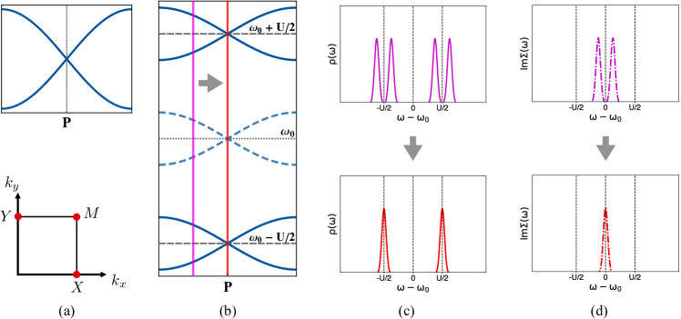
Figure 1: Schematic summary of symmetry constraints and spectral crossings in a Mott insulator with Green’s functions zeros and poles (a) Top: Symmetry enforced Dirac point in the non-interacting dispersion that occurs at a high symmetry point $P$. Bottom: Dirac points (red dots) that occur in the square net lattice at high symmetry points in the Brillouin zone. (b) Symmetry enforced spectral crossings in the Mott insulator state. They involve the upper and lower Hubbard bands (solid curves) and their associated Dirac points are separated by $U$ and a contour of crossings of zeros (dashed curves). Both are enforced by the lattice symmetry. (c) Top: Spectral function (imaginary part of the Green’s function) at a wavevector marked by the magenta line in (b) away from the Dirac point for the poles of the Green’s function. Bottom: Spectral function at the wavevector $P$ marked by the red line in (b) at the Dirac point. (d) Top: Imaginary part of the self energy at a wavevector marked by the magenta line in (b) indicating zeros of the Green’s function. Bottom: Same at the wavevector $P$ marked by the red line indicating degeneracies of zeros enforced by symmetry.

The Hamiltonian of a 2D square net lattice (Fig. 2) in the orbital basis $\Lambda_{\bm{k}}^{\intercal}\equiv(c_{A,\Uparrow},c_{A,\Downarrow},c_{B,\Uparrow},c_{B,\Downarrow})_{\bm{k}}$ takes the form $\tilde{\mathscr{H}}=\tilde{\mathscr{H}}_{0}+\tilde{\mathscr{H}}_{I}$, where

$$\tilde{\mathscr{H}}_{0}=\sum_{\bm{k}}\Lambda_{\bm{k}}^{\dagger}\tilde{h}_{0}(\bm{k})\Lambda_{\bm{k}}$$

$$\tilde{\mathscr{H}}_{I}=\frac{\alpha}{2}\sum_{\bm{k}}\Lambda_{\bm{k}}^{\dagger}\Lambda_{\bm{k}}+\frac{U_{c}}{2}\sum_{\bm{k}}\left(\Lambda_{\bm{k}}^{\dagger}\Lambda_{\bm{k}}\right)^{2}$$

$$\qquad+\frac{U_{s}}{2}\sum_{\bm{k}}\quantity(\Lambda_{\bm{k}}^{\dagger}\tau_{1}\otimes\sigma_{0}\Lambda_{\bm{k}})^{2}$$ (1)

with $\tilde{h}_{0}(\bm{k})=t_{2}(\cos{k_{x}}+\cos{k_{y}})\mathbbm{1}+2t\cos{\frac{k_{x}}{2}}\cos{\frac{k_{y}}{2}}\tau_{1}\otimes\sigma_{0}+t_{SO}\left[\sin{k_{x}}\tau_{3}\otimes\sigma_{2}-\sin{k_{y}}\tau_{3}\otimes\sigma_{1}\right]-\mu\mathbbm{1}$, $\tau_{j}$ ($\sigma_{j}$) being the $j$-th Pauli matrix acting on the sublattice (spin) subspace, and $\mathbbm{1}$ is the $4\times 4$ identity matrix. Here, $c_{a,b}$ are the annihilation operators for electrons in the original sublattice $a=A,B$ and physical spin $b=\Uparrow,\Downarrow$ indices. $t,t_{2}$ are the hopping parameters, $t_{SO}$ is the spin-orbit coupling, $U_{c}$ and $U_{s}$ are intra- and inter-orbital interaction, respectively, and $\alpha$ is a constant shift in the density which we fix to $-(U_{c}+U_{s})$ for convenience. Without loss of generality, henceforth, we set $t_{2}=0$.

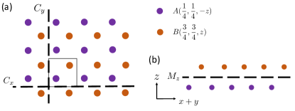
Figure 2: (a) The top view of the 2D square net lattice. The purple and orange dots denote the $A$ and $B$ sublattices in different $z$ planes. $C_{x}$ and $C_{y}$ mark the non-symmorphic rotational symmetries. (b) The side view of the lattice along the $x+y$ direction. $M_{z}$ denotes the non-symmorphic glide mirror symmetry.

It is convenient to work in a basis where the non-interacting Hamiltonian is block diagonal. To this end, we rotate the original basis of $\Lambda_{\bm{k}}^{\intercal}$ into the new basis $\Phi_{\bm{k}}^{\intercal}\equiv(\phi_{+,\Uparrow},\phi_{+,\Downarrow},\phi_{-,\Uparrow},\phi_{-,\Downarrow})_{\bm{k}}\equiv\frac{1}{\sqrt{2}}(c_{A,\Uparrow}+c_{B,\Uparrow},c_{A,\Downarrow}-c_{B,\Downarrow},-c_{A,\Uparrow}+c_{B,\Uparrow},c_{A,\Downarrow}+c_{B,\Downarrow})_{\bm{k}}$. This amounts to block-diagonalizing the Hamiltonian matrix as

$$\tilde{h}_{0}(\bm{k})\to h_{0}(\bm{k})=e^{i\frac{\pi}{4}\tau_{2}\otimes\sigma_{3}}\tilde{h}_{0}(\bm{k})e^{-i\frac{\pi}{4}\tau_{2}\otimes\sigma_{3}},$$ (2)

where $h_{0}(\bm{k})=\vec{n}(\bm{k})\cdot\vec{\Gamma}-\mu\mathbbm{1}$ with $\vec{n}(\bm{k})=\quantity{-t_{SO}\sin{k_{y}},t_{SO}\sin{k_{x}},2t\cos{\frac{k_{x}}{2}}\cos{\frac{k_{y}}{2}}}$ and $\vec{\Gamma}=\tau_{3}\otimes\vec{\sigma}$. It supports doubly degenerate bands which disperse as $\tilde{\xi}_{j}=-\mu+(-1)^{j}|\vec{n}(\bm{k})|$. In the $\Phi_{\bm{k}}$ basis,

$$\tilde{\mathscr{H}}_{I}\to{\mathscr{H}}_{I} = \frac{U_{c}}{2}\sum_{\bm{k}}\left(\Phi_{\bm{k}}^{\dagger}\Phi_{\bm{k}}\right)^{2}+\frac{\alpha}{2}\sum_{\bm{k}}\Phi_{\bm{k}}^{\dagger}\Phi_{\bm{k}}$$

$$+ \frac{U_{s}}{2}\sum_{\bm{k}}\quantity(\Phi_{\bm{k}}^{\dagger}\tau_{3}\otimes\sigma_{3}\Phi_{\bm{k}})^{2}.$$

Here $\Phi_{\bm{k}}^{\dagger}\Phi_{\bm{k}}$ is the total charge and $\Phi_{\bm{k}}^{\dagger}\tau_{3}\otimes\sigma_{3}\Phi_{\bm{k}}$ is a staggered pseudo-sublattice density for a given momentum.

In the band basis, $\Psi_{\bm{k}}=(\psi_{1,\uparrow},\psi_{1,\downarrow},\psi_{2,\uparrow},\psi_{2,\downarrow})_{\bm{k}}^{\intercal}$ with $\{\psi_{j,\uparrow},\psi_{j,\downarrow}\}$ representing the $j$-th pair of degenerate bands, $h_{0}$ is diagonalized to $\quantity[-\mu\mathbbm{1}+|\vec{n}(\bm{k})|\tau_{3}\otimes\sigma_{0}]$. Henceforth, we treat $\sigma=\uparrow,\downarrow$ and $i,j=1,2$ as a pseudo-spin and band indices respectively. In the limit of weak spin-orbit coupling, $(t_{SO}/t)\ll 1$, the total Hamiltonian can be cast into the form $H=H_{0}+H_{I}$ with $H_{0}=\sum_{\bm{k}i\sigma}\xi_{i\sigma}(\bm{k})\psi^{\dagger}_{i\sigma}(\bm{k})\psi_{i\sigma}(\bm{k})$ and

$$H_{I}=U\sum_{\bm{k}i}n_{\bm{k}i\uparrow}n_{\bm{k}i\downarrow}+U^{\prime}\sum_{\begin{subarray}{c}\bm{k}\sigma\sigma^{\prime}\\ i\neq j\end{subarray}}n_{\bm{k}i\sigma}n_{\bm{k}j\sigma^{\prime}}+\order{t_{SO}/t},$$ (4)

where $(U,U^{\prime})=(U_{c}+U_{s},U_{c}-U_{s})$, and correspond to intra-band and inter-band interactions respectively. We utilize the density basis to exactly diagonalize the interacting Hamiltonian with interaction terms up to $\order{(t_{SO}/t)^{0}}$. The additional $\order{(t_{SO}/t)^{n>0}}$ terms only distort the bands keeping the degeneracies intact. A full numerical solution for $t\sim t_{SO}$ appears later in the main text and in the SM (Sec. A). The renormalized band dispersions satisfy $\xi_{i\uparrow}(\bm{k})=\xi_{i\downarrow}(\bm{k})$, and are related to the bare band dispersions, $\tilde{\xi}_{i}(\bm{k})$, as $\xi_{i}(\bm{k})\equiv\tilde{\xi}_{i}(\bm{k})-U/2$. The density operators of $\psi_{\bm{k}i\sigma}$ are denoted as $n_{\bm{k}i\sigma}$.

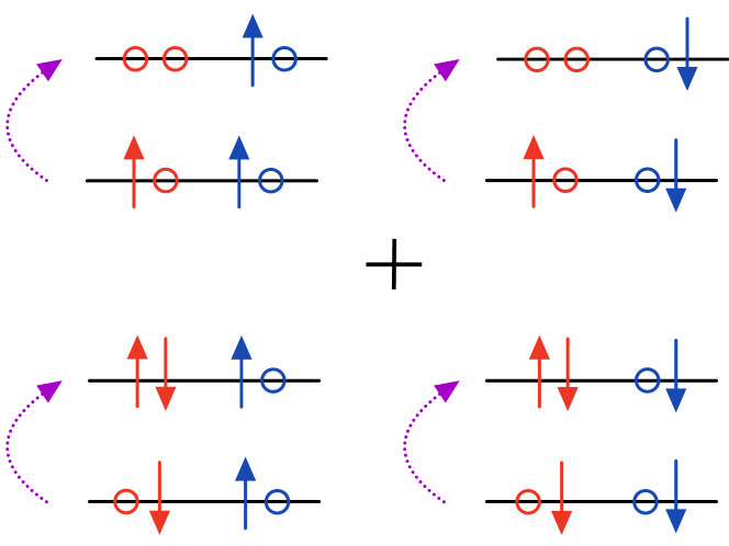
Figure 3: Transitions contributing to the interacting Green’s function in Eq. 7 (or Eq. 25) at a given momentum and zero temperature. The red and blue colors denote the two band degrees of freedom. The circles denote empty states and arrows are pseudo-spin degrees of freedom. The top (bottom) row corresponds to electron removal (addition) states. Their excitation energies are equal and opposite in the presence of time-reversal symmetry. Together, they sum to zero yielding zero surfaces in momentum space.

In the presence of time reversal symmetry, the total Green’s function can be evaluated exactly as outlined in the SM (Sec. B). The calculation captures Fig. 3, which shows the transitions that contribute to the zero of the Green’s function. It simplifies in the zero temperature limit where both $\xi_{1}(\bm{k}),\xi_{2}(\bm{k})$ are filled with $U,U^{\prime}>0$. Further, for each $\bm{k}$, when $U+2U^{\prime}>|\xi_{1}|+2|\xi_{2}|,2|\xi_{1}|+|\xi_{2}|$ and $U>2|\xi_{1}|,2|\xi_{2}|$ but $U^{\prime}<|\xi_{1}|+|\xi_{2}|$, the partition function is $Z_{\bm{k}}=\lim_{\beta\rightarrow\infty}4e^{-\beta(\xi_{1}+\xi_{2}+U^{\prime})}$, and we obtain

$$G(z,\bm{k})=\frac{1}{\tilde{G}^{-1}(z,\bm{k})-(U/2)^{2}\tilde{G}(z,\bm{k})}$$ (5)

in the orbital basis, where $\tilde{G}^{-1}(z,\bm{k})=z\mathbbm{1}-\quantity[\vec{n}(\bm{k})\cdot\vec{\Gamma}-(\mu-U^{\prime})\mathbbm{1}]$. Thus, the net impact of interactions in Eq. (4) is to shift the chemical potential $\mu\to\mu-U^{\prime}$, and generate the self energy,

$$\Sigma(z,\bm{k})=(U/2)^{2}\tilde{G}(z,\bm{k}).$$ (6)

The locations of poles and zeros of $G$ on the complex-$z$ plane are deduced from the roots of the denominator and numerator, respectively, of its determinant,

$$\det{G(z,\bm{k})}=\frac{\quantity[(z+(\mu-U^{\prime}))^{2}-|\vec{n}(\bm{k})|^{2}]^{2}}{\quantity[(z+(\mu-U^{\prime}))^{2}-\quantity(\frac{U}{2}+|\vec{n}(\bm{k})|)^{2}]^{2}\quantity[(z+(\mu-U^{\prime}))^{2}-\quantity(\frac{U}{2}-|\vec{n}(\bm{k})|)^{2}]^{2}}.$$ (7)

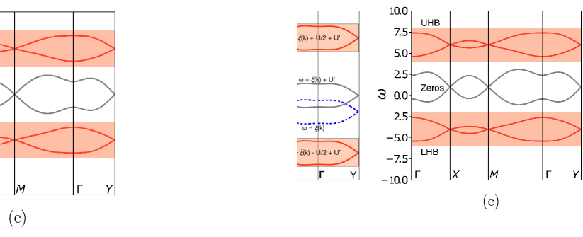
Figure 4: Exact poles and zeros of the total Green’s function of an interacting Dirac semimetal at zero temperature. (a) The upper and lower Hubbard bands (red curves marked UHB and LHB, respectively) and zeros (gray) obtained from analytical diagonalization of the interacting Hamiltonian in the $t_{SO}/t\ll 1$ limit at $U^{\prime}=0$. The blue dotted curve is the original non-interacting band structure which transforms to zeros at sufficiently strong $U$. The green arrow marks the chemical potential. (b) Same as (a) but for $U^{\prime}>0$. Here the contours of zeros and poles are shifted by $U^{\prime}$. (c) The spectrum of the Green’s function obtained by numerical exact diagonalization of the interacting Hamiltonian with $(t,t_{SO},\mu)=(0.7,0.42,5)$ and $(U,U^{\prime})=(10,0.5)$.

Green’s function poles and zeros:

When $U^{\prime}=0$, we have two decoupled copies of Dirac bands with only intraband interaction $U$. When both bands are below the chemical potential, we can treat the two bands separately and use the one band formula (Eq. 28 in SM) for the individual bands. The partition function is simply a product of that for the individual bands and is given by $Z=\prod_{\bm{k}}\prod_{i=i,2}Z_{\bm{k}i}$ with $Z_{\bm{k}i}=1+2e^{-\beta\xi_{i}(\bm{k})}+e^{-\beta\left(2\xi_{i}({\bm{k}})+U\right)}$. Each band is split into a lower and upper Hubbard band with a crossing of zeros at the energies of the original non-interacting bands. A schematic of the various crossings is shown Fig. 4(a).

The spectral function of the interacting Dirac semimetal model at $U^{\prime}\neq 0$ is shown in Fig. 4(b). The spectral functions are analogous to the case of $U^{\prime}=0$ but with the bands shifted by $U^{\prime}$. Additionally, the contour of zeros splits from the original non-interacting bands (dashed blue curves). The features of $G$ obtained in the limit of weak spin-orbit coupling, $(t_{SO}/t)\ll 1$, persists at more generic values of $(t_{SO}/t)$, as demonstrated by numerically diagonalizing the interacting Hamiltonian in Fig. 4(c).

Breaking time-reversal symmetry lifts the twofold degeneracy of the bands in the non-interacting limit. In the interacting model, we introduced an external Zeeman field which splits the pseudo-spins by an energy difference $h$ and studied the robustness of our results. We find that, while broken time reversal symmetry can generically remove zero surfaces, the crossings of poles protected by symmetry are robust. Sec. F of SM contains details of our calculations.

Symmetry constraints and spectral crossings:

The Green’s function eigenvectors form a representation of the space group, as formulated in Ref. Hu et al. (2021) (and briefly summarized in the SM, Sec. D), and are expected to form four-fold degeneracies at the wavevectors $X$, $Y$ and $M$: As in the non-interacting case Young and Kane (2015), the degeneracies at the $X$/$Y$ points are protected by $\{M_{z}|\frac{1}{2}\frac{1}{2}\}$ non-symmorphic mirror symmetry or $\{C_{2x}|\frac{1}{2}0\}$/$\{C_{2y}|0\frac{1}{2}\}$ non-symmorphic screw-axis rotations, while those at the $M$ point are also protected by the $\{C_{2x}|\frac{1}{2}0\}$ and $\{C_{2y}|0\frac{1}{2}\}$ non-symmorphic rotations. Our results for all three cases, with $t_{SO}/t\ll 1$ and $U^{\prime}=0$ [Fig. 4(a)] and $U^{\prime}\neq 0$ [Fig. 4(b)] as well as for the case of unconstrained ratio $t_{SO}/t$ [Fig. 4(c)], demonstrate that the entire spectra obey such degeneracies. This is so even though the system is a Mott insulator with a spectral gap. Moreover, the spectral crossing also applies to the Green’s function zeros. While for the cases (a) and (b), $G(z,\bm{k})$ is diagonal in the same basis that diagonalized the non-interacting Hamiltonian [see the SM (Sec. E)], this special property does not apply to the case (c) nor to the other cases that we have analyzed [see the SM, Fig. 5(d)(e)]. Our results, thus, illustrate our central point, namely the eigenvectors and eigenvalues of the Green’s function can be used to define degeneracies by locating spectral crossings of strongly correlated systems.

Discussion:

Several remarks are in order. First, here we have considered the various cases of the interactions and demonstrated the existence of both poles and zeros of the interacting Green’s function that cross at high-symmetry locations. These crossings are enforced by space group symmetries. For more generic interactions, we expect an extended regime of interactions where the Green’s function zeros persist and the crossings of the poles and zeros continue to be enforced by lattice symmetries. In the SM, Sec. A, we have studied all possible symmetry allowed interaction terms for the square net lattice. We find our conclusions are robust as has been illustrated in Fig. 1. Second, we have used both the Green’s function poles and zeros to illustrate the point that the spectral crossings occur at distinct energies. That the crossings of various bands of poles and zeros can be treated separately, depending on the choice of frequency, highlights a distinct advantage of working with Green’s function eigenvectors. We have also demonstrated the symmetry enforced crossings of zeros and poles in another lattice model (diamond lattice Fu et al. (2007); Fu and Kane (2007)) with HK interaction, which can be found in Sec. G in the SM. Third, the kind of spectral crossings we have discussed sets the stage to analyze the form of topology when strong correlations turn a non-interacting topological semimetals into a Mott insulator. Finally, by demonstrating symmetry constraints and spectral crossing in an extreme interacting setting, our work provides support to the work of Ref Hu et al. (2021). There, spectral crossings through symmetry constraints plays a central role in realizing topological semimetals without Landau quasiparticles.

Implications for experiments and materials:

The Green’s function eigenvector formulation Hu et al. (2021) is expected to yield spectral crossings in other symmetry settings. For example, in the case of Bi₂CuO₄ an eight-fold degeneracy is expected at certain high symmetry wavevectors in its non-interacting bandstructure Bradlyn et al. (2016). The system is in fact strongly interacting Di Sante et al. (2017); Goldoni et al. (1994) and we expect that its paramagnetic Mott insulator state (above its Néel temperature of $50$ K Garcia-Munoz et al. (1990)) will feature eight-fold spectral crossings in the form we have described in some detail here. Probing the spectral function by applying a symmetry-breaking perturbation will allow for experimentally revealing this spectral crossing.

Separately, proximity to an orbital-selective Mott insulating state has recently been advanced as a means of generating Kondo-driven topological semimetals in $d$-electron-based systems that host topological flat bands Chen et al. (2022b); Hu and Si (2022). We can expect that the type of spectral crossings of both the peaks and zeros as discussed here may play an important role in such orbital-selective Mott states.

To conclude, we provide a proof-of-principle demonstration of how lattice symmetries can be used to constrain excitations in an extreme limit of strongly correlated systems. Typically in non-interacting systems, eigenstates of the Hamiltonian and their symmetry operators are used to indicate topology by diagnosing conditions for symmetry protected band crossings. For interacting systems, we recently showed that Green’s function eigenvectors form a representation of the lattice space group and can be used to diagnose and realize topology Hu et al. (2021). Here we study an exactly solvable model of a Mott insulator where eigenvectors and eigenvalues of the Green’s function can be used to locate crossings of poles and zeros in momentum space. Together with the realization of topological semimetals without Landau quasiparticles, our work demonstrates the power that the Green’s function formulation of symmetry constraints displays for realizing non-trivial spectral crossings in fully interacting settings. We can expect the approach to be important for the symmetry-based design of topological quantum materials.

Note added: After the completion of this manuscript, a recent work addressing a different model with a focus on the Green’s function zeros and poles in interacting topological insulators became available (N. Wagner et al., arXiv:2301.05588).

Acknowledgment:

We thank N. Nagaosa for a useful discussion. Work at Rice has primarily been supported by the Air Force Office of Scientific Research under Grant No. FA9550-21-1-0356 (C.S. and S.S.), by the National Science Foundation under Grant No. DMR-2220603 (F.X. and Q.S.), and by the Robert A. Welch Foundation Grant No. C-1411 (L.C.). The majority of the computational calculations have been performed on the Shared University Grid at Rice funded by NSF under Grant EIA-0216467, a partnership between Rice University, Sun Microsystems, and Sigma Solutions, Inc., the Big-Data Private-Cloud Research Cyberinfrastructure MRI-award funded by NSF under Grant No. CNS-1338099, and the Extreme Science and Engineering Discovery Environment (XSEDE) by NSF under Grant No. DMR170109. H.H. acknowledges the support of the European Research Council (ERC) under the European Union’s Horizon 2020 research and innovation program (Grant Agreement No. 101020833). Work in Vienna was supported by the Austrian Science Fund (project I 5868-N - FOR 5249 - QUAST) and the ERC (Advanced Grant CorMeTop, No. 101055088). J.C. acknowledges the support of the National Science Foundation under Grant No. DMR-1942447, support from the Alfred P. Sloan Foundation through a Sloan Research Fellowship and the support of the Flatiron Institute, a division of the Simons Foundation. S.P. and Q.S. acknowledge the hospitality of the Aspen Center for Physics, which is supported by NSF grant No. PHY-1607611.

​​​​​​​​​​​​^⊕ csetty@rice.edu
^† shouvik.sur@rice.edu
^∗ These authors contributed equally

I Supplemental Material: Symmetry constraints and Spectral crossing in a Mott insulator with Green’s function zeros

Chandan Setty Shouvik Sur

Appendix A Square net model

Young and Kane constructed a model of 2D Dirac semimetal on a crinkled checkerboard lattice,

$$\tilde{h}_{0} =t_{2}(\cos{k_{x}}+\cos{k_{y}})\mathbbm{1}+2t\cos{\frac{k_{x}}{2}}\cos{\frac{k_{y}}{2}}\tau_{1}\otimes\sigma_{0}$$

$$\quad+t_{SO}\left[\sin{k_{x}}\tau_{3}\otimes\sigma_{2}-\sin{k_{y}}\tau_{3}\otimes\sigma_{1}\right],$$ (8)

where $\tau_{j}$ ($\sigma_{j}$) is the $j$-th Pauli matrix acting on the sublattice (spin) subspace, and $\mathbbm{1}$ is the $4\times 4$ identity matrix. This Hamiltonian can be block-diagonalized as

$$\tilde{h}_{0}\to h_{0}=e^{i\frac{\pi}{4}\tau_{2}\otimes\sigma_{3}}\tilde{h}_{0}e^{-i\frac{\pi}{4}\tau_{2}\otimes\sigma_{3}},$$ (9)

with

$$h_{0} =t_{2}(\cos{k_{x}}+\cos{k_{y}})\mathbbm{1}+2t\cos{\frac{k_{x}}{2}}\cos{\frac{k_{y}}{2}}\tau_{3}\otimes\sigma_{3}$$

$$\quad+t_{SO}\left[\sin{k_{x}}\tau_{3}\otimes\sigma_{2}-\sin{k_{y}}\tau_{3}\otimes\sigma_{1}\right].$$ (10)

We note that the bases for $\tilde{h}_{0}$ and $h_{0}$ are, respectively,

$$\tilde{\Phi}=\matrixquantity(c_{A,\uparrow}\\ c_{A,\downarrow}\\ c_{B,\uparrow}\\ c_{B,\downarrow}),\quad\Phi=\frac{1}{\sqrt{2}}\matrixquantity(c_{A,\uparrow}+c_{B,\uparrow}\\ c_{A,\downarrow}-c_{B,\downarrow}\\ -c_{A,\uparrow}+c_{B,\uparrow}\\ c_{A,\downarrow}+c_{B,\downarrow})\equiv\matrixquantity(\phi_{+,\Uparrow}\\ \phi_{+,\Downarrow}\\ \phi_{-,\Uparrow}\\ \phi_{-,\Downarrow}),$$ (11)

where $A$ and $B$ denote the two sublattices of the checkerboard lattice. For our purpose, it is convenient to set $t_{2}=0$.

As described in Ref. Young and Kane (2015), a combination of the time reversal, inversion, and non-symmorphic symmetries enforces the dimension of the irreducible representation (irrep) and leads to a fourfold degenerate crossing at high symmetry points $X$, $Y$ and $M$ respectively. The present lattice belongs to the layer group $P4/nmm$, with non-symmorphic symmetry $\{M_{z}|\frac{1}{2}\frac{1}{2}\}$, $\{C_{2x}|\frac{1}{2}0\}$ and $\{C_{2y}|0\frac{1}{2}\}$. It has been proved in Ref. Young and Kane (2015) on the original basis that $\{M_{z}|\frac{1}{2}\frac{1}{2}\}$ and $\{C_{2x}|\frac{1}{2}0\}$ enforce the Dirac points at $X$; $\{M_{z}|\frac{1}{2}\frac{1}{2}\}$ and $\{C_{2y}|0\frac{1}{2}\}$ enforce the Dirac points at $Y$; $\{C_{2x}|\frac{1}{2}0\}$ and $\{C_{2y}|0\frac{1}{2}\}$ enforce the Dirac points at $M$. Here, we take the $M$ point as an example and exam the stability of $k\cdot p$ theory near it in the newly rotated basis. Near the $k=M$ point,

$$h_{0}(M+\bm{q})=t_{SO}(\tau_{z}\sigma_{y}q_{x}-\tau_{z}\sigma_{x}q_{y}).$$ (12)

In the rotated basis, at $M$, the time-reversal symmetry $\Theta=i\sigma_{x}K$, the inversion symmetry $P=-\tau_{z}$. The only allowed mass term is $\tau_{z}$, while it is forbidden by the non-symmorphic symmetries $\{C_{2x}|\frac{1}{2}0\}=-\tau_{y}\sigma_{y}$, $\{C_{2y}|0\frac{1}{2}\}=\tau_{y}\sigma_{x}$. Therefore the four-fold Dirac crossing at $M$ is stable.

A.1 Minimal interacting model

We introduce four-fermion interactions that preserve the following global symmetries of $h_{0}$,

• Chiral-$U(1)$: $[h_{0}(\bm{k}),e^{i\eta_{\bm{k}}\tau_{3}\otimes\sigma_{0}}]=0$ with $\eta_{\bm{k}}$ being an arbitrary $\bm{k}$-dependent angle;

• Fourfold rotation about $\bm{k}=0$: $h_{0}(\bm{k})\to h_{0}(\bm{k}^{\prime})=e^{\frac{i\pi}{4}\tau_{3}\otimes\sigma_{3}}h_{0}(\bm{k})e^{-\frac{i\pi}{4}\tau_{3}\otimes\sigma_{3}}$,

to obtain

$$H_{I}(\bm{k})= \frac{U_{c}}{2}\left(\Phi_{\bm{k}}^{\dagger}\Phi_{\bm{k}}-\frac{1}{2}\right)^{2}+V_{03}\quantity(\Phi_{\bm{k}}^{\dagger}\tau_{0}\otimes\sigma_{3}\Phi_{\bm{k}})^{2}+V_{30}\quantity(\Phi_{\bm{k}}^{\dagger}\tau_{3}\otimes\sigma_{0}\Phi_{\bm{k}})^{2}+\frac{U_{s}}{2}\quantity(\Phi_{\bm{k}}^{\dagger}\tau_{3}\otimes\sigma_{3}\Phi_{\bm{k}})^{2}$$

$$+V_{1}^{\prime}\quantity[\quantity(\Phi_{\bm{k}}^{\dagger}\tau_{1}\otimes\sigma_{1}\Phi_{\bm{k}})^{2}+\quantity(\Phi_{\bm{k}}^{\dagger}\tau_{2}\otimes\sigma_{1}\Phi_{\bm{k}})^{2}]+V_{2}^{\prime}\quantity[\quantity(\Phi_{\bm{k}}^{\dagger}\tau_{1}\otimes\sigma_{2}\Phi_{\bm{k}})^{2}+\quantity(\Phi_{\bm{k}}^{\dagger}\tau_{2}\otimes\sigma_{2}\Phi_{\bm{k}})^{2}],$$ (13)

where the unitary transfortion between the two bases $\tilde{\Phi}_{\bm{k}}\to\Phi_{\bm{k}}=e^{i\frac{\pi}{4}\tau_{2}\otimes\sigma_{3}}\tilde{\Phi}_{\bm{k}}$. $h_{0}(\bm{k})$ is diagonalized by the matrix

$$\mathrm{M}_{\bm{k}}=\left(\begin{array}[]{cccc}e^{\frac{i\varphi_{k}}{2}}\cos\left(\frac{\vartheta_{k}}{2}\right)&0&ie^{\frac{i\varphi_{k}}{2}}\sin\left(\frac{\vartheta_{k}}{2}\right)&0\\ ie^{-\frac{1}{2}\left(i\varphi_{k}\right)}\sin\left(\frac{\vartheta_{k}}{2}\right)&0&e^{-\frac{1}{2}\left(i\varphi_{k}\right)}\cos\left(\frac{\vartheta_{k}}{2}\right)&0\\ 0&ie^{\frac{i\varphi_{k}}{2}}\sin\left(\frac{\vartheta_{k}}{2}\right)&0&e^{\frac{i\varphi_{k}}{2}}\cos\left(\frac{\vartheta_{k}}{2}\right)\\ 0&e^{-\frac{1}{2}\left(i\varphi_{k}\right)}\cos\left(\frac{\vartheta_{k}}{2}\right)&0&ie^{-\frac{1}{2}\left(i\varphi_{k}\right)}\sin\left(\frac{\vartheta_{k}}{2}\right)\\ \end{array}\right)$$ (18)

with $\tan\varphi_{\bm{k}}=\sin{k_{x}}/\sin{k_{y}}$ and $\tan{\vartheta_{\bm{k}}}=\quantity(\frac{t_{SO}}{2t}\sqrt{\sin^{2}{k_{x}}+\sin^{2}{k_{y}}})/\quantity(\cos{\frac{k_{x}}{2}}\cos{\frac{k_{y}}{2}})$, such that

$$\mathrm{M}_{\bm{k}}^{\dagger}h_{0}(\bm{k})\mathrm{M}_{\bm{k}}=\sqrt{\quantity(2t\cos{\frac{k_{x}}{2}}\cos{\frac{k_{y}}{2}})^{2}+t_{SO}^{2}\quantity(\sin^{2}{k_{x}}+\sin^{2}{k_{y}})}~{}\tau_{3}\otimes\sigma_{0}.$$ (19)

Therefore, the 1st and 2nd (3rd and 4th) bands are degenerate in energy. In the band basis, the $V_{00}$ and $V_{30}$ vertices remain momentum-independent, while the rest pick up an implicit $\bm{k}$-dependence through $\varphi_{\bm{k}}$ and $\vartheta_{\bm{k}}$. For example, using $\Psi_{\bm{k}}=(\psi_{1,\uparrow},\psi_{1,\downarrow},\psi_{2,\uparrow},\psi_{2,\downarrow})_{\bm{k}}^{\intercal}$ as a representation of the band basis with $\{\psi_{j,\uparrow},\psi_{j,\downarrow}\}_{\bm{k}}$ being degenerate, we obtain

$$\frac{U_{s}}{2}\quantity(\Phi_{\bm{k}}^{\dagger}\tau_{3}\otimes\sigma_{3}\Phi_{\bm{k}})^{2}\to\frac{U_{s}}{2}\quantity(\cos{\vartheta_{\bm{k}}}~{}\Psi_{\bm{k}}^{\dagger}\tau_{3}\otimes\sigma_{0}\Psi_{\bm{k}}-\sin{\vartheta_{\bm{k}}}~{}\Psi_{\bm{k}}^{\dagger}\tau_{2}\otimes\sigma_{0}\Psi_{\bm{k}})^{2}.$$ (20)

The simplest solvable instance of the HK model is obtained in limit $t\gg t_{SO}$ by the switching off all interaction vertices except $U_{c}$ and $U_{s}$. Since $\vartheta_{k}$ remains small throughout the Brillouin zone, except a small $\sim(t_{SO}/t)\ll 1$ neighborhood of the Brillouin zone boundary, we treat the term proportional to $\sin{\vartheta_{\bm{k}}}$ in Eq. (20) as a perturbation. Thus, we obtain a minimal interacting model with,

$$H_{I}(\bm{k})=\quantity(U_{c}+U_{s})(n_{1,\uparrow}n_{1,\downarrow}+n_{2,\uparrow}n_{2,\downarrow})_{\bm{k}}+\quantity(U_{c}-U_{s})(n_{1,\uparrow}n_{2,\uparrow}+n_{1,\uparrow}n_{2,\downarrow}+n_{1,\downarrow}n_{2,\uparrow}+n_{1,\downarrow}n_{2,\downarrow})_{\bm{k}},$$ (21)

where $n_{j,\sigma}$ is the density operator for the $(j,\sigma)$-th band. In the main text we express $U=(U_{c}+U_{s})$ and $U^{\prime}=(U_{c}-U_{s})$.

A.2 Numerical solution for generic interactions

The $\sin{\theta_{\bm{k}}}$-dependent terms in (20) at more generic ratios of $(t/t_{SO})$ cannot be ignored, and their impact is assessed numerically. Since the interaction terms $H_{I}$ is local in momentum space, we are able to diagonalize the interacting Hamiltonian for each $\bm{k}$ and obtain the exact many-body wavefunctions numerically. Therefore, the retarded Green’s functions and self-energies can also be solved exactly. We first choose $t=0.7,t_{SO}=0.42,U_{c}=5.5,U_{s}=4.5$ and $\mu=5$, and solve the retarded Green’s functions, the spectral functions and the self energy as functions of $\bm{k},\omega$ numerically. In Figs. 5(b-c), we present the spectral function and the imaginary part of the retarded self-energy, whose divergence demonstrate the poles and zeros of the Green’s function, respectively.

We also consider the effect of the more general set of interactions in (13) with non-zero values of $V_{03},V_{30},V_{1}^{\prime}$ and $V_{2}^{\prime}$, and present the results in Figs. 5 (d-e). The zeros and poles of the Green’s functions are still qualitatively similar to the case discussed in main text, although the dispersion relations of them are different.

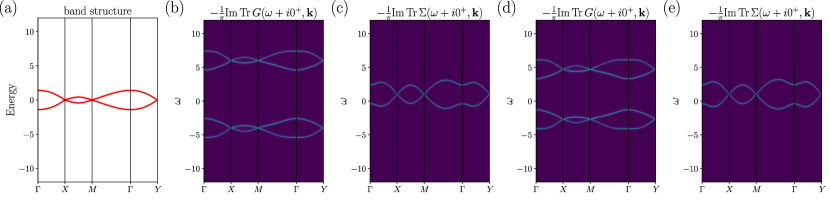
Figure 5: (a) The band structure of the 2D square net lattice with tight binding parameters $t=0.7$ and $t_{SO}=0.42$. (b) The spectral function $A(\omega,\bm{k})=-\frac{1}{\pi}{\rm Im}~{}{\rm Tr}~{}G(\omega+i\delta,\bm{k})$. Here we choose the Hamiltonian parameters as $U_{s}=U_{c}=5$ and $\mu=5$. (c) The imaginary part of the retard self energy $\Sigma(\omega+i\delta,\bm{k})$. A divergent self energy imaginary part indicates a Green’s function zero point. Both the spectral function and self energy are evaluated numerically with exact many-body wavefunctions. In subfigures (d) and (e) we also provide the numerical solution to the spectral function and self energy imaginary part with $V_{03}=V_{30}=0.5$ and $V_{1}^{\prime}=V_{2}^{\prime}=0.2$. Although the dispersion of both zeros and poles of the Green’s function have been changed, the result is qualitatively similar to the analytical solvable case discussed in the main text.

Particle #	States
0	$|0\rangle$
1	$|\uparrow 0\rangle$, $|0\downarrow\rangle$
2	$|\uparrow\downarrow\rangle$

Table 1: List of four possible states with $n=0,1,2$ particles with spin $\sigma$ distributed for a single band with momentum $\bm{k}$.

Particle #	States
0	$|0\rangle$
1	$|\uparrow;0\rangle,|\downarrow;0\rangle,|0;\uparrow\rangle,|0;\downarrow\rangle$
2	$|\uparrow\downarrow;0\rangle,|0;\uparrow\downarrow\rangle,|\uparrow 0;\uparrow 0\rangle$ $|0\downarrow;0\downarrow\rangle,|\uparrow 0;0,\downarrow\rangle,|0\downarrow;\uparrow 0\rangle$
3	$|\uparrow\downarrow;\uparrow 0\rangle,|\uparrow\downarrow;0\downarrow\rangle,|\uparrow 0;\uparrow\downarrow\rangle,|0\downarrow;\uparrow\downarrow\rangle$
4	$|\uparrow\downarrow;\uparrow\downarrow\rangle$

Table 2: List of sixteen possible states with $n=0,..,4$ particles with spin $\sigma$ distributed over two bands with momentum $\bm{k}$. The two bands occupancies are separated by ";".

Appendix B Green’s function

In this section, we outline the formulas leading to the expressions for the total Green’s functions. The time ordered Green’s function is defined in imaginary time by

$$G_{\bm{k}_{1}\sigma_{1}\bm{k}_{2}\sigma_{2}}(\tau) = -\theta(\tau)\langle e^{H\tau}\psi^{\alpha}_{\bm{k}_{1}\sigma_{1}}e^{-H\tau}\psi^{\beta\dagger}_{\bm{k}_{2}\sigma_{2}}\rangle$$ (22)

$$+ \theta(-\tau)\langle\psi^{\alpha\dagger}_{\bm{k}_{2}\sigma_{2}}e^{H\tau}\psi^{\beta}_{\bm{k}_{1}\sigma_{1}}e^{-H\tau}\rangle.$$

The Fourier transform of Green’s function in Matsubara frequency space is given by $G(\tau)=\frac{1}{\beta}\sum_{n}e^{-i\omega_{n}\tau}G(i\omega_{n})$. We can now decompose the propagator in terms of a complete set of eigenstates (listed in Table 2) by inserting identities in the definition of $G_{\bm{k}_{1}\sigma_{1}\bm{k}_{2}\sigma_{2}}(\tau)$. Only same spin and momentum transitions are allowed. This gives us the following expression of the total Green’s function in terms of a complete set of eigenstates

$$\langle e^{H\tau}\psi^{\alpha}_{\bm{k}_{1}\sigma_{1}}e^{-H\tau}\psi^{\beta\dagger}_{\bm{k}_{2}\sigma_{2}}\rangle = \frac{1}{Z}\sum_{\lambda\lambda^{\prime}}e^{-\beta E_{\lambda}}e^{(E_{\lambda}-E_{\lambda^{\prime}})\tau}$$ (23)

$$\langle\lambda|\psi^{\alpha}_{\bm{k}_{1}\sigma_{1}}|\lambda^{\prime}\rangle\langle\lambda^{\prime}|\psi^{\beta\dagger}_{\bm{k}_{2}\sigma_{2}}|\lambda\rangle$$

$$\langle\psi^{\alpha\dagger}_{\bm{k}_{2}\sigma_{2}}e^{H\tau}\psi^{\beta}_{\bm{k}_{1}\sigma_{1}}e^{-H\tau}\rangle = \frac{1}{Z}\sum_{\lambda\lambda^{\prime}}e^{-\beta E_{\lambda}}e^{-(E_{\lambda}-E_{\lambda^{\prime}})\tau}$$ (24)

$$\langle\lambda|\psi^{\alpha\dagger}_{\bm{k}_{2}\sigma_{2}}|\lambda^{\prime}\rangle\langle\lambda^{\prime}|\psi^{\beta}_{\bm{k}_{1}\sigma_{1}}|\lambda\rangle.$$

Here $Z$ is the total partition function. We can then evaluate the total Fourier transformed interacting Green’s function for the first band in the basis of Table 2. When $U^{\prime}\neq 0$, we must evaluate the role of cross terms since we cannot decompose the partition function as a direct product of partition functions for the individual bands. Using the basis in Table 2, the new partition function becomes $Z=\prod_{\bm{k}}Z_{\bm{k}}$ where

$$Z_{\bm{k}} = 1+\sum_{i=1}^{2}\left(2e^{-\beta\xi_{i}}+e^{-\beta(2\xi_{i}+U)}\right)+4e^{-\beta(\xi_{1}+\xi_{2}+U^{\prime})}+2e^{-\beta(2\xi_{1}+\xi_{2}+U+2U^{\prime})}+2e^{-\beta(\xi_{1}+2\xi_{2}+U+2U^{\prime})}+e^{-\beta(2\xi_{1}+2\xi_{2}+2U+4U^{\prime})}.$$

In the expression for $Z_{\bm{k}}$, we have suppressed the momentum argument for convenience of notation. We can then evaluate the total Fourier transformed interacting Green’s function for the first band in the basis of Table 2 as

$$Z_{\bm{k}}G^{(1)}(z) = \frac{1+e^{-\beta\xi_{1}}}{z-\xi_{1}}+e^{-\beta\xi_{1}}\frac{1+e^{-\beta(\xi_{1}+U)}}{z-\xi_{1}-U}+2e^{-\beta\xi_{2}}\frac{1+e^{-\beta(\xi_{1}+U^{\prime})}}{z-\xi_{1}-U^{\prime}}+2e^{-\beta(\xi_{1}+\xi_{2}+U^{\prime})}\frac{1+e^{-\beta(\xi_{1}+U+U^{\prime})}}{z-\xi_{1}-U-U^{\prime}}$$ (25)

$$+e^{-\beta(2\xi_{2}+U)}\frac{1+e^{-\beta(\xi_{1}+2U^{\prime})}}{z-\xi_{1}-2U^{\prime}}+e^{-\beta(\xi_{1}+2\xi_{2}+U+2U^{\prime})}\frac{1+e^{-\beta(\xi_{1}+U+2U^{\prime})}}{z-\xi_{1}-U-2U^{\prime}}.$$

The Green’s function above simplifies in the zero temperature limit where both $\xi_{1}(\bm{k}),\xi_{2}(\bm{k})$ are filled with $U,U^{\prime}>0$. Further when $U+2U^{\prime}>|\xi_{1}|+2|\xi_{2}|,2|\xi_{1}|+|\xi_{2}|$ and $U>2|\xi_{1}|,2|\xi_{2}|$ but $U^{\prime}<|\xi_{1}|+|\xi_{2}|$, the partition function is approximated as $Z_{\bm{k}}\simeq 4e^{-\beta(\xi_{1}+\xi_{2}+U^{\prime})}$. The Green’s function then takes a simple form

$$G^{(1)}(z)=\frac{1}{2}\left[\frac{1}{z-\tilde{\xi}_{1}+U/2-U^{\prime}}+\frac{1}{z-\tilde{\xi}_{1}-U/2-U^{\prime}}\right]$$ (26)

with $\tilde{\xi}_{i}$ being the bare dispersion. Clearly there exist zeros in the Green’s function of band $\tilde{\xi}_{1}(\bm{k})$ when $z=\tilde{\xi}_{1}+U^{\prime}$. The same argument then holds for the second component of the Green’s function, $G^{(2)}(z)$, when $z=\tilde{\xi}_{2}+U^{\prime}$. It is notable that the above derivation for the existence of zeros holds for any $\xi_{1},\xi_{2}$ that satisfy the conditions mentioned above and not specific to Dirac dispersions. In the main text, we use the expressions with $\xi_{1,2}$ replaced by the dispersions of the Young-Kane model.

Appendix C One-band HK Model

The one-band HK Hamiltonian in momentum space contains two terms

$$H=H_{0}+U\sum_{\bm{k}}\left(n_{\bm{k}\uparrow}-\frac{1}{2}\right)\left(n_{\bm{k}\downarrow}-\frac{1}{2}\right),$$ (27)

where $H_{0}$ is the non-interacting piece and is given by $H_{0}=\sum_{\bm{k}\sigma}\xi_{\bm{k}\sigma}c_{\bm{k}\sigma}^{\dagger}c_{\bm{k}\sigma}$. The second term is the interacting piece that is made of density operators $n_{\bm{k}\sigma}=c_{\bm{k}\sigma}^{\dagger}c_{\bm{k}\sigma}$. Here $c_{\bm{k}\sigma}^{\dagger}$ creates an electron in momentum $\bm{k}$ and spin $\sigma$. $U$ is the strength of interaction that is local in momentum space. When Fourier transformed to real space, the interaction term is non-zero only for electrons that satisfy the zero center of mass condition. A noteworthy property of Eq. 27 is the commutativity between the kinetic and interaction terms as well as particle number conservation for each $\bm{k}$. This makes the model analytically tractable in contrast to the Hubbard model. The Hilbert space for each momentum $\bm{k}$ consists of four states shown in Table 1. The partition function for the Hamiltonian Eq. 27 is given by $Z=\prod_{\bm{k}}Z_{\bm{k}}$ where $Z_{\bm{k}}=1+2e^{-\beta\xi_{\bm{k}}}+e^{-\beta(2\xi_{\bm{k}}+U)}$. The exact interacting Green’s function for the single band case is

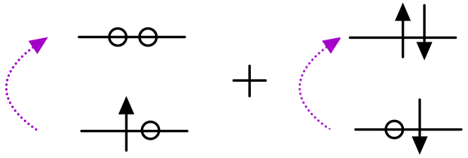
Figure 6: Single band transitions contributing to the interacting Green’s function for a single spin at zero temperature. The circles denote empty states and arrows are pseudo-spin degrees of freedom. The left (right) panel corresponds to electron removal (addition) state. The excitation energies of the two terms are equal and opposite and sum to zero yielding zero surfaces.

$$G_{\sigma}(\bm{k},i\omega_{n})=\frac{1-\langle n_{\bm{k}}\rangle}{i\omega_{n}-\xi_{\bm{k}}-U/2}+\frac{\langle n_{\bm{k}}\rangle}{i\omega_{n}-(\xi_{\bm{k}}-U/2)}.$$ (28)

In the presence of spin-rotation and time reversal invariance, the expression for the Green’s function in Eq. 28 is independent of spin. The expectation value $\langle n_{\bm{k}}\rangle$ is the average occupation of state $\bm{k}$ and is given by

$$\langle n_{\bm{k}}\rangle=\frac{e^{-\beta\xi_{\bm{k}}}+e^{-\beta(2\xi_{\bm{k}}+U)}}{1+2e^{-\beta\xi_{\bm{k}}}+e^{-\beta(2\xi_{\bm{k}}+U)}}.$$ (29)

The limit that is of interest to us is $\beta\rightarrow\infty$ with $\xi_{\bm{k}}<0$ and $U>-\xi_{\bm{k}}$. In this limit, the partition function is $Z=\prod_{\bm{k}}2e^{-\beta\xi_{\bm{k}}}$ and the the occupation number is $\langle n_{\bm{k}}\rangle=\frac{1}{2}$. The Green’s function then reduces to sum of two terms with equal weight of $\frac{1}{2}$ given by

$$G_{\sigma}(\bm{k},i\omega_{n})=\frac{1}{2}\left[\frac{1}{i\omega_{n}-\xi_{\bm{k}}-U/2}+\frac{1}{i\omega_{n}-(\xi_{\bm{k}}-U/2)}\right].$$ (30)

The expression in Eq. 30 shows the existence of poles at $i\omega_{n}=\xi_{\bm{k}}\pm\frac{U}{2}$ which correspond to the lower and upper Hubbard bands. Importantly, when $i\omega_{n}=\xi_{\bm{k}}$, the Green’s function is zero; hence, the original contour of poles of the non-interacting system is converted into a contour of zeros of the interacting Green’s function. The cancellation of transition amplitudes for the single band case is shown in Fig. 6.

Appendix D Spectral degeneracy enforced by non-symmorphic crystalline symmetry

Here we briefly summarize the formulation of the Green’s function based symmetry constraints Hu et al. (2021). This approach starts from expressing the Green’s function as a matrix Abrikosov et al. (2012); Gurarie (2011); Wang et al. (2012). In the space of wavevector $\bm{k}$, frequency $\omega_{n}$ and internal (eg., spin, orbital and sublattice) quantum number $a$,

$$[G]_{(a,i\omega_{n},\bm{k}),(b,i\omega_{m},\bm{k}^{\prime})}=-\langle\psi_{a,i\omega_{n},\bm{k}}\psi^{\dagger}_{b,i\omega_{m},\bm{k}^{\prime}}\rangle\,.$$ (31)

In systems with both space and time translational symmetry, the Green’s functions can be block-diagonalized as Hu et al. (2021)

$$[G]_{(a,i\omega_{m},\bm{k}),(b,i\omega_{n},\bm{k}^{\prime})}=\delta_{mn}\delta_{\bm{k}\bm{k}^{\prime}}[G(i\omega_{n},\bm{k})]_{ab}.$$ (32)

Therefore it is enough to consider the Green’s functions in each block characterized by $(\omega,\bm{k})$. We further do the analytical continuation into the real frequency and define $G(\omega,\bm{k})=G^{R}(\omega,\bm{k})-G^{A}(\omega,\bm{k})$. The matrix $G(\omega,\bm{k})$ is skew-Hermitian and commutes with the symmetry operators. Therefore we have

$$\sum_{b}[G(\omega,\bm{k})]_{ab}[v_{i\omega(\omega,\bm{k})}]_{b}=g_{i}(\omega,\bm{k})[v_{i}(\omega,\bm{k})]_{a}$$ (33)

where $g_{i}(\omega,\bm{k})$ and $[v_{i}(\omega,\bm{k})]_{b}$ are the $i$-th eigenvalues and eigenvectors of each block. At the high symmetry points, the non-symmorphic symmetry further enforces the eigenvectors to form an irrep with a higher dimension Young and Kane (2015). For example, in the case of the 2D square net we considered in the main text, the combination of the time reversal, inversion, and the non-symmorphic glide symmetries enforce the development of the 4d irrep at high symmetry points $X$, $Y$, and $M$. For each $\omega$ at high symmetry points with $\bm{k}=X,Y,M$, the eigenvalues of Green’s function are

$$[G(\omega,\bm{k})]\Gamma^{n}(\omega,\bm{k})=g(\omega,\bm{k})\mathds{1}_{n\times n}\Gamma^{n}(\omega,\bm{k}).$$ (34)

where $\Gamma^{n}$ represents the irrep with dimension $n$. Then, the corresponding spectral functions for each mode in the irrep are identical with

$$\rho(\omega,\bm{k})=-\frac{1}{2\pi}g(\omega,\bm{k}).$$ (35)

Appendix E Matrix-form of the interacting Green’s function

Here we show that the Green’s functions obtained in Eq (6) in the band basis takes the form

$$G(k_{0},\bm{k})=\frac{1}{\tilde{G}^{-1}(k_{0},\bm{k})-(U/2)^{2}\tilde{G}(k_{0},\bm{k})},$$ (36)

in the orbital basis, and discuss its consequences. Here, $k_{0}$ is the Euclidean (equivalently, Matsubara) frequency, and

$$\tilde{G}^{-1}(k_{0},\bm{k})=ik_{0}\mathbbm{1}-\quantity[\vec{n}(\bm{k})\cdot\vec{\Gamma}-(\mu-U^{\prime})\mathbbm{1}]$$ (37)

with $\vec{n}(\bm{k})=\quantity{-t_{SO}\sin{k_{y}},t_{SO}\sin{k_{x}},2t\cos{\frac{k_{x}}{2}}\cos{\frac{k_{y}}{2}}}$, and $\vec{\Gamma}=\tau_{3}\otimes\vec{\sigma}$. The net impact of interactions in (4) of the main text is to shift the chemical potential $\mu\to\mu-U^{\prime}$, and generate the self energy,

$$\Sigma(k_{0},\bm{k})=(U/2)^{2}\tilde{G}(k_{0},\bm{k}).$$ (38)

The poles of $\tilde{G}$ is deduced from the poles of its determinant, which takes the form

$$\det{\tilde{G}}=\frac{1}{\quantity{(k_{0}-i(\mu-U^{\prime}))^{2}+|\vec{n}(\bm{k})|^{2}}^{2}}.$$ (39)

Since $\Sigma\propto\tilde{G}$, the poles of the self-energy are twofold degenerate and are located at

$$k_{0}=i\quantity[(\mu-U^{\prime})\pm|\vec{n}(\bm{k})|].$$ (40)

It is straightforward to be verify that the eigenvalues of $G$ are

$$g_{\pm}(k_{0},\bm{k})=\frac{1}{2}\sum_{s=\pm}\frac{1}{ik_{0}+\mu-U^{\prime}\pm|\vec{n}(\bm{k})|+sU/2},$$ (41)

which implies,

$$\det{G}=\frac{\quantity{(k_{0}-i(\mu-U^{\prime}))^{2}+|\vec{n}(\bm{k})|^{2}}^{2}}{\quantity{(k_{0}-i(\mu-U^{\prime}))^{2}+\quantity(\frac{U}{2}+|\vec{n}(\bm{k})|)^{2}}^{2}\quantity{(k_{0}-i(\mu-U^{\prime}))^{2}+\quantity(\frac{U}{2}-|\vec{n}(\bm{k})|)^{2}}^{2}}.$$ (42)

Since the numerator of $\det{G}$ is precisely equal to the denominator of $\det{\tilde{G}}$, the zeros of $G$ locate exactly at the poles of $\tilde{G}$.

Further, $G$ can be brought to the form,

$$G(k_{0},\bm{k})=iZ_{0}(k)k_{0}\mathbbm{1}+Z_{m}u(k)(\mu-U^{\prime})\mathbbm{1}+Z_{H}(k)\vec{n}(\bm{k})\cdot\vec{\Gamma},$$ (43)

where $Z_{x}$’s are real-valued functions of $(k_{0},\bm{k})$. Since the terms $\propto\mathbbm{1}$ commute with $\Gamma_{j}$, the eigenvectors of $G(k_{0},\bm{k})$ are entirely determined by $\vec{n}(\bm{k})\cdot\vec{\Gamma}$, which is nothing but the single-particle Hamiltonian. Therefore, quite remarkably, the single-particle Hamiltonian and $G$ share the same eigenstates, which are independent of $k_{0}$.

Appendix F Broken time reversal symmetry case

Consider the case when a small Zeeman field with strength $h$ splits the bands of the Dirac semimetal into two Weyl cones. In this case, the modified total partition function $Z=\prod_{\bm{k}}Z_{\bm{k}}(h)$ and Green’s function for the first band are given by

$$Z_{\bm{k}}(h) = 1+e^{-\beta\xi_{1}}+e^{-\beta(\xi_{1}+h)}+e^{-\beta\xi_{2}}+e^{-\beta(\xi_{2}+h)}+e^{-\beta(\xi_{1}+\xi_{2}+U^{\prime})}+2e^{-\beta(\xi_{1}+\xi_{2}+h+U^{\prime})}+e^{-\beta(\xi_{1}+\xi_{2}+2h+U^{\prime})}$$ (44)

$$+ e^{-\beta(2\xi_{1}+h+U)}+e^{-\beta(2\xi_{2}+h+U)}+e^{-\beta(2\xi_{1}+\xi_{2}+U+2U^{\prime}+h)}+e^{-\beta(2\xi_{1}+\xi_{2}+U+2U^{\prime}+2h)}$$

$$+ e^{-\beta(\xi_{1}+2\xi_{2}+U+2U^{\prime}+h)}+e^{-\beta(\xi_{1}+2\xi_{2}+U+2U^{\prime}+2h)}+e^{-\beta(2\xi_{1}+2\xi_{2}+2U+4U^{\prime}+2h)}.$$

$$Z_{\bm{k}}(h)G^{(1)}(z,h) = \frac{1+e^{-\beta\xi_{1}}}{z-\xi_{1}}+e^{-\beta(\xi_{1}+h)}\frac{1+e^{-\beta(\xi_{1}+U)}}{z-\xi_{1}-U}+e^{-\beta\xi_{2}}\frac{1+e^{-\beta(\xi_{1}+U^{\prime})}}{z-\xi_{1}-U^{\prime}}+e^{-\beta(\xi_{2}+h)}\frac{1+e^{-\beta(\xi_{1}+U^{\prime})}}{z-\xi_{1}-U^{\prime}}$$ (45)

$$+ e^{-\beta(\xi_{1}+\xi_{2}+U^{\prime}+h)}\frac{1+e^{-\beta(\xi_{1}+U+U^{\prime})}}{z-\xi_{1}-U-U^{\prime}}+e^{-\beta(\xi_{1}+\xi_{2}+U^{\prime}+2h)}\frac{1+e^{-\beta(\xi_{1}+U+U^{\prime})}}{z-\xi_{1}-U-U^{\prime}}$$

$$+ e^{-\beta(2\xi_{2}+U+h)}\frac{1+e^{-\beta(\xi_{1}+2U^{\prime})}}{z-\xi_{1}-2U^{\prime}}+e^{-\beta(\xi_{1}+2\xi_{2}+U+2U^{\prime}+2h)}\frac{1+e^{-\beta(\xi_{1}+U+2U^{\prime})}}{z-\xi_{1}-U-2U^{\prime}}.$$

Under the assumptions $\xi_{i}(\bm{k}),\xi_{2}(\bm{k})<0$, $U,U^{\prime}>0$, $U+2U^{\prime}>|\xi_{1}|+2|\xi_{2}|,2|\xi_{1}|+|\xi_{2}|$, $U>2|\xi_{1}|,2|\xi_{2}|$ but $U^{\prime}<|\xi_{1}|+|\xi_{2}|$, the dominant processes contributing to the partition function at zero temperature contain purely inter-band interactions. Further assuming that the magnetic field is small and positive, we have $e^{-\beta(\xi_{1}+\xi_{2}+U^{\prime})}\gg e^{-\beta(\xi_{1}+\xi_{2}+h+U^{\prime})}\gg e^{-\beta(\xi_{1}+\xi_{2}+2h+U^{\prime})}$. As a result, the partition function for momentum $\bm{k}$ is approximately $Z_{\bm{k}}\simeq e^{-\beta(\xi_{1}+\xi_{2}+U^{\prime})}$. The Green’s function for the $i$-th band reduces to $G^{(i)}(z)=\frac{1}{z-\xi_{i}-U^{\prime}}$ hence lacking any zeros. Similarly, when $h<0$ we have $e^{-\beta(\xi_{1}+\xi_{2}+U^{\prime})}\ll e^{-\beta(\xi_{1}+\xi_{2}+h+U^{\prime})}\ll e^{-\beta(\xi_{1}+\xi_{2}+2h+U^{\prime})}$. The partition function for momentum $\bm{k}$ is approximately given by $Z_{\bm{k}}\simeq e^{-\beta(\xi_{1}+\xi_{2}+2h+U^{\prime})}$, and the Green’s function reduces to $G^{(i)}(z)=\frac{1}{z-\xi_{i}-U^{\prime}-U}$. We can therefore conclude that broken time reversal automatically destroys any zero surfaces.

Appendix G Spectral crossings on the diamond lattice

On the diamond lattice the undistorted Fu-Kane-Mele model Fu et al. (2007); Fu and Kane (2007) supports Dirac points at the equivalent $X$ points. The model is given by

$$H_{0}(\bm{k})=\sum_{j=1}^{5}d_{j}(\bm{k})\Gamma_{j}$$ (46)

where $\Gamma_{j}=\tau_{3}\otimes\sigma_{j}$, $(\Gamma_{4},\Gamma_{5})=(\tau_{2},\tau_{1})\otimes\sigma_{0}$,

$$d_{1}(\bm{k})=\lambda_{SO}\quantity[\sin{x_{2}}-\sin{x_{3}}-\sin{(x_{2}-x_{1})}+\sin{(x_{3}-x_{1})}]$$

$$d_{2}(\bm{k})=\lambda_{SO}\quantity[\sin{x_{3}}-\sin{x_{1}}-\sin{(x_{3}-x_{2})}+\sin{(x_{1}-x_{2})}]$$

$$d_{3}(\bm{k})=\lambda_{SO}\quantity[\sin{x_{1}}-\sin{x_{2}}-\sin{(x_{1}-x_{3})}+\sin{(x_{2}-x_{3})}]$$

$$d_{4}(\bm{k})=t\quantity[\sin{x_{1}}+\sin{x_{2}}+\sin{x_{3}}]$$

$$d_{5}(\bm{k})=t\quantity[1+\cos{x_{1}}+\cos{x_{2}}+\cos{x_{3}}]$$ (47)

with

$$\quantity(x_{1},x_{2},x_{3})=\quantity(\frac{k_{y}+k_{z}}{2},\frac{k_{x}+k_{z}}{2},\frac{k_{x}+k_{y}}{2}).$$ (48)

When both the $t$ and $t_{SO}$ terms are turned on, the band structure of this tight binding model has a Dirac node at the $X$ point in the first Brillouin zone, which has been shown in Fig. 7(a). Similar to Eq. (Introduction:), we could add a Hatsugai-Kohmoto style interacting Hamiltonian into this model:

$$H =\sum_{\bm{k}}\mathcal{H}_{\bm{k}}\,$$ (49)

$$\mathcal{H}_{\bm{k}} =\Phi^{\dagger}_{\bm{k}}(H_{0}(\bm{k})-\mu\mathbbm{1})\Phi_{\bm{k}}+U_{1}\left(\Phi^{\dagger}_{\bm{k}}\Phi_{\bm{k}}\right)^{2}+U_{2}\left(\Phi^{\dagger}_{\bm{k}}\tau_{3}\otimes\sigma_{3}\Phi_{\bm{k}}\right)^{2}-\frac{U_{1}+U_{2}}{2}\Phi^{\dagger}_{\bm{k}}\Phi_{\bm{k}}\,,$$ (50)

in which $\Phi_{\bm{k}}^{\intercal}=\left(\phi_{1\uparrow\bm{k}},\phi_{1\downarrow\bm{k}},\phi_{2\uparrow\bm{k}},\phi_{2\downarrow\bm{k}}\right)$ represents the spin and orbital basis. Since the interaction is local in the momentum space, we expect the dispersive zeros and poles will exist with a suffiently large $U_{1}$ and $U_{2}$. We choose the values of interaction $U_{1}=U_{2}=5$ and chemical potential $\mu=5$, and numerically solve the Green’s functions of this model. The spectral function and the imaginary part of the self-energy are shown in Fig. 7(b-c), which indicate the dispersion of the poles and zeros of the Green’s function, respectively.

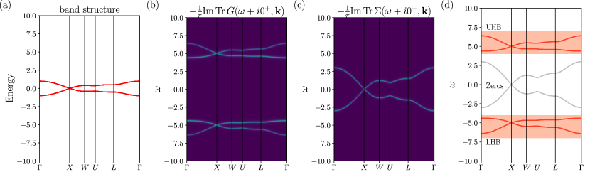
Figure 7: (a) The band structure of the diamond lattice with $t=0.25$ and $\lambda_{SO}=0.1$. (b) The spectral function $A(\omega,\bm{k})$ of the $U_{1}=U_{2}=5$ and $\mu=5$. (c) The imaginary part of the retarded self-energy. (d) Dispersion of the zeros and poles of the Green’s function, and the upper/lower Hubbard bands are labeled by orange shaded regions.

References

• Armitage et al. (2018) N. P. Armitage, E. J. Mele,  and A. Vishwanath, Rev. Mod. Phys. 90, 015001 (2018).
• Nagaosa et al. (2020) N. Nagaosa, T. Morimoto,  and Y. Tokura, Nature Reviews Materials 5, 621 (2020).
• Bradlyn et al. (2017) B. Bradlyn, L. Elcoro, J. Cano, M. G. Vergniory, Z. Wang, C. Felser, M. I. Aroyo,  and B. A. Bernevig, Nature 547, 298 (2017).
• Cano et al. (2018) J. Cano, B. Bradlyn, Z. Wang, L. Elcoro, M. G. Vergniory, C. Felser, M. I. Aroyo,  and B. A. Bernevig, Phys. Rev. B 97, 035139 (2018).
• Po et al. (2017) H. C. Po, A. Vishwanath,  and H. Watanabe, Nature Communications 8, 50 (2017).
• Watanabe et al. (2016) H. Watanabe, H. C. Po, M. P. Zaletel,  and A. Vishwanath, Phys. Rev. Lett. 117, 096404 (2016).
• Cano and Bradlyn (2021) J. Cano and B. Bradlyn, Annu. Rev. Condens. Matter Phys. 12, 225 (2021).
• Son (2007) D. Son, Physical Review B 75, 235423 (2007).
• Sun et al. (2009) K. Sun, H. Yao, E. Fradkin,  and S. A. Kivelson, Physical review letters 103, 046811 (2009).
• Vafek and Yang (2010) O. Vafek and K. Yang, Physical Review B 81, 041401 (2010).
• Herbut et al. (2009) I. F. Herbut, V. Juričić,  and B. Roy, Physical Review B 79, 085116 (2009).
• Sur and Nandkishore (2016) S. Sur and R. Nandkishore, New Journal of Physics 18, 115006 (2016).
• Huh et al. (2016) Y. Huh, E.-G. Moon,  and Y. B. Kim, Physical Review B 93, 035138 (2016).
• Roy (2017) B. Roy, Physical Review B 96, 041113 (2017).
• Sur and Roy (2019) S. Sur and B. Roy, Physical Review Letters 123, 207601 (2019).
• Hu et al. (2021) H. Hu, L. Chen, C. Setty, S. E. Grefe, A. Prokofiev, S. Kirchner, S. Paschen, J. Cano,  and Q. Si, arXiv preprint arXiv:2110.06182  (2021).
• Chen et al. (2022a) L. Chen, C. Setty, H. Hu, M. G. Vergniory, S. E. Grefe, L. Fischer, X. Yan, G. Eguchi, A. Prokofiev, S. Paschen, et al., Nature Physics 18, 1341 (2022a).
• Lai et al. (2018) H.-H. Lai, S. E. Grefe, S. Paschen,  and Q. Si, Proc. Natl. Acad. Sci. U.S.A. 115, 93 (2018).
• Dzsaber et al. (2017) S. Dzsaber, L. Prochaska, A. Sidorenko, G. Eguchi, R. Svagera, M. Waas, A. Prokofiev, Q. Si,  and S. Paschen, Phys. Rev. Lett. 118, 246601 (2017).
• Dzsaber et al. (2021) S. Dzsaber, X. Yan, M. Taupin, G. Eguchi, A. Prokofiev, T. Shiroka, P. Blaha, O. Rubel, S. E. Grefe, H.-H. Lai, Q. Si,  and S. Paschen, PNAS 118, e2013386118 (2021).
• Morimoto and Nagaosa (2016) T. Morimoto and N. Nagaosa, Scientific reports 6, 1 (2016).
• Abrikosov et al. (2012) A. A. Abrikosov, L. P. Gorkov,  and I. E. Dzyaloshinski, Methods of quantum field theory in statistical physics (Courier Corporation, 2012).
• Young and Kane (2015) S. M. Young and C. L. Kane, Physical review letters 115, 126803 (2015).
• Hatsugai and Kohmoto (1992) Y. Hatsugai and M. Kohmoto, Journal of the Physical Society of Japan 61, 2056 (1992).
• Phillips et al. (2018) P. W. Phillips, C. Setty,  and S. Zhang, Physical Review B 97, 195102 (2018).
• Setty (2020) C. Setty, Physical Review B 101, 184506 (2020).
• Setty (2021a) C. Setty, Physical Review B 103, 014501 (2021a).
• Phillips et al. (2020) P. W. Phillips, L. Yeo,  and E. W. Huang, Nature Physics 16, 1175 (2020).
• Huang et al. (2021) E. Huang, G. La Nave,  and P. W. Phillips, arXiv preprint arXiv:2103.03256  (2021).
• Yang (2021) K. Yang, Physical Review B 103, 024529 (2021).
• Zhu et al. (2021) H.-S. Zhu, Z. Li, Q. Han,  and Z. Wang, Physical Review B 103, 024514 (2021).
• Setty (2021b) C. Setty, arXiv preprint arXiv:2105.15205  (2021b).
• Fabrizio (2022) M. Fabrizio, Nature communications 13, 1 (2022).
• Fu et al. (2007) L. Fu, C. L. Kane,  and E. J. Mele, Physical review letters 98, 106803 (2007).
• Fu and Kane (2007) L. Fu and C. L. Kane, Physical Review B 76, 045302 (2007).
• Bradlyn et al. (2016) B. Bradlyn, J. Cano, Z. Wang, M. G. Vergniory, C. Felser, R. J. Cava,  and B. A. Bernevig, Science 353, aaf5037 (2016).
• Di Sante et al. (2017) D. Di Sante, A. Hausoel, P. Barone, J. M. Tomczak, G. Sangiovanni,  and R. Thomale, Phys. Rev. B 96, 121106 (2017).
• Goldoni et al. (1994) A. Goldoni, U. del Pennino, F. Parmigiani, L. Sangaletti,  and A. Revcolevschi, Physical Review B 50, 10435 (1994).
• Garcia-Munoz et al. (1990) J. Garcia-Munoz, J. Rodriguez-Carvajal, F. Sapina, M. Sanchis, R. Ibanez,  and D. Beltran-Porter, Journal of Physics: Condensed Matter 2, 2205 (1990).
• Chen et al. (2022b) L. Chen, F. Xie, S. Sur, H. Hu, S. Paschen, J. Cano,  and Q. Si, arXiv preprint arXiv:2212.08017  (2022b).
• Hu and Si (2022) H. Hu and Q. Si, arXiv preprint arXiv:2209.10396  (2022).
• Gurarie (2011) V. Gurarie, Phys. Rev. B 83, 085426 (2011).
• Wang et al. (2012) Z. Wang, X.-L. Qi,  and S.-C. Zhang, Phys. Rev. B 85, 165126 (2012).