Learning in POMDPs is Sample-Efficient with Hindsight Observability

Abstract

POMDPs capture a broad class of decision making problems, but hardness results suggest that learning is intractable even in simple settings due to the inherent partial observability. However, in many realistic problems, more information is either revealed or can be computed during some point of the learning process. Motivated by diverse applications ranging from robotics to data center scheduling, we formulate a Hindsight Observable Markov Decision Process (HOMDP) as a POMDP where the latent states are revealed to the learner in hindsight and only during training. We introduce new algorithms for the tabular and function approximation settings that are provably sample-efficient with hindsight observability, even in POMDPs that would otherwise be statistically intractable. We give a lower bound showing that the tabular algorithm is optimal in its dependence on latent state and observation cardinalities.

1 Introduction

Sequential decision making settings where the learning agent only receives incomplete observations of its environmental state are typical in diverse practical scenarios, such as control of physical systems (Thrun, 2000), dialogue and recommendation systems (Young et al., 2013; Shani et al., 2005), and decision making in educational or clinical settings (Ayer et al., 2012). Typically studied within the framework of a Partially Observable Markov Decision Process (POMDP), classical literature on such problems provides hardness results on sample and computationally efficient learning, even in simple settings with small action, observation and state spaces, in stark contrast to the MDP setting where the state is fully observable. Fueled by this gap, there is a body of literature that characterizes observability conditions when the sequence of observations reveals enough information about the latent states to permit sample-efficient learning. In this paper, we ask if the motivating practical applications sometimes allow a more informative sensing of the underlying state for some part of the learning process. We formulate a novel learning setting called a Hindsight Observable Markov Decision Process (HOMDP), and provide learning algorithms that are significantly more sample-efficient than those for general POMDPs.

For motivation, let us consider robotic control, where we want our robot to sense its state using a relatively cheap camera sensor upon deployment. However, during training, it is common to allow a more expensive sensing of the state, using simulators, higher-fidelity cameras, lidars, or even full-fledged motion capture setups (Pinto et al., 2017; Pan et al., 2017; Chen et al., 2020). In a completely different style of scenarios, Sinclair et al. (2022) discuss problems such as scheduling in a data center, where the unknown lifetime of a job creates partial observability of the state when the job is scheduled. This partial observability is resolved when the job actually concludes. While the two examples are very different, they share a similarity. The learner needs a decision making policy to act based on partial observations alone, due either to resource/sensor constraints upon deployment or to fundamental lack of information at the time of decision. However, the underlying state eventually gets revealed, either intrinsically, or due to extrinsic measurements during the training process. We refer to this eventual observation of the latent environment state as hindsight observability, and study learning settings where the learner acts based on partial state observations, but observes the true latent states eventually upon the conclusion of the trajectory.

We start by noting that learning in a HOMDP remains considerably challenging in comparison with MDPs, as the learner’s policy needs to depend on observations during deployment (e.g. robotics, scheduling) and sometimes even during training (e.g. scheduling). Hence we cannot use MDP learning techniques directly. At the same time, the HOMDP model eliminates the identifiability or observability conditions that are crucial to success in POMDP learning, since the hindsight observation of the latent state allows us to associate latent states and corresponding observations, albeit with a delay. This makes the HOMDP an intermediate step between the complexity of MDPs and POMDPs, which is practically prevalent as our earlier examples suggest.

Our contributions

In addition to formalizing the HOMDP framework, and showing its broad applicability across diverse settings, such as sim-to-real robotics, high-frequency control, meta-learning and scheduling problems in Appendix A, we make the following key contributions:

1. When the latent states and observations are both finite, we provide an algorithm HOP-B, which finds an $\epsilon$-optimal policy using at most $\widetilde{\mathcal{O}}\left(\frac{XYH^{5}+XAH^{4}}{\epsilon^{2}}\right)$ trajectories, where the HOMDP contains $X$ latent states, $Y$ observations, $A$ actions, and the horizon is $H$. In contrast with standard POMDP learning results, there is no observability-related parameter in our bound.

2. We show an $\Omega(\frac{XY}{\epsilon^{2}})$ lower bound, meaning that HOP-B scales optimally with latent states and observations.

3. We develop a general algorithm, HOP-V, which allows function approximation for both latent states and observations, and allows representation learning in the latent state space. The sample complexity of HOP-V depends on the statistical complexity of function classes used to learn latent state transitions and emissions, along with a rank parameter of the latent state transitions. Again, there are no observability conditions in contrast with standard POMDP results.

2 Related Work

There has been significant progress in understanding the sample efficiency of reinforcement learning in the fully observable setting of MDPs. For tabular MDPs (finite states and actions), upper and lower bounds for sample complexity and regret are well known (Auer et al., 2008; Dann & Brunskill, 2015; Osband & Van Roy, 2016; Azar et al., 2017; Dann et al., 2019; Zanette & Brunskill, 2019). Similar results have been established for MDPs that satisfy certain structural conditions, enabling function approximation (Jiang et al., 2017; Sun et al., 2019; Jin et al., 2020b; Agarwal et al., 2020; Du et al., 2021; Jin et al., 2021a; Foster et al., 2021; Agarwal & Zhang, 2022).

Relative to MDPs, the sample complexity of reinforcement learning in POMDPs is less understood. Classical hardness results suggest learning in POMDPs can be both computationally and statistical intractable even for simple settings (Krishnamurthy et al., 2016). This hardness has spurred researchers to identify conditions under which sample efficient learning is still possible in POMDPs. Block MDPs (Krishnamurthy et al., 2016; Du et al., 2019) and decodable MDPs (Efroni et al., 2022) are special classes of POMDPs in which the current observation (or last few observations) can exactly decode the current latent state. Several works study more general observability conditions beyond decodability (Azizzadenesheli et al., 2016; Guo et al., 2016; Jin et al., 2020a; Golowich et al., 2022; Liu et al., 2022a, b; Uehara et al., 2022). Sample complexity bounds under these conditions often depend crucially on parameters that quantify the degree of observability. Liu et al. (2022b); Zhan et al. (2022); Zhong et al. (2022) provide similar conditions for general predictive state representations (PSRs). Although aimed at the same objective of learning policies for partially observable settings, our work uses hindsight observability to circumvent any additional parameters or assumptions on the emission function.

Empirically, a number of works successfully leverage latent state information during training to improve sample efficiency. Pinto et al. (2017); Baisero & Amato (2021) study asymmetric actor-critic algorithms where the critic uses the latent state while the actor uses observations, allowing the learned policy to later interact with only observations. Pan et al. (2017); Chen et al. (2020); Warrington et al. (2021) use distillation-based approaches where they train an expert policy on latent states and then later imitate it with an observation-based policy. Similar settings also appear as privileged information (Kamienny et al., 2020) or resource-constrained RL (Regatti et al., 2021). However, these prior works do not address sample complexity and exploration.

Motivated by resource allocation, Sinclair et al. (2022) study a similar hindsight problem, where the unobserved part of the latent state is not affected by the learner’s actions, and dynamics are fully known in hindsight. Hence, they study a planning problem in hindsight with no need for exploration, unlike the general HOMDP setting considered here.

Kwon et al. (2021); Zhou et al. (2022) study a latent MDP model, where the latent state contains an additional identifier of the active MDP for each episode, and the identifier is revealed in hindsight during training. Our setting is significantly more general, but shares similar motivation. We compare our bounds in Section 4.

3 Hindsight Observable Markov Decision Process

The underlying model of the HOMDP setting is the same as a POMDP; the difference lies in what information is revealed to the learner and when. We first review the relevant quantities of a POMDP and subsequently introduce the hindsight observability and learning protocol in a HOMDP.

3.1 Preliminaries

For $n\in\mathbb{N}$, we use $[n]$ to denote the set $\{1,2,\ldots,n\}$. For a set $S$, $\Delta(S)$ denotes the set of (appropriately defined) densities over $S$. For $h\in\mathbb{N}$, we use $a_{1:h}$ to denote $(a_{1},\ldots,a_{h})$.

We consider an episodic partially observable Markov decision process (POMDP) $\mathcal{M}$ with episode length $H$, latent state space $\mathcal{X}$, observation space $\mathcal{Y}$, and action space $\mathcal{A}$. When these are finite, we denote their respective cardinalities as $X:=|\mathcal{X}|$, $Y:=|\mathcal{Y}|$, and $A:=|\mathcal{A}|$. An initial latent state $x_{1}$ is sampled from a fixed and known initial state distribution $\rho\in\Delta(\mathcal{X})$. The process evolves according to transition function $T_{\star}:\mathcal{X}\times\mathcal{A}\to\Delta(\mathcal{X})$, acting on the latent states. When the learner visits a latent state $x$, the environment generates an observation $y\in\mathcal{Y}$ according to the conditional emission function $O_{\star}:\mathcal{X}\to\Delta(\mathcal{Y})$. In particular, in each episode, a (latent) trajectory $\bar{\tau}=(x_{1},y_{1},a_{1},\ldots,x_{H},y_{H},a_{H},x_{H+1})$ is generated where $x_{1}\sim\rho(\cdot)$, $x_{h+1}\sim T_{\star}(\cdot|x_{h},a_{h})$, $y_{h}\sim O_{\star}(\cdot|x_{h})$, and the learner selects $a_{1:H}$. We include $x_{H+1}$ (from taking $a_{H}$ in $x_{H}$) as a latent variable for convenience. When referring to an (observed) trajectory of just observations and actions, we use $\tau=(y_{1},a_{1},\ldots,y_{H},a_{H})$. We assume there is a known deterministic reward function $r:\mathcal{X}\times\mathcal{A}\to[0,1]$. Our results can be generalized readily to stochastic, observation-dependent rewards.

As is standard in POMDPs, we consider the setting where the learner interacts with the environment by specifying a history-dependent policy $\pi\ :\ (\mathcal{Y}\times\mathcal{A})^{*}\times\mathcal{Y}\to\Delta(\mathcal{A})$ which takes as input a (variable) $h$-length history of observations $y_{1:h}$ and $(h-1)$-length history of actions $a_{1:h-1}$ and outputs a distribution over actions. That is, the learner’s policy does not get to observe any of the latent states $x_{1:H+1}$ during execution of $\pi$. For conciseness, we denote the partial histories as $\tau_{h}:=(y_{1:h},a_{1:h-1})$ and $\bar{\tau}_{h}:=(y_{1:h},x_{1:h},a_{1:h-1})$, which includes the observation $y_{h}$ and latent state $x_{h}$ (if applicable) at step $h$.

For a policy $\pi$, we denote the expected cumulative reward over an episode by

$$v(\pi)=\mathbb{E}_{\pi}\left[\sum_{h\in[H]}r(x_{h},a_{h})\right],$$ (1)

where $\mathbb{E}_{\pi}$ is the expectation taken over trajectories in the POMDP under policy $\pi$.

3.2 Hindsight observability

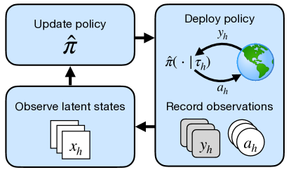
Figure 1: A HOMDP model at train time. The learned history-dependent policy $\hat{\pi}$ is deployed and takes actions $a_{1:H}$ using only observations $y_{1:H}$. After deployment, the environment reveals the latent states $x_{1:H+1}$. The policy updates with both the latent states $x_{1:H+1}$ and observations $(y_{1:H},a_{1:H})$. At test time, only a history-dependent policy is deployed.

Now we formally introduce the HOMDP setting and describe the interaction protocol, i.e., how the learner interacts with the environment and receives information. We also illustrate this description in the accompanying Figure 1. Along the way, we highlight differences with the standard POMDP and MDP settings. There are two phases in the HOMDP: train time and test time.

During train time, the learner interacts with the environment over $K\in\mathbb{N}$ rounds (episodes). At any given round $k\in[K]$, the learner produces a history-dependent policy $\hat{\pi}_{k}$ which is deployed in the partially observable environment as if the learner is interacting with a standard POMDP. During execution of the episode $k$ at time $h\in[H]$, the environment reveals only the current observation $y_{h}$ to the learner. The policy can thus base its decision $a_{h}$ on only the partial history $\tau_{h}=(y_{1:h},a_{1:h-1})$ of interactions in that episode. Once the $k$th episode is completed, the latent states $x_{1:H+1}$ are revealed to the learner in hindsight, hence the terminology hindsight observability. The learner can then generate a new policy $\hat{\pi}_{k+1}$ using information from $(x_{1:H+1},y_{1:H},a_{1:H})$ as well as that of all previous episodes. This is the key difference between HOMDPs and standard POMDPs where the latent states are never revealed and the learner generates the policy from only previous observations, actions, and rewards alone. In MDPs, on the other hand, the latent state is observed instantaneously and the policy can directly map a latent state to an action.

The train time phase may be followed by a test time phase where a single history-dependent policy $\hat{\pi}$ is deployed but the learner does not observe latent states or update the policy after committing to $\hat{\pi}$. To determine $\hat{\pi}$, the learner can use all of the information collected over the $K$ episodes at train time, including the latent states observed in hindsight. The quantity $v(\hat{\pi})$ evaluates the quality of $\hat{\pi}$. We let $\pi^{\star}$ denote the optimal observation-based policy maximizing $v(\pi^{\star})$ and measure the sub-optimality of the learner’s policy $\hat{\pi}$ by the difference $v(\pi^{\star})-v(\hat{\pi})$. Again, in contrast with an MDP, a HOMDP never reveals the latent state at test time.

We are primarily concerned with PAC sample complexity bounds controlling the suboptimality of $\hat{\pi}$, but some algorithms also address the regret problem at train time where the regret for all $K$ rounds is measured as

$$\operatorname{Reg}(K)=\sum_{k\in[K]}v(\pi^{\star})-v(\hat{\pi}_{k}).$$

Example 1 (Sim-to-real robotics).

In sim-to-real robotics (Pinto et al., 2017), one trains an image-based policy in a simulator with access to the underlying states. The goal is to deploy the image-based policy in the real world. $\mathcal{X}$ is the set of robot and object positions and poses which are observable in the simulator during training. $\mathcal{Y}$ is the set of image observations from a camera, which is the only modality available at test time. $\mathcal{X}$ and $\mathcal{Y}$ are both continuous and high dimensional. $\mathcal{A}$ is the set of control inputs the robot can take such as joint torques. Note that the latent states are available without delay at train time in this example. However, we later show that this variant of the problem interestingly does not yield significant statistical advantage in theory because the desired policy at test time is still history-dependent (see the discussion following Theorem 5.1). Empirically, history-dependent policies are still preferred to state-based policies even during train time despite access to the state to facilitate better sim-to-real transfer.

Example 2 (Data center scheduling).

In data center scheduling (Sinclair et al., 2022), described in the introduction, $\mathcal{Y}$ is the observable state of the submitted, processing, and completed jobs as well as their allocations to servers, which is available at the time of decision-making. $\mathcal{X}$ is a concatenation of $\mathcal{Y}$ with lifetime lengths of the submitted/processing jobs and the arrival times of future jobs. This information is available, but only in hindsight. Depending on the setup, $\mathcal{X}$ and $\mathcal{Y}$ can be relatively succinct here. $\mathcal{A}$ is the set of allocation actions for currently submitted jobs.

3.3 Comparison with hardness of learning in POMDPs

Both POMDPs and HOMDPs share the use of history-dependent policies during execution at test time. However, a POMDP never reveals the association between observations and latent states, leading to a lack of identifiability and exponential in $H$ lower bounds even for simple ones (Krishnamurthy et al., 2016). As discussed previously, numerous recent papers (Liu et al., 2022a; Jin et al., 2020a; Cai et al., 2022; Liu et al., 2022b; Zhan et al., 2022) investigate observability conditions under which sample-efficient learning is possible by ensuring $O_{\star}$ reveals enough about the distribution of possible latent states. This yields sample complexity bounds that incur an unavoidable dependence on the minimum singular value of $O_{\star}$ (Liu et al., 2022a), or related parameters.

However, settings where such observability conditions are satisfied may still preclude many practically interesting partially observable problems. Our objective in this paper is to understand to what extent the addition of hindsight observability in a HOMDP can make learning in partially observable settings sample-efficient without relying on observability parameters.

4 Learning in Finite HOMDPs

We now turn to the design of efficient algorithms for learning in the HOMDP model. We begin with the setting where the latent state space $\mathcal{X}$ and observation space $\mathcal{Y}$ have finite cardinalities $X:=|\mathcal{X}|$ and $Y:=|\mathcal{Y}|$. We introduce a new algorithm, HOP-B, which naturally extends minimax optimal results (in $X$ and $A$) for tabular MDPs to the HOMDP model. Our proposed algorithm is model-based, leveraging the intuition that, provided with the latent states $x_{1:H+1}$, one should be able to estimate the transition and emission functions, $T_{\star}$ and $O_{\star}$. We start with the algorithm, before presenting the sample complexity guarantee.

4.1 The HOP-B algorithm

Our algorithm, Hindsight OPtimism with Bonus (HOP-B) estimates the transition and emission models, and subsequently finds an optimal policy in this learned model using a reward bonus to encourage exploration. The design of bonus is a key novelty in HOP-B, relative to its MDP counterparts, as we will discuss shortly.

Before describing the algorithm, we define a planning oracle which is used in the algorithm to compute the exploration policies. Note that planning in a HOMDP is identical to a POMDP, as we seek an optimal history-dependent policy.

Definition 4.1 (Optimal planner).

The POMDP planner POP takes as input a transition function $T$, an emission function $O$, and a reward function $r$ and returns a policy $\pi=\textsf{POP}(T,O,r)$ such that $v(\pi)=\max_{\pi^{\prime}}v_{\mathcal{M}(T,O,r)}(\pi^{\prime})$, where $\mathcal{M}(T,O,r)$ denotes the POMDP model with latent transitions $T$, emissions $O$, and reward function $r$.

While it is known that planning in POMDPs is PSPACE-hard in general (Papadimitriou & Tsitsiklis, 1987), there are many special classes of POMDPs for which planning is computationally efficient. Alternatively, it is possible in practice to use one of many existing approximate POMDP planners; however, this will likely weaken the subsequent theoretical guarantees of this section up to some approximation error. Regardless, this is much milder computational assumption than what is sometimes made in comparable POMDP literature (Jin et al., 2020a).

Algorithm 1 Hindsight OPtimism with Bonus (HOP-B)

1:  Input: POMDP planner POP.

2:  Initialize emission and transition models $\hat{O}_{1},\hat{T}_{1}$.

3:  Initialize $n_{1}(x)=n_{1}(x,a)=0$ for all $x\in\mathcal{X},a\in\mathcal{A}$.

4:  Set bonus parameters$\beta_{1}=4H^{3}\log(YXAHK/\delta),\beta_{2}=8Y\log(YXKH/\delta).$

5:  for  $k=1,\ldots,K$  do

6:     // Set reward bonuses

7:     $\epsilon_{k}(x,a)=\min\left\{\sqrt{\beta_{1}\over n_{k}(x,a)},2H\right\}$

8:     $\epsilon_{k}(x)=\min\left\{\sqrt{\beta_{2}\over n_{k}(x)},2\right\}$

9:     $\hat{r}_{k}(x,a)=r(x,a)+H\epsilon_{k}(x)+\epsilon_{k}(x,a)$

10:     // Plan, deploy hist.-dependent policy

11:     $\hat{\pi}_{k}=\textsf{POP}(\hat{T}_{k},\hat{O}_{k},\hat{r}_{k})$

12:     Run $\hat{\pi}_{k}$ and observe trajectory $\tau^{k}=(y_{1:H}^{k},a_{1:H}^{k})$.

13:     // Hindsight observation

14:     Observe latent states $x^{k}_{1:H+1}=(x^{k}_{1},\dots,x^{k}_{H+1})$.

15:     // Update models

16:     $n_{k+1}(x)=\sum_{\ell\in[k],h\in[H]}\mathbf{1}\{x^{\ell}_{h}=x\}$.

17:     $n_{k+1}(x,a)=\sum_{\ell\in[k],h\in[H]}\mathbf{1}\{x^{\ell}_{h}=x\wedge a^{\ell}_{h}=a\}$.

18:     Update $\hat{T}_{k+1}$ via (2)

19:     Update $\hat{O}_{k+1}$ via (3)

20:  end for

HOP-B operates over $K$ rounds, starting with arbitrary guesses $\hat{T}_{1}$ and $\hat{O}_{1}$ of the model. At round $k$, it computes reward bonuses based on the uncertainty in the estimates $\hat{T}_{k}$ and $\hat{O}_{k}$, which is quantified by the number of visits to each latent state $x$ and latent-state action pair $(x,a)$ from the dataset. We define these bonuses in $\epsilon_{k}(x)$ and $\epsilon_{k}(x,a)$ in lines 7 and 8 with parameters given in line 4. Note that the $\epsilon_{k}(x)$ bonus is in addition to the typical bonus in MDPs. Informally $\epsilon_{k}(x,a)$ captures our uncertainty in the estimation of $T_{\star}$, while $\epsilon_{k}(x)$ measures it for $O_{\star}$. For instance, even if we know $T_{\star}$, we need to visit each latent state to estimate its emission process for the subsequent planning, capturing the need for the additional $\epsilon_{k}(x)$ bonus.

We construct a reward function $\hat{r}_{k}$ by adding the bonuses to $r$. We then invoke the planner POP using $\hat{T}_{k}$, $\hat{O}_{k}$, and the reward function $\hat{r}_{k}$ to generate an optimistic history-dependent policy $\hat{\pi}_{k}$. As we show in the proof, the estimated value of $\hat{\pi}_{k}$ under the current model over-estimates the true value of $\pi^{\star}$ with high probability. We then deploy the optimistic policy $\hat{\pi}_{k}$ in the environment to generate a trajectory of observations $y_{1:H}$ and actions $a_{1:H}$. We further observe the latent states $x_{1:H+1}$ in hindsight. Finally, using the new information from the trajectory and in hindsight, we update the models with empirical estimates using all the past data:

(2)

$$\hskip 8.53581pt\hat{O}_{k+1}(y|x)=\sum_{\ell\in[k],h\in[H]}{\mathbf{1}\left\{x^{\ell}_{h}=x,y^{\ell}_{h}=y\right\}\over n_{k+1}(x)}$$ (3)

for all $x,x^{\prime},a,y$ where $n_{k+1}(x,a)$ and $n_{k+1}(x)$ are defined in Algorithm 1. Note that both the calculation of the uncertainty bonuses and the model updates are possible only due to the hindsight observability that reveals the latent states $x^{\ell}_{1:H+1}$ for $\ell\in[k-1]$. In general POMDPs, such calculations are not available.

4.2 Regret and sample complexity bounds

We now present the main guarantees for HOP-B in HOMDPs. While we are primarily concerned with sample complexity bounds, HOP-B readily admits a regret bound.

Theorem 4.2.

Let $\mathcal{M}$ be a HOMDP model with $X$ latent states and $Y$ observations. With probability at least $1-\delta$, HOP-B outputs a sequence of policies $\hat{\pi}_{1},\ldots,\hat{\pi}_{K}$ such that

$$\operatorname{Reg}(K)=\widetilde{\mathcal{O}}\left(\sqrt{{(XYH^{5}+XAH^{4})K\iota}}\right),$$

where $\iota=\log({2X^{2}YAKH}\delta^{-1})$ and $\widetilde{\mathcal{O}}$ omits lower-order terms in $K$.

The full bound, including lower order terms, and the proof can be found in Appendix C. A standard online-to-batch conversion reveals that HOP-B learns an $\epsilon$-optimal policy at test time with probability at least $1-\delta$ with sample complexity

$$K=\widetilde{\mathcal{O}}\left({XYH^{5}+XAH^{4}\over\epsilon^{2}}\right),$$

omitting log factors and lower-order terms in $\epsilon$. We highlight several conceptual implications of the results.

• The bounds do not have dependence on any observability parameter, which typically measures the degree to which one can decode the latent distribution from observations in POMDPs. For instance, guarantees of Liu et al. (2022a) depend polynomially on the inverse of the minimum singular value of $O_{\star}$ and in fact this dependence is necessary in general POMDPs (see e.g. Theorem 6 in Liu et al., 2022a). This precludes efficient learning in a wide class of partially observed problems (such as vision-based robotics applications with occlusions). By leveraging hindsight observability, our results show that it is possible to circumvent this hardness while still learning a near optimal history-dependent policy for test time.

• The leading terms depend linearly on the number of observations $Y$ and latent states $X$. Inspecting just the dependence in $X$ and $A$, the result of Theorem 4.2 can thus be viewed as a natural extension of minimax regret (and sample complexity) results for the MDPs. This is known to be unimprovable in general even for full information MDPs (Dann & Brunskill, 2015; Osband & Van Roy, 2016). However, due to the added complexity of partial observability during deployment, a linear term in $Y$ is also present our bound. Our lower bound in Theorem 5.1 shows that the linear $XY$ dependence is minimax optimal. We remark prior work on POMDPs has yielded large polynomial dependence on $X$ and $Y$ in contrast to our linear dependence here.

• An interesting observation of HOP-B is that the exploration bonus need only happen at the latent state level, rather than needing to explore histories. This suggests that little structure might be needed to learn $O_{\star}$. We will see in Section 6 that this observation becomes deeper when incorporating function approximation.

The dependence on the horizon $H$, although still polynomial, is likely suboptimal; however, we conjecture that it can be improved using known tools for MDPs. Since our focus is on the impact of $X$ and $Y$ and understanding the fundamental efficiency gaps between HOMDPs and POMDPs, we leave optimizing these additional factors for future work. As discussed before, HOMDPs are a generalization of latent MDPs with identifiers labeled in hindsight studied by Kwon et al. (2021); Zhou et al. (2022). Ignoring $H$ and specializing our bound to their setting, it matches Kwon et al. (2021). Zhou et al. (2022) is better by a sparsity factor, but is more specialized and not applicable to general HOMDPs.

Proof intuition.

HOP-B resembles typical optimistic algorithms for MDPs. However, a naïve analysis by computing confidence intervals on $\hat{T}_{k}-T_{\star}$ and $\hat{O}_{k}-O_{\star}$ results in an $\mathcal{O}(X^{2})$ scaling of sample complexity. We follow the MDP literature in constructing more careful confidence bounds on appropriate value functions instead. This requires some care as value functions are history-dependent in a HOMDP. In particular, we need to control the required exploration as a function of latent state visitations, while reasoning over history-dependent value functions. Combining these ideas carefully, which we present in detail in Appendix C, gives the proof of Theorem 4.2. We note that most POMDP analyses do suffer from the $\mathcal{O}(X^{2})$ or worse scaling, as they do not reason via value functions.

5 Limits of Learning in Tabular HOMDPs

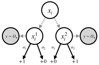
Figure 2: Simplified case of the lower bound construction. The learner starts in $x_{i}$ and randomly transitions to $x_{i}^{1}$ or $x_{i}^{2}$. The optimal action to achieve reward $+1$ is different depending on which latent state is visited, but the observation $y$ obfuscates sensing of the latent state.

We now show that the upper bound of the previous section is optimal in $XY$ for the tabular setting. We present a new information-theoretic lower bound for the tabular HOMDP setting. The proof is in Appendix D.

Theorem 5.1.

Fix $\epsilon\leq 1/64$ and $X,Y\in\mathbb{N}$ such that $Y\geq 6$, $(X+1)\geq 128\log 2$. For any algorithm $\mathfrak{A}$ producing a policy $\hat{\pi}$ in $K$ episodes of interaction, there exists a HOMDP with the aforementioned cardinalities and $H\asymp\log_{2}(X)$ and $A=2$ such that $\mathfrak{A}$ needs

$$K=\Omega\left({XY/\epsilon^{2}}\right)$$

to guarantee $\mathbb{E}\left[v(\pi^{\star})-v(\hat{\pi})\right]\leq\epsilon$, where the expectation is taken over randomness in the data and algorithm.

The lower bound is information-theoretic, meaning that no algorithm can do better than this. The lower bound of Theorem 5.1 matches the $XY$ leading term of the upper bound in Theorem 4.2, suggesting that our algorithm is minimax optimal in $X$ and $Y$ for large $K$. Recall that existing lower bounds for learning in MDPs necessitate $\Omega\left(\nicefrac{{XA}}{{\epsilon^{2}}}\right)$ episodes of interaction, which accounts for the other leading term in our upper bound (Dann & Brunskill, 2015; Osband & Van Roy, 2016). Since POMDPs are more general than HOMDPs, our lower bound also applies to POMDPs.

Hindsight vs. foresight observability. Our lower bound construction does not distinguish between the latent state $x_{h}$ being simultaneously revealed along with $y_{h}$, or only in hindsight. The key bottleneck is in the construction of the history-dependent policy at test time. Therefore, revealing states simultaneously is no easier statistically than revealing them in hindsight, at least in a minimax sense. This lends credence to framing a broader class of problems such as sim-to-real robotics as HOMDPs by dealing with latent states after execution of a policy even though the state is always observable during training. Because one seeks a history-dependent policy in the end, it is just as hard statistically.

Intuition for lower bound construction.

We derive the lower bound by constucting a class of hard HOMDP models in the form a binary tree for the latent states, like many hard MDP constructions. At the final layers of the tree is a collection of $\Omega(X)$ subproblems, each of the form of Figure 2. In each subproblem there are $3$ latent states. The learner starts in $x_{i}$ and transitions randomly to either of the child states $x_{i}^{1}$ and $x_{i}^{2}$ with equal probability and must take an optimal action that depends on which one it visits. The difficulty is that $O_{\star}$ is biased slightly towards half of the observations depending on the latent state. As a result, in order to effectively match the value of the optimal policy, the learner must interact at least $\Omega(Y)$ times with this subproblem. To prove there is linear dependence on $XY$, we leverage the binary tree described earlier. In short, the learner transitions randomly down the tree until it reaches one of $\Omega(X)$ independent subproblems (decodable from the observations), where it must play optimally. As we remarked earlier, the bottleneck is on the history-dependent policy deployed at test-time, so observing the latent states simultaneously at training does not help in solving this construction.

6 Generalization in HOMDPs

While the tabular setting considered so far is important for building intuition, and tabular latent states are particularly reasonable in many settings, several practical domains of interest necessitate continuous and high-dimensional latent states and observations. In this section, we study HOMDPs where both $\mathcal{X}$ and $\mathcal{Y}$ can be infinitely large, and we employ function approximation for sample-efficient learning. Mirroring prior work in MDPs and more recently POMDPs, this requires structural conditions on the underlying latent state transitions $T_{\star}$. We now describe one such condition which has been widely studied in the MDP literature, and present an algorithm and sample complexity guarantees.

6.1 Low-rank latent transition dynamics

We initiate this investigation with a well-studied model in the MDP literature: the low-rank MDP (Barreto et al., 2011; Jiang et al., 2017; Agarwal et al., 2020). We study HOMDPs where the underlying latent state MDP is low-rank.

Definition 6.1.

A transition function $T_{\star}$ admits a low-rank decomposition with rank $d$ if there exist vector functions $\phi_{\star}:\mathcal{X}\times\mathcal{A}\to\mathbb{R}^{d}$ and $\psi_{\star}:\mathcal{X}\to\mathbb{R}^{d}$ such that

$$T_{\star}(x^{\prime}|x,a)=\phi_{\star}(x,a)^{\top}\psi_{\star}(x^{\prime})\quad\forall x,x^{\prime}\in\mathcal{X},a\in\mathcal{A}$$

Furthermore, $\phi_{\star}$ satisfies $\sup_{x,a}\|\phi_{\star}(x,a)\|_{2}\leq 1$ and $\psi_{\star}$ satisfies $\|\int_{x^{\prime}}\psi_{\star}(x^{\prime})\mathop{}\!\mathrm{d}x^{\prime}\|_{2}\leq\sqrt{d}$.

Note that in the low-rank setting, we do not assume that the feature embedding $\phi_{\star}$ is known, unlike the linear MDP setting (Jin et al., 2020b) which crucially leverages this knowledge. We defer details, motivations, and comparisons to the original papers on the matter (Agarwal et al., 2020).

We assume that the learner has access to function classes $\mathcal{T}$ and $\Theta$ for approximation of $T_{\star}$ and $O_{\star}$, respectively. For simplicity of the analysis, we assume that they are finite but large, and thus we desire a sample complexity which is logarithmic in $|\mathcal{T}|$ and $|\Theta|$, with no explicit dependence on $|\mathcal{X}|$ or $|\mathcal{Y}|$. This formulation also automatically captures the representation learning problem for the latent states (Agarwal et al., 2020). As is standard, we assume that the function classes are proper and satisfy realizability.

Assumption 6.2.

$T_{\star}\in\mathcal{T}$ and $O_{\star}\in\Theta$. Furthermore, for all $T\in\mathcal{T}$ and $O\in\Theta$, $T(\cdot|x,a)\in\Delta(\mathcal{X})$ and $O(\cdot|x,a)\in\Delta(\mathcal{Y})$ for all $x,x^{\prime}\in\mathcal{X}$ and $a\in\mathcal{A}$.

The above requires that all candidates in the class can form valid distributions (i.e., they are proper); this can be satisfied by simply discarding those in $\mathcal{T}$ and $\Theta$ that are improper.

6.2 The HOP-V algorithm

Algorithm 2 ​Hindsight OPtimism with Version spaces ​(HOP-V)

1:  Input: Transition class $\mathcal{T}$, Emission class $\Theta$.

2:  Set $K^{\prime}=\lfloor K/H\rfloor$.

3:  Set $\beta_{\mathcal{T}}=2\log\left(K^{\prime}|\mathcal{T}|/\delta\right)$.

4:  Set $\beta_{\Theta}=2\log\left(K^{\prime}|\Theta|/\delta\right)$.

5:  Initialize $\mathcal{T}_{1}=\mathcal{T}$. and $\Theta_{1}=\Theta$.

6:  for  $k=1,\ldots,K^{\prime}$  do

7:     // Optimistic planning

8:     Solve

$$\hat{\pi}_{k},\hat{O}_{k},\hat{T}_{k}=\operatorname*{arg\,max}_{\pi\in\Pi,T\in\mathcal{T}_{k},O\in\Theta_{k}}v_{\mathcal{M}(T,O)}(\pi)$$

9:     for  $h\in[H]$  do

10:        // Deploy hist.-dependent policy

11:        Construct exploration policy $\tilde{\pi}_{k}=\hat{\pi}_{k}\circ_{h}\operatorname*{Unif}(\mathcal{A})$

12:        Deploy $\tilde{\pi}_{k}$ and observe trajectory $(y_{1:H},a_{1:H})$. // Hindsight observation

13:        Observe latent states $x_{1:H+1}$.

14:        Set $y^{k}_{h}:=y_{h}$, $a^{k}_{h}:=a_{h}$, $x^{k}_{h}:=x_{h}$, $\tilde{x}^{k}_{h}:=x_{h+1}$.

15:     end for

16:     Update version spaces with

$$\mathcal{T}_{k+1} =\left\{T\in\mathcal{T}_{k}\ :\ \hat{\mathcal{L}}^{1}_{k}(T)\geq\max_{T^{\prime}\in\mathcal{T}_{k}}\hat{\mathcal{L}}^{1}_{k}(T^{\prime})-\beta_{\mathcal{T}}\right\}$$

$$\Theta_{k+1} =\left\{O\in\Theta_{k}\ :\ \hat{\mathcal{L}}^{2}_{k}(O)\geq\max_{O^{\prime}\in\Theta_{k}}\hat{\mathcal{L}}^{2}_{k}(O^{\prime})-\beta_{\Theta}\right\}$$

17:  end for

We now introduce the algorithm Hindsight OPtimism with Version spaces (HOP-V) for function approximation in HOMDP models. HOP-V divides the $K$ rounds into $K^{\prime}=\lfloor K/H\rfloor$ epochs and maintains version spaces $\mathcal{T}_{k}$ and $\Theta_{k}$ over the model classes based on the data collected so far for each epoch $k\in[K^{\prime}]$. In epoch $k$, HOP-V identifies a policy $\hat{\pi}_{k}$ and models $\hat{T}_{k}$ and $\hat{O}_{k}$ by solving an optimistic optimization problem over the version spaces. Here $v_{\mathcal{M}(T,O)}(\pi)$ denotes the value of a policy $\pi$ in the POMDP model given by transition function $T$, emission function $O$ and the true reward function $r$, akin to the original definition in (1). Still within epoch $k$, for each $h\in[H]$, HOP-V generates an exploration policy from $\hat{\pi}_{k}$ by taking $\tilde{\pi}_{k}=\hat{\pi}_{k}\circ_{h}\operatorname*{Unif}(\mathcal{A})$. The operator $\circ_{h}$ replaces $\hat{\pi}(\cdot|\tau_{h})$ with the uniform distribution $\operatorname*{Unif}(\mathcal{A})\in\Delta(\mathcal{A})$ over the actions for all $h$-length histories $\tau_{h}$, but leaves the rest of $\hat{\pi}_{k}$ unaffected. That is, $\tilde{\pi}_{k}$ plays $\hat{\pi}_{k}$ normally up to the $h$th step and then takes a random action.

HOP-V deploys the exploration policy $\tilde{\pi}_{k}$ in the environment and records the observation $y_{h}^{k}$ and action $a_{h}^{k}$. Then, when the latent states are revealed, it records the latent state $x_{h}^{k}$ and the next state ${\tilde{x}_{h}^{k}}$. It repeats this exploration procedure for each $h\in[H]$ in the epoch $k$ to generate $(y_{1:H}^{k},a_{1:H}^{k},x_{1:H}^{k},\tilde{x}_{1:H}^{k})$. Based on this new data, it updates the version spaces via maximum likelihood estimation (MLE) with the following log-likelihood objectives:

$$\hat{\mathcal{L}}_{k}^{1}(T) =\sum_{\ell\in[k],h\in[H]}\log T(\tilde{x}^{\ell}_{h}|x^{\ell}_{h},a^{\ell}_{h})\quad\text{and}$$

$$\hat{\mathcal{L}}_{k}^{2}(O) =\sum_{\ell\in[k],h\in[H]}\log O(y_{h}^{\ell}|x_{h}^{\ell}).$$

6.3 Sample complexity bound

We now state the performance guarantee for HOP-V.

Theorem 6.3.

Let $\mathcal{M}$ be a HOMDP model with a low-rank transition function $T_{\star}$ of rank $d$. Let $\mathcal{T}$ and $\Theta$ satisfy Assumption 6.2. Then, with probability at least $1-\delta$, HOP-V outputs a sequence of policies $\hat{\pi}_{1},\ldots,\hat{\pi}_{K^{\prime}}$ such that

$$\operatorname{Reg}(K^{\prime})=\mathcal{O}\left(\sqrt{{AH^{4}dK^{\prime}}\log\left(K^{\prime}H|\Theta||\mathcal{T}|\over\delta\right)\log K^{\prime}}\right)$$

Note that the regret is over the learned $\hat{\pi}_{1:K^{\prime}}$, not the actually deployed exploration policies. This phenomenon occurs often from one-step exploration (Jiang et al., 2017; Agarwal et al., 2020). However, our focus is the implied PAC guarantee. Again, using a standard online to batch conversion, we get that HOP-V learns an $\epsilon$-optimal policy with probability at least $1-\delta$ in

$$K=\widetilde{\mathcal{O}}\left({AH^{5}d\over\epsilon^{2}}\log\left({|\Theta||\mathcal{T}|\over\delta}\right)\right)$$

episodes of interaction. The additional $H$ arises because there are $H$ episodes for each epoch $k\in[K^{\prime}]$ due to the construction and deployment of the exploration policies.

• In contrast to the tabular bound of HOP-B, HOP-V has no dependence on the size of the latent state space $X$ or observation space $Y$. Instead, generalization using function classes replaces them with complexities of $\mathcal{T}$ and $\Theta$ and the rank $d$ of the latent transition. Note that we can readily replace these log-cardinalities with other suitable notions of complexity for infinite function classes.

• For comparison to Theorem 4.2, we can set $d=X$, $\log|\Theta|=\widetilde{\mathcal{O}}(XY)$ and $\log|\mathcal{T}|=\widetilde{\mathcal{O}}(X^{2}A)$, which results in a suboptimal scaling in $X$ as HOP-V does not use value function-based optimism unlike HOP-B.

• Similar to the tabular setting, the sample complexity also has no dependence on observability parameters, showing that we maintain this advantageous property of HOMDP models in the function approximation setting.

• Observe that we have not made any further structural conditions on $O_{\star}$ to achieve this result. The structural condition is only on $T_{\star}$.

Proof intuition.

The proof is remarkably simple in contrast to the tabular result. It is a combination of just two components. The first is a simulation lemma (Lemma E.1), which relates the estimation error of the estimated value function to the total variation error of both $\hat{T}_{k}$ and $\hat{O}_{k}$. This decomposition allows us the analyze the error almost entirely in terms of the latent state distributions of the exploration policies, rather than their histories. This leads to the second component, which is a standard “one-step-back” analysis that has previously appeared for low-rank MDPs in the fully observable setting (Agarwal et al., 2020). The use of uniform exploration policies at each $h$ is also common in MDP literature to handle the distribution shift between current and historical data. Here the randomness also plays a secondary role of removing all history dependence.

7 Discussion

Motivated by practical applications in partially observable problems, we formulated the problem setting of a Hindsight Observable Markov Decision Process (HOMDP), where the objective is to learn a decision making policy based on partial observations in order to interact with the environment, but the underlying latent states are eventually revealed during the training process. We proposed an algorithm, HOP-B, for finite latent states and observations. We gave sample-complexity upper and lower bounds, showing that HOP-B has no dependence on partial observability parameters and that it is nearly optimal in dependence on $XY$. We also proposed an algorithm, HOP-V, that allows for function approximation of the transition and emission functions to handle generalization in large or infinite latent state and observation spaces.

There are a number of interesting open directions for future work on hindsight observability. The similarities and compatibility between the HOMDP and standard MDP models make HOMDPs a ripe area for further advancements that leverage our deeper knowledge of MDPs. Natural directions include, for example, model-free RL (Jin et al., 2018, 2020b), offline RL (Xie et al., 2021; Jin et al., 2021b; Zanette et al., 2021), model selection (Lee et al., 2021, 2022; Cutkosky et al., 2021), and computationally efficient representation learning for latent states (Agarwal et al., 2020).

Specific to function approximation, our most general results applied to low-rank latent transition functions for generalization and representation learning; however, MDP literature has had success with more general conditions that restrict the form of the latent state Bellman error (Jiang et al., 2017; Sun et al., 2019; Du et al., 2021; Agarwal & Zhang, 2022). Unfortunately, these conditions have little meaning in HOMDPs and POMDPs because partially observable value functions are history-dependent, not latent state-dependent. It would be interesting in the future to either reconcile these types of conditions or develop new meaningful ones for HOMDPs.

Image sources:

The globe in Figure 1 is taken from https://commons.wikimedia.org/wiki/File:Ambox˙globe˙Americas.svg.

Appendix A Additional Motivating Applications

To further establish hindsight observability, we describe in more detail a number of motivating applications. The diversity of the problem settings highlights the generality of the HOMDP model.

• Sim-to-real robotics. Sim-to-real (simulation to reality) is a well-studied paradigm in robotics in which one trains a robot using RL in a simulator with the end goal of deploying the robot in the real world at test time. The test time policy often uses high dimensional, partial observations such as images from a camera (which are susceptible to noise and occlusions). However, during training, the simulator grants access to the underlying state (object positions, poses, etc.), information that is not available at test time but might dramatically increase sample efficiency. Empirically, leveraging this train-time information has led to improved sample complexity (Pinto et al., 2017; Chen et al., 2020).

• High-frequency control. In a related control setting, latency and computational bottlenecks (e.g. processing lidar data, depth images, etc.) can obscure and delay observation of the true state even though control inputs must be made quickly. It is common in such settings to instead use simpler observations, such as images from a standard camera. Once the system finally observes or processes the true states, the states can be incorporated in the training procedure. Pan et al. (2017) explored this direction, successfully training an autonomous rally car via distillation for high-speed driving.

• Meta-learning and latent MDPs. In meta-learning for RL (Wang et al., 2016; Finn et al., 2017), an agent leverages past rollouts on different MDP tasks sampled from a fixed distribution, where the reward and transition functions differ from task to task. The training tasks are often labeled or can be inferred in hindsight (Liu et al., 2021). At test time, the task is unknown and thus the agent must adapt using only observations to infer and maximize reward for the test time task. This can be modeled as a HOMDP, where the latent states are the MDP states concatenated with the task context and the observations are the MDP states. Meta-learning with finitely many tasks can also be viewed as a latent MDP (Kwon et al., 2021; Zhou et al., 2022).

• Scheduling. Following Sinclair et al. (2022), consider a data center, which aims to allocate submitted jobs to servers efficiently. The arrival times of the jobs and their total lengths are unknown. However, once a job has completed, both its arrival time and length are known in hindsight. The latent states of the equivalent HOMDP are the observations concatenated with the arrival times and lengths of all jobs.

• Online imitation learning In online imitation learning (Ross et al., 2011), an agent interacts with the MDP over $K$ rounds, executing actions under its learned policy. After a round, it retroactively queries an expert for optimal actions in the visited states to then update the policy. This can be viewed as a special case of our setting where each of our latent states is a visited state concatenated with the expert’s optimal action for that state, which is only retroactively observed.

• Screening for diseases. Medical screenings are procedures designed to help detect and monitor diseases in patients, usually in early stages. Screenings are typically dependent on patient characteristics as well as tests, which may not always be accurate and may have undesirable effects. Ayer et al. (2012) frame the problem of screening for breast cancer as a POMDP, where the state is a patient’s true condition (progression of the disease), and the observations are the outcomes of tests such as a mammogram. Depending on the actions taken in response to the observed tests, the patient may eventually undergo a perfect test revealing the latent state (such as a biopsy). Revelation of the state can then be used to more effectively guide observation-based policies in the future by allowing association between the outcomes of prior tests and the true condition.

Appendix B Value Functions and Alpha Vector Representations

The proofs in this paper crucially rely on the $\alpha$-vector representation of value functions for POMDPs (Smallwood & Sondik, 1973). Since these techniques and intuitions are not common in reinforcement learning theory literature, we now give an introductory treatment of this topic with all the tools necessary for our proofs.

Since we work with history-dependent policies, the value $V^{\pi}$ and action-value functions $Q^{\pi}$ of a policy $\pi$ are history-dependent as well. The history of observations and actions $\tau_{h}$ gives rise to a posterior distribution $b_{h}(\cdot)=P(x_{h}=\cdot|\tau_{h})$ over the latent states. We could define value functions simply as a function of $\tau_{h}$ but it will be convenient to make the posterior $b_{n}$ explicit and write value functions as a function of both $x_{h}$ and $b_{h}$:

$$Q^{\pi}_{h}(b_{h},\tau_{h},a_{h}) =\mathbb{E}_{x_{h}\sim b_{h}}\!\!\left[\!\mathbb{E}\!\left[\sum_{h^{\prime}=h}^{H}r(x_{h},a_{h})\ |\ \tau_{h},x_{h},a_{h}\right]\!\right]$$

$$V^{\pi}_{h}(b_{h},\tau_{h}) =\sum_{a_{h}}\pi(a_{h}|\tau_{h})Q^{\pi}_{h}(b_{h},\tau_{h},a_{h}).$$

While $b_{h}$ determines the latent state, $\tau_{h}$ affects the actions taken by the policy.

The $\alpha$-vectors of a POMDP act as a kind of representation for the value functions of possible policies on the POMDP. This allows us to represent value functions as linear functions of belief vectors. Note that it is not obvious how to write either of the value function $V$ or $Q$ for POMDPs in a concise, recursive form in the same way that we do for MDP value functions. The $\alpha$-vector representation provides an alternative solution where we can represent the value functions as linear functions with the $\alpha$-vectors and then have a recursive definition of the $\alpha$-vectors.

Consider a POMDP with transtion function $T$ and emission function $O$. Consider the last timestep $H$ and a belief distribution $b\in\Delta(\mathcal{X})$ over the latent state:

$$Q_{H}^{\pi}(b,\tau,a) =\sum_{x}b(x)r(x,a)$$ (4)

$$V_{H}^{\pi}(b,\tau) =\sum_{x,a}b(x)\pi(a|\tau)r(x,a).$$ (5)

These clearly have simple linear representations as functions of the belief vector:

$$Q_{H}^{\pi}(b,\tau,a) =b^{\top}\alpha^{\pi}_{H,\tau}(\cdot,a)$$ (6)

$$V_{H}^{\pi}(b,\tau) =b^{\top}\alpha^{\pi}_{H,\tau}(\cdot),$$ (7)

where $\tau$ is a partial history of appropriate length, $\alpha^{\pi}_{H,\tau}(\cdot)\in\mathbb{R}^{X}$ and $\alpha^{\pi}_{H,\tau}(\cdot,\cdot)\in\mathbb{R}^{X\times A}$ are given by

$$\alpha^{\pi}_{H,\tau}(x,a) =r(x,a)$$ (8)

$$\alpha^{\pi}_{H,\tau}(x,a) =\sum_{a}\pi(a|\tau)\alpha^{\pi}_{H,\tau}(x,a).$$ (9)

Let us now assume inductively that $V^{\pi}_{h+1}(x)$ and $Q^{\pi}_{h+1}$ have the following representations:

$$Q^{\pi}_{h+1}(b,\tau,a) =b^{\top}\alpha^{\pi}_{h+1,\tau}(\cdot,a)$$ (10)

$$V^{\pi}_{h+1}(b,\tau) =b^{\top}\alpha^{\pi}_{h+1,\tau}.$$ (11)

From the definition of $Q$,

$$Q_{h}^{\pi}(b,\tau,a)=b^{\top}r(\cdot,a)+\sum_{y^{\prime}}P(y^{\prime}|\tau,a)V^{\pi}_{h+1}(b^{\prime},\tau^{\prime})$$ (12)

where we denote $\tau^{\prime}$ as the history $\tau$ concatenated with the new action $a$ and observation $y^{\prime}$ and where $b^{\prime}$ (which is dependent on $y^{\prime}$ and $a$ ) is updated belief vector starting from $b$ given action $a$ and the next observation $y^{\prime}$.

$$b^{\prime}(x^{\prime}):={O(y^{\prime}|x^{\prime})\sum_{x}b(x)T(x^{\prime}|x,a)\over\sum_{x^{\prime\prime}}O(y^{\prime}|x^{\prime\prime})\sum_{x}b(x)T(x^{\prime\prime}|x,a)}.$$ (13)

The action-value function can then be rewritten as

$$Q_{h}^{\pi}(b,\tau,a) =b^{\top}r(\cdot,a)+\sum_{y^{\prime}}P(y^{\prime}|\tau,a)\sum_{x^{\prime}}b^{\prime}(x^{\prime})\alpha^{\pi}_{h+1,\tau^{\prime}}(x^{\prime})$$ (14)

$$=b^{\top}r(\cdot,a)+\sum_{x,x^{\prime},y^{\prime}}b(x)T(x^{\prime}|x,a)O(y^{\prime}|x^{\prime})\alpha^{\pi}_{h+1,\tau^{\prime}}(x^{\prime})$$ (15)

$$=b^{\top}r(\cdot,a)+b^{\top}\gamma^{\pi}_{h,\tau}(\cdot,a),$$ (16)

where we define

$$\gamma^{\pi}_{h,\tau}(x,a) =\sum_{x^{\prime},y^{\prime}}T(x^{\prime}|x,a)O(y^{\prime}|x^{\prime})\alpha^{\pi}_{h+1,\tau^{\prime}}(x^{\prime})$$ (17)

$$\gamma^{\pi}_{h,\tau}(x) =\sum_{a,x^{\prime},y^{\prime}}\pi_{h}(a|\tau)T(x^{\prime}|x,a)O(y^{\prime}|x^{\prime})\alpha^{\pi}_{h+1,\tau^{\prime}}(x^{\prime}).$$ (18)

Then, define

$$\alpha^{\pi}_{h,\tau}(\cdot,a) =r(\cdot,a)+\gamma^{\pi}_{h,\tau}(\cdot,a)$$ (19)

$$\alpha^{\pi}_{h,\tau}(\cdot) =\sum_{a}\pi_{h}(a|b)r(\cdot,a)+\gamma^{\pi}_{h,\tau}(\cdot).$$ (20)

This enables

$$Q^{\pi}_{h}(b,\tau,a) =b^{\top}\alpha^{\pi}_{h,\tau}(\cdot,a)$$ (21)

$$V^{\pi}_{h}(b,\tau) =b^{\top}\alpha^{\pi}_{h,\tau}(\cdot).$$ (22)

We may repeat this recursion until the end $h=1$.

This culminates in the following $\alpha$-vector proposition.

Proposition B.1 ($\alpha$-vector representation).

Let $\pi$ be a fixed history-dependent policy. Let $b_{h}$ denote the belief vector (posterior distribution over $\mathcal{X}$) given the history $\tau_{h}=(y_{1:h},a_{1:h-1})$. Then, there exist vectors $\alpha^{\pi}_{h,\tau_{h}}(\cdot)\in\mathbb{R}^{X}$ and $\alpha^{\pi}_{h,\tau_{h}}(\cdot,a)\in\mathbb{R}^{X}$ such that, for all $(h,x,a,\tau_{h})$, the following equations hold:

$$V^{\pi}_{h}(b_{h},\tau_{h}) =b_{h}^{\top}\alpha^{\pi}_{h,\tau_{h}}(\cdot)$$ (23)

$$Q^{\pi}_{h}(b_{h},\tau_{h}) =b_{h}^{\top}\alpha^{\pi}_{h,\tau_{h}}(\cdot,a)$$ (24)

$$\alpha^{\pi}_{h,\tau_{h}}(x,a) =r(x,a)+\sum_{x^{\prime},y^{\prime}}T(x^{\prime}|x,a)O(y^{\prime}|x^{\prime})\alpha^{\pi}_{h+1,\tau^{\prime}}(x^{\prime})$$ (25)

$$\alpha^{\pi}_{h,\tau_{h}}(x) =\sum_{a}\pi(a|\tau_{h})\alpha^{\pi}_{h,\tau_{h}}(x,a),$$ (26)

where $\tau^{\prime}$ is the concatenation of $\tau$ with observation $y^{\prime}$ and action $a$, and $\alpha_{H+1}=0$. Furthermore, $\max\left\{\alpha^{\pi}_{h,\tau_{h}}(x,a),\alpha^{\pi}_{h,\tau_{h}}(x)\right\}\leq G(H-h+1)$ if $r(x,a)\in[0,G]$ for all $x\in\mathcal{X}$ and $a\in\mathcal{A}$ and $h\in[H]$.

Proof.

We have already proved the equations by induction. It remains to show that the values we constructed satisfy the last statement, the bound. We will focus on $\alpha^{\pi}_{h,\tau}(x,a)$ since it is clear that if the bound is satisfied for this one, then it is satisfied for $\alpha^{\pi}_{h,\tau}(x)$. Using proof by induction, we have the base case $\alpha^{\pi}_{H,\tau}(x,a)\leq\max_{x,a}r(x,a)\in[0,G]$. Then,

$$\alpha^{\pi}_{h,\tau}(x,a) =r(x,a)+\sum_{x^{\prime},y^{\prime}}T(x^{\prime}|x,a)O(y^{\prime}|x^{\prime})\alpha^{\pi}_{h+1,\tau^{\prime}}(x^{\prime})$$ (27)

$$\leq r(x,a)+\sum_{x^{\prime},y^{\prime}}T(x^{\prime}|x,a)O(y^{\prime}|x^{\prime})G\left(H-(h+1)+1\right)$$ (28)

$$=r(x,a)+G(H-h)$$ (29)

$$\leq G(H-h+1).$$ (30)

This concludes the proof.

∎

Appendix C Full Statement and Proof of Theorem 4.2

Having established the notation and important concepts of the $\alpha$-vectors, we now proceed to the full statement (including all lower order terms) and the proof of Theorem 4.2, which will immediately put these concepts to use.

C.1 Full statement of result of Theorem 4.2

We let $a\lesssim b$ mean that $a\leq cb$ where $c$ is a problem-independent constant.

Theorem C.1.

Let $\mathcal{M}$ be a HOMDP model with $X$ latent states and $Y$ observations. With probability at least $1-5\delta$, HOP-B outputs a sequence of policies $\hat{\pi}_{1},\ldots,\hat{\pi}_{K}$ such that

$$\sum_{k\in[K]}v(\pi^{\star})-v(\hat{\pi}_{k}) \lesssim\underbrace{\sqrt{H^{5}K\log(2/\delta)}}_{\text{Azuma-Hoeffding}}+\underbrace{\sqrt{YXH^{5}K\iota}}_{\text{Emission error}}+\underbrace{\sqrt{XAH^{4}K\iota}+H^{4}X^{2}A\iota(1+\log(K))}_{\text{Transition error}}$$ (31)

$$\quad+\underbrace{H^{3}X\sqrt{Y\iota}+HXA\sqrt{H^{3}\iota}}_{\text{Residual pigeonhole error}},$$ (32)

where $\iota=\log(\nicefrac{{2X^{2}YAKH}}{{\delta}})$.

C.2 High-probability events

We begin by defining several events that we show occur with high probability. For the optimal policy $\pi^{\star}$, there exist vectors $\alpha^{\pi^{\star}}_{h,\tau_{h}}\in\mathbb{R}^{X}$, indexed by latent states, such that $V^{\pi^{\star}}_{h}(b_{h},\tau_{h})=b_{h}^{\top}\alpha^{\pi^{\star}}_{h,\tau_{h}}$ (see Proposition B.1). As such, we define the following event that bounds the deviation on $T_{\star}$ by leveraging $\alpha^{\pi^{\star}}$ in a similar manner to how the optimal value functions are leveraged in improved MDP analyses such as Azar et al. (2017). Define

$$\mathcal{E}_{T}=\left\{\forall k,h,x,a,\tau_{h},\ \sum_{y^{\prime},x^{\prime}}O_{\star}(y^{\prime}|x^{\prime})\left(T_{\star}(x^{\prime}|x,a)-\hat{T}_{k}(x^{\prime}|x,a)\right)\alpha^{\pi_{*}}_{h+1,\tau_{h}^{\prime}}(x^{\prime})\leq\sqrt{C_{T}H^{3}\log(YXAHK/\delta)\over n_{k}(x,a)}\right\},$$ (33)

where $C_{T}=4$. For $h=H$, the left side is just zero. Recall that $\tau_{h}^{\prime}$ denotes the concatenated partial history of $\tau_{h}$ with $(y^{\prime},a)$ (i.e. the “next-step” partial history. The purpose of this event is to avoid resorting to a total variation bound which necessitates immediate dependence on $X$. By instead bounding quantities solely in terms of the $\alpha$-vector of the optimal policy, $\alpha^{\pi^{\star}}_{h+1,\tau_{h}^{\prime}}(x^{\prime})$, we can still produce valid bonuses. Such tricks are often used to get the best MDP regret bounds (Azar et al., 2017). However, in contrast to the MDP style analyses, the above event must hold across all possible observable histories $\tau_{h}$ which leads to additional polynomial dependence on $H$ (due to there being exponentially many histories in $H$ and a union bound over these histories) and polylogarithmic dependence on $Y$. However, using this approach will save a $X$ factor in the sample complexity bound.

We also consider the following alternative version of $\mathcal{E}_{T}$. Let $c\geq 1$ be a constant, potentially dependent on $H$. Define

$$\mathcal{E}_{T}^{c} =\left\{\forall k,x,a,x^{\prime},\ \hat{T}_{k}(x^{\prime}|x,a)-T_{\star}(x^{\prime}|x,a)={T_{\star}(x^{\prime}|x,a)\over 2c}+{2c\log(X^{2}AKH/\delta)\over n_{k}(x,a)}\right\}.$$ (34)

To handle estimation of the emission matrix, we will use a more conventional event based on the total variation difference of $O_{\star}$ and the estimated quantity $\hat{O}_{k}$:

$$\mathcal{E}_{O}=\left\{\forall k\in[K],x\in\mathcal{X},\ \|O_{\star}(\cdot|x)-\hat{O}_{k}(\cdot|x)\|_{1}\leq\sqrt{C_{O}Y\log(YXKH/\delta)\over n_{k}(x)}\right\},$$ (35)

where $C_{O}=8$.

Lemma C.2.

$P(\mathcal{E}_{T})\geq 1-\delta$.

Proof.

For each $x,a$ we will assume that $KH$ independent transitions are preemptively sampled from $T(\cdot|x,a)$ and revealed in order to the learner with each visit to $(x,a)$, since this is distributionally identical to the interface the learner encounters. Let $\hat{T}_{(n)}(\cdot|x,a)$ denote the empirical distribution estimated with the first $n\in[KH]$ samples. We can then apply Hoeffding’s inequality to a specific sum of independent variables. Consider fixed $n\in[KH],x,a$ and an arbitrary function $g:\mathcal{X}\to\mathbb{R}$ such that $\|g\|_{\infty}\leq G$ uniformly for some $G\geq 0$. Here, we will use $x^{\prime}_{(i)}$ to denote the realizations of the preemptive samples for $i\in[n]$. Then, with probability at least $1-\delta$,

$$\sum_{x^{\prime}}g(x^{\prime})\left(\hat{T}_{(n)}(x^{\prime}|x,a)-T(x^{\prime}|x,a)\right) ={1\over n}\sum_{i\in[n]}\left(\sum_{x^{\prime}}g(x^{\prime})\left(\mathbf{1}\{x^{\prime}_{(i)}=x^{\prime}\}-T_{\star}(x^{\prime}|x,a)\right)\right).$$ (36)

Since this is a sum of independent random variables bounded within $[-G,G]$, Hoeffding’s inequality implies that

$$\sum_{x^{\prime}}g(x^{\prime})\left(\hat{T}_{(n)}(x^{\prime}|x,a)-T_{\star}(x^{\prime}|x,a)\right) \leq 2G\sqrt{\log(1/\delta)\over 2n}$$ (37)

with probability at least $1-\delta$. Then, we can simply choose $g(x^{\prime})=\sum_{y^{\prime}}O_{\star}(y^{\prime}|x^{\prime})\alpha^{\pi_{*}}_{h+1,\tau_{h}^{\prime}}(x^{\prime})$, which is fixed and has $|g(x^{\prime})|\leq(H-h)$ via the bound on the size of the $\alpha$-vectors due to Proposition B.1. Taking the union bound over all $n\in[KH],h\in[H],x\in\mathcal{X},a\in\mathcal{A},\tau_{h}\in\mathcal{Y}^{h}\times\mathcal{A}^{h-1}$, we have

$$2(H-h)\sqrt{\log\left(Y^{h}XA^{h-1}H^{2}K/\delta\right)\over 2n}\leq\sqrt{C_{T}H^{3}\log\left(YXAHK/\delta\right)},$$

which gives the result with constant $C_{T}=4$. ∎

Lemma C.3.

$P(\mathcal{E}_{T}^{c})\geq 1-\delta$.

Proof.

We again use the distributionally equivalent notation from the prior proof and the same notation for $n$. By Bernstein’s inequality (Lemma F.3), with probability at least $1-\delta$,

$$\hat{T}_{(n)}(x^{\prime}|x,a)-T_{\star}(x^{\prime}|x,a) \leq{T_{\star}(x^{\prime}|x,a)\over 2c}+{2c\log(1/\delta)\over n}.$$ (38)

Taking the union bound over all $n\in[KH]$, $x,x^{\prime}\in\mathcal{X}$, and $a\in\mathcal{A}$ gives the result. ∎

$\mathcal{E}^{c}_{T}$ immediately implies the following error bound.

Corollary C.4.

Let $g:\mathcal{X}\to[-G,G]$ be a bounded function for $G\geq 0$. Suppose that $\mathcal{E}_{T}^{c}$ holds. Then, for all $x,a,k$,

$$\sum_{x^{\prime}}\left(\hat{T}_{k}(x^{\prime}|x,a)-T_{\star}(x^{\prime}|x,a)\right)g(x^{\prime}) \leq{1\over 2c}\sum_{x^{\prime}}T_{\star}(x^{\prime}|x,a)g(x^{\prime})+{2cGX\log(X^{2}AKH/\delta)\over n_{k}(x,a)}.$$ (39)

Proof.

The proof is immediate by rearranging the definition of $\mathcal{E}^{c}_{T}$. ∎

Lemma C.5.

$P(\mathcal{E}_{O})\geq 1-\delta$.

Proof.

A similar approach via Bernstein’s inequality (Lemma F.3) guarantees the following for the analogously defined $\hat{O}_{(n)}(y|x)$ for $n\in[KH]$. With probability at least $1-\delta$, for all $x,y,n$,

$$|\hat{O}_{(n)}(y|x)-O_{\star}(y|x)|\leq\sqrt{2O_{\star}(y|x)\iota\over n}+{\iota\over 3n},$$ (40)

where $\iota=\log(2YXKH/\delta)$. Therefore,

$${1\over 2}\|\hat{O}_{(n)}(\cdot|x)-O_{\star}(\cdot|x)\|_{1} \leq{Y\iota\over 6n}+\sum_{y}\sqrt{O_{\star}(y|x)\iota\over 2n}$$ (41)

$$\leq{Y\iota\over 2n}+\sqrt{Y\iota\over 2n}$$ (42)

$$\leq\sqrt{2Y\iota\over n},$$ (43)

where the last line follows from the fact that ${1\over 2}\|\hat{O}_{(n)}(\cdot|x)-O_{\star}(\cdot|x)\|_{1}\leq 1$ always. So if the upper bound of the right side is at most $1$ then ${Y\iota\over 2n}$ is at most $1$. Therefore, the desired bound holds with $C_{O}=8$. ∎

C.3 Optimism via reward bonuses

We let $\hat{\alpha}_{k}$ and $\alpha$ denote the $\alpha$-vectors under the learned model $\widehat{\mathcal{M}}_{k}$, which uses the transition function $\hat{T}_{k}$ and emission function $\hat{O}_{k}$ and bonus reward function $\hat{r}_{k}$, and the true model $\mathcal{M}$, respectively.

Lemma C.6.

Suppose that $\mathcal{E}_{T}$ and $\mathcal{E}_{O}$ hold. For all $k,h,\tau_{h},x$, it holds that $\hat{\alpha}^{\pi^{\star}}_{k,h,\tau_{h}}(x)\geq\alpha^{\pi^{\star}}_{h,\tau_{h}}(x)+H\epsilon_{k}(x)$ for all $h\in[H]$.

Proof.

The proof is by induction on $h$. Let $k$ be fixed so we can drop the subscript notation for it. Observe that we clearly have the base case via Proposition B.1:

$$\hat{\alpha}^{\pi^{\star}}_{H,\tau_{H}}(x,a) =\hat{r}(x,a)$$ (44)

$$=r(x,a)+H\epsilon(x)+\epsilon(x,a)$$ (45)

$$=\alpha^{\pi^{\star}}_{H,\tau_{H}}(x,a)+H\epsilon(x)+\epsilon(x,a)$$ (46)

$$\geq\alpha^{\pi^{\star}}_{H,\tau_{H}}(x,a)+H\epsilon(x).$$ (47)

Fix $h\in[H-1]$. Recall the definition of $\tau_{h}^{\prime}$ as the “next-step” partial history. Assume that $\hat{\alpha}^{\pi^{\star}}_{h+1,\tau_{h}^{\prime}}(x)\geq\hat{\alpha}^{\pi^{\star}}_{h+1,\tau_{h}^{\prime}}(x)+H\epsilon(x)$. Then,

$$\alpha^{\pi^{\star}}_{h,\tau_{h}}(x,a) =r(x,a)+\sum_{x^{\prime},y^{\prime}}T_{\star}(x^{\prime}|x,a)O_{\star}(y^{\prime}|x^{\prime})\alpha^{\pi^{\star}}_{h+1,\tau_{h}^{\prime}}(x^{\prime})$$ (48)

$$=r(x,a)+\sum_{x^{\prime},y^{\prime}}O_{\star}(y^{\prime}|x^{\prime})\left(T_{\star}(x^{\prime}|x,a)-\hat{T}_{\star}(x^{\prime}|x,a)\right)\alpha^{\pi^{\star}}_{h+1,\tau_{h}^{\prime}}(x^{\prime})$$ (49)

$$\quad+\sum_{x^{\prime},y^{\prime}}\hat{T}(x^{\prime}|x,a)\left(O_{\star}(y^{\prime}|x^{\prime})-\hat{O}(y^{\prime}|x^{\prime})\right)\alpha^{\pi^{\star}}_{h+1,\tau_{h}^{\prime}}(x^{\prime})$$ (50)

$$\quad+\sum_{x^{\prime},y^{\prime}}\hat{T}(x^{\prime}|x,a)\hat{O}(y^{\prime}|x^{\prime})\alpha^{\pi^{\star}}_{h+1,\tau_{h}^{\prime}}(x^{\prime}).$$ (51)

The first summation is bounded using $\mathcal{E}_{T}$:

$$\sum_{x^{\prime},y^{\prime}}O_{\star}(y^{\prime}|x^{\prime})\left(T_{\star}(x^{\prime}|x,a)-\hat{T}(x^{\prime}|x,a)\right)\alpha^{\pi^{\star}}_{h+1,\tau_{h}^{\prime}}(x^{\prime}) \leq\sqrt{C_{T}H^{3}\log(YXAHK/\delta)\over n(x,a)}$$ (52)

$$\leq\epsilon(x,a).$$ (53)

The second summation can be bounded in terms of the total variation distance for the emission matrices along with $\mathcal{E}_{O}$:

$$\sum_{x^{\prime},y^{\prime}}\hat{T}(x^{\prime}|x,a)\left(O_{\star}(y^{\prime}|x^{\prime})-\hat{O}(y^{\prime}|x^{\prime})\right)\alpha^{\pi^{\star}}_{h+1,\tau_{h}^{\prime}}(x^{\prime}) \leq\sum_{x^{\prime}}(H-h)\hat{T}(x^{\prime}|x,a)\|O_{\star}(\cdot|x^{\prime})-\hat{O}(\cdot|x^{\prime})\|_{1}$$ (54)

$$\leq\sum_{x^{\prime}}(H-h)\hat{T}(x^{\prime}|x,a)\epsilon(x^{\prime}),$$ (55)

which also uses Proposition B.1 to bound the magnitude of $\alpha^{\pi^{\star}}$. Finally, for the third summation, we can use the inductive hypothesis to get

$$\sum_{x^{\prime},y^{\prime}}\hat{T}(x^{\prime}|x,a)\hat{O}(y^{\prime}|x^{\prime})\alpha^{\pi^{\star}}_{h+1,\tau_{h}^{\prime}}(x^{\prime}) \leq\sum_{x^{\prime},y^{\prime}}\hat{T}(x^{\prime}|x,a)\hat{O}(y^{\prime}|x^{\prime})\left(\hat{\alpha}^{\pi^{\star}}_{h+1,\tau_{h}^{\prime}}(x^{\prime})-H\epsilon(x^{\prime})\right).$$ (56)

Combining these three individual bounds, we have

$$\alpha^{\pi^{\star}}_{h,\tau_{h}}(x,a) \leq r(x,a)+\epsilon(x,a)+\sum_{x^{\prime}}(H-h)\hat{T}(x^{\prime}|x,a)\epsilon(x^{\prime})$$ (57)

$$\quad+\sum_{x^{\prime},y^{\prime}}\hat{T}(x^{\prime}|x,a)\hat{O}(y^{\prime}|x^{\prime})\left(\hat{\alpha}^{\pi^{\star}}_{h+1,\tau_{h}^{\prime}}(x^{\prime})-H\epsilon(x^{\prime})\right)$$ (58)

$$\leq r(x,a)+\epsilon(x,a)+\sum_{x^{\prime},y^{\prime}}\hat{T}(x^{\prime}|x,a)\hat{O}(y^{\prime}|x^{\prime})\hat{\alpha}^{\pi^{\star}}_{h+1,\tau_{h}^{\prime}}(x^{\prime})$$ (59)

$$=\hat{\alpha}^{\pi^{\star}}_{h,\tau_{h}}(x,a)-H\epsilon(x),$$ (60)

where we have added and subtracted $H\epsilon(x)$ and used the definition of $\hat{\alpha}^{\pi^{\star}}_{h,\tau_{h}}$ (Propostion B.1) in the last step. Applying this inductively gives the result.

∎

Lemma C.7.

For all history-dependent $\pi$ and all $k,h,\tau_{h}$, it holds that $\|\hat{\alpha}^{\pi}_{k,h,\tau_{h}}\|_{\infty}\leq 5H(H-h+1)$.

Proof.

As before, we assume $k$ is fixed and drop subscript notation for it. Note that we have $\hat{r}(x,a)=r(x,a)+H\epsilon(x)+\epsilon(x,a)$. Furthermore,

$$\epsilon(x) \leq 2$$ (61)

$$\epsilon(x,a) \leq 2H.$$ (62)

Therefore, $\hat{r}(x,a)\in[0,5H]$. Proposition B.1 implies the result. ∎

C.4 Proof of the theorem

Define the intersection of the above events as $\mathcal{E}=\mathcal{E}_{T}\cap\mathcal{E}_{O}\cap\mathcal{E}^{c}_{T}\cap\mathcal{E}^{1}_{T}$ for some fixed $c$ to be determined later. Note that $P(\mathcal{E})\geq 1-4\delta$ by the union bound. For the remainder of the proof, we shall assume that these four hold simultaneously. Recall also that we define the errors as

$$\epsilon_{k}(x,a) :=\min\left\{2H,\ \sqrt{C_{T}H^{3}\log(YXAHK/\delta)\over n_{k}(x,a)}\right\},$$ (63)

$$\epsilon_{k}(x) :=\min\left\{2,\ \sqrt{C_{O}Y\log(YXKH/\delta)\over n_{k}(x)}\right\}.$$ (64)

We define an additional error term that is not used in the algorithm, only the analysis:

$$\tilde{\epsilon}_{k}(c,x,a):=\min\left\{2,{2cX\log(X^{2}AKH/\delta)\over n_{k}(x,a)}\right\}.$$ (65)

We begin by analyzing a fixed round $k$ and will temporarily drop subscripts denoting $k$. We will use $\hat{\mathbb{E}}$ and $\hat{P}$ to denote expectation and probabilities under the learned model $\widehat{\mathcal{M}}$ during this round, as defined in the previous subsection. We let $\hat{v}(\pi)$ denote the average value of the policy $\pi$ under $\widehat{\mathcal{M}}$, akin to the true value $v(\pi)$. Then, using the $\alpha$-vector definition of the value functions,

$$\hat{v}(\pi^{\star})-v(\pi^{\star}) =\sum_{x,y}\rho(x)\hat{O}(y|x)\hat{\alpha}^{\pi^{\star}}_{1,\tau_{1}}(x)-\sum_{x,y}\rho(x)O_{\star}(y|x)\alpha^{\pi^{\star}}_{1,\tau_{1}}(x)$$ (66)

$$\geq-H\sum_{x}\rho(x)\epsilon(x)+\sum_{x,y}\rho(x)\hat{O}(y|x)\left(\hat{\alpha}^{\pi^{\star}}_{1,\tau_{1}}(x)-\alpha^{\pi^{\star}}_{1,\tau_{1}}(x)\right)$$ (67)

$$\geq 0,$$ (68)

where the last inequality follows from the optimism bound in Lemma C.6. Therefore, by $\mathcal{E}_{O}$ and Lemma C.7,

$$v(\pi^{\star})-v(\hat{\pi}) \leq\hat{v}(\hat{\pi})-v(\hat{\pi})$$ (69)

$$=\sum_{x,y}\rho(x)\hat{O}(y|x)\hat{\alpha}^{\hat{\pi}}_{1,\tau_{1}}(x)-\sum_{x,y}\rho(x)O_{\star}(y|x)\alpha^{\hat{\pi}}_{1,\tau_{1}}(x)$$ (70)

$$\leq 5H^{2}\mathbb{E}_{\hat{\pi}}\left[\epsilon(x_{1})\right]+\mathbb{E}_{\hat{\pi}}\left[\hat{\alpha}_{1,\tau_{1}}^{\hat{\pi}}(x_{1})-\alpha^{\hat{\pi}}_{1,\tau_{1}}(x_{1})\right]$$ (71)

The crux of the proof lies in the following lemma which recursively bounds the expected differences of the $\alpha$-vectors under $\hat{\pi}$. For convenience, let us set $C:=21$.

Lemma C.8.

Let $h\in[H-1]$ be fixed. Then, under the aforementioned events, it holds that

$$\mathbb{E}_{\hat{\pi}}\left[\hat{\alpha}_{h,\tau_{h}}^{\hat{\pi}}(x_{h})-\alpha_{h,\tau_{h}}^{\hat{\pi}}(x_{h})\right] \leq\mathbb{E}_{\hat{\pi}}\left[H\epsilon(x_{h})+2\epsilon(x_{h},a_{h})+CH^{2}\tilde{\epsilon}(c,x_{h},a_{h})\right]$$ (72)

$$\quad+\left(1+{1\over 2c}\right)\mathbb{E}_{\hat{\pi}}\left[\hat{\alpha}_{h+1,\tau_{h+1}}^{\hat{\pi}}(x_{h+1})-\alpha_{h+1,\tau_{h+1}}^{\hat{\pi}}(x_{h+1})+11H^{2}\epsilon(x_{h+1})\right].$$ (73)

Furthermore,

$$\mathbb{E}_{\hat{\pi}}\left[\hat{\alpha}_{H,\tau_{H}}^{\hat{\pi}}(x_{H})-\alpha_{H,\tau_{H}}^{\hat{\pi}}(x_{H})\right] \leq\mathbb{E}_{\hat{\pi}}\left[H\epsilon(x_{H})+\epsilon(x_{H},a_{H})\right].$$ (74)

Lemma C.8 is proved in Appendix C.5.

Now we can apply the bound from Lemma C.8 recursively to get the following bound on the value difference under the true and learned models:

$$\hat{v}(\hat{\pi})-v(\hat{\pi})\leq\left(1+{1\over 2c}\right)^{H}\mathbb{E}_{\hat{\pi}}\left[\sum_{h}12H^{2}\epsilon(x_{h})+2\epsilon(x_{h},a_{h})+CH^{2}\tilde{\epsilon}(c,x_{h},a_{h})\right].$$ (75)

Therefore, we can choose $c=\nicefrac{{H}}{{2}}$ to get

$$\hat{v}(\hat{\pi})-v(\hat{\pi}) \leq Ce\cdot\mathbb{E}_{\hat{\pi}}\left[\sum_{h}H^{2}\epsilon(x_{h})+\epsilon(x_{h},a_{h})+H^{2}\tilde{\epsilon}(\nicefrac{{H}}{{2}},x_{h},a_{h})\right].$$ (76)

Summing over all $k\in[K]$,

$$\sum_{k\in[K]}v(\pi^{\star})-v(\hat{\pi}_{k}) \leq Ce\cdot\sum_{k\in[K]}\mathbb{E}_{\hat{\pi}}\left[\sum_{h\in[H]}H^{2}\epsilon_{k}(x_{h})+\epsilon_{k}(x_{h},a_{h})+H^{2}\tilde{\epsilon}_{k}(\nicefrac{{H}}{{2}},x_{h},a_{h})\right].$$ (77)

To bound this quantity with the pigeonhole principle, we apply the Azuma-Hoeffding bound (Lemma F.4) to the martingale difference sequence defined with $Z_{k,h}:=H^{2}\epsilon_{k}(x_{h})+\epsilon_{k}(x_{h},a_{h})+H^{2}\tilde{\epsilon}_{k}(\nicefrac{{H}}{{2}},x_{h},a_{h})$ where $|Z_{k,h}-\mathbb{E}_{\hat{\pi}_{k}}\left[Z_{k,h}\right]|\leq 12H^{2}$. Therefore, under this additional event,

$$\sum_{k\in[K]}v(\pi^{\star})-v(\hat{\pi}_{k})$$ (78)

$$\leq 48\cdot Ce\cdot H^{2}\sqrt{KH\log(2/\delta)}+Ce\cdot\sum_{k,h}H^{2}\epsilon_{k}(x_{h})+\epsilon_{k}(x_{h},a_{h})+H^{2}\tilde{\epsilon}_{k}(\nicefrac{{H}}{{2}},x_{h},a_{h})$$ (79)

$$\leq 48\cdot Ce\cdot H^{2}\sqrt{KH\log(2/\delta)}+Ce\cdot\sum_{k,h}H^{2}\sqrt{C_{O}Y\iota\over n_{k}(x^{k}_{h})\vee 1}+\sqrt{C_{T}H^{3}\iota\over n_{k}(x^{k}_{h},a^{k}_{h})\vee 1}+H^{2}\cdot{2(H/2)X\iota\over n_{k}(x^{k}_{h},a^{k}_{h})\vee 1}$$ (80)

where $\iota=\log(\nicefrac{{2X^{2}YAKH}}{{\delta}})$. Applying the pigeonhole principle the summations (Lemmas F.5 and F.7), we have

$$\sum_{k\in[K]}v(\pi^{\star})-v(\hat{\pi}_{k}) \leq 48\cdot Ce\sqrt{H^{5}K\log(2/\delta)}+3\cdot Ce\sqrt{C_{O}YXH^{5}K\iota}+3\cdot Ce\sqrt{C_{T}XAH^{4}K\iota}$$ (81)

$$\quad+CeH^{4}X^{2}A\iota(1+\log(K))+Ce\left(H^{2}\sqrt{C_{O}Y\iota}HX+\sqrt{C_{T}H^{3}\iota}HXA\right)$$ (82)

We recall that the constants have values $C_{T}=4$, $C_{O}=8$, and $C=21$. Finally we conclude that the intersection of the good events $\mathcal{E}$ and the Azuma-Hoeffding event occur simultaneously with probability at least $1-5\delta$.

C.5 Supporting results

C.5.1 Proof of Lemma C.8

Proof of Lemma C.8.

The second claim follows simply by the definition of $\hat{r}$ and using the form of $\hat{\alpha}_{H}^{\hat{\pi}}$ and $\alpha_{H}^{\hat{\pi}}$ at step $H$. We focus on the first claim. Note that, from the recursive definitions of $\hat{\alpha}$ and $\alpha$ in Proposition B.1, we have

$$\hat{\alpha}_{h,\tau_{h}}^{\hat{\pi}}(x,a)-\alpha_{h,\tau_{h}}^{\hat{\pi}}(x,a) =\hat{r}(x,a)-r(x,a)+\hat{\mathcal{B}}_{\tau_{h}}(x,a)\left[\hat{\alpha}^{\hat{\pi}}_{h+1}\right]-\mathcal{B}_{\tau_{h}}(x,a)\left[\alpha^{\hat{\pi}}_{h+1}\right],$$ (83)

where we define the operators

$$\mathcal{B}_{\tau}(x,a)\left[\alpha\right] :=\sum_{x^{\prime},y^{\prime}}O_{\star}(y^{\prime}|x^{\prime})T_{\star}(x^{\prime}|x,a)\alpha_{\tau^{\prime}}(x^{\prime})$$ (84)

$$\hat{\mathcal{B}}_{\tau}(x,a)\left[\alpha\right] :=\sum_{x^{\prime},y^{\prime}}\hat{O}(y^{\prime}|x^{\prime})\hat{T}(x^{\prime}|x,a)\alpha_{\tau^{\prime}}(x^{\prime})$$ (85)

and we use the same convention of defining $\tau^{\prime}$ as the concatenation of $\tau$ and $(a,y^{\prime})$. Then,

$$\hat{\alpha}_{h,\tau_{h}}^{\hat{\pi}}(x,a)-\alpha_{h,\tau_{h}}^{\hat{\pi}}(x,a) =\hat{r}(x,a)-r(x,a)+\hat{\mathcal{B}}_{\tau_{h}}(x,a)\left[\hat{\alpha}^{\hat{\pi}}_{h+1}\right]-\mathcal{B}_{\tau_{h}}(x,a)\left[\alpha^{\hat{\pi}}_{h+1}\right]$$ (86)

$$=H\epsilon(x)+\epsilon(x,a)+\hat{\mathcal{B}}_{\tau_{h}}(x,a)\left[\hat{\alpha}^{\hat{\pi}}_{h+1}\right]-\mathcal{B}_{\tau_{h}}(x,a)\left[\alpha^{\hat{\pi}}_{h+1}\right]$$ (87)

$$=H\epsilon(x)+\epsilon(x,a)+\underbrace{\left(\hat{\mathcal{B}}_{\tau_{h}}(x,a)-\mathcal{B}_{\tau_{h}}(x,a)\right)\left[\hat{\alpha}^{\hat{\pi}}_{h+1}\right]}_{\textbf{(I)}}+\mathcal{B}_{\tau_{h}}(x,a)\left[\hat{\alpha}^{\hat{\pi}}_{h+1}-\alpha^{\hat{\pi}}_{h+1}\right]$$ (88)

Next, we use Lemma C.9 to get a bound on (I).

Lemma C.9.

Term (I) is bounded above by the following quantity:

(I) $$\leq{\mathcal{B}_{\tau_{h}}(x,a)\left[\hat{\alpha}^{\hat{\pi}}_{h+1}-\alpha^{\pi^{\star}}_{h+1}\right]\over 2c}+7H^{2}\tilde{\epsilon}(c,x,a)+14H^{2}\tilde{\epsilon}(1,x,a)+\epsilon(x,a)+11H^{2}\sum_{x^{\prime}}T_{\star}(x^{\prime}|x,a)\epsilon(x^{\prime})$$ (89)

Hence, because $\tilde{\epsilon}(1,x,a)\leq\tilde{\epsilon}(c,x,a)$ for $c\geq 1$ and we set $C=21$, the expected difference in $\alpha$-vectors is then bounded above by

$$\mathbb{E}_{\hat{\pi}}\left[\hat{\alpha}_{h,\tau_{h}}^{\hat{\pi}}(x_{h},a_{h})-\alpha_{h,\tau_{h}}^{\hat{\pi}}(x_{h},a_{h})\right] \leq\mathbb{E}_{\hat{\pi}}\left[H\epsilon(x_{h})+2\epsilon(x_{h},a_{h})+CH^{2}\tilde{\epsilon}(c,x_{h},a_{h})+11H^{2}\sum_{x^{\prime}}T_{\star}(x^{\prime}|x_{h},a_{h})\epsilon(x^{\prime})\right]$$ (90)

$$\quad+\mathbb{E}_{\hat{\pi}}\left[{\mathcal{B}_{\tau_{h}}(x_{h},a_{h})\left[\hat{\alpha}^{\hat{\pi}}_{h+1}-{\color[rgb]{1,0,0}\alpha^{\pi^{\star}}_{h+1}}\right]\over 2c}\right]$$ (91)

$$\quad+\mathbb{E}_{\hat{\pi}}\left[\mathcal{B}_{\tau_{h}}(x_{h},a_{h})\left[\hat{\alpha}^{\hat{\pi}}_{h+1}-\alpha^{\hat{\pi}}_{h+1}\right]\right]$$ (92)

$$\leq\mathbb{E}_{\hat{\pi}}\left[H\epsilon(x_{h})+2\epsilon(x_{h},a_{h})+CH^{2}\tilde{\epsilon}(c,x_{h},a_{h})+11H^{2}\sum_{x^{\prime}}T_{\star}(x^{\prime}|x_{h},a_{h})\epsilon(x^{\prime})\right]$$ (93)

$$\quad+\mathbb{E}_{\hat{\pi}}\left[{\mathcal{B}_{\tau_{h}}(x_{h},a_{h})\left[\hat{\alpha}^{\hat{\pi}}_{h+1}-{\color[rgb]{1,0,0}\alpha^{\hat{\pi}}_{h+1}}\right]\over 2c}\right]$$ (94)

$$\quad+\mathbb{E}_{\hat{\pi}}\left[\mathcal{B}_{\tau_{h}}(x_{h},a_{h})\left[\hat{\alpha}^{\hat{\pi}}_{h+1}-\alpha^{\hat{\pi}}_{h+1}\right]\right],$$ (95)

where the second line (before-and-after changes marked in red) follows because

$$\mathbb{E}_{\hat{\pi}}\left[\mathcal{B}_{\tau_{h}}(x_{h},a_{h})\left[\alpha^{\hat{\pi}}_{h+1}\right]\right] =\mathbb{E}_{\hat{\pi}}\left[V^{\hat{\pi}}_{h+1}(\tau_{h+1})\right]$$ (96)

$$\leq\mathbb{E}_{\hat{\pi}}\left[V^{\pi^{\star}}_{h+1}(\tau_{h+1})\right]$$ (97)

$$=\mathbb{E}_{\hat{\pi}}\left[\mathcal{B}_{\tau_{h}}(x_{h},a_{h})\left[\alpha^{\pi^{\star}}_{h+1}\right]\right]$$ (98)

since $\pi^{\star}$ is the optimal history-dependent policy. Therefore, since $\mathbb{E}_{\hat{\pi}}\left[\mathcal{B}_{\tau_{h}}(x_{h},a_{h})\left[\alpha_{h+1}\right]\right]=\mathbb{E}_{\hat{\pi}}\left[\alpha_{h+1}(x_{h+1})\right]$, we conclude that

$$\mathbb{E}_{\hat{\pi}}\left[\hat{\alpha}_{h,\tau_{h}}^{\hat{\pi}}(x_{h})-\alpha_{h,\tau_{h}}^{\hat{\pi}}(x_{h})\right] =\mathbb{E}_{\hat{\pi}}\left[\hat{\alpha}_{h,\tau_{h}}^{\hat{\pi}}(x_{h},a_{h})-\alpha_{h,\tau_{h}}^{\hat{\pi}}(x_{h},a_{h})\right]$$ (99)

$$\leq\mathbb{E}_{\hat{\pi}}\left[H\epsilon(x_{h})+2\epsilon(x_{h},a_{h})+CH^{2}\tilde{\epsilon}(c,x_{h},a_{h})\right]$$ (100)

$$\quad+\left(1+{1\over 2c}\right)\mathbb{E}_{\hat{\pi}}\left[\hat{\alpha}^{\hat{\pi}}_{h+1,\tau_{h+1}}(x_{h+1})-\alpha_{h+1,\tau_{h+1}}^{\hat{\pi}}(x_{h+1})+11H^{2}\epsilon(x_{h+1})\right].$$ (101)

∎

C.5.2 Proof of Lemma C.9

Here, we restate the bound on (I) before proving it. See C.9

Proof of Lemma C.9.

(I) $$=\left(\hat{\mathcal{B}}_{\tau_{h}}(x,a)-\mathcal{B}_{\tau_{h}}(x,a)\right)\left[\hat{\alpha}^{\hat{\pi}}_{h+1}-\alpha^{\pi^{\star}}_{h+1}\right]+\left(\hat{\mathcal{B}}_{\tau_{h}}(x,a)-\mathcal{B}_{\tau_{h}}(x,a)\right)\left[\alpha^{\pi^{\star}}_{h+1}\right]$$ (102)

$$\leq\left(\hat{\mathcal{B}}_{\tau_{h}}(x,a)-\mathcal{B}_{\tau_{h}}(x,a)\right)\left[\hat{\alpha}^{\hat{\pi}}_{h+1}-\alpha^{\pi^{\star}}_{h+1}\right]+\epsilon(x,a)+(H-h)\sum_{x^{\prime}}\hat{T}(x^{\prime}|x,a)\epsilon(x^{\prime})$$ (103)

$$\leq{\mathcal{B}_{\tau_{h}}(x,a)\left[\hat{\alpha}^{\hat{\pi}}_{h+1}-\alpha^{\pi^{\star}}_{h+1}\right]\over 2c}+6H^{2}\tilde{\epsilon}(c,x,a)+\epsilon(x,a)+7H^{2}\sum_{x^{\prime}}\hat{T}(x^{\prime}|x,a)\epsilon(x^{\prime})$$ (104)

$$\leq{\mathcal{B}_{\tau_{h}}(x,a)\left[\hat{\alpha}^{\hat{\pi}}_{h+1}-\alpha^{\pi^{\star}}_{h+1}\right]\over 2c}+6H^{2}\tilde{\epsilon}(c,x,a)+14H^{2}\tilde{\epsilon}(1,x,a)+\epsilon(x,a)+11H^{2}\sum_{x^{\prime}}T_{\star}(x^{\prime}|x,a)\epsilon(x^{\prime}).$$ (105)

The first inequality uses Lemma C.10 and the second uses Lemma C.11. The last inequality applies Corollary C.4 using $\mathcal{E}^{1}_{T}$, which guarantees that

$$7H^{2}\sum_{x^{\prime}}\hat{T}(x^{\prime}|x,a)\epsilon(x^{\prime}) \leq{11H^{2}}\sum_{x^{\prime}}T_{\star}(x^{\prime}|x,a)\epsilon(x^{\prime})+14H^{2}\tilde{\epsilon}(1,x,a)$$ (106)

since $\epsilon(x^{\prime})\leq 2$ for all $x^{\prime}\in\mathcal{X}$ by definition. ∎

C.5.3 Helpers

Lemma C.10.

If $\mathcal{E}_{T}$ and $\mathcal{E}_{O}$ hold then,

$$\left(\hat{\mathcal{B}}_{\tau_{h}}(x,a)-\mathcal{B}_{\tau_{h}}(x,a)\right)\left[\alpha^{\pi^{\star}}_{h+1}\right]\leq\epsilon(x,a)+(H-h)\sum_{x^{\prime}}\hat{T}(x^{\prime}|x,a)\epsilon(x^{\prime}).$$ (107)

Proof.

We expand the definitions of the $\hat{\mathcal{B}}$ and $\mathcal{B}$ operators and then apply $\mathcal{E}_{T}$ and $\mathcal{E}_{O}$ directly.

$$\left(\hat{\mathcal{B}}_{\tau_{h}}(x,a)-\mathcal{B}_{\tau_{h}}(x,a)\right)\left[\alpha^{\pi^{\star}}_{h+1}\right] =\sum_{x^{\prime},y^{\prime}}O_{\star}(y^{\prime}|x^{\prime})\left(\hat{T}(x^{\prime}|x,a)-T_{\star}(x^{\prime}|x,a)\right)\left[\alpha^{\pi^{\star}}_{h+1,\tau_{h}^{\prime}}(x^{\prime})\right]$$ (108)

$$\quad+\sum_{x^{\prime},y^{\prime}}\left(\hat{O}(y^{\prime}|x^{\prime})-O_{\star}(y^{\prime}|x^{\prime})\right)\hat{T}(x^{\prime}|x,a)\left[\alpha^{\pi^{\star}}_{h+1,\tau_{h}^{\prime}}(x^{\prime})\right]$$ (109)

$$\leq\epsilon(x,a)+(H-h)\sum_{x^{\prime}}\hat{T}(x^{\prime}|x,a)\epsilon(x^{\prime}).$$ (110)

∎

Lemma C.11.

If $\mathcal{E}_{T}^{c}$ and $\mathcal{E}_{O}$ hold, then

$$\left(\hat{\mathcal{B}}_{\tau_{h}}(x,a)-\mathcal{B}_{\tau_{h}}(x,a)\right)\left[\hat{\alpha}^{\hat{\pi}}_{h+1}-\alpha^{\pi^{\star}}_{h+1}\right] \leq{\mathcal{B}_{\tau_{h}}(x,a)\left[\hat{\alpha}^{\hat{\pi}}_{h+1}-\alpha^{\pi^{\star}}_{h+1}\right]\over 2c}+6H^{2}\tilde{\epsilon}(c,x,a)$$ (111)

$$\quad+6H^{2}\sum_{x^{\prime}}\hat{T}(x^{\prime}|x,a)\epsilon(x^{\prime}).$$ (112)

Proof.

For convenience, let $\alpha:=\hat{\alpha}^{\hat{\pi}}$ and $\alpha^{\prime}:=\alpha^{\pi^{\star}}$. Observe that Proposition B.1 and Lemma C.7 guarantee that $|\alpha_{h+1,\tau_{h}^{\prime}}-\alpha^{\prime}_{h+1,\tau_{h}^{\prime}}|\leq 6H(H-h)$. Then,

$$\left(\hat{\mathcal{B}}_{\tau_{h}}(x,a)-\mathcal{B}_{\tau_{h}}(x,a)\right)\left[\alpha_{h+1}-\alpha^{\prime}_{h+1}\right]$$ (113)

$$=\sum_{x^{\prime}}\left(\hat{T}(x^{\prime}|x,a)-T_{\star}(x^{\prime}|x,a)\right)\sum_{y^{\prime}}O_{\star}(y^{\prime}|x^{\prime})\left(\alpha_{h+1,\tau_{h}^{\prime}}(x^{\prime})-\alpha^{\prime}_{h+1,\tau_{h}^{\prime}}(x^{\prime})\right)$$ (114)

$$\quad+{\color[rgb]{1,0,0}\sum_{x^{\prime},y^{\prime}}\hat{T}(x^{\prime}|x,a)\left(\hat{O}(y^{\prime}|x^{\prime})-O_{\star}(y^{\prime}|x^{\prime})\right)\left(\alpha_{h+1,\tau_{h}^{\prime}}(x^{\prime})-\alpha^{\prime}_{h+1,\tau_{h}^{\prime}}(x^{\prime})\right)}$$ (115)

$$\leq{\color[rgb]{0,0,1}\sum_{x^{\prime}}\left(\hat{T}(x^{\prime}|x,a)-T_{\star}(x^{\prime}|x,a)\right)\sum_{y^{\prime}}O_{\star}(y^{\prime}|x^{\prime})\left(\alpha_{h+1,\tau_{h}^{\prime}}(x^{\prime})-\alpha^{\prime}_{h+1,\tau_{h}^{\prime}}(x^{\prime})\right)}$$ (116)

$$\quad+{\color[rgb]{1,0,0}6H(H-h)\sum_{x^{\prime},y^{\prime}}\hat{T}(x^{\prime}|x,a)\epsilon(x^{\prime})}$$ (117)

$$\leq{\color[rgb]{0,0,1}{\sum_{x^{\prime}}T_{\star}(x^{\prime}|x,a)\sum_{y^{\prime}}O_{\star}(y^{\prime}|x^{\prime})\left(\alpha_{h+1,\tau_{h}^{\prime}}(x^{\prime})-\alpha^{\prime}_{h+1,\tau_{h}^{\prime}}(x^{\prime})\right)\over 2c}}$$ (118)

$$\quad{\color[rgb]{0,0,1}+6H(H-h)\min\left\{2,{2cX\log(X^{2}AKH/\delta)\over n(x,a)}\right\}}$$ (119)

$$\quad+6H(H-h)\sum_{x^{\prime}}\hat{T}(x^{\prime}|x,a)\epsilon(x^{\prime})$$ (120)

$$\leq{\mathcal{B}_{\tau_{h}}(x,a)\left[\alpha_{h+1}-\alpha^{\prime}_{h+1}\right]\over 2c}+6H^{2}\tilde{\epsilon}(c,x,a)+6H^{2}\sum_{x^{\prime}}\hat{T}(x^{\prime}|x,a)\epsilon(x^{\prime}).$$ (121)

The first inequality uses $\mathcal{E}_{O}$ to bound the total variation distance between $O_{\star}$ and $\hat{O}$ (before-and-after changes marked in red). The second inequality uses $\mathcal{E}^{c}_{T}$ along with Corollary C.4 by setting $g(x^{\prime})=\sum_{y^{\prime}}O(y^{\prime}|x^{\prime})\left(\alpha_{h+1,\tau_{h}^{\prime}}(x^{\prime})-\alpha^{\prime}_{h+1,\tau_{h}^{\prime}}(x^{\prime})\right)$ (before-and-after changes marked in blue). The last inequality simply uses the definition of $\mathcal{B}$ and $\tilde{\epsilon}(c,x,a)$ and the fact that $H(H-h)\leq H^{2}$.

∎

C.6 First steps towards function approximation

A natural follow-up question is whether HOP-B can be easily generalized to incorporate function approximation. While we leave in depth discussion of a much more general form of function approximation to Section 6, we remark that it is easy to replace the tabular estimation of $O_{\star}$ with function approximation as long as the latent states are tabular.

Consider a function class $\Theta\subseteq(\mathcal{X}\to\Delta(\mathcal{Y}))$. For simplicity assume that $\Theta$ is finite, in which case we expect the complexity of $\Theta$ to be measured as the log-cardinality $\log(|\Theta|)$, as is standard. Assuming that $\Theta$ realizes $O_{\star}$ ($O_{\star}\in\Theta$) and it is proper ($O(\cdot|x)\in\Delta(\mathcal{Y})$ for all $x\in\mathcal{X}$ and $O\in\Theta$), one can update $\hat{O}_{k}$ via maximum likelihood estimation (MLE):

$$\hat{O}_{k+1}=\operatorname*{arg\,max}_{O\in\Theta}\sum_{\ell\in[k],h\in[H]}\log O(y^{\ell}_{h}|x^{\ell}_{h}).$$

Then, we change the bonuses to be

$$\epsilon_{k}(x,a) =\min\left\{2,\sqrt{C_{T}^{\prime}X\log\left(X^{2}AKH\right)\over n_{k}(x,a)}\right\}$$ (122)

$$\epsilon_{k}(x) =\min\left\{2,\sqrt{C_{O}^{\prime}\log(|\Theta|XK/\delta)\over n_{k}(x)}\right\},$$ (123)

where $C_{T}^{\prime}=8$ and $C_{O}^{\prime}=8$ and the optimistic reward function is changed to

$$\hat{r}_{k}(x,a)=r(x,a)+3H\epsilon_{k}(x,a)+H\epsilon_{k}(x).$$ (124)

Note that the algorithm still requires only point estimates of $O_{\star}$ as opposed to maintaining a version space. These changes yield the following bound:

Proposition C.12.

Let $\mathcal{M}$ be a HOMDP model with $X$ latent states. With probability at least $1-3\delta$, HOP-B with emission function class $\Theta$ outputs a sequence of policies $\hat{\pi}_{1},\ldots,\hat{\pi}_{K}$ such that

$$\operatorname{Reg}(K) =\mathcal{O}\left(\sqrt{H^{5}XK\left(\log(|\Theta|)+\iota\right)}+\sqrt{H^{5}X^{2}AK\iota}\right)$$ (125)

where $\iota=\log(2X^{2}AKH/\delta)$.

We see that the original $Y$ dependence is replaced with the complexity $\log(|\Theta|)$. An interesting observation of this result is that we do not have to tailor the exploration to the type of function approximator used for $O_{\star}$ aside from adjustment of the bonus magnitude. The class $\Theta$ can also be completely arbitrary and need not satisfy any further structural conditions besides realizability and learnability for the MLE (i.e. manageable complexity).

We finally remark that the dependence on $X$ is worse than the purely tabular case. This is due to an alternative technical approach (akin to the difference between the UCRL bound of Auer et al. (2008) and the improved version of Azar et al. (2017)). It is possible to apply our original technique to this case as well, but, in contrast to MDPs, this would yield a $\log(Y)$ factor due to a union bound over histories, which is not ideal. We believe the simplicity of this analysis and ability to handle infinite $Y$ is a more desirable choice.

C.6.1 Proof of Proposition C.12

We define new high probability events for the count-based estimate $\hat{T}_{k}$ and maximum likelihood estimate $\hat{O}_{k}$:

$$\mathcal{E}_{T} =\left\{\forall k\in[K],x\in\mathcal{X},a\in\mathcal{A},\ \|T(\cdot|x,a)-\hat{T}_{k}(\cdot|x,a)\|_{1}\leq\sqrt{C_{T}^{\prime}X\log(X^{2}AKH/\delta)\over n_{k}(x,a)}\right\}$$ (126)

$$\mathcal{E}_{O} =\left\{\forall k\in[K],x\in\mathcal{X},\ \|O(\cdot|x)-\hat{O}_{k}(\cdot|x)\|_{1}\leq\sqrt{C_{O}^{\prime}\log(XK|\Theta|/\delta)\over n_{k}(x)}\right\}.$$ (127)

with $C_{T}^{\prime}=8$ and $C_{O}^{\prime}=8$. $P(\mathcal{E}_{T})\geq 1-\delta$ follows the same proof as Lemma C.5 and $P(\mathcal{E}_{O})\geq 1-\delta$ follows the same proof as Lemma E.2 but applied to the emission function (see also Theorem 21 of Agarwal et al. (2020)). This guarantees that, with probability at least $1-\delta$,

$$n_{k}(x)\|O(\cdot|x^{\ell}_{h})-\hat{O}_{k}(\cdot|x^{\ell}_{h})\|^{2}_{1} \leq\sum_{\ell\in[k-1],h\in[H]}\|O(\cdot|x^{\ell}_{h})-\hat{O}_{k}(\cdot|x^{\ell}_{h})\|_{1}^{2}$$ (128)

$$\leq 8\log(K|\Theta|/\delta)$$ (129)

for all $k\in[K]$. Rearranging ensures the claim on $P(\mathcal{E}_{O})$. Assuming these events hold, we show that this ensures optimism of the $\alpha$-vectors as before.

Let $\hat{\alpha}$ denote the $\alpha$-vector for the estimated model $\hat{T}$ and $\hat{O}$ and let $\alpha$ be the one for the true model.

Lemma C.13.

Let the above events hold. Then, $\hat{\alpha}^{\pi}_{k,h,\tau_{h}}\geq\alpha^{\pi}_{h,\tau_{h}}(x)+H\epsilon_{k}(x)$

Proof.

For now, we omit the subscript notation denoting the round $k$. By the above events, we have that

$$\hat{\alpha}^{\pi}_{H,\tau_{H}}(x) =\sum_{a}\pi(a|\tau_{h})\left(r(x,a)+H\epsilon(x)+3H\epsilon(x,a)\right),$$ (130)

which means that

$$\hat{\alpha}^{\pi}_{H,\tau_{H}}(x)-\alpha^{\pi}_{H,\tau_{H}}(x) \geq H\epsilon(x)+3H\epsilon(x,a)$$ (131)

$$\geq H\epsilon(x)$$ (132)

Inductively, assume that $\hat{\alpha}^{\pi}_{h+1,\tau_{h+1}}(x)\geq\alpha^{\pi}_{h+1,\tau_{h+1}}(x)+H\epsilon(x)$. Then, using recursive definitions of the $\alpha$-vectors,

$$\hat{\alpha}^{\pi}_{h,\tau_{h}}(x,a)-\alpha^{\pi}_{h,\tau_{h}}(x,a) =\hat{r}(x,a)+\sum_{x^{\prime},y^{\prime}}\hat{T}(x^{\prime}|x,a)\hat{O}(y^{\prime}|x^{\prime})\hat{\alpha}^{\pi}_{h+1,\tau_{h}^{\prime}}(x^{\prime})$$ (133)

$$\quad-r(x,a)-\sum_{x^{\prime},y^{\prime}}T_{\star}(x^{\prime}|x,a)O_{\star}(y^{\prime}|x^{\prime})\alpha^{\pi}_{h+1,\tau^{\prime}_{h}}(x^{\prime})$$ (134)

$$\geq\hat{r}(x,a)-r(x,a)$$ (135)

$$\quad+\sum_{x^{\prime},y^{\prime}}\hat{T}(x^{\prime}|x,a)\hat{O}(y^{\prime}|x^{\prime})\left(\alpha^{\pi}_{h+1,\tau_{h}^{\prime}}(x^{\prime})+H\epsilon(x^{\prime})\right)$$ (136)

$$\quad-\sum_{x^{\prime},y^{\prime}}T_{\star}(x^{\prime}|x,a)O_{\star}(y^{\prime}|x^{\prime})\alpha^{\pi}_{h+1,\tau^{\prime}_{h}}(x^{\prime})$$ (137)

$$=\hat{r}(x,a)-r(x,a)$$ (138)

$$\quad+\sum_{x^{\prime},y^{\prime}}\left(\hat{T}(x^{\prime}|x,a)-T_{\star}(x^{\prime}|x,a)\right)\hat{O}(y^{\prime}|x^{\prime})\alpha^{\pi}_{h+1,\tau_{h}^{\prime}}(x^{\prime})$$ (139)

$$\quad+\sum_{x^{\prime},y^{\prime}}T_{\star}(x^{\prime}|x,a)(x^{\prime})\alpha^{\pi}_{h+1,\tau_{h}^{\prime}}\left(\hat{O}(y^{\prime}|x^{\prime})-O_{\star}(y^{\prime}|x^{\prime})\right)$$ (140)

$$\quad+H\sum_{x^{\prime},y^{\prime}}\hat{T}(x^{\prime}|x,a)\hat{O}(y^{\prime}|x^{\prime})\epsilon(x^{\prime}),$$ (141)

where $\tau_{h}^{\prime}$ is again the concatenation of $\tau_{h}$ with $y^{\prime}$ and $a$. Now, we can lower bound the above using the total variation distance:

$$\hat{\alpha}^{\pi}_{h,\tau_{h}}(x,a)-\alpha^{\pi}_{h,\tau_{h}}(x,a) \geq\hat{r}(x,a)-r(x,a)$$ (142)

$$\quad-H\|\hat{T}(\cdot|x,a)-T_{\star}(\cdot|x,a)\|_{1}$$ (143)

$$\quad-H\sum_{x^{\prime}}T_{\star}(x^{\prime}|x,a)\|\hat{O}(\cdot|x^{\prime})-O_{\star}(\cdot|x^{\prime})\|_{1}$$ (144)

$$\quad+H\sum_{x^{\prime}}\hat{T}(x^{\prime}|x,a)\epsilon(x^{\prime}).$$ (145)

Recognizing that $\epsilon(x^{\prime})\leq 2$ by definition, the last term is lower bounded as

$$H\sum_{x^{\prime}}\hat{T}(x^{\prime}|x,a)\epsilon(x^{\prime}) \geq-2H\|\hat{T}(\cdot|x,a)-T_{\star}(\cdot|x,a)\|_{1}+H\sum_{x^{\prime}}T_{\star}(x^{\prime}|x,a)\epsilon(x^{\prime})$$ (147)

Putting these all together, we have

$$\hat{\alpha}^{\pi}_{h,\tau_{h}}(x,a)-\alpha^{\pi}_{h,\tau_{h}}(x,a) \geq\hat{r}(x,a)-r(x,a)$$ (148)

$$\quad-3H\|\hat{T}(\cdot|x,a)-T_{\star}(\cdot|x,a)\|_{1}$$ (149)

$$\quad-H\sum_{x^{\prime}}T_{\star}(x^{\prime}|x,a)\left(\|\hat{O}(\cdot|x^{\prime})-O_{\star}(\cdot|x^{\prime})\|_{1}-\epsilon(x^{\prime})\right)$$ (150)

$$\geq\hat{r}(x,a)-r(x,a)$$ (151)

$$\quad-3H\|\hat{T}(\cdot|x,a)-T_{\star}(\cdot|x,a)\|_{1}$$ (152)

$$\geq H\epsilon(x)+3H\epsilon(x,a)-3H\|\hat{T}(\cdot|x,a)-T_{\star}(\cdot|x,a)\|_{1}$$ (153)

$$\geq H\epsilon(x)$$ (154)

Applying this inductive argument backwards along $h=H,\ldots,1$ gives the result.

∎

Lemma C.14.

Let the above events hold. Then, for any history-dependent policy $\pi$, it holds that $\hat{v}_{k}(\pi)-v(\pi)\geq 0$, where $\hat{v}_{k}$ is the policy value under the model $\hat{T}_{k}$, $\hat{O}_{k}$, and $\hat{r}_{k}$.

Proof.

The proof is immediate from the $\alpha$-vector representation of the value functions and Lemma C.13:

$$\hat{v}_{k}(\pi)-v(\pi) =\sum_{x_{1},y_{1}}\hat{O}(y_{1}|x_{1})\rho(x_{1})\hat{\alpha}^{\pi}_{k,1,\tau_{1}}(x_{1})-\sum_{x_{1},y_{1}}O_{\star}(y_{1}|x_{1})\rho(x_{1})\alpha^{\pi}_{1,\tau_{1}}(x_{1})$$ (155)

$$=\sum_{x_{1},y_{1}}\left(\hat{O}_{k}(y_{1}|x_{1})-O_{\star}(y_{1}|x_{1})\right)\rho(x_{1})\alpha^{\pi}_{1,\tau_{1}}(x_{1})$$ (156)

$$\quad+\sum_{x_{1},y_{1}}\hat{O}(y_{1}|x_{1})\rho(x_{1})\left(\hat{\alpha}^{\pi}_{k,1,\tau_{1}}(x_{1})-\alpha^{\pi}_{1,\tau_{1}}(x_{1})\right)$$ (157)

$$\geq-\sum_{x_{1}}H\rho(x_{1})\epsilon_{k}(x_{1})+\sum_{x_{1},y_{1}}H\hat{O}(y_{1}|x_{1})\rho(x_{1})\epsilon_{k}(x_{1})$$ (158)

$$=0.$$ (159)

∎

We are now ready to prove the result. Let $\hat{\mathbb{E}}_{k}$ and $\hat{P}_{k}$ denote the expectation and measure under the learned model at round $k$. Then,

$$\operatorname{Reg}(K) =\sum_{k\in[K]}v(\pi^{\star})-v(\hat{\pi}_{k})$$ (160)

$$\leq\sum_{k\in[K]}\hat{v}_{k}(\hat{\pi}_{k})-v(\hat{\pi}_{k})$$ (161)

$$=\sum_{k\in[K]}\hat{\mathbb{E}}_{k,\hat{\pi}_{k}}\left[\ \sum_{h\in[H]}\hat{r}_{k}(x_{h},a_{h})\right]-\mathbb{E}_{\hat{\pi}_{k}}\left[\sum_{h\in[H]}r(x_{h},a_{h})\right]$$ (162)

$$=\sum_{k\in[K]}\hat{\mathbb{E}}_{k,\hat{\pi}_{k}}\left[\ \sum_{h\in[H]}r(x_{h},a_{h})+H\epsilon_{k}(x_{h})+3H\epsilon_{k}(x_{h},a_{h})\right]-\mathbb{E}_{\hat{\pi}_{k}}\left[\sum_{h\in[H]}r(x_{h},a_{h})\right]$$ (163)

$$\leq\sum_{k\in[K]}H\|\hat{P}_{k,\hat{\pi}_{k}}-P_{\hat{\pi}_{k}}\|_{1}+3H\hat{\mathbb{E}}_{k,\hat{\pi}_{k}}\left[\sum_{h\in[H]}\epsilon_{k}(x_{h})+\epsilon_{k}(x_{h},a_{h})\right].$$ (164)

Since $\epsilon_{k}(x)$ and $\epsilon_{k}(x,a)$ are no greater than $2$, we can change distributions in the last term of the previous display to get

$$\operatorname{Reg}(K) \leq\sum_{k\in[K]}13H^{2}\|\hat{P}_{k,\hat{\pi}_{k}}-P_{\hat{\pi}_{k}}\|_{1}+3H\mathbb{E}_{\hat{\pi}_{k}}\left[\sum_{h\in[H]}\epsilon_{k}(x_{h})+\epsilon_{k}(x_{h},a_{h})\right].$$ (165)

To bound the remaining terms, we rely on the Azuma-Hoeffding inequality (Lemma F.4) with probability at least $1-\delta$ and the simulation lemma (Lemma E.1).

The regret can then further be bounded as

$$\operatorname{Reg}(K) \leq\sum_{k\in[K]}13H^{2}\mathbb{E}_{\hat{\pi}_{k}}\left[\sum_{h\in[H]}\epsilon_{k}(x_{h})+\epsilon_{k}(x_{h},a_{h})\right]+3H\mathbb{E}_{\hat{\pi}_{k}}\left[\sum_{h\in[H]}\epsilon_{k}(x_{h})+\epsilon_{k}(x_{h},a_{h})\right]$$ (166)

$$=16H^{2}\sum_{k\in[K],h\in[H]}\mathbb{E}_{\hat{\pi}_{k}}\left[\epsilon_{k}(x_{h})+\epsilon_{k}(x_{h},a_{h})\right]$$ (167)

$$\leq 64H^{2}\sqrt{KH\log(2/\delta)}+16H^{2}\sum_{k,h}\epsilon_{k}(x_{h}^{k})+\epsilon_{k}(x_{h}^{k},a_{h}^{k})$$ (168)

$$\leq 64H^{2}\sqrt{KH\log(2/\delta)}+16H^{2}\sum_{k,h}\sqrt{C_{O}^{\prime}(\log(|\Theta|)+\iota)\over\max\{1,n_{k}(x_{h}^{k})\}}+\sqrt{C_{T}^{\prime}X\iota\over\max\{1,n_{k}(x_{h}^{k},a_{h}^{k})\}},$$ (169)

To bound this final term, as before, we appeal to pigeonhole principle (Lemma F.5):

$$\operatorname{Reg}(K) \lesssim\sqrt{H^{5}K\log(2/\delta)}+\sqrt{H^{5}XK\left(\log(|\Theta|)+\iota\right)}+\sqrt{H^{5}X^{2}AK\iota}$$ (170)

$$\quad+H^{3}X\sqrt{\log(|\Theta|)+\iota}+H^{3}XA\sqrt{X\iota}.$$ (171)

By a union bound on the events $\mathcal{E}_{T}$ and $\mathcal{E}_{O}$ and the Azuma-Hoeffding event, we conclude that this occurs with probability at least $1-3\delta$.

Appendix D Proof of Lower Bound Theorem 5.1

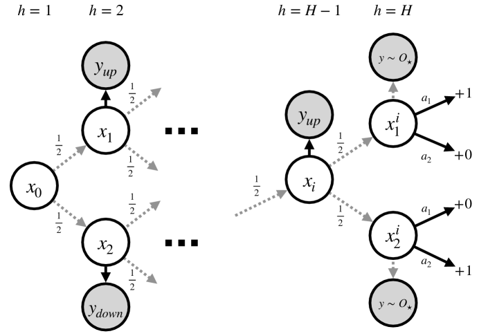
Figure 3: Hard instance of POMDP. The latent state space is a binary tree starting at $x_{0}$ and the learner traverses a layer each time step. The root and and second layer depicted on the left. Observations about which direction it traversed are revealed at each step. In the last and second to last layer, one of many triplets like Figure 2 is encountered (only one depicted in this figure on the right). The policy has no control until the last layer.

In this section, we formally prove the information-theoretic lower bound of Theorem 5.1. We take the standard minimax approach: design a class of problem instances $\mathcal{U}$ such that, for any algorithm that generates a policy $\hat{\pi}$ over $K$ episodes of interaction, there is always a problem instance $u\in\mathcal{U}$ with

$$\mathbb{E}_{u}\left[v(\pi^{\star})-v(\hat{\pi})\right]\geq\epsilon$$

for some $\epsilon$ that we will try to control. The expectation is over the algorithm and data generated under the instance $u$.

While the intuition for the lower bound in the main paper with $X=3$ is useful for understanding how the $Y$ dependence appears in the lower bound, it is not immediate to generalize. Note that it is not sufficient to take the naive approach of simply maintaining $H=1$ and increasing the number of latent states. In such cases, the possible problem instances will either have very low loss separation or be very easy to test and differentiate. This would mean an algorithm could easily either find out how to act optimally or not acting optimally is “close enough.” The issue is that the posterior distribution over $\mathcal{X}$ given an observation would end up being very close to uniform (to avoid being able to simply test to distinguish between instances). However, this allows for a potentially large margin of error for any policy since even the optimal policy will struggle greatly to achieve high rewards regardless.

This issue can be resolved by leveraging the history to reduce the problem to solving many (on the order $X$) $3$-latent state subproblems. Consider the sketch POMDP in Figure 3, which is the full version of the on the one in Figure 2. Figure 3 depicts a binary tree in which the policy randomly traverses the nodes to the leaves of the last layer $H$. The last and second to last layers collectively make up a swath of $3$-latent state problems. The catch is that, as the policy traverses the nodes, the observations reveal its exact state in the tree up to layer $H-1$ by revealing whether it traversed to the upper or lower child at each step with $\{y_{\text{up}},y_{\text{down}}\}$. Thus it can exactly decode its state at layer $H-1$ and find out which of the $3$-latent state problems it is in. At layer $H-1$, it is faced with one of the possible $3$-latent state problems and it must act optimally.

We will design the emission function such that it is difficult to decode whether the learner is in the upper or lower child in the same way as we described for the case when $X=3$. Thus, the learner will have to visit a given $h=H-1$ layer parent at least $\Omega(Y)$ times before learning the optimal policy for that parent. Furthermore, it must learn the optimal policy for at least a constant fraction of the parents (size $\Omega(X)$) to compete with the full optimal policy. Together this yields total interactions on the order of $\Omega(XY)$.

See 5.1

D.1 Construction of instance class

Note that the preconditions ensure that $Y(X+1)\geq 512\log 2$.

The learner starts deterministically at $x_{0}$. Without loss of generality, we assume that $X+1$ is a power of $2$ and $Y$ is even. Otherwise, we can reduce $X+1$ to the nearest power of $2$ and reduce $Y$ to the nearest even number by at most losing a constant factor in the bound. There are a total of $H=\log_{2}(X+1)$ timesteps. Before the $H$th timestep, rewards are all zero and the learner transitions uniformly randomly from the current latent state to either the upper or lower child latent state in the next layer, regardless of the action (see Figure 3). An observation $y_{\text{up}}$ or $y_{\text{down}}$ is revealed indicating whether the learner is currently in the upper or lower child of the parent latent state. Hence, for $h\leq H-1$, the latent state can be exactly decoded given the history of observations. We assume that all states in the final layer $h=H$ then transition to a dummy state such as $x_{0}$ at $H+1$.

We denote the states of the final layer $h=H$ by $\mathcal{X}^{\prime}$. Note that $\mathcal{X}^{\prime}$ consists of $X^{\prime}:={X+1\over 2}$ latent states. States in $\mathcal{X}^{\prime}$ can be grouped into ${X^{\prime}\over 2}$ groups of $2$ where the states in a group share the same parent. Let $x^{1}_{i}$ and $x^{2}_{i}$ be the upper and lower children of the same parent state $x_{i}$, respectively. The reward function is defined as

$$r(x^{1}_{i},a)=\begin{cases}1&a=a_{1}\\ 0&a=a_{2}\end{cases}$$ (172)

$$r(x^{2}_{i},a)=\begin{cases}0&a=a_{1}\\ 1&a=a_{2}\end{cases}$$ (173)

This is duplicated for all the parent-child triplets $(x_{i},x_{i}^{1},x_{i}^{2})$ in the second to last and last layers. The emission function in the final layer is different depending on the parent $x_{i}$ and the child. For a child latent state $x\in\mathcal{X}^{\prime}$, we design $O_{\star}(\cdot|x)$ to be supported on $\mathcal{Y}^{\prime}:=\mathcal{Y}\setminus\{y_{\text{up}},y_{\text{down}}\}$ with cardinality $Y^{\prime}=|\mathcal{Y}^{\prime}|$, which will be specified presently. The instances will vary based on the selection of $O_{\star}$.

D.2 Selection of emission function

We construct the instances by perturbing the probabilities in $O_{\star}$ so that they deviate slightly from uniform. To ensure that probabilities properly sum to $1$, we will split $\mathcal{Y}^{\prime}$ into equal partitions $\mathcal{Y}^{\prime}_{+}$ and $\mathcal{Y}^{\prime}_{-}$ each of size $|Y^{\prime}|\over 2$. We can construct a bijection such that for any $y\in\mathcal{Y}^{\prime}_{-}$ there is a “mirror” $y_{+}$ in $\mathcal{Y}^{\prime}_{+}$. An instance in the class will be specified by some vector $u\in\{-1,1\}^{{X^{\prime}Y^{\prime}\over 4}}$ which determines the observation matrix. We will denote the observation matrix for instance $u$ with $O_{\star,u}$. Fix $\epsilon>0$. We index into the vector $u$ with an observation in $y\in\mathcal{Y}^{\prime}_{+}$ and a parent latent state $x_{i}\in\mathcal{X}$ in the second to last layer. Let $x^{1}_{i}$ and $x^{2}_{i}$ be leaf latent states that share the same parent $x_{i}$. Note that this is valid since the child states (as we construct them) are distinct for each parent. Then for $x^{1}_{i}$, define

$$O_{\star,u}(y|x^{1}_{i})={1+u(y,x_{i})\epsilon\over Y^{\prime}}\quad\forall y\in\mathcal{Y}^{\prime}_{+},$$ (174)

$$O_{\star,u}(y|x^{1}_{i})={1-u(y_{+},x_{i})\epsilon\over Y^{\prime}}\quad\forall y\in\mathcal{Y}^{\prime}_{-},$$ (175)

and for $x_{2}$,

$$O_{\star,u}(y|x^{2}_{i})={1-u(y,x_{i})\epsilon\over Y^{\prime}}\quad\forall y\in\mathcal{Y}^{\prime}_{+},$$ (176)

$$O_{\star,u}(y|x^{2}_{i})={1+u(y_{+},x_{i})\epsilon\over Y^{\prime}}\quad\forall y\in\mathcal{Y}^{\prime}_{-}.$$ (177)

We will also use $P_{u}$ and $\mathbb{E}_{u}$ to denote the measure and expectation, respectively, under instance $u$. We can verify that, conditioned on the the parent $x_{i}$, the distribution over $\mathcal{Y}^{\prime}$ is uniform:

$$P_{u}(y|x_{i}) =P(x_{i}^{1}|x_{i})O_{\star,u}(y|x^{1}_{i})+P(x^{2}_{i}|x_{i})O_{\star,u}(y|x^{2}_{i})$$ (178)

$$={O_{\star,u}(y|x^{1}_{i})+O_{\star,u}(y|x^{2}_{i})\over 2}={1\over Y^{\prime}}.$$ (179)

It is also worth noting that, conditioned on the parent $x_{i}$ (equivalently, on the history $y_{1:H-1}$), the posterior is:

$$P_{u}(x^{1}_{i}|y_{H},x_{i}) ={1+u(y_{H},x_{i})\epsilon\over 2}\quad\forall y\in\mathcal{Y}^{\prime}_{+}$$ (180)

$$P_{u}(x^{1}_{i}|y_{H},x_{i}) ={1-u((y_{H})_{+},x_{i})\epsilon\over 2}\quad\forall y\in\mathcal{Y}^{\prime}_{-}.$$ (181)

Furthermore, by Lemma 4.7 of Massart (2007), there exists $\mathcal{U}\in\{-1,1\}^{X^{\prime}Y^{\prime}/4}$ such that $|\mathcal{U}|\geq\exp(Y^{\prime}X^{\prime}/32)$ and $\|u-u^{\prime}\|_{1}\geq{X^{\prime}Y^{\prime}\over 8}$ for all $u,u^{\prime}\in\mathcal{U}$ such that $u\neq u^{\prime}$.

D.3 Separability condition

We now show in this construction that no history-dependent policy can perform well on all instances in $\mathcal{U}$ simultaneously. Let $\Pi$ be the class of all history-dependent, deterministic policies. Let $u\in\mathcal{U}$ be fixed. It is clear that the optimal policy for instance $u$ chooses action $\hat{a}$ such that $r(\hat{x},\hat{a})=1$ where $\hat{x}=\operatorname*{arg\,max}_{x}P_{u}(x|y_{1:H})\in\mathcal{X}^{\prime}$ maximizes the posterior. We denote this policy by $\pi^{\star}_{u}$.

Consider an arbitrary $\pi$. Recall that, by construction, there is a bijection between $y_{1:H-1}$ and the parent latent states at layer $H-1$. To avoid notational clutter, we will now denote this by $z$ (which we have previously written as $x_{i}$). Thus, we can equivalently write $\pi$ as a function of $z$ and the last observation $y_{H}$. Define

$$v_{u}(\pi|z)=\mathbb{E}_{u}\left[r(x,\pi(y_{H},z))\ |\ z\right]$$ (182)

as the conditional value of $\pi$ given it has reached the parent $z$ in instance $u$. A straightforward calculation shows that

$$v_{u}(\pi^{\star}_{u}|z)-v_{u}(\pi|z)=\epsilon\cdot{N_{z}(\pi,\pi^{\star}_{u})\over Y^{\prime}}$$ (183)

where $N_{z}(\pi,\pi^{\star}_{u}):=\sum_{y\in\mathcal{Y}^{\prime}}\mathbf{1}\left\{\pi^{\star}_{u}(y,z)\neq\pi(y,z)\right\}$ is the number of observations on which $\pi$ and $\pi^{\star}_{u}$ disagree given parent $z$. The sub-optimality gap on the full instance is simply the average over the ${X^{\prime}\over 2}$ parents:

$$v_{u}(\pi^{\star}_{u})-v_{u}(\pi)=\epsilon\sum_{z}{2N_{z}(\pi,\pi^{\star}_{u})\over Y^{\prime}X^{\prime}}={2\epsilon N(\pi,\pi_{u}^{*})\over Y^{\prime}X^{\prime}},$$ (184)

where $N(\pi,\pi_{u}^{*})=\sum_{z}\sum_{y\in\mathcal{Y}^{\prime}}\mathbf{1}\left\{\pi^{\star}_{u}(y,z)\neq\pi(y,z)\right\}$ is the total number of disagreements at layer $H$. Then, for any $u,u^{\prime}\in\mathcal{U}$ such that $u\neq u^{\prime}$,

$$\underbrace{v_{u}(\pi^{\star}_{u})-v_{u}(\pi)}_{\text{error on instance }u}+\underbrace{v_{u^{\prime}}(\pi^{\star}_{u^{\prime}})-v_{u^{\prime}}(\pi)}_{\text{error on instance }u^{\prime}} ={2\epsilon\over Y^{\prime}X^{\prime}}\left(N(\pi,\pi^{\star}_{u})+N(\pi,\pi^{\star}_{u^{\prime}})\right)$$ (185)

$$\geq{2\epsilon N(\pi^{\star}_{u},\pi^{\star}_{u^{\prime}})\over Y^{\prime}X^{\prime}}.$$ (186)

Finally, we recall that $\mathcal{U}$ is such that $\|u-u^{\prime}\|_{1}\geq{X^{\prime}Y^{\prime}\over 8}$, which ensures that $u$ and $u^{\prime}$ differ on at least ${X^{\prime}Y^{\prime}\over 16}$ elements, which implies that $N(\pi^{\star}_{u},\pi^{\star}_{u^{\prime}})\geq{X^{\prime}Y^{\prime}\over 16}$. Thus, we have

$$v_{u}(\pi^{\star}_{u})-v_{u}(\pi)+v_{u^{\prime}}(\pi^{\star}_{u^{\prime}})-v_{u^{\prime}}(\pi) \geq{\epsilon\over 8}$$ (187)

D.4 Fano’s inequality application

Thus far, we have detailed the instance class and shown that no policy can achieve error less than $\epsilon\over 16$ on more than one instance. To complete the proof, we apply Fano’s inequality to show that these instances are essentially indistinguishable.

Let $\hat{\pi}$ be the output of any algorithm $\mathfrak{A}$ that samples from a POMDP instance over $K$ episodes (which a random variable dependent on the instance in which it is run). We have

$$\max_{u\in\mathcal{U}}\mathbb{E}_{u}\left[v_{u}(\pi^{\star}_{u})-v_{u}(\hat{\pi})\right] \geq{\epsilon\over 16}\inf_{\Psi}{1\over|\mathcal{U}|}\sum_{u\in\mathcal{U}}P_{u}\left(\Psi\neq u\right)$$ (188)

where $\Psi$ is a data-dependent test function, the $\inf$ is taken over all measurable tests, $P_{u}$ denotes the measure under instance $u$. By Fano’s inequality,

$$\max_{u\in\mathcal{U}}\mathbb{E}_{u}\left[v_{u}(\pi^{\star}_{u})-v_{u}(\hat{\pi})\right] \geq{\epsilon\over 16}\left(1-{\max_{u\neq u^{\prime}}D_{KL}\left(P_{u}\|P_{u^{\prime}}\right)+\log 2\over\log|\mathcal{U}|}\right)$$ (189)

where $P_{u}$ and $P_{u^{\prime}}$ are measures under instances $u$ and $u^{\prime}$, respectively. Note that these are dependent on the algorithm $\mathfrak{A}$, which determines which actions to take over the $K$ episodes. That is, the probability of taking action $a_{h}^{k}$ in round $k$ at step $h$ is $\mathfrak{A}(a^{k}_{h}|\bar{\tau}^{1:k-1},\bar{\tau}^{k}_{h})$ where we recall that $\bar{\tau}_{h}^{k}=(x_{1:h},y_{1:h},a_{1:h-1})$ is the partial trajectory and $\bar{\tau}^{k}$ is the full trajectory, both containing the latent states. Crucially, note that we allow $\mathfrak{A}$ to be dependent on the latent states. Note that, for HOMDP model, we usually assume that this is further reduced to only dependence on historical observations and actions within the current partial trajectory so that $\bar{\tau}_{h}^{k}$ becomes $\tau_{h}^{k}$ in the conditional part. However, this generality allows us to capture algorithms that also can access the underlying state even during training deployments.

The chain rule of the KL divergence gives us the following decomposition in terms of conditional KL divergences:

$$D_{KL}(P_{u}\|P_{u^{\prime}}) =\sum_{k\in[K]}\mathbb{E}_{\bar{\tau}^{1:k-1}}\left[D_{KL}\left(P_{u}(\bar{\tau}^{k})\|P_{u^{\prime}}(\bar{\tau}^{k})\ |\ \bar{\tau}^{1:k-1}\right)\right].$$

where we abuse notation slightly and let $P_{u}(\bar{\tau}^{k})$ denote the distribution over trajectory $\bar{\tau}^{k}$. Then, the individual terms are also written as

$$\mathbb{E}_{\bar{\tau}^{1:k-1}}\left[D_{KL}\left(P_{u}(\bar{\tau}^{k})\|P_{u^{\prime}}(\bar{\tau}^{k})\ |\ \bar{\tau}^{1:k-1}\right)\right] =\mathbb{E}_{\bar{\tau}^{1:k-1}}\left[\sum_{\bar{\tau}^{k}}P_{u}(\bar{\tau}^{k}\ |\ \bar{\tau}^{1:k-1})\log\frac{P_{u}(\bar{\tau}^{k}\ |\ \bar{\tau}^{1:k-1})}{P_{u^{\prime}}(\bar{\tau}^{k}\ |\ \bar{\tau}^{1:k-1})}\right].$$ (190)

Observe that the conditional probability of a trajectory is

$$P_{u}(\bar{\tau}^{k}\ |\ \bar{\tau}^{1:k-1}) =P_{u}(x_{1}^{k})\prod_{h=1}^{H}O_{\star,u}(y_{h}^{k}|x_{h}^{k})\mathfrak{A}(a_{h}|\bar{\tau}_{h}^{k},\bar{\tau}^{1:k-1})T_{\star,u}(x_{h+1}^{k}|x_{h}^{k},a_{h}^{k})$$ (191)

Between the instances $u$ and $u^{\prime}$, everything is the same (including $\mathfrak{A}$) except for $O_{\star,u}(\cdot|x^{k}_{H})$ and $O_{\star,u^{\prime}}(\cdot|x^{k}_{H})$ in the last layer by construction. Furthermore, we have that $P(x^{k}_{H}|\bar{\tau}^{1:k-1})=P(x^{k}_{H})={1\over X^{\prime}}$ since the policy has no control over the first $H-1$ steps. Therefore, the conditional KL divergence for any $k$ becomes:

$$\mathbb{E}_{\bar{\tau}^{1:k-1}}\left[D_{KL}\left(P_{u}(\bar{\tau}^{k})\|P_{u^{\prime}}(\bar{\tau}^{k})\ |\ \bar{\tau}^{1:k-1}\right)\right] =\sum_{y_{H},x_{H}}P_{u}(x_{H}|\bar{\tau}^{1:k-1}_{H})\log{O_{\star,u}(y_{H}|x_{H})\over O_{\star,u^{\prime}}(y_{H}|x_{H})}$$ (192)

$$={1\over X^{\prime}}\sum_{x_{H}\in\mathcal{X}^{\prime}}\sum_{y_{H}}\log{O_{\star,u}(y_{H}|x_{H})\over O_{\star,u^{\prime}}(y_{H}|x_{H})}$$ (193)

$$={1\over X^{\prime}}\sum_{x\in\mathcal{X}^{\prime}}\sum_{y\in\mathcal{Y}^{\prime}_{-}}O_{\star,u}(y|x)\log{O_{\star,u}(y|x)\over O_{\star,u^{\prime}}(y|x)}+O_{\star,u}(y_{+}|x)\log{O_{\star,u}(y_{+}|x)\over O_{\star,u^{\prime}}(y_{+}|x)}$$ (194)

$$\leq{2\over X^{\prime}Y^{\prime}}\sum_{x\in\mathcal{X}^{\prime},y\in\mathcal{Y}^{\prime}_{-}}(1+\epsilon)\log{1+\epsilon\over 1-\epsilon}+(1-\epsilon)\log{1-\epsilon\over 1+\epsilon}$$ (195)

$$\leq{2\over X^{\prime}Y^{\prime}}\sum_{x\in\mathcal{X}^{\prime},y\in\mathcal{Y}^{\prime}_{-}}8\epsilon^{2}$$ (196)

$$=8\epsilon^{2}$$ (197)

for $\epsilon<{1/2}$. Therefore, for if $K\leq{\log|\mathcal{U}|-2\log 2\over 16\epsilon^{2}}$, we have

$$\max_{u\in\mathcal{U}}\mathbb{E}_{u}\left[v_{u}(\pi^{\star}_{u})-v_{u}(\hat{\pi})\right] \geq{\epsilon\over 16}\left(1-{8K\epsilon^{2}+\log 2\over\log|\mathcal{U}|}\right)$$ (198)

$$\geq{\epsilon\over 32}$$ (199)

From the lower bound on the size of $\mathcal{U}$, we have that

$$K\leq{X^{\prime}Y^{\prime}\over 1024\epsilon^{2}}$$ (200)

implies the above condition because

$$K \leq{X^{\prime}Y^{\prime}\over 1024\epsilon^{2}}$$ (201)

$$\leq{X^{\prime}Y^{\prime}/32-2\log 2\over 16\epsilon^{2}}$$ (202)

$$\leq{\log|\mathcal{U}|-2\log 2\over 16\epsilon^{2}}$$ (203)

as long as $X^{\prime}Y^{\prime}\geq 64\cdot 2\log 2$. Since $Y^{\prime}=Y-2$ and $X^{\prime}={X+1\over 2}$, we have

$$X^{\prime}Y^{\prime}={(X+1)(Y-2)\over 2}\geq{(X+1)Y\over 4}\geq 128\log 2$$

where the second inequality follows from the constraints on $X$ and $Y\geq 6$.

Appendix E Proof of Theorem 6.3

A core component of the analysis is a simulation lemma that bounds the difference in values of a policy on two different POMDPs via the total variation distance of their models.

Lemma E.1 (Simulation Lemma).

Consider a POMDP model with transition matrix $\hat{T}$, emission matrix $\hat{O}$, and reward function $r$. Denote the value function and measure under this POMDP by $\hat{v}$ and $\hat{P}$ respectively. Then, for any history-dependent policy $\pi$,

$$\|\hat{P}_{\pi}-P_{\pi}\|_{1} \leq\mathbb{E}_{\pi}\sum_{h\in[H]}\|O_{\star}(\cdot|x_{h})-\hat{O}(\cdot|x_{h})\|_{1}+\|T_{\star}(\cdot|x_{h},a_{h})-\hat{T}(\cdot|x_{h},a_{h})\|_{1}.$$

Furthermore,

$$|v(\pi)-\hat{v}(\pi)| \leq H\mathbb{E}_{\pi}\sum_{h\in[H]}\|O_{\star}(\cdot|x_{h})-\hat{O}(\cdot|x_{h})\|_{1}+\|T_{\star}(\cdot|x_{h},a_{h})-\hat{T}(\cdot|x_{h},a_{h})\|_{1},$$

where $\mathbb{E}_{\pi}$ denotes the expectation following policy $\pi$ under the true model $\mathcal{M}$.

This observation, although crude sometimes, is useful in this setting because it is possible to estimate the models in HOMDP, in contrast to the POMDP where faithful recovery of $O_{\star}$ and $T_{\star}$ is not always possible.

E.1 High-probability events

Similar to the tabular setting, we define the following events and later show that they each occur with high probability.

$$\mathcal{E}_{\mathcal{T}} =\left\{\forall k\in[K^{\prime}],T\in\mathcal{T},\ \sum_{\ell\in[k],h\in[H]}\|T(\cdot|x_{h}^{\ell},a_{h}^{\ell})-T_{\star}(\cdot|x_{h}^{\ell},a_{h}^{\ell})\|^{2}_{1}\leq 8\log(K^{\prime}|\mathcal{T}|/\delta)+4\sum_{\ell,h}\log{T_{\star}(\tilde{x}^{\ell}_{h}|x^{\ell}_{h},a^{\ell}_{h})\over T(\tilde{x}^{\ell}_{h}|x^{\ell}_{h},a^{\ell}_{h})}\right\}$$

$$\mathcal{E}_{\Theta} =\left\{\forall k\in[K^{\prime}],O\in\Theta,\ \sum_{\ell\in[k],h\in[H]}\|O(\cdot|x_{h}^{\ell})-O_{\star}(\cdot|x_{h}^{\ell})\|^{2}_{1}\leq 8\log(K^{\prime}|\Theta|/\delta)+4\sum_{\ell,h}\log{O_{\star}(y^{\ell}_{h}|x^{\ell}_{h})\over O(y^{\ell}_{h}|x^{\ell}_{h})}\right\}$$

The intersection of the above two is defined as $\mathcal{E}_{\mathcal{T},\Theta}=\mathcal{E}_{\mathcal{T}}\cap\mathcal{E}_{\Theta}$. Finally, let $\mathcal{E}_{\text{Fre}}$ denote the event that,for all $k\in[K^{\prime}]$ and $h\in[H]$, with $\tilde{\pi}_{\ell}=\hat{\pi}_{\ell}\circ_{h}\operatorname*{Unif}(\mathcal{A})$,

$$\sum_{\ell\in[k-1]}\mathbb{E}_{\tilde{\pi}_{\ell}}\left[\|T_{\star}(\cdot|x_{h})-\hat{T}_{k}(\cdot|x_{h},a_{h})\|_{1}^{2}+\|O_{\star}(\cdot|x_{h},a_{h})-\hat{O}_{k}(\cdot|x_{h})\|_{1}^{2}\right]$$ (204)

$$\leq 32\log\left(K^{\prime}H|\mathcal{T}\times\Theta|/\delta\right)+2\sum_{\ell\in[k-1]}\|T_{\star}(\cdot|x_{h}^{\ell},a_{h}^{\ell})-\hat{T}_{k}(\cdot|x_{h}^{\ell},a_{h}^{\ell})\|_{1}^{2}+\|O_{\star}(\cdot|x_{h}^{\ell})-\hat{O}_{k}(\cdot|x_{h}^{\ell})\|_{1}^{2}.$$ (205)

Lemma E.2.

$P(\mathcal{E}_{\mathcal{T}})\geq 1-\delta$.

Proof.

See Appendix E.4. ∎

Lemma E.3.

$P(\mathcal{E}_{\Theta})\geq 1-\delta$.

Proof.

The proof is identical to that of Lemma E.2, except that one replaces $\mathcal{T}$ with $\Theta$, $T_{\star}$ with $O_{\star}$, and the sample pairs $\tilde{x}^{\ell}_{h},x^{\ell}_{h},a^{\ell}_{h}$ with $y^{\ell}_{h},x^{\ell}_{h}$. ∎

Lemma E.4.

$P(\mathcal{E}_{\text{Fre}})\geq 1-\delta$.

Proof.

Fix $T\in\mathcal{T}$ and $O\in\Theta$. For convenience, define

$$\epsilon(x,a)=\|T_{\star}(\cdot|x,a)-T(\cdot|x,a)\|_{1}+\|O_{\star}(\cdot|x)-O(\cdot|x)\|_{1}.$$ (206)

Then, consider the stochastic process given by

$$Z_{\ell}=\epsilon(x_{h}^{\ell},a_{h}^{\ell})$$

It is easy to see that $Z_{\ell}-\mathbb{E}_{\tilde{\pi}_{\ell}}\left[Z_{\ell}\right]$ is a martingale difference sequence with $|Z_{\ell}|\leq 8=:R$ since $x_{h}^{\ell},a_{h}^{\ell}$ are drawn from the exploration policy $\tilde{\pi}_{\ell}$. By Theorem 1 of (Beygelzimer et al., 2011), with probability at least $1-\delta$, for all $k\in[K]$,

$$\sum_{\ell\in[k]}\mathbb{E}_{\tilde{\pi}_{\ell}}\left[Z_{\ell}\right]-Z_{\ell} \leq{1\over 2R}\sum_{\ell\in[k]}\operatorname*{var}_{\tilde{\pi}_{\ell}}\left(Z_{\ell}\right)+2R\log(1/\delta)$$ (207)

where $\operatorname*{var}_{\tilde{\pi}_{\ell}}(Z_{\ell})=\mathbb{E}_{\tilde{\pi}_{\ell}}\left(Z_{\ell}-\mathbb{E}_{\tilde{\pi}_{\ell}}\left[Z_{\ell}\right]\right)^{2}$. Then, note that

$$\operatorname*{var}_{\tilde{\pi}_{\ell}}(Z_{\ell}) \leq\mathbb{E}_{\tilde{\pi}_{\ell}}\left[Z_{\ell}^{2}\right]\leq R\mathbb{E}_{\tilde{\pi}_{\ell}}Z_{\ell}$$

since $0\leq Z_{\ell}\leq R$. Applying this inequality and then rearranging, we have

$$\sum_{\ell\in[k]}\mathbb{E}_{\tilde{\pi}_{\ell}}\left[Z_{\ell}\right] \leq 2\sum_{\ell\in[k]}Z_{\ell}+4R\log(1/\delta)$$

Applying the definition of $Z_{\ell}$ and taking the union bound for all $h\in[H]$, $k\in[K^{\prime}]$, $T\in\mathcal{T}$ and $O\in\Theta$ gives the result with $R=8$. ∎

E.2 Consequences of concentration

Lemma E.5.

Assume that the events $\mathcal{E}_{\mathcal{T},\Theta}$ and $\mathcal{E}_{\text{Fre}}$ hold. For all $k\in[K^{\prime}]$, $T_{\star}\in\mathcal{T}_{k}$ and $O_{\star}\in\Theta_{k}$.

Proof.

Note that from $\mathcal{E}_{\mathcal{T},\Theta}$, it holds that for all $k\in[K^{\prime}]$ and $T\in\mathcal{T}$ and $O\in\Theta$,

$$\sum_{\ell\in[k-1],h}\log T(\tilde{x}^{\ell}_{h}|x^{\ell}_{h},a^{\ell}_{h})-2\log(K^{\prime}|\mathcal{T}|/\delta)\leq\sum_{\ell\in[k-1],h}\log T_{\star}(\tilde{x}^{\ell}_{h}|x^{\ell}_{h},a^{\ell}_{h})$$ (208)

and

$$\sum_{\ell\in[k-1],h}\log O(y^{\ell}_{h}|x^{\ell}_{h})-2\log(K^{\prime}|\Theta|/\delta)\leq\sum_{\ell\in[k-1],h}\log O_{\star}(y^{\ell}_{h}|x^{\ell}_{h})$$ (209)

Given the definitions of $\beta_{\mathcal{T}}$ and $\beta_{\Theta}$, the result is immediate. ∎

Lemma E.6.

Assume that the events $\mathcal{E}_{\mathcal{T},\Theta}$ and $\mathcal{E}_{\text{Fre}}$ hold. Then, for all $k\in[K^{\prime}]$ and $h\in[H]$, with $\tilde{\pi}_{\ell}=\hat{\pi}_{\ell}\circ_{h}\operatorname*{Unif}(\mathcal{A})$,

$$\sum_{\ell\in[k-1]}\mathbb{E}_{\tilde{\pi}_{\ell}}\left[\|T_{\star}(\cdot|x_{h},a_{h})-\hat{T}_{k}(\cdot|x_{h},a_{h})\|_{1}^{2}+\|O_{\star}(\cdot|x_{h})-\hat{O}_{k}(\cdot|x_{h})\|_{1}^{2}\right]$$

$$\leq 32\log(K^{\prime}H|\mathcal{T}\times\Theta|/\delta)+16\left(\beta_{\Theta}+\beta_{\mathcal{T}}\right)$$

Proof.

From $\mathcal{E}_{\text{Fre}}$. Fix $h\in[H]$ and $k\in[K^{\prime}]$. Then,

$$\sum_{\ell}\mathbb{E}_{\tilde{\pi}_{\ell}}\left[\|T_{\star}(\cdot|x_{h},a_{h})-\hat{T}_{k}(\cdot|x_{h},a_{h})\|_{1}^{2}+\|O_{\star}(\cdot|x_{h})-\hat{O}_{k}(\cdot|x_{h})\|_{1}^{2}\right]$$ (210)

$$\leq 32\log(K^{\prime}H|\mathcal{T}\times\Theta|/\delta)+2\sum_{\ell}\|T_{\star}(\cdot|x_{h}^{\ell},a_{h}^{\ell})-\hat{T}_{k}(\cdot|x_{h}^{\ell},a_{h}^{\ell})\|_{1}^{2}+\|O_{\star}(\cdot|x_{h}^{\ell})-\hat{O}_{k}(\cdot|x_{h}^{\ell})\|_{1}^{2}$$ (211)

Then, using $\mathcal{E}_{\mathcal{T},\Theta}$,

$$\sum_{\ell}\|O_{\star}(\cdot|x_{h}^{\ell})-\hat{O}_{k}(\cdot|x_{h}^{\ell})\|_{1}^{2} \leq\sum_{\ell,h}\|O_{\star}(\cdot|x_{h}^{\ell})-\hat{O}_{k}(\cdot|x_{h}^{\ell})\|_{1}^{2}$$ (212)

$$\leq 8\log(K^{\prime}|\Theta|/\delta)+4\sum_{\ell,h}\log{O_{\star}(y^{\ell}_{h}|x^{\ell}_{h})\over\hat{O}_{k}(y^{\ell}_{h}|x^{\ell}_{h})}$$ (213)

$$\leq 16\log(K^{\prime}|\Theta|/\delta)$$ (214)

where the last inequality uses the fact that $\hat{O}_{k}\in\Theta_{k}$ and $\max_{O\in\Theta_{k}}\sum_{\ell,h}\log O(y^{\ell}_{h}|x^{\ell}_{h})\geq\sum_{\ell,h}\log O_{\star}(y^{\ell}_{h}|x^{\ell}_{h})$ since $O_{\star}\in\Theta_{k}$. The same can be done for $\hat{T}_{k}$ and $\mathcal{T}_{k}$. Then the prior display can be bounded as

$$\sum_{\ell}\mathbb{E}_{\tilde{\pi}_{\ell}}\left[\|T_{\star}(\cdot|x_{h},a_{h})-T(\cdot|x_{h},a_{h})\|_{1}^{2}+\|O_{\star}(\cdot|x_{h})-O(\cdot|x_{h})\|_{1}^{2}\right]$$ (215)

$$\leq 32\log(K^{\prime}H|\mathcal{T}\times\Theta|/\delta)+32\left(\log(K^{\prime}|\Theta|/\delta)+\log(K^{\prime}|\mathcal{T}|/\delta)\right)$$ (216)

$$=32\log(K^{\prime}H|\mathcal{T}\times\Theta|/\delta)+16\left(\beta_{\Theta}+\beta_{\mathcal{T}}\right).$$ (217)

∎

E.3 Final steps

The final steps of the proof follow a classic optimism analysis. We let $\hat{v}_{k}$ denote the value function of the POMDP under the model transition function $\hat{T}_{k}$ and emission function $\hat{O}_{k}$ (selected optimistically in the algorithm).

The instantaneous regret for $k\in[K^{\prime}]$ is bounded as

$$v(\pi^{\star})-v(\hat{\pi}_{k}) \leq\hat{v}_{k}(\hat{\pi}_{k})-v(\hat{\pi}_{k})$$ (218)

$$\leq H\sum_{h}\mathbb{E}_{\hat{\pi}_{k}}\|T_{\star}(\cdot|x_{h},a_{h})-\hat{T}_{k}(\cdot|x_{h},a_{h})\|_{1}+\|O_{\star}(\cdot|x_{h})-\hat{O}_{k}(\cdot|x_{h})\|_{1}$$ (219)

where the second line follows from the POMDP Simulation Lemma (Lemma E.1). Next, leveraging the low rank MDP assumption, define the following quantities:

$$\epsilon(T,O,x,a) :=\|T(\cdot|x,a)-T_{\star}(\cdot|x,a)\|_{1}+\|O(\cdot|x)-O_{\star}(\cdot|x)\|_{1}$$ (220)

$$U_{h}(\hat{\pi}_{k}) :=\mathbb{E}_{x_{h-1},a_{h-1}\hat{\pi}_{k}}\left[\phi(x_{h-1},a_{h-1})\right]$$ (221)

$$W_{h}(T,O) =\int_{x_{h}}\psi_{\star}(x_{h})\cdot\sup_{a_{h}}\epsilon(T,O,x_{h},a_{h})\cdot\mathop{}\!\mathrm{d}x_{h}$$ (222)

$$\Sigma_{k,h} :=\lambda I+\sum_{\ell\in[k-1]}U_{h}(\hat{\pi}_{\ell})U_{h}(\hat{\pi}_{\ell})^{\top}$$ (223)

for some $\lambda>0$ to be determined later. For $h-1=0$, we can take $U_{h}$ to be a fixed indicator and $W_{h}$ to also be an indicator with a non-zero value of $\mathbb{E}_{x_{1}\sim\rho}\sup_{a}\epsilon(T,O,x_{1},a)$. The algorithm does not need to use the vector functions $U_{h}$ or $W_{h}$ or the covariance matrix $\Sigma_{k,h}$. Only the analysis uses them. Then, for a fixed $h\in[H]$, let $\tilde{\pi}_{\ell}=\hat{\pi}_{\ell}\circ_{h}\operatorname*{Unif}(\mathcal{A})$ be the exploration policy used in round $\ell$ for timestep $h$. Then, letting $\tau_{h}$ denote the concatenation of $(\tau_{h-1},a_{h-1},y_{h})$ as usual,

$$\mathbb{E}_{\hat{\pi}_{k}}\|T_{\star}(\cdot|x_{h},a_{h})-\hat{T}_{k}(\cdot|x_{h},a_{h})\|_{1}+\|O_{\star}(\cdot|x_{h})-\hat{O}_{k}(\cdot|x_{h})\|_{1}$$ (224)

$$=\mathbb{E}_{x_{h-1},a_{h-1},\tau_{h-1}\sim\hat{\pi}_{k}}\left<\phi_{\star}(x_{h-1},a_{h-1}),\int_{y_{h},x_{h},a_{h}}\psi_{\star}(x_{h})O_{\star}(y_{h}|x_{h})\hat{\pi}_{k}(a_{h}|\tau_{h})\epsilon(\hat{T}_{k},\hat{O}_{k},x_{h},a_{h})\cdot\mathop{}\!\mathrm{d}(y_{h},x_{h},a_{h})\right>$$ (225)

$$\leq\mathbb{E}_{x_{h-1},a_{h-1}\sim\hat{\pi}_{k}}\left<\phi_{\star}(x_{h-1},a_{h-1}),\int_{y_{h},x_{h}}\psi_{\star}(x_{h})O_{\star}(y_{h}|x_{h})\sup_{a_{h}}\epsilon(\hat{T}_{k},\hat{O}_{k},x_{h},a_{h})\cdot\mathop{}\!\mathrm{d}(y_{h},x_{h})\right>$$ (226)

$$\leq\|U_{h}(\hat{\pi}_{k})\|_{\Sigma_{k,h}^{-1}}\cdot\left\lVert\int_{x_{h}}\psi_{\star}(x_{h})\sup_{a_{h}}\epsilon(\hat{T}_{k},\hat{O}_{k},x_{h},a_{h})\cdot\mathop{}\!\mathrm{d}x_{h}\right\rVert_{\Sigma_{k,h}}$$ (227)

$$=\|U_{h}(\hat{\pi}_{k})\|_{\Sigma_{k,h}^{-1}}\cdot\|W_{h}(\hat{T}_{k},\hat{O}_{k})\|_{\Sigma_{k,h}}.$$ (228)

The first line uses the definition of the low-rank latent transition to decompose the expectation over elements at step $h$. The first inequality replaces the distribution over $a_{h}$ with a $\sup$, which is valid because $\phi_{\star}(x_{h-1},a_{h-1})^{\top}\psi_{\star}(x_{h})\geq 0$ is a probability. The second inequality applies the Cauchy-Schwarz inequality with the definition of $U_{h}$ and the last line uses the definition of $W_{h}$. For the right-hand factor,

$$\lVert W_{h}(\hat{T}_{k},\hat{O}_{k})\rVert_{\Sigma_{k,h}}^{2} =\lambda\|W_{h}(\hat{T}_{k},\hat{O}_{k})\|_{2}^{2}+\sum_{\ell\in[k-1]}\left<U_{h}(\hat{\pi}_{\ell}),W_{h}(\hat{T}_{k},\hat{O}_{k})\right>^{2}$$ (229)

Using the normalization condition on $\psi_{\star}$, we have

$$\lambda\|W_{h}(\hat{T}_{k},\hat{O}_{k})\|_{2}^{2} \leq 8\lambda d$$ (230)

Also,

$$\sum_{\ell\in[k-1]}\left<U_{h}(\hat{\pi}_{\ell}),W_{h}(\hat{T}_{k},\hat{O}_{k})\right>^{2}$$ (231)

$$=\sum_{\ell\in[k-1]}\left(\mathbb{E}_{x_{h}\sim\hat{\pi}_{\ell}}\sup_{a_{h}}\epsilon(\hat{T}_{k},\hat{O}_{k},x_{h},a_{h})\right)^{2}$$ (232)

$$\leq 2\sum_{\ell\in[k-1]}\mathbb{E}_{x_{h}\sim\hat{\pi}_{\ell}}\sup_{a_{h}}\left[\|T_{\star}(\cdot|x_{h},a_{h})-\hat{T}_{k}(\cdot|x_{h},a_{h})\|_{1}^{2}+\|O_{\star}(\cdot|x_{h})-\hat{O}_{k}(\cdot|x_{h})\|_{1}^{2}\right]$$ (233)

$$\leq 2A\sum_{\ell\in[k-1]}\mathbb{E}_{x_{h},a_{h}\sim\tilde{\pi}_{\ell}}\left[\|T_{\star}(\cdot|x_{h},a_{h})-\hat{T}_{k}(\cdot|x_{h},a_{h})\|_{1}^{2}+\|O_{\star}(\cdot|x_{h})-\hat{O}_{k}(\cdot|x_{h})\|_{1}^{2}\right].$$ (234)

The first inequality above applies Jensen’s inequality and the fact that $(a+b)^{2}\leq 2(a^{2}+b^{2})$. The second inequality upper bounds the $\sup_{a_{h}}$ with a sum to convert the expression to a uniform distribution over $a_{h}$, which is exactly the distribution under the exploration policy $\tilde{\pi}_{\ell}$. Therefore, leveraging Lemma E.6 under $\mathcal{E}_{\Theta}$, $\mathcal{E}_{\mathcal{T}}$, and $\mathcal{E}_{\text{Fre}}$,

$$\lVert W_{h}(\hat{T}_{k},\hat{O}_{k})\rVert_{\Sigma_{k,h}}^{2} \leq 8\lambda d+64A\left(\log\left(K^{\prime}H|\mathcal{T}\times\Theta|/\delta\right)+\beta_{\mathcal{T}}+\beta_{\Theta}\right)$$ (235)

Then,

$$\mathbb{E}_{\hat{\pi}_{k}}\|T_{\star}(\cdot|x_{h},a_{h})-\hat{T}_{k}(\cdot|x_{h},a_{h})\|_{1}+\|O_{\star}(\cdot|x_{h})-\hat{O}_{k}(\cdot|x_{h})\|_{1}$$ (236)

$$\leq\min\left\{4,{\sqrt{64A}}\lVert U_{h}(\hat{\pi}_{k})\rVert_{\Sigma^{-1}_{k,h}}\sqrt{\lambda d+\beta_{\mathcal{T}}+\beta_{\Theta}+\log(K^{\prime}H|\mathcal{T}\times\Theta|/\delta)}\right\}$$ (237)

Let $\beta_{\lambda}:={\lambda d+\beta_{\mathcal{T}}+\beta_{\Theta}+\log(K^{\prime}H|\mathcal{T}\times\Theta|/\delta)}$ for shorthand. Then, the total sub-optimality of the proposed policies $\hat{\pi}_{1},\ldots,\hat{\pi}_{K}$ is bounded as

$$\sum_{k\in[K^{\prime}]}v(\pi^{\star})-v(\hat{\pi}_{k}) \leq H\sum_{k,h}\left(4\wedge\lVert U_{h}(\hat{\pi}_{k})\rVert_{\Sigma^{-1}_{k,h}}\cdot\sqrt{64\beta_{\lambda}A}\right)$$ (238)

$$\leq{H}\sum_{h}\sqrt{64\beta_{\lambda}AK\sum_{k}\left(1\wedge\lVert U_{h}(\hat{\pi}_{k})\rVert^{2}_{\Sigma^{-1}_{k,h}}\right)}$$ (239)

$$\leq{H^{2}}\sqrt{64\beta_{1/d}AKd\log(1+K^{\prime})}$$ (240)

where the last inequality applies the elliptical potential lemma (Lemma F.8) with the setting $\lambda=\nicefrac{{1}}{{d}}$.

E.4 Proof of Lemma E.2

Proof.

The proof follows a similar approach as Agarwal et al. (2020). Fix $k\in[K^{\prime}]$. In contrast to the the rest of the paper, in this proof only we use $\bar{\tau}^{\ell}$ to denote the data collected, since these differ from the histories in the usual sense as a result of the exploration happening over $H$ rounds per epoch. In particular, we define $\bar{\tau}^{\ell}=\left\{x_{h}^{\ell},a_{h}^{\ell},y_{h}^{\ell},\tilde{x}_{h}^{\ell}\right\}_{h=\in[H]}$ where we recall in the algorithm that $\tilde{x}_{h}^{\ell}$ is the next-state sampled by the exploration policy for step $h$.

Given the full trajectories $\bar{\tau}^{1},\ldots,\bar{\tau}^{k}$, define the tangent dataset sampled independently as $\hat{x}^{\ell}_{h+1}\sim T_{\star}(\cdot|x^{\ell}_{h},a^{\ell}_{h})$ for $\ell\in[k]$, which has a distribution completely determined by the history. Let $l:\mathcal{X}^{2}\times\mathcal{A}\to\mathbb{R}$ be an arbitrary measurable loss function. Define $L=\sum_{\ell,h}l(x^{\ell}_{h},a^{\ell}_{h},\tilde{x}^{\ell}_{h})$ and $\hat{L}=\sum_{\ell,h}l(x^{\ell}_{h},a^{\ell}_{h},\hat{x}^{\ell}_{h})$. For convenience, let us define $\bar{\boldsymbol{\tau}}^{\ell}_{h}$ to be the concatenated sequence $(\bar{\tau}^{1:\ell-1},\bar{\tau}^{\ell}_{h},a_{h}^{\ell})$.

Consider the function:

$$\exp\left(L-\log\mathbb{E}\left[\exp(\hat{L})\ |\ \bar{\boldsymbol{\tau}}^{k}_{H}\right]\right) ={\exp(L)\over\mathbb{E}\left[\exp(\hat{L})\ |\ \bar{\boldsymbol{\tau}}^{k}_{H}\right]}$$

$$={\exp(L)\over\prod_{\ell,h}\mathbb{E}\left[\exp l(x^{\ell}_{h},a^{\ell}_{h},\hat{x}^{\ell}_{h})\ |\ \bar{\boldsymbol{\tau}}^{\ell}_{h}\right]}$$

where the second equality follows from the fact that the tangent observations are independent given the history of latent states. Then,

$$\mathbb{E}\left[\exp\left(L-\log\mathbb{E}\left[\exp(\hat{L})\ |\ \bar{\boldsymbol{\tau}}^{k}_{h}\right]\right)\right] =\mathbb{E}\left[{\exp(L)\over\prod_{\ell,h}\mathbb{E}\left[\exp l(x^{\ell}_{h},a^{\ell}_{h},\hat{x}^{\ell}_{h})\ |\ \bar{\boldsymbol{\tau}}^{\ell}_{h}\right]}\right]$$ (241)

$$=\mathbb{E}\left[{\prod_{\ell,h}\exp l(x^{\ell}_{h},a^{\ell}_{h},\tilde{x}^{\ell}_{h})\over\prod_{\ell,h}\mathbb{E}\left[\exp l(x^{\ell}_{h},a^{\ell}_{h},\hat{x}^{\ell}_{h})\ |\ \bar{\boldsymbol{\tau}}^{\ell}_{h}\right]}\right]$$ (242)

$$=\mathbb{E}\left[{\prod_{\ell\in[k],h\in[H-1]}\exp\left(l(x^{\ell}_{h},a^{\ell}_{h},\tilde{x}^{\ell}_{h})\right)\over\prod_{\ell\in[k],h\in[H-1]}\mathbb{E}\left[\exp l(x^{\ell}_{h},a^{\ell}_{h},\hat{x}^{\ell}_{h+1})\ |\ \bar{\boldsymbol{\tau}}^{\ell}_{h}\right]}\cdot{\mathbb{E}\left[\exp\left(l(x^{k}_{H},a^{k}_{H},\tilde{x}^{k}_{H})\right)\ |\ \bar{\boldsymbol{\tau}}^{k}_{H}\right]\over\mathbb{E}\left[\exp\left(l(x^{k}_{H},a^{k}_{H},\hat{x}^{k}_{H})\right)\ |\ \bar{\boldsymbol{\tau}}^{k}_{H}\right]}\right]$$ (243)

$$=\mathbb{E}\left[{\prod_{\ell\in[k],h\in[H-1]}\exp\left(l(x^{\ell}_{h},a^{\ell}_{h},\tilde{x}^{\ell}_{h+1})\right)\over\prod_{\ell\in[k],h\in[H-1]}\mathbb{E}\left[\exp l(x^{\ell}_{h},a^{\ell}_{h},\hat{x}^{\ell}_{h+1})\ |\ \bar{\boldsymbol{\tau}}^{\ell}_{h}\right]}\right]$$ (244)

$$=\ldots$$ (245)

$$=1$$ (246)

where the cancellation is repeated for all $\ell\in[k]$ and $h\in[H]$. Applying Markov’s inequality ensures that

$$P\left(L-\log\mathbb{E}\left[\exp(\hat{L})\ |\ \bar{\boldsymbol{\tau}}^{k}_{H}\right]\geq z\right) \leq{\mathbb{E}\left[\exp\left(L-\log\mathbb{E}\left[\exp(\hat{L})\ |\ \bar{\boldsymbol{\tau}}^{k}_{H}\right]\right)\right]\over e^{z}}.$$ (247)

Taking $z=\log(1/\delta)$ guarantees that

$$L-\log\mathbb{E}\left[\exp(\hat{L})\ |\ \bar{\boldsymbol{\tau}}^{k}_{H}\right]\leq\log(1/\delta)$$ (248)

with probability at least $1-\delta$.

We will define the loss function as $\ell(x,a,x^{\prime})=\log\sqrt{T(x^{\prime}|x,a)\over T_{\star}(x^{\prime}|x,a)}$ for some $T\in\mathcal{T}$. One can then relate the above loss function to the total variation distance:

$$\sum_{\ell\in[k],h\in[H]}\|T_{\star}(\cdot|x^{\ell}_{h},a^{\ell}_{h})-T(\cdot|x^{\ell}_{h},a^{\ell}_{h})\|^{2}_{1} =\sum_{\ell,h}\left(\int_{x^{\prime}\in\mathcal{X}}|T_{\star}(x^{\prime}|x^{\ell}_{h},a_{h}^{\ell})-T(x^{\prime}|x^{\ell}_{h},a_{h}^{\ell})|\mathop{}\!\mathrm{d}x^{\prime}\right)^{2}$$ (249)

$$\leq 4\sum_{\ell,h}\int_{x^{\prime}}\left(\sqrt{T_{\star}(x^{\prime}|x^{\ell}_{h},a^{\ell}_{h})}-\sqrt{T(x^{\prime}|x^{\ell}_{h},a^{\ell}_{h})}\right)^{2}\mathop{}\!\mathrm{d}x^{\prime}$$ (250)

$$=8\sum_{\ell,h}\mathbb{E}_{x^{\prime}\sim T_{\star}(\cdot|x^{\ell}_{h},a^{\ell}_{h})}\left[1-\sqrt{T(x^{\prime}|x^{\ell}_{h},a^{\ell}_{h})/T_{\star}(x^{\prime}|x^{\ell}_{h},a^{\ell}_{h})}\right]$$ (251)

$$\leq-8\sum_{\ell,h}\log\mathbb{E}_{x^{\prime}\sim T_{\star}(\cdot|x^{\ell}_{h},a^{\ell}_{h})}\sqrt{T(x^{\prime}|x^{\ell}_{h},a^{\ell}_{h})\over T_{\star}(x^{\prime}|x^{\ell}_{h},a^{\ell}_{h})}$$ (252)

where the first inequality is from Cauchy-Schwarz and the second uses the fact that $\log(1+a)\leq a$ for $a>-1$. Observe that we have

$$-\log\mathbb{E}\left[\exp(\hat{L})\ |\ \bar{\boldsymbol{\tau}}^{k}_{H}\right] =-\log\mathbb{E}\left[\prod_{\ell,h}\exp\left(\log\left(\sqrt{T(\hat{x}^{\ell}_{h+1}|x^{\ell}_{h},a^{\ell}_{h})\over T_{\star}(\hat{x}^{\ell}_{h+1}|x^{\ell}_{h},a^{\ell}_{h})}\right)\right)\ |\ \bar{\boldsymbol{\tau}}^{k}_{H}\right]$$ (253)

$$=-\sum_{\ell,h}\log\left(\mathbb{E}_{x^{\prime}\sim T_{\star}(\cdot|x^{\ell}_{h},a^{\ell}_{h})}\sqrt{T(x^{\prime}|x^{\ell}_{h},a^{\ell}_{h})\over T_{\star}(x^{\prime}|x^{\ell}_{h},a^{\ell}_{h})}\right)$$ (254)

Combining this with the concentration inequality from earlier, we conclude that

$$\sum_{\ell,h}\|T_{\star}(\cdot|x^{\ell}_{h},a^{\ell}_{h})-T(\cdot|x^{\ell}_{h},a^{\ell}_{h})\|^{2}_{1} \leq-8\log\mathbb{E}\left[\exp(\hat{L})\ |\ \mathbf{x}^{k}_{H}\right]$$ (255)

$$\leq-8\left(L-\log(1/\delta)\right)$$ (256)

$$=-8\left({1\over 2}\sum_{\ell,h}\log\left({T(x^{\ell}_{h+1}|x^{\ell}_{h},a^{\ell}_{h})\over T_{\star}(x^{\ell}_{h+1}|x^{\ell}_{h},a^{\ell}_{h})}\right)-\log(1/\delta)\right)$$ (257)

with probability at least $1-\delta$ for a fixed $T$. Taking the union bound over all $T\in\mathcal{T}$ and all $k\in[K^{\prime}]$,

$$\sum_{\ell\in[k],h\in[H]}\|T_{\star}(\cdot|x^{\ell}_{h},a^{\ell}_{h})-T(\cdot|x^{\ell}_{h},a^{\ell}_{h})\|_{1}^{2} \leq 8\log(K^{\prime}|\mathcal{T}|/\delta)+4\sum_{\ell,h}\log\frac{T_{\star}(x^{\ell}_{h+1}|x^{\ell}_{h},a^{\ell}_{h})}{T(x^{\ell}_{h+1},x^{\ell}_{h},a^{\ell}_{h})}$$ (258)

with probability at least $1-\delta$. ∎

Appendix F Auxiliary Lemmas

Here state and prove a number of helpful auxiliary results for the main theorems.

F.1 Simulation lemma

See E.1

Proof.

Note that

$$|v(\pi)-\hat{v}(\pi)| \leq H\|P_{\pi}-\hat{P}_{\pi}\|_{1}$$

where $P_{\pi}$ denotes the measure over trajectories $\bar{\tau}=(x_{1},y_{1},a_{1},\ldots,x_{H},y_{H},a_{H})$ including the latent states under the true model with $T$ and $O$ and policy $\pi$. Similarly $\hat{P}_{\pi}$ denotes the same measure but under the model with $\hat{T}$ and $\hat{O}$. With notation slightly abused, we also use $P_{\pi}(\bar{\tau})$ to denote the density. This density decomposes as

$$P_{\pi}(\bar{\tau})=\rho(x_{1})\left(\prod_{h\in[H-1]}T_{\star}(x_{h+1}|x_{h},a_{h})O_{\star}(y_{h}|x_{h})\pi(a_{h}|\tau_{h})\right)O_{\star}(y_{H}|x_{H})\pi(a_{H}|\tau_{H}),$$

where we recall that $\tau_{h}=(y_{1:h},a_{1:h-1})$ is the partial history. $\hat{P}_{\pi}$ is analogously defined. Consider for now a fixed $\bar{\tau}$. To bound the total variation distance, we are interested in bounding the differences between $P_{\pi}(\bar{\tau})$ and $\hat{P}_{\pi}(\bar{\tau})$. For shorthand, we will define the following quantities:

$$B_{h} =\rho(x_{1})O_{\star}(y_{1}|x_{1})\prod_{t\in[h-1]}T_{\star}(x_{t+1}|x_{t},a_{t})O_{\star}(y_{t+1}|x_{t+1}),$$

$$\bar{\pi}_{h} =\prod_{t\in[h]}\pi(a_{t}|\tau_{t}).$$

Note that we have the following recursion:

$$B_{h}=O_{\star}(y_{h}|x_{h})T_{\star}(x_{h}|x_{h-1},a_{h-1})B_{h-1}$$ (259)

where $B_{1}=\rho(x_{1})O_{\star}(y_{1}|x_{1})$. We also define $\hat{B}_{h}$ analogously with $\hat{O}$ and $\hat{T}$. To prove Lemma E.1, we will recursively apply the following bound.

Lemma F.1.

The following inequality holds:

$$\int_{x_{h},y_{h},a_{h}}\bar{\pi}_{h}|B_{h}-\hat{B}_{h}|\cdot\mathop{}\!\mathrm{d}(x_{h},y_{h},a_{h}) \leq\bar{\pi}_{h-1}\int_{x_{h}}T_{\star}(x_{h}|x_{h-1},a_{h-1})B_{h-1}\cdot\|O_{\star}(\cdot|x_{h})-\hat{O}(\cdot|x_{h})\|_{1}\cdot\mathop{}\!\mathrm{d}x_{h}$$ (260)

$$\quad+\bar{\pi}_{h-1}B_{h-1}\cdot\|T_{\star}(\cdot|x_{h-1},a_{h-1})-\hat{T}(\cdot|x_{h-1},a_{h-1})\|_{1}$$ (261)

$$\quad+\bar{\pi}_{h-1}|B_{h-1}-\hat{B}_{h-1}|$$ (262)

Summing over all possible latent-augmented trajectories, this implies that we have

$$\int_{\bar{\tau}}|P_{\pi}(\bar{\tau})-P_{\pi}(\bar{\tau})|\cdot\mathop{}\!\mathrm{d}\bar{\tau} =\int_{\bar{\tau}}\bar{\pi}_{H}|B_{H}-\hat{B}_{H}|\cdot\mathop{}\!\mathrm{d}\bar{\tau}$$ (263)

$$\leq\sum_{h}\int_{x_{h}}P_{\pi}(x_{h})\cdot\|O_{\star}(\cdot|x_{h})-\hat{O}(\cdot|x_{h})\|_{1}\cdot\mathop{}\!\mathrm{d}x_{h}$$ (264)

$$\quad+\sum_{h\in[H-1]}\int_{x_{h},a_{h}}P_{\pi}(x_{h},a_{h})\cdot\|T_{\star}(\cdot|x_{h},a_{h})-\hat{T}(\cdot|x_{h},a_{h})\|_{1}$$ (265)

$$=\mathbb{E}_{\pi}\sum_{h}\|O_{\star}(\cdot|x_{h})-\hat{O}(\cdot|x_{h})\|_{1}+\mathbb{E}_{\pi}\sum_{h\in[H-1]}\|T_{\star}(\cdot|x_{h},a_{h})-\hat{T}(\cdot|x_{h},a_{h})\|_{1}.$$ (266)

∎

F.1.1 Proof of Lemma F.1

See F.1

Proof.

We first average out $a_{h}$ and then apply the triangle inequality to bound the quantity in terms of the difference in emission matrices $\|O(\cdot|x_{h})-\hat{O}(\cdot|x_{h})\|_{1}$:

$$\int_{x_{h},y_{h},a_{h}}\bar{\pi}_{h}|B_{h}-\hat{B}_{h}|\cdot\mathop{}\!\mathrm{d}(x_{h},y_{h},a_{h})$$ (267)

$$=\bar{\pi}_{h-1}\int_{x_{h},y_{h}}|B_{h}-\hat{B}_{h}|\cdot\mathop{}\!\mathrm{d}(x_{h},y_{h})$$ (268)

$$=\bar{\pi}_{h-1}\int_{x_{h},y_{h}}|T_{\star}(x_{h}|x_{h-1},a_{h-1})O_{\star}(y_{h}|x_{h})B_{h-1}-\hat{T}(x_{h}|x_{h-1},a_{h-1})\hat{O}(y_{h}|x_{h})\hat{B}_{h-1}|\cdot\mathop{}\!\mathrm{d}(x_{h},y_{h})$$ (269)

$$\leq\bar{\pi}_{h-1}\int_{x_{h},y_{h}}T_{\star}(x_{h}|x_{h-1},a_{h-1})B_{h-1}\cdot|O_{\star}(y_{h}|x_{h})-\hat{O}(y_{h}|x_{h})|\cdot\mathop{}\!\mathrm{d}(x_{h},y_{h})$$ (270)

$$\quad+\bar{\pi}_{h-1}\int_{x_{h},y_{h}}\hat{O}(y_{h}|x_{h})|T_{\star}(x_{h}|x_{h-1},a_{h-1})B_{h-1}-\hat{T}(x_{h}|x_{h-1},a_{h-1})\hat{B}_{h-1}|\cdot\mathop{}\!\mathrm{d}(x_{h},y_{h})$$ (271)

$$=\underbrace{\bar{\pi}_{h-1}\int_{x_{h}}T_{\star}(x_{h}|x_{h-1},a_{h-1})B_{h-1}\cdot\|O_{\star}(\cdot|x_{h})-\hat{O}(\cdot|x_{h})\|_{1}\cdot\mathop{}\!\mathrm{d}(x_{h})}_{\textbf{(I)}}$$ (272)

$$\quad+\bar{\pi}_{h-1}\int_{x_{h}}|T_{\star}(x_{h}|x_{h-1},a_{h-1})B_{h-1}-\hat{T}(x_{h}|x_{h-1},a_{h-1})\hat{B}_{h-1}|\cdot\mathop{}\!\mathrm{d}(x_{h}).$$ (273)

Now, we can also apply the triangle inequality to the last term on the right side to bound the quantity in terms of the difference in transition matrices:

$$\int_{x_{h},y_{h},a_{h}}\bar{\pi}_{h}|B_{h}-\hat{B}_{h}|\cdot\mathop{}\!\mathrm{d}(x_{h},y_{h},a_{h}) \leq\textbf{(I)}+\bar{\pi}_{h-1}B_{h-1}\int_{x_{h}}|T_{\star}(x_{h}|x_{h-1},a_{h-1})-\hat{T}(x_{h}|x_{h-1},a_{h-1})|\cdot\mathop{}\!\mathrm{d}(x_{h})$$ (274)

$$\quad+\bar{\pi}_{h-1}\int_{x_{h}}\hat{T}(x_{h}|x_{h-1},a_{h-1})|B_{h-1}-\hat{B}_{h-1}|\cdot\mathop{}\!\mathrm{d}(x_{h})$$ (275)

$$\leq\textbf{(I)}+\bar{\pi}_{h-1}B_{h-1}\cdot\|T(\cdot|x_{h-1},a_{h-1})-\hat{T}(\cdot|x_{h-1},a_{h-1})\|_{1}$$ (276)

$$\quad+\bar{\pi}_{h-1}|B_{h-1}-\hat{B}_{h-1}|.$$ (277)

This concludes the proof. ∎

F.2 Concentration inequalities

Lemma F.2 (Hoeffding’s inequality).

Let $Z_{1},\ldots,Z_{n}$ be a sequence of independent random variables with $Z_{i}\in[a,b]$ for all $i$ for $-\infty<a\leq b<\infty$. Then

$$P\left({1\over n}\sum_{i}Z_{i}-\mathbb{E}[Z_{i}]\geq(b-a)\sqrt{\log(1/\delta)\over n}\right)\leq\delta.$$

Lemma F.3 (Bernstein’s inequality).

Let $Z_{1},\ldots,Z_{n}$ be a sequence of independent random variables with $Z_{i}\in[0,1]$ and variance $\operatorname*{var}(Z_{i})=\sigma^{2}$ and mean $\mathbb{E}[Z_{i}]=\mu$ for all $i$. Then, with probability at least $1-\delta$,

$${1\over n}\sum_{i}Z_{i}-\mathbb{E}[Z_{i}]\leq{\log(1/\delta)\over 3n}+\sqrt{2\sigma^{2}\log(1/\delta)\over n}.$$

Furthermore, this implies that, for all $c\geq 1$,

$${1\over n}\sum_{i}Z_{i}-\mu \leq{\log(1/\delta)\over 3n}+\sqrt{2\mu\log(1/\delta)\over n}$$

$$\leq{\mu\over 2c}+{2c\log(1/\delta)\over n}.$$

Proof.

The first statement is simply the original statement of Bernstein’s inequality. The second uses the fact that $\sigma^{2}\leq\mu$ for variables in $[0,1]$. The last one uses the AM-GM inequality. ∎

Lemma F.4 (Azuma-Hoeffding).

Let $Z_{1},\ldots,Z_{n}$ be a martingale difference sequence with $|Z_{i}|\leq G$ for all $i$. Then, with probability at least $1-\delta$,

$$\sum_{i}Z_{i}\leq 4G\sqrt{n\log(1/\delta)}.$$ (278)

F.3 Pigeonhole lemmas

Lemma F.5 (Pigeonhole Principle).

The following inequalities hold:

$$\sum_{k\in[K],h\in[H]}\sqrt{1\over\max\{1,n_{k}(x_{h}^{k})\}}\leq HX+3\sqrt{HXK}$$ (279)

and

$$\sum_{k\in[K],h\in[H]}\sqrt{1\over\max\{1,n_{k}(x_{h}^{k},a_{h}^{k})\}}\leq HXA+3\sqrt{HXAK}.$$ (280)

Proof.

We prove only the first as the second is equivalent up to summations over the actions. Note that

$$\sum_{k\in[K],h\in[H]}\sqrt{1\over\max\{1,n_{k}(x_{h}^{k})\}} =\sum_{x}\sum_{k=1}^{K}{m_{k}(x)\over\sqrt{\max\{1,n_{k}(x)\}}}$$ (281)

$$\leq XH+\sum_{x}\sum_{k=1}^{K}{m_{k}(x)\over\sqrt{\max\{H,n_{k}(x)\}}},$$ (282)

where $m_{k}(x)=\sum_{h\in[H]}\mathbf{1}\{x^{k}_{h}=x\}$ counts the number of occurrences of $x$ in a single round $k$. The inequality uses the fact that, for any $x$, the summand can contribute at most $H$ to the sum (because $m_{k}(x)$ is bounded by $H$) before $n_{k}(x)$ has value at least $H$. Now we use Lemma F.6 (which is adapted from Lemma 19 of (Auer et al., 2008)) to bound the second term:

$$\sum_{k\in[K],h\in[H]}\sqrt{1\over\max\{H,n_{k}(x_{h}^{k})\}} \leq XH+3\sum_{x}\sqrt{n_{K}(x)}$$ (283)

$$\leq XH+3\sqrt{HXK},$$ (284)

where the last line follows from the Cauchy-Schwarz inequality along with the fact that $\sum_{x}n_{K}(x)=KH$.

∎

Lemma F.6 (Adapted from Auer et al. (2008)).

Let $z_{1},\ldots,z_{n}\in[0,H]$ be an arbitrary sequence and let $Z_{k}=\max\{H,\sum_{k=1}^{k}z_{k}\}$. Then,

$$\sum_{k\in[n]}{z_{k}\over\sqrt{Z_{k-1}}}\leq 3\sqrt{Z_{n}}.$$ (285)

Proof.

Consider the case where $n=1$. Then, $Z_{0}=H$. Furthermore,

$$\sum_{k\in[n]}{z_{k}\over\sqrt{Z_{k}-1}} ={z_{1}\over\sqrt{H}}\leq\sqrt{H}\leq 3\sqrt{Z_{1}}$$ (286)

By induction on the base case, we have

$$\sum_{k\in[n]}{z_{k}\over\sqrt{Z_{k-1}}} =3\sqrt{Z_{n-1}}+{z_{n}\over\sqrt{Z_{n-1}}}$$ (287)

$$\left(3\sqrt{Z_{n-1}}+{z_{n}\over\sqrt{Z_{n-1}}}\right)^{2} =9Z_{n-1}+6z_{n}+{z_{n}^{2}\over Z_{n-1}}$$ (288)

$$\leq 9Z_{n-1}+7z_{n}$$ (289)

$$\leq 9Z_{n}$$ (290)

Therefore, by taking the square root,

$$\sum_{k\in[n]}{z_{k}\over\sqrt{Z_{k-1}}} \leq 3\sqrt{Z_{n}}$$ (291)

∎

Lemma F.7.

The following inequality holds:

$$\sum_{k\in[K],h\in[H]}{1\over\max\left\{1,n_{k}(x_{h}^{k},a_{h}^{k})\right\}}\leq HXA(1+\log K).$$ (292)

Proof.

First note that since $n_{k}(x,a)$ is updated each episode, we immediately have

$$\sum_{k\in[K],h\in[H]}{1\over\max\left\{1,n_{k}(x_{h}^{k})\right\}} \leq HXA\sum_{i=1}^{\lceil K/XA\rceil}{1\over i}$$ (293)

$$\leq HXA\sum_{i=1}^{K}{1\over i}$$ (294)

since we assume that $X,A\geq 1$. Then,

$$\sum_{i\in[K]}\frac{1}{i}\leq 1+\int_{1}^{K}\frac{dx}{x}$$ (295)

$$=1+\log K.$$ (296)

∎

Lemma F.8 (Lattimore & Szepesvári (2020)).

Let $\Sigma_{k}=\lambda I+\sum_{\ell\in[k-1]}\phi_{\ell}\phi_{\ell}^{\top}$ and $\|\phi_{\ell}\|\leq 1$ uniformly. Then,

$$\sum_{k\in[K]}\left(1\wedge\|\phi_{k}\|^{2}_{\Sigma_{k}^{-1}}\right)\leq 2d\log\left(\frac{d\lambda+K}{d\lambda}\right).$$ (297)

References

• Agarwal & Zhang (2022) Agarwal, A. and Zhang, T. Model-based rl with optimistic posterior sampling: Structural conditions and sample complexity. arXiv preprint arXiv:2206.07659, 2022.
• Agarwal et al. (2020) Agarwal, A., Kakade, S., Krishnamurthy, A., and Sun, W. Flambe: Structural complexity and representation learning of low rank mdps. Advances in neural information processing systems, 33:20095–20107, 2020.
• Auer et al. (2008) Auer, P., Jaksch, T., and Ortner, R. Near-optimal regret bounds for reinforcement learning. Advances in neural information processing systems, 21, 2008.
• Ayer et al. (2012) Ayer, T., Alagoz, O., and Stout, N. K. Or forum—a pomdp approach to personalize mammography screening decisions. Operations Research, 60(5):1019–1034, 2012.
• Azar et al. (2017) Azar, M. G., Osband, I., and Munos, R. Minimax regret bounds for reinforcement learning. In International Conference on Machine Learning, pp. 263–272. PMLR, 2017.
• Azizzadenesheli et al. (2016) Azizzadenesheli, K., Lazaric, A., and Anandkumar, A. Reinforcement learning of pomdps using spectral methods. In Conference on Learning Theory, pp.  193–256. PMLR, 2016.
• Baisero & Amato (2021) Baisero, A. and Amato, C. Unbiased asymmetric actor-critic for partially observable reinforcement learning. arXiv preprint arXiv:2105.11674, 2021.
• Barreto et al. (2011) Barreto, A., Precup, D., and Pineau, J. Reinforcement learning using kernel-based stochastic factorization. Advances in Neural Information Processing Systems, 24, 2011.
• Beygelzimer et al. (2011) Beygelzimer, A., Langford, J., Li, L., Reyzin, L., and Schapire, R. Contextual bandit algorithms with supervised learning guarantees. In Proceedings of the Fourteenth International Conference on Artificial Intelligence and Statistics, pp.  19–26. JMLR Workshop and Conference Proceedings, 2011.
• Cai et al. (2022) Cai, Q., Yang, Z., and Wang, Z. Reinforcement learning from partial observation: Linear function approximation with provable sample efficiency. In International Conference on Machine Learning, pp. 2485–2522. PMLR, 2022.
• Chen et al. (2020) Chen, D., Zhou, B., Koltun, V., and Krähenbühl, P. Learning by cheating. In Conference on Robot Learning, pp.  66–75. PMLR, 2020.
• Cutkosky et al. (2021) Cutkosky, A., Dann, C., Das, A., Gentile, C., Pacchiano, A., and Purohit, M. Dynamic balancing for model selection in bandits and rl. In International Conference on Machine Learning, pp. 2276–2285. PMLR, 2021.
• Dann & Brunskill (2015) Dann, C. and Brunskill, E. Sample complexity of episodic fixed-horizon reinforcement learning. Advances in Neural Information Processing Systems, 28, 2015.
• Dann et al. (2019) Dann, C., Li, L., Wei, W., and Brunskill, E. Policy certificates: Towards accountable reinforcement learning. In International Conference on Machine Learning, pp. 1507–1516. PMLR, 2019.
• Du et al. (2019) Du, S., Krishnamurthy, A., Jiang, N., Agarwal, A., Dudik, M., and Langford, J. Provably efficient rl with rich observations via latent state decoding. In International Conference on Machine Learning, pp. 1665–1674. PMLR, 2019.
• Du et al. (2021) Du, S., Kakade, S., Lee, J., Lovett, S., Mahajan, G., Sun, W., and Wang, R. Bilinear classes: A structural framework for provable generalization in rl. In International Conference on Machine Learning, pp. 2826–2836. PMLR, 2021.
• Efroni et al. (2022) Efroni, Y., Jin, C., Krishnamurthy, A., and Miryoosefi, S. Provable reinforcement learning with a short-term memory. arXiv preprint arXiv:2202.03983, 2022.
• Finn et al. (2017) Finn, C., Abbeel, P., and Levine, S. Model-agnostic meta-learning for fast adaptation of deep networks. In International conference on machine learning, pp. 1126–1135. PMLR, 2017.
• Foster et al. (2021) Foster, D. J., Kakade, S. M., Qian, J., and Rakhlin, A. The statistical complexity of interactive decision making. arXiv preprint arXiv:2112.13487, 2021.
• Golowich et al. (2022) Golowich, N., Moitra, A., and Rohatgi, D. Planning in observable pomdps in quasipolynomial time. arXiv preprint arXiv:2201.04735, 2022.
• Guo et al. (2016) Guo, Z. D., Doroudi, S., and Brunskill, E. A pac rl algorithm for episodic pomdps. In Artificial Intelligence and Statistics, pp.  510–518. PMLR, 2016.
• Jiang et al. (2017) Jiang, N., Krishnamurthy, A., Agarwal, A., Langford, J., and Schapire, R. E. Contextual decision processes with low bellman rank are pac-learnable. In International Conference on Machine Learning, pp. 1704–1713. PMLR, 2017.
• Jin et al. (2018) Jin, C., Allen-Zhu, Z., Bubeck, S., and Jordan, M. I. Is q-learning provably efficient? Advances in neural information processing systems, 31, 2018.
• Jin et al. (2020a) Jin, C., Kakade, S., Krishnamurthy, A., and Liu, Q. Sample-efficient reinforcement learning of undercomplete pomdps. Advances in Neural Information Processing Systems, 33:18530–18539, 2020a.
• Jin et al. (2020b) Jin, C., Yang, Z., Wang, Z., and Jordan, M. I. Provably efficient reinforcement learning with linear function approximation. In Conference on Learning Theory, pp.  2137–2143. PMLR, 2020b.
• Jin et al. (2021a) Jin, C., Liu, Q., and Miryoosefi, S. Bellman eluder dimension: New rich classes of rl problems, and sample-efficient algorithms. Advances in neural information processing systems, 34:13406–13418, 2021a.
• Jin et al. (2021b) Jin, Y., Yang, Z., and Wang, Z. Is pessimism provably efficient for offline rl? In International Conference on Machine Learning, pp. 5084–5096. PMLR, 2021b.
• Kamienny et al. (2020) Kamienny, P.-A., Arulkumaran, K., Behbahani, F., Boehmer, W., and Whiteson, S. Privileged information dropout in reinforcement learning. arXiv preprint arXiv:2005.09220, 2020.
• Krishnamurthy et al. (2016) Krishnamurthy, A., Agarwal, A., and Langford, J. Pac reinforcement learning with rich observations. Advances in Neural Information Processing Systems, 29, 2016.
• Kwon et al. (2021) Kwon, J., Efroni, Y., Caramanis, C., and Mannor, S. Rl for latent mdps: Regret guarantees and a lower bound. Advances in Neural Information Processing Systems, 34:24523–24534, 2021.
• Lattimore & Szepesvári (2020) Lattimore, T. and Szepesvári, C. Bandit algorithms. Cambridge University Press, 2020.
• Lee et al. (2021) Lee, J., Pacchiano, A., Muthukumar, V., Kong, W., and Brunskill, E. Online model selection for reinforcement learning with function approximation. In International Conference on Artificial Intelligence and Statistics, pp.  3340–3348. PMLR, 2021.
• Lee et al. (2022) Lee, J. N., Tucker, G., Nachum, O., Dai, B., and Brunskill, E. Oracle inequalities for model selection in offline reinforcement learning. arXiv preprint arXiv:2211.02016, 2022.
• Liu et al. (2021) Liu, E. Z., Raghunathan, A., Liang, P., and Finn, C. Decoupling exploration and exploitation for meta-reinforcement learning without sacrifices. In International conference on machine learning, pp. 6925–6935. PMLR, 2021.
• Liu et al. (2022a) Liu, Q., Chung, A., Szepesvári, C., and Jin, C. When is partially observable reinforcement learning not scary? arXiv preprint arXiv:2204.08967, 2022a.
• Liu et al. (2022b) Liu, Q., Netrapalli, P., Szepesvari, C., and Jin, C. Optimistic mle–a generic model-based algorithm for partially observable sequential decision making. arXiv preprint arXiv:2209.14997, 2022b.
• Massart (2007) Massart, P. Concentration inequalities and model selection: Ecole d’Eté de Probabilités de Saint-Flour XXXIII-2003. Springer, 2007.
• Osband & Van Roy (2016) Osband, I. and Van Roy, B. On lower bounds for regret in reinforcement learning. arXiv preprint arXiv:1608.02732, 2016.
• Pan et al. (2017) Pan, Y., Cheng, C.-A., Saigol, K., Lee, K., Yan, X., Theodorou, E., and Boots, B. Agile autonomous driving using end-to-end deep imitation learning. arXiv preprint arXiv:1709.07174, 2017.
• Papadimitriou & Tsitsiklis (1987) Papadimitriou, C. H. and Tsitsiklis, J. N. The complexity of markov decision processes. Mathematics of operations research, 12(3):441–450, 1987.
• Pinto et al. (2017) Pinto, L., Andrychowicz, M., Welinder, P., Zaremba, W., and Abbeel, P. Asymmetric actor critic for image-based robot learning. arXiv preprint arXiv:1710.06542, 2017.
• Regatti et al. (2021) Regatti, J. R., Deshmukh, A. A., Cheng, F., Jung, Y. H., Gupta, A., and Dogan, U. Offline rl with resource constrained online deployment. arXiv preprint arXiv:2110.03165, 2021.
• Ross et al. (2011) Ross, S., Gordon, G., and Bagnell, D. A reduction of imitation learning and structured prediction to no-regret online learning. In Proceedings of the fourteenth international conference on artificial intelligence and statistics, pp.  627–635. JMLR Workshop and Conference Proceedings, 2011.
• Shani et al. (2005) Shani, G., Heckerman, D., Brafman, R. I., and Boutilier, C. An mdp-based recommender system. Journal of Machine Learning Research, 6(9), 2005.
• Sinclair et al. (2022) Sinclair, S. R., Frujeri, F., Cheng, C.-A., and Swaminathan, A. Hindsight learning for mdps with exogenous inputs. arXiv preprint arXiv:2207.06272, 2022.
• Smallwood & Sondik (1973) Smallwood, R. D. and Sondik, E. J. The optimal control of partially observable markov processes over a finite horizon. Operations research, 21(5):1071–1088, 1973.
• Sun et al. (2019) Sun, W., Jiang, N., Krishnamurthy, A., Agarwal, A., and Langford, J. Model-based rl in contextual decision processes: Pac bounds and exponential improvements over model-free approaches. In Conference on learning theory, pp.  2898–2933. PMLR, 2019.
• Thrun (2000) Thrun, S. Probabilistic algorithms in robotics. Ai Magazine, 21(4):93–93, 2000.
• Uehara et al. (2022) Uehara, M., Sekhari, A., Lee, J. D., Kallus, N., and Sun, W. Computationally efficient pac rl in pomdps with latent determinism and conditional embeddings. arXiv preprint arXiv:2206.12081, 2022.
• Wang et al. (2016) Wang, J. X., Kurth-Nelson, Z., Tirumala, D., Soyer, H., Leibo, J. Z., Munos, R., Blundell, C., Kumaran, D., and Botvinick, M. Learning to reinforcement learn. arXiv preprint arXiv:1611.05763, 2016.
• Warrington et al. (2021) Warrington, A., Lavington, J. W., Scibior, A., Schmidt, M., and Wood, F. Robust asymmetric learning in pomdps. In International Conference on Machine Learning, pp. 11013–11023. PMLR, 2021.
• Xie et al. (2021) Xie, T., Cheng, C.-A., Jiang, N., Mineiro, P., and Agarwal, A. Bellman-consistent pessimism for offline reinforcement learning. Advances in neural information processing systems, 34:6683–6694, 2021.
• Young et al. (2013) Young, S., Gašić, M., Thomson, B., and Williams, J. D. Pomdp-based statistical spoken dialog systems: A review. Proceedings of the IEEE, 101(5):1160–1179, 2013.
• Zanette & Brunskill (2019) Zanette, A. and Brunskill, E. Tighter problem-dependent regret bounds in reinforcement learning without domain knowledge using value function bounds. In International Conference on Machine Learning, pp. 7304–7312. PMLR, 2019.
• Zanette et al. (2021) Zanette, A., Wainwright, M. J., and Brunskill, E. Provable benefits of actor-critic methods for offline reinforcement learning. Advances in neural information processing systems, 34:13626–13640, 2021.
• Zhan et al. (2022) Zhan, W., Uehara, M., Sun, W., and Lee, J. D. Pac reinforcement learning for predictive state representations. arXiv preprint arXiv:2207.05738, 2022.
• Zhong et al. (2022) Zhong, H., Xiong, W., Zheng, S., Wang, L., Wang, Z., Yang, Z., and Zhang, T. A posterior sampling framework for interactive decision making. arXiv preprint arXiv:2211.01962, 2022.
• Zhou et al. (2022) Zhou, R., Wang, R., and Du, S. S. Horizon-free reinforcement learning for latent markov decision processes. arXiv preprint arXiv:2210.11604, 2022.