Interpreting Robustness Proofs of Deep Neural Networks

Abstract

In recent years numerous methods have been developed to formally verify the robustness of deep neural networks (DNNs). Though the proposed techniques are effective in providing mathematical guarantees about the DNNs behavior, it is not clear whether the proofs generated by these methods are human-interpretable. In this paper, we bridge this gap by developing new concepts, algorithms, and representations to generate human understandable interpretations of the proofs. Leveraging the proposed method, we show that the robustness proofs of standard DNNs rely on spurious input features, while the proofs of DNNs trained to be provably robust filter out even the semantically meaningful features. The proofs for the DNNs combining adversarial and provably robust training are the most effective at selectively filtering out spurious features as well as relying on human-understandable input features.

[name=Definition]definition [name=Lemma]lemma [name=Theorem]theorem

1 Introduction

The black box construction and lack of robustness of deep neural networks (DNNs) are major obstacles to their real-world deployment in safety-critical applications like autonomous driving (Bojarski et al., 2016) or medical diagnosis (Amato et al., 2013). To mitigate the lack of trust caused by black-box behaviors, there has been a large amount of work on interpreting individual DNN predictions to gain insights into their internal workings. Orthogonally, the field of DNN verification has emerged to formally prove or disprove the robustness of neural networks in a particular region capturing an infinite set of inputs. Verification can be leveraged during training for constructing more robust models.

We argue that while these methods do improve trust to a certain degree, the insights and guarantees derived from their independent applications are not enough to build sufficient confidence for enabling the reliable real-world deployment of DNNs. Existing DNN interpretation methods (Sundararajan et al., 2017) explain the model behavior on individual inputs, but they often do not provide human-understandable insights into the workings of the model on an infinite set of inputs handled by verifiers. Similarly, the DNN verifiers (Singh et al., 2019c; Zhang et al., 2018) can generate formal proofs capturing complex invariants sufficient to prove network robustness but it is not clear whether these proofs are based on any meaningful input features learned by the DNN that are necessary for correct classification. This is in contrast to standard program verification tasks where proofs capture the semantics of the program and property. In this work, to improve trust, we propose for the first time, the problem of interpreting the invariants captured by DNN robustness proofs.

Key Challenges. The proofs generated by state-of-the-art DNN verifiers encode high-dimensional complex convex shapes defined over thousands of neurons in the DNN. It is not exactly clear how to map these shapes to human understandable interpretations. Further, certain parts of the proof may be more important for it to hold than the rest. Thus we need to define a notion of importance for different parts of the proof and develop methods to identify them.

Our Contributions. We make the following contributions to overcome these challenges and develop a new method for interpreting DNN robustness proofs.

• We introduce a novel concept of proof features that can be analyzed independently by generating the corresponding interpretations. A priority function is then associated with the proof features that signifies their importance in the complete proof.

• We design a general algorithm called SuPFEx (Sufficient Proof Feature Extraction) that extracts a set of proof features that retain only the more important parts of the proof while still proving the property.

• We compare interpretations of the proof features for standard DNNs and state-of-the-art robustly trained DNNs for the MNIST and CIFAR10 datasets. We observe that the proof features corresponding to the standard networks rely on spurious input features while the proofs of adversarially trained DNNs (Madry et al., 2018) filter out some of the spurious features. In contrast, the networks trained with certifiable training (Zhang et al., 2020) produce proofs that do not rely on any spurious features but they also miss out on some meaningful features. Proofs for training methods that combine both empirical robustness and certified robustness (Balunovic & Vechev, 2020) provide a common ground. They not only rely on human interpretable features but also selectively filter out the spurious ones. We also empirically show that these observations are not contingent on any specific DNN verifier.

2 Related Work

We discuss prior works related to ours.
DNN interpretability. There has been an extensive effort to develop interpretability tools for investigating the internal workings of DNNs. These include feature attribution techniques like saliency maps (Sundararajan et al., 2017; Smilkov et al., 2017), using surrogate models to interpret local decision boundaries (Ribeiro et al., 2016), finding influential (Koh & Liang, 2017), prototypical (Kim et al., 2016), or counterfactual inputs (Goyal et al., 2019), training sparse decision layers (Wong et al., 2021), utilizing robustness analysis (Hsieh et al., 2021). Most of these interpretability tools focus on generating local explanations that investigate how DNNs work on individual inputs. Another line of work, rather than explaining individual inputs, tries to identify specific concepts associated with a particular neuron (Simonyan et al., 2014; Bau et al., 2020). However, to the best of our knowledge, there is no existing work that allows us to interpret DNN robustness proofs.
DNN verification. Unlike DNN interpretability methods, prior works in DNN verification focus on formally proving whether the given DNN satisfies desirable properties like robustness (Singh et al., 2019c; Wang et al., 2021b), fairness (Mazzucato & Urban, 2021), etc. The DNN verifiers are broadly categorized into three main categories - (i) sound but incomplete verifiers which may not always prove property even if it holds (Gehr et al., 2018; Singh et al., 2018, 2019b, 2019a; Zhang et al., 2018; Xu et al., 2020; Salman et al., 2019), (ii) complete verifiers that can always prove the property if it holds  (Wang et al., 2018; Gehr et al., 2018; Bunel et al., 2020a, b; Bak et al., 2020; Ehlers, 2017; Ferrari et al., 2022; Fromherz et al., 2021; Wang et al., 2021a; Palma et al., 2021; Anderson et al., 2020; Zhang et al., 2022) and (iii) verifiers with probabilistic guarantees (Cohen et al., 2019).
Robustness and interpretability. Existing works (Madry et al., 2018; Balunovic & Vechev, 2020; Zhang et al., 2020) in developing robustness training methods for neural networks provide a framework to produce networks that are inherently immune to adversarial perturbations in input. Recent works (Tsipras et al., 2019; Zhang et al., 2019) also show that there may be a robustness-accuracy tradeoff that prevents highly robust models achieve high accuracy. Further, in (Tsipras et al., 2019) authors show that networks trained with adversarial training methods learn fundamentally different input feature representations than standard networks where the adversarially trained networks capture more human-aligned data characteristics.

3 Preliminaries

In this section, we provide the necessary background on DNN verification and existing works on traditional DNN interpretability with sparse decision layers. While our method is applicable to general architectures, for simplicity, we focus on a $l$-layer feedforward DNN $N:\mathbb{R}^{d_{0}}\rightarrow\mathbb{R}^{d_{l}}$ for the rest of this paper. Each layer $i$ except the final one applies the transformation $X_{i}=\sigma_{i}(W_{i}\cdot X_{i-1}+B_{i})$ where $W_{i}\in\mathbb{R}^{d_{i}\times d_{i-1}}$ and $B_{i}\in\mathbb{R}^{d_{i}}$ are respectively the weights and biases of the affine transformation and $\sigma_{i}$is a non-linear activation like ReLU, Sigmoid, etc. corresponding to layer $i$. The final layer only applies the affine transformation and the network output is a vector $Y=W_{l}\cdot X_{l-1}+B_{l}$.
DNN verification. At a high level, DNN verification involves proving that the network outputs $Y=N(X)$ corresponding to all inputs $X$ from an input region specified by $\phi$, satisfy a logical specification $\psi$. A common property is - the local robustness where the output specification $\psi$ is defined as linear inequality over the elements of the output vector of the neural network. The output specification, in this case, is written as $\psi(Y)=(C^{T}Y\geq 0)$ where $C\in\mathbb{R}^{d_{l}}$ defines the linear inequality for encoding the robustness property. For the rest of the paper, we refer to the input region $\phi$ and output specification $\psi$ together as property $(\phi,\psi)$.
Next, we briefly discuss how DNN robustness verifiers work. A DNN verifier $\mathcal{V}$ symbolically computes a possibly over-approximated output region $\mathcal{A}\subseteq\mathbb{R}^{d_{l}}$ containing all possible outputs of $N$ corresponding to $\phi$. Let, $\Lambda(\mathcal{A})=\min_{Y\in\mathcal{A}}C^{T}Y$ denote the minimum value of $C^{T}Y$ where $Y\in\mathcal{A}$. Then $N$ satisfies property $(\phi,\psi)$ if $\Lambda(\mathcal{A})\geq 0$. Most existing DNN verifiers (Singh et al., 2018, 2019b; Zhang et al., 2018) are exact for affine transformations. However, for non-linear activation functions, these verifiers compute convex regions that over-approximate the output of the activation function. Note that, due to the over-approximations, DNN verifiers are sound but not complete - the verifier may not always prove property even if it holds. For piecewise linear activation functions like ReLU, complete verifiers exist handling the activation exactly, which in theory always prove a property if it holds. Nevertheless, complete verification in the worst case takes exponential time, making them practically infeasible. In the rest of the paper, we focus on deterministic, sound, and incomplete verifiers which are more scalable than complete verifiers.
DNN interpretation with sparse decision layer. DNNs considered in this paper, have complex multi-layer structures, making them harder to interpret. Instead of interpreting what each layer of the network is doing, recent works (Wong et al., 2021; Liao & Cheung, 2022) treat DNNs as the composition of a deep feature extractor and an affine decision layer. The output of each neuron of the penultimate layer represents a single deep feature and the final affine layer linearly combines these deep features to compute the network output. This perspective enables us to identify the set of features used by the network to compute its output and to investigate their semantic meaning using the existing feature visualization techniques (Ribeiro et al., 2016; Simonyan et al., 2014). However, visualizing each feature is practically infeasible for large DNNs where the penultimate layer can contain hundreds of neurons. To address this, the work of (Wong et al., 2021) tries to identify a smaller set of features that are sufficient to maintain the perfomance of the network. This smaller but sufficient feature set retains only the most important features corresponding to a given input. It is shown empirically (Wong et al., 2021) that a subset of these features of size less than 10 is sufficient to maintain the accuracy of state-of-the-art models.

4 Interpreting DNN Proofs

Next, we describe our approach for interpreting DNN robustness proofs.

Proof features. Similar to traditional DNN interpretation described above, for proof interpretation, we propose to segregate the final decision layer from the network and look at the features extracted at the penultimate layer. However, DNN verifiers work on an input region ($\phi$) consisting of infinitely many inputs instead of a single input as handled by existing work. In this case, for a given input region $\phi$, we look at the symbolic shape (for example - intervals, zonotopes, polytopes, etc.) computed by the verifier at the penultimate layer and then compute its projection on each dimension of the penultimate layer. These projections yield an interval $[l_{n},u_{n}]$ which contains all possible output values of the corresponding neuron $n$ with respect to $\phi$. [Proof Features] Given a network $N$, input region $\phi$ and neural network verifier $\mathcal{V}$, for each neuron $n_{i}$ at the penultimate layer of $N$, the proof feature $\mathcal{F}_{n_{i}}$ extracted at that neuron $n_{i}$ is an interval $[l_{n_{i}},u_{n_{i}}]$ such that $\forall X\in\phi$, the output of $n_{i}$ always lies in the range $[l_{n_{i}},u_{n_{i}}]$. Note that, the computation of the proof features is verifier dependent, i.e., for the same network and input region, different verifiers may compute different values $l_{n}$ and $u_{n}$ for a particular neuron $n$. For any input region $\phi$, the first $(l-1)$ layers of $N$ along with the verifier $\mathcal{V}$ act as the proof feature extractor. For the rest of this paper, we use $\mathcal{F}$ to denote the set of all proof features at the penultimate layer and $\mathcal{F}_{S}$ to denote the proof features corresponding to $S\subseteq[d_{l-1}]$.

$$\mathcal{F}_{S}=\{\mathcal{F}_{n_{i}}\;|\;i\in S\}$$

Suppose $N$ is formally verified by the verifier $\mathcal{V}$ to satisfy the property ($\phi$, $\psi$). Then in order to gain insights about the proof generated by $\mathcal{V}$, we can directly investigate (described in section 4.3) the extracted proof features $\mathcal{F}$. However, the number of proof features for contemporary networks can be very large (in hundreds). Many of these features may be spurious and not important for the proof. Similar to how network interpretations are generated when classifying individual inputs, we want to identify a smaller set of proof features that are more important for the proof of the property ($\phi$, $\psi$). The key challenge here is defining the most important set of proof features w.r.t the property $(\phi,\psi)$.

4.1 Sufficient Proof Features

We argue that a minimum set of proof features $\mathcal{F}_{S_{0}}\subseteq\mathcal{F}$ that can prove the property $(\phi,\psi)$ with verifier $\mathcal{V}$ contains an important set of proof features w.r.t $(\phi,\psi)$. The minimality of $\mathcal{F}_{S_{0}}$ enforces that it can only retain the proof features that are essential to prove the property. Otherwise, it would be possible to construct a smaller set of proof features that preserves the property violating the minimality of $\mathcal{F}_{S_{0}}$. Leveraging this hypothesis, we can model extracting a set of important proof features as computing a minimum proof feature set capable of preserving the property $(\phi,\psi)$ with $\mathcal{V}$. To identify a minimum proof feature set, we introduce the novel concepts of proof feature pruning and sufficient proof features below: [Proof feature Pruning] Pruning any Proof feature $\mathcal{F}_{n_{i}}\in\mathcal{F}$ corresponding to neuron $n_{i}$ in the penultimate layer involves setting weights of all its outgoing connections to 0 so that given any input $X\in\phi$ the final output of $N$ no longer depends on the output of ${n_{i}}$. Once, a proof feature $\mathcal{F}_{n_{i}}$ is pruned the verifier $\mathcal{V}$ no longer uses $\mathcal{F}_{n_{i}}$ to prove the property $(\phi,\psi)$. [Sufficient proof features] For the proof of property $(\phi,\psi)$ on DNN $N$ with verifier $\mathcal{V}$, a nonempty set $\mathcal{F}_{S}\subseteq\mathcal{F}$ of proof features is sufficient if the property still holds with verifier $\mathcal{V}$ even if all the proof features not in $\mathcal{F}_{S}$ are pruned. [Minimum proof features] Minimum proof feature set $\mathcal{F}_{S_{0}}\subseteq\mathcal{F}$ for a network $N$ verified with $\mathcal{V}$ on $(\phi,\psi)$ is a sufficient proof feature set containing the minimum number of proof features. Extracting a minimum set of proof features $\mathcal{F}_{S_{0}}$ from $\mathcal{F}$ is equivalent to pruning maximum number of proof features from $\mathcal{F}$ without violating the property $(\phi,\psi)$. Let, $W_{l}[:,i]\in\mathbb{R}^{d_{l}}$ denote the $i$-th column of the weight matrix $W_{l}$ of the final layer $N_{l}$. Pruning any proof feature $\mathcal{F}_{n_{i}}$ results in setting all weights in $W_{l}[:,i]$ to 0. Therefore, to compute $\mathcal{F}_{S_{0}}$, it is sufficient to devise an algorithm that can prune maximum number of columns from $W_{l}$ while still preserving the property $(\phi,\psi)$.
For any proof feature set $\mathcal{F}_{S}\subseteq\mathcal{F}$, let $W_{l}(S)\in\mathbb{R}^{d_{l}\times d_{l-1}}$ be the weight matrix of the pruned final layer that only retains proof features corresponding to $\mathcal{F}_{S}$. Then columns of $W_{l}(S)$ are defined as follows where $\underline{0}\in\mathbb{R}^{d_{l-1}}$ dentoes a constant all-zero vector

$$W_{l}(S)[:,i]=\begin{cases}W_{l}[:,i]&i\in S\\ \;\;\underline{0}&\text{otherwise}\end{cases}$$ (1)

The proof feature set $\mathcal{F}_{S}$ is sufficient iff the property $(\phi,\psi)$ can be verified by $\mathcal{V}$ on $N$ with the pruned weight matrix $W_{l}(S)$. As described in Section 3, for property verification the verifier computes $\mathcal{V}$ an over-approximated output region $\mathcal{A}$ of $N$ over the input region $\phi$. Given that we never change the input region $\phi$ and the proof feature extractor composed of the first $l-1$ layers of $N$ and the verifier $\mathcal{V}$, the output region $\mathcal{A}$ only depends on the pruning done at the final layer. Now let $\mathcal{A}(W_{l},S)$ denote the over-approximated output region corresponding to $W_{l}(S)$. The neural network $N$ can be verified by $\mathcal{V}$ on the property $(\phi,\psi)$ with $W_{l}(S)$ iff the lower bound $\Lambda(\mathcal{A}(W_{l},S))\geq 0$. Therefore, finding $S_{0}$ corresponding to a minimum proof feature set $\mathcal{F}_{S_{0}}$ can be formulated as below where for any $S\subseteq[d_{l-1}]$, $|S|$ denotes the number of elements in $S$.

$$\operatorname*{arg\,min}_{S\neq\emptyset,\;S\subseteq[d_{l-1}]}|S|\;\;\;\text{s.t.}\;\;\Lambda(\mathcal{A}(W_{l},S))\geq 0$$ (2)

4.2 Approximate Minimum Proof Feature Extraction

The search space for finding $\mathcal{F}_{S_{0}}$ is prohibitively large and contains $2^{d_{l-1}}$ possible candidates. So, computing a minimum solution with an exhaustive search is infeasible. Even checking the sufficiency of any arbitrary proof feature set $\mathcal{F}_{S}$ (Definition 4.1) is not trivial and requires expensive verifier invocations. We note that even making $O(d_{l-1})$ verifier calls is too expensive for the network sizes considered in our evaluation. Given the large DNN size, exponential search space, and high verifier cost, efficiently computing a minimum sufficient proof feature set is computationally intractable. We design a practically efficient approximation algorithm based on a greedy heuristic that can generate a smaller (may not always be minimum) sufficient feature set with only $O(\log(d_{l-1}))$ verifier calls. At a high level, for each proof feature $\mathcal{F}_{n_{i}}$ contained in a sufficient feature set, the heuristic tries to estimate whether pruning $\mathcal{F}_{n_{i}}$ violates the property $(\phi,\psi)$ or not. Subsequently, we prioritize pruning of those proof features $\mathcal{F}_{n_{i}}$ that, if pruned, will likely preserve the proof of the property ($\phi$,$\psi$) with the verifier $\mathcal{V}$.

For any proof feature $\mathcal{F}_{n_{i}}\in\mathcal{F}_{S}$ where $\mathcal{F}_{S}$ is sufficient and proves the property $(\phi,\psi)$, we estimate the change $\Delta(\mathcal{F}_{n_{i}},\mathcal{F}_{S})$ that occurs to $\Lambda(\mathcal{A}(W_{l},S))$ if $\mathcal{F}_{n_{i}}$ is pruned from $\mathcal{F}_{S}$. Let, the over-approximated output region computed by verifier $\mathcal{V}$ corresponding to $\mathcal{F}_{S}\setminus\{\mathcal{F}_{n_{i}}\}$ be $\mathcal{A}(W_{l},S\setminus\{i\})$ then $\Delta(\mathcal{F}_{n_{i}},\mathcal{F}_{S})$ is defined as follows

$$\Delta(\mathcal{F}_{n_{i}},\mathcal{F}_{S})=|\Lambda(\mathcal{A}(W_{l},S))-\Lambda(\mathcal{A}(W_{l},S\setminus\{i\}))|$$

Intuitively, proof features $\mathcal{F}_{n_{i}}$ with higher values of $\Delta(\mathcal{F}_{n_{i}},\mathcal{F}_{S})$ for some sufficient feature set $\mathcal{F}_{S}\subseteq\mathcal{F}$ are responsible for large changes to $\Lambda(\mathcal{A}(W_{l}(S)))$ and likely to break the proof if pruned. Note, $\Delta(\mathcal{F}_{n_{i}},\mathcal{F}_{S})$ depends on the particular sufficient proof set $\mathcal{F}_{S}$ and does not estimate the global importance of $\mathcal{F}_{n_{i}}$ independent of the choice of $\mathcal{F}_{S}$. To mitigate this issue, while defining the priority $P(\mathcal{F}_{n_{i}})$ of a proof feature $\mathcal{F}_{n_{i}}$ we take the maximum of $\Delta(\mathcal{F}_{n_{i}},\mathcal{F}_{S})$ across all sufficient feature set $\mathcal{F}_{S}$ containing $\mathcal{F}_{n_{i}}$. Let, $\mathbb{S}(\mathcal{F}_{n_{i}})$ denote set of all sufficient $\mathcal{F}_{S}$ containing $\mathcal{F}_{n_{i}}$. Then, $P(\mathcal{F}_{n_{i}})$ can be formally defined as follows

$$P(\mathcal{F}_{n_{i}})=\max_{\mathcal{F}_{S}\in\mathbb{S}(\mathcal{F}_{n_{i}})}\Delta(\mathcal{F}_{n_{i}},\mathcal{F}_{S})$$ (3)

Given the set $\mathbb{S}(\mathcal{F}_{n_{i}})$ can be exponentially large, finding the maximum value of $\Delta(\mathcal{F}_{n_{i}},\mathcal{F}_{S})$ over $\mathbb{S}(\mathcal{F}_{n_{i}})$ is practically infeasible. Instead, we compute a resonably tight upper bound $P_{ub}(\mathcal{F}_{n_{i}})$ on $P(\mathcal{F}_{n_{i}})$ by estimating a global upper bound on $\Delta(\mathcal{F}_{n_{i}},\mathcal{F}_{S})$, that holds $\forall\mathcal{F}_{S}\in\mathbb{S}(\mathcal{F}_{n_{i}})$. The proposed upper bound is independent of the choice of $\mathcal{F}_{S}\in\mathbb{S}(\mathcal{F}_{n_{i}})$ and therefore removes the need to iterate over $\mathbb{S}(\mathcal{F}_{n_{i}})$ enabling efficient computation. For the network $N$ and input region $\phi$, let $\mathcal{A}_{l-1}$ denote the over-approximate symbolic region computed by $\mathcal{V}$ at the penultimate layer. Then $\forall\mathcal{F}_{S}\in\mathbb{S}(\mathcal{F}_{n_{i}})$ the global uppper bound of $\Delta(\mathcal{F}_{n_{i}},\mathcal{F}_{S})$ can be computed as follows where for any vector $X\in\mathbb{R}^{d_{l-1}}$, $x_{i}$ denotes its $i$-th coordinate:

$$\Delta(\mathcal{F}_{n_{i}},\mathcal{F}_{S}) \leq\max_{X\in\mathcal{A}_{l-1}}|(C^{T}W_{l}(S)X-C^{T}W_{l}(S\setminus\{i\})X)|$$

$$=\max_{X\in\mathcal{A}_{l-1}}|(C^{T}W_{l}[:,i])\cdot x_{i})|$$

$$P(\mathcal{F}_{n_{i}}) \leq\max_{X\in\mathcal{A}_{l-1}}|(C^{T}W_{l}[:,i])\cdot x_{i})|$$

Now, any proof feature $\mathcal{F}_{n_{i}}=[l_{n_{i}},u_{n_{i}}]$ computed by $\mathcal{V}$ contains all possible values of $x_{i}$ where $X\in\mathcal{A}_{l-1}$. Leveraging this observation, we can further simplify the upper bound $P_{ub}(\mathcal{F}_{n_{i}})$ of $P(\mathcal{F}_{n_{i}})$ as shown below.

$$P(\mathcal{F}_{n_{i}})\leq\max_{x_{i}\in[l_{n_{i}},u_{n_{i}}]}|(C^{T}W_{l}[:,i])|\cdot x_{i})|$$

$$P_{ub}(\mathcal{F}_{n_{i}})=|(C^{T}W_{l}[:,i])|\cdot\max(|l_{n_{i}}|,|u_{n_{i}}|)$$ (4)

This simplification ensures that $P_{ub}(\mathcal{F}_{n_{i}})$ for all $\mathcal{F}_{n_{i}}$ can be computed with $O(d_{l-1})$ elementary vector operations and a single verifier call that computes the intervals $[l_{n_{i}},u_{n_{i}}]$. Next, we describe how we compute an approximate feature set using the feature priorities $P_{ub}(\mathcal{F}_{n_{i}})$. For any feature $\mathcal{F}_{n_{i}}$, $P_{ub}(\mathcal{F}_{n_{i}})$ estimates the importance of $\mathcal{F}_{n_{i}}$ in preserving the proof. So, a trivial step is to just prune all the proof features from $\mathcal{F}$ whose $P_{ub}$ is 0. These features do not have any contribution to the proof of the property $(\phi,\psi)$ by the verifier $\mathcal{V}$. This step forms a trivial algorithm. However, this is not enough. We can further prune some more proof features leading to a yet smaller set. For this, we propose an iterative algorithm SuPFEx shown in Algorithm 1 ($\mathbb{A}$) which maintains two set namely, $\mathcal{F}^{(\mathbb{A})}_{S_{0}}$ and $\mathcal{F}^{(\mathbb{A})}_{S}$. $\mathcal{F}^{(\mathbb{A})}_{S_{0}}$ contains the features guaranteed to be included in the final answer computed by SuPFEx and $\mathcal{F}^{(\mathbb{A})}_{S}$ contains the candidate features to be pruned by the algorithm. At every step, the algorithm ensures that the set $\mathcal{F}^{(\mathbb{A})}_{S}\cup\mathcal{F}^{(\mathbb{A})}_{S_{0}}$ is sufficent and iteratively reduces its size by pruning proof features from $\mathcal{F}^{(\mathbb{A})}_{S}$. The algorithm iteratively prunes the feature $\mathcal{F}_{n_{i}}$ with the lowest value of $P_{ub}(\mathcal{F}_{n_{i}})$ from $\mathcal{F}^{(\mathbb{A})}_{S}$ to maximize the likelihood that $\mathcal{F}^{(\mathbb{A})}_{S}\cup\mathcal{F}^{(\mathbb{A})}_{S_{0}}$ remains sufficient at each step. At Line 8 in the algorithm, $\mathcal{F}^{(\mathbb{A})}_{S_{0}}$ and $\mathcal{F}^{(\mathbb{A})}_{S}$ are initialized as $\{\}$ (empty set) and $\mathcal{F}$ respectively. Removing a single feature in each iteration and checking the sufficiency of the remaining features in the worst case leads to $O(d_{l-1})$ verifier calls which are infeasible. Instead, at each step, from $\mathcal{F}^{(\mathbb{A})}_{S}$ our algorithm greedily picks top-$|S|/2$ features (line 10) $\mathcal{F}^{(\mathbb{A})}_{S_{1}}$ based on their priority and invokes the verifier $\mathcal{V}$ to check the sufficiency of $\mathcal{F}^{(\mathbb{A})}_{S_{0}}\cup\mathcal{F}^{(\mathbb{A})}_{S_{1}}$ (line 12). If the feature set $\mathcal{F}^{(\mathbb{A})}_{S_{0}}\cup\mathcal{F}^{(\mathbb{A})}_{S_{1}}$ is sufficient (line 13), $\mathbb{A}$ removes all features in $\mathcal{F}^{(\mathbb{A})}_{S}\setminus\mathcal{F}^{(\mathbb{A})}_{S_{1}}$ from $\mathcal{F}^{(\mathbb{A})}_{S}$ and therefore $\mathcal{F}^{(\mathbb{A})}_{S}$ is updated as $\mathcal{F}^{(\mathbb{A})}_{S_{1}}$ in this step (line 14). Otherwise, if $\mathcal{F}^{(\mathbb{A})}_{S_{0}}\cup\mathcal{F}^{(\mathbb{A})}_{S_{1}}$ does not preserve the property ($\phi$,$\psi$) (line 15), $\mathbb{A}$ adds all feature in $\mathcal{F}^{(\mathbb{A})}_{S_{1}}$ to $\mathcal{F}^{(\mathbb{A})}_{S_{0}}$ (line 16) and replaces $\mathcal{F}^{(\mathbb{A})}_{S}$ with $\mathcal{F}^{(\mathbb{A})}_{S}\setminus\mathcal{F}^{(\mathbb{A})}_{S_{1}}$ (line 17). The algorithm ($\mathbb{A}$) terminates after all features in $\mathcal{F}^{(\mathbb{A})}_{S}$ are exhausted. Since at every step, the algorithm reduces size of $\mathcal{F}^{(\mathbb{A})}_{S}$ by half, it always terminates within $O(\log(d_{l-1}))$ verifier calls.

Algorithm 1 Approx. minimum proof feature computation

1:  Input: network $N$, property $(\phi,\psi)$, verifier $\mathcal{V}$.

2:  Output: approximate minimal proof features $\mathcal{F}^{(\mathbb{A})}_{S_{0}}$,

3:  if  $\mathcal{V}$ can not verify $N$ on $(\phi,\psi)$ then

4:     return

5:  end if

6:  Calculate all proof features for input region $\phi$.

7:  Calculate priority $P_{ub}(\mathcal{F}_{n_{i}})$ all proof features $\mathcal{F}_{n_{i}}$.

8:  Initialization: $\mathcal{F}^{(\mathbb{A})}_{S_{0}}=\{\}$,  $\mathcal{F}^{(\mathbb{A})}_{S}=\mathcal{F}$

9:  while $\mathcal{F}^{(\mathbb{A})}_{S}$ is not empty do

10:     $\mathcal{F}^{(\mathbb{A})}_{S_{1}}=\text{top-$|S|/2$ features selected based on $P_{ub}(\mathcal{F}_{n_{i}})$}$

11:     $\mathcal{F}^{(\mathbb{A})}_{S_{2}}=\mathcal{F}^{(\mathbb{A})}_{S}\setminus\mathcal{F}^{(\mathbb{A})}_{S_{1}}$

12:     Check sufficiency of $\mathcal{F}^{(\mathbb{A})}_{S_{0}}\cup\mathcal{F}^{(\mathbb{A})}_{S_{1}}$ with $\mathcal{V}$ on $(\phi,\psi)$

13:     if  $\mathcal{F}^{(\mathbb{A})}_{S_{0}}\cup\mathcal{F}^{(\mathbb{A})}_{S_{1}}$ is sufficient then

14:        $\mathcal{F}^{(\mathbb{A})}_{S}=\mathcal{F}^{(\mathbb{A})}_{S_{1}}$ {all features in $\mathcal{F}_{S_{2}}$ are pruned}

15:     else

16:        $\mathcal{F}^{(\mathbb{A})}_{S_{0}}=\mathcal{F}^{(\mathbb{A})}_{S_{0}}\cup\mathcal{F}^{(\mathbb{A})}_{S_{1}}$

17:        $\mathcal{F}^{(\mathbb{A})}_{S}=\mathcal{F}^{(\mathbb{A})}_{S_{2}}$

18:     end if

19:  end while

20:  return proof features $\mathcal{F}^{(\mathbb{A})}_{S_{0}}$.

Limitations. We note that the scalability of our method is ultimately limited by the scalability of the existing verifiers. Therefore, SuPFEx currently cannot handle networks for larger datasets like ImageNet. Nonetheless, SuPFEx is general and compatible with any verification algorithm. Therefore, SuPFEx will benefit from any future advances to enable the neural network verifiers to scale to larger datasets.

Next, we derive mathematical guarantees about the correctness and efficacy of Algorithm 1. For correctness, we prove that the feature set $\mathcal{F}^{(\mathbb{A})}_{S_{0}}$ is always sufficient (Definition 4.1). For efficacy, we theoretically find a non-trivial upper bound on the size of $\mathcal{F}^{(\mathbb{A})}_{S}$.

If the verifier $\mathcal{V}$ can prove the property $(\phi,\psi)$ on the network $N$, then $\mathcal{F}_{S_{0}}^{(\mathbb{A})}$ computed by Algorithm 1 is sufficient (Definition 4.1). This follows from the fact that SuPFEx Algorithm ensures at each step that $\mathcal{F}^{\mathbb{(A)}}_{S_{0}}\cup\mathcal{F}^{\mathbb{(A)}}_{S}$ is sufficient. Hence, at termination the feature set $\mathcal{F}^{(\mathbb{A})}_{S_{0}}$ is sufficient. The complete proof of Theorem 4.2 is in appendix A. Next, we find a non-trivial upper bound on the size of $\mathcal{F}^{(\mathbb{A})}_{S}$ computed by the algorithm. For $\mathcal{F}$, zero proof features set $Z(\mathcal{F})$ denotes the proof features $\mathcal{F}_{n_{i}}\in\mathcal{F}$ with $P_{ub}(\mathcal{F}_{n_{i}})=0$. Note, any proof feature $\mathcal{F}_{n_{i}}\in Z(\mathcal{F})$ can be trivially removed without breaking the proof. Further, we show that some additional proof features will be filtered out from the original proof feature set. So, the size of the proof feature set $\mathcal{F}_{S_{0}}^{(\mathbb{A})}$ extracted by SuPFEx is guaranteed to be less than the value computed in Theorem 4.2.

Table 1: SuPFEx Efficacy Analysis

Dataset	Training	Input	No. of	Original	Proof		Proof		No. of proofs	No. of proofs
	Method	Region ($\phi$)	proved	Feature	Feature Count		Feature Count		with $\leq 5$	with $\leq 10$
		eps ($\epsilon$)	properties	Count	(Baseline)		(SuPFEx )		proof features	proof features
					Mean	Median	Mean	Median	(SuPFEx )	(SuPFEx )
MNIST	Standard	0.02	297	256	23.19	19	2.23	2	291	297
	PGD Trained	0.02	410	1000	218.02	218	5.57	3	317	365
	COLT	0.02	447	250	44.43	45	7.37	6	217	351
	CROWN-IBP	0.02	482	128	42.38	43	5.84	4	331	400
MNIST	PGD Trained	0.1	163	1000	279.31	278	5.29	3	131	149
	COLT	0.1	215	250	51.01	51	5.97	5	133	203
	CROWN-IBP	0.1	410	128	47.92	48	5.86	4	267	343
CIFAR-10	Standard	$0.2/255$	255	100	52.93	53	10.38	7	120	164
	PGD Trained	$0.2/255$	235	100	54.29	54	8.04	3	155	177
	COLT	$0.2/255$	265	250	77.71	78	9.12	4	148	192
	CROWN-IBP	$0.2/255$	265	256	20.23	21	5.30	3	179	222
CIFAR-10	PGD Trained	$2/255$	133	100	108	65	7.06	3	108	118
	COLT	$2/255$	228	250	86.62	86	8.65	4	127	160
	CROWN-IBP	$2/255$	188	256	23.03	23	4.31	3	140	173

Let, $P_{max}$ denote the maximum of all priorities $P_{ub}(\mathcal{F}_{n_{i}})$ over $\mathcal{F}$. Given any network $N$ is verified on $(\phi,\psi)$ with verifier $\mathcal{V}$ then $|\mathcal{F}_{S_{0}}^{(\mathbb{A})}|\leq d_{l-1}-|Z(\mathcal{F})|-\lfloor\frac{\Lambda(\mathcal{A})}{P_{max}}\rfloor$ The exact proof for Theorem 4.2 can be found in Appendix A

4.3 Interpreting proof features

For interpreting proofs of DNN robustness, we now develop methods to analyze the semantic meaning of the extracted proof features. There exists a plethora of works that compute local DNN explanations (Sundararajan et al., 2017; Smilkov et al., 2017). However, these techniques are insufficient to generate an explanation w.r.t an input region. To mitigate this, we adapt the existing local visualization techniques for visualizing the extracted proof features. Given a proof feature $\mathcal{F}_{n_{i}}$, we intend to compute $\mathcal{G}(\mathcal{F}_{n_{i}},\phi)=\mathop{\mathbb{E}}_{X\sim\phi}\mathcal{G}(n_{i},X)$ which is the mean gradient of the output of $n_{i}$ w.r.t the inputs from $\phi$. For each input dimension (pixel in case of images) $j\in[d_{0}]$ the $j$-th component of $\mathcal{G}(\mathcal{F}_{n_{i}},\phi)$ estimates its relevance w.r.t proof feature $\mathcal{F}_{n_{i}}$ - the higher is the gradient value, the higher is its relevance. Considering that the input region $\phi$ contains infinitely many inputs, exactly computing $\mathcal{G}(\mathcal{F}_{n_{i}},\phi)$ is impossible. Rather, we statistically estimate $\mathcal{G}(\mathcal{F}_{n_{i}},\phi)$ by a resonably large sample $X_{S}$ drawn uniformly from $\phi$.

5 Experimental Evaluation

5.1 Experimental setup

For evaluation we use convolutional networks trained on two popular datasets - MNIST (LeCun et al., 1989) CIFAR-10 (Krizhevsky, 2009) shown in Table 1. The networks are trained with standard training and three state-of-the-art robust training methodologies - adversarial training (PGD training) (Madry et al., 2018), certified robust training (CROWN-IBP) (Zhang et al., 2020) and a combination of both adversarial and certified training (COLT) (Balunovic & Vechev, 2020). For our experiments, we use pre-trained publically available networks - the standard and PGD-trained networks are taken from the ERAN project (Singh et al., 2019c), COLT-trained networks from COLT website (Balunovic & Vechev, 2020), and CROWN-IBP trained networks from the CROWN-IBP repository (Zhang et al., 2020). Similar to most of the existing works on neural network verification (Carlini & Wagner, 2017; Singh et al., 2019c), we use $L_{\infty}$-based local robustness properties. Here, the input region $\phi$ contains all images obtained by perturbing the intensity of each pixel in the input image independently within a bound $\epsilon\in\mathbb{R}$. $\psi$ specifies a region where the network output for the correct class is higher than all other classes. We use $\epsilon_{train}=0.3$ for all robustly trained MNIST networks and $\epsilon_{train}=8/255$ for all robustly trained CIFAR-10 networks. Unless specified otherwise, the proofs are generated by running the popular DeepZ (Singh et al., 2019c) verifier. We perform all our experiments on a 16-core 12th-gen i7 machine with 16 GB of RAM.

5.2 Efficacy of SuPFEx Algorithm

In this section, we experimentally evaluate the efficacy of the SuPFEx based on the size of the output sufficient feature sets. Given that there is no existing work for pruning proof feature sets, we use the upper bound computed in Theorem 4.2 as the baseline. Note that this bound

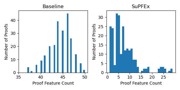
(a) For MNIST Dataset

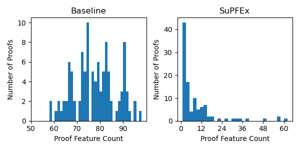
(b) For CIFAR-10 dataset

Figure 1: Distribution of the size of the proof feature set computed by SuPFEx Algorithm on COLT-trained networks.

is better than the size of the proof feature set extracted by the trivial algorithm - one that only removes only “zero” features which include the proof features ($[l,u]$) where both $l=u=0$. (Definition 1) For each network, we use $500$ randomly picked images from their corresponding test sets. The $\epsilon$ used for MNIST networks is $0.02$ and that for CIFAR-10 networks is $0.2/255$. We note that although the robustly trained networks can be verified robust for higher values of $\epsilon$, it is not possible to verify standard networks with such high values. To achieve common ground, we use small $\epsilon$ values for experiments involving standard networks and conduct separate experiments on only robustly trained networks with higher values of $\epsilon$ ($0.1$ for MNIST, $2/255$ for CIFAR-10 networks). As shown in Table 1 we do not observe any significant change in the performance of SuPFEx w.r.t different $\epsilon$-values.
In Table 1, we show the value of $\epsilon$ used to define the region $\phi$ in column 3, and the total number of properties proved out of 500 in column 4. The size of the original proof feature size corresponding to each network is shown in column 5, the mean and median of the proof feature set size computed using Theorem 4.2 in columns 6 and 7 respectively, and the mean and median of the proof feature set size computed using SuPFEx in columns 8 and 9 respectively. We note that feature sets obtained by SuPFEx are significantly smaller than the upper bound provided by Theorem 4.2. For example, in the case of the PGD trained MNIST network with $1000$ neurons in the penultimate layer, the average size computed from Theorem 4.2 is $218.02$, while that obtained using SuPFEx is only $5.57$. In the last two columns of Table 1, we summarise the percentage of cases where we are able to achieve a proof feature set of size less than or equal to $5$ and $10$ respectively. Figures 1(a) and 1(b) display a histogram where the x-axis is the size of the extracted proof feature set using SuPFEx and y-axis is the number of local robustness properties for COLT-trained DNNs. Histograms for other DNNs are presented in Appendix B. These histograms are skewed towards the left which means that for most of the local properties, we are able to generate a small set of proof features using SuPFEx .

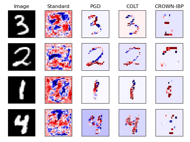
(a) Gradient maps generated on MNIST networks.

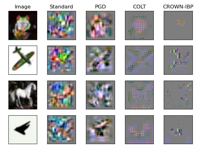
(b) Gradient maps generated on CIFAR-10 networks.

Figure 2: The top proof feature corresponding to DNNs trained using different methods rely on different input features.

5.3 Qualititive comparison of robustness proofs

It has been observed in (Tsipras et al., 2019) that the standardly trained networks rely on some of the spurious features in the input in order to gain a higher accuracy and as a result, are not very robust against adversarial attacks. On the other hand, the empirically robustly trained networks rely more on human-understandable features and are, therefore, more robust against attacks. This empirical robustness comes at cost of reduced accuracy. So, there is an inherent dissimilarity between the types of input features that the standard and adversarially trained networks rely on while classifying a single input. Also, certified robust trained networks are even more robust than the empirically trained ones, however, they report even less accuracy (Müller et al., 2021). In this section, we interpret proof features obtained with SuPFEx and use these interpretations to qualitatively check whether the dissimilarities are also evident in the invariants captured by the different proofs of the same robustness property on standard and robustly trained networks. We also study the effect of certified robust training methods like CROWN-IBP (Zhang et al., 2020), empirically robust training methods like PGD (Madry et al., 2018) and training methods that combine both adversarial and certified training like COLT (Balunovic & Vechev, 2020) on the proof features.
For a local input region $\phi$, we say that a robustness proof is semantically meaningful if it focuses on the relevant features of the output class for images contained inside $\phi$ and not on the spurious features. In the case of MNIST or CIFAR-10 images, spurious features are the pixels that form a part of the background of the image, whereas important features are the pixels that are a part of the actual object being identified by the network. Gradient map of the extracted proof features w.r.t. to the input region $\phi$ gives us an idea of the input pixels that the network focuses on. We obtain the gradient maps by calculating the mean gradient over 100 uniformly drawn samples from $\phi$ as described in Section 4.3. As done in (Tsipras et al., 2019), to avoid introducing any inherent bias in proof feature visualization, no preprocessing (other than scaling and clipping for visualization) is applied to the gradients obtained for each individual sample.
In Fig. 2, we compare the gradient maps corresponding to the top proof feature (the one having the highest priority $P_{ub}(\mathcal{F}_{n_{i}})$) on networks from Table 1 on representative images of different output classes in the MNIST and CIFAR10 test sets. The experiments leads us to interesting observations - even if some property is verified for both the standard network and the robustly trained network, there is a difference in the human interpretability of the types of input features that the proofs rely on. The standard networks and the provably robust trained networks like CROWN-IBP are the two extremes of the spectrum. For the networks obtained with standard training, we observe that although the top-proof feature does depend on some of the semantically meaningful regions of the input image, the gradient at several spurious features is also non-zero. On the other hand, the top proof feature corresponding to state-of-the-art provably robust training method CROWN-IBP filters out most of the spurious features, but it also misses out on some meaningful features. The proofs of PGD-trained networks filter out the spurious features and are, therefore, more semantically aligned than the standard networks. The proofs of the training methods that combine both empirical robustness and provable robustness like COLT in a way provide the best of both worlds by not only selectively filtering out the spurious features but also highlighting the more human interpretable features, unlike the certifiably trained networks. So, as the training methods tend to regularize more for robustness, their proofs become more conservative in relying on the input features. To further support our observation, we show additional plots for the top proof feature visualization in Appendix B.2 and visualization for multiple proof features in Appendix B.4. We also conduct experiments for different values of $\epsilon$ used for defining $\phi$. The extracted proof features set w.r.t high $\epsilon$ values ($\epsilon=0.1$ for MNIST and $\epsilon=2/255$ for CIFAR-10) are similar to those generated with smaller $\epsilon$. The gradient maps corresponding to the top feature for higher $\epsilon$ values are also similar as shown in Appendix B.3. For COLT-trained MNIST networks, in  B.5 we compare the gradients of top proof features retained by SuPFEx with the pruned proof features with low priority. As expected, graidents of the pruned proof features with low priority contain spurious input features.

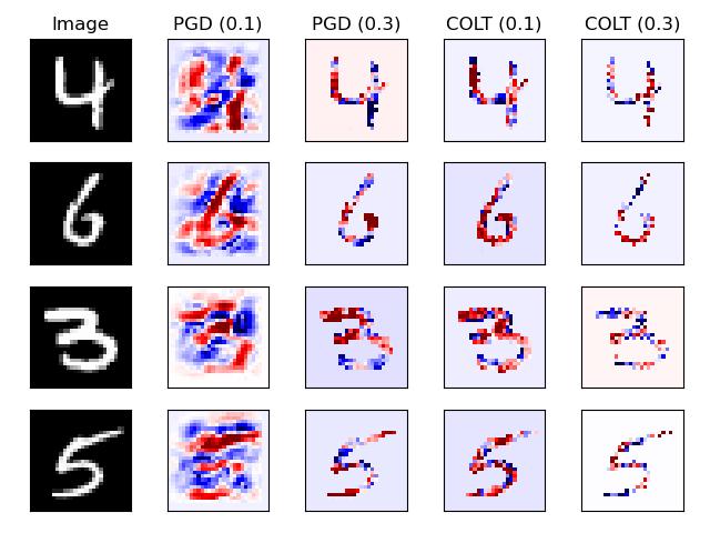
Figure 3: Visualization of gradients of the top proof feature for PGD and COLT networks trained using different values of $\epsilon_{train}$.

5.4 Sensitivity analysis on training parameters

It is expected that DNNs trained with larger $\epsilon_{train}$ values are more robust. So, we analyze the sensitivity of the extracted proof features to $\epsilon_{train}$. We use the DNNs trained with PGD and COLT and $\epsilon_{train}\in\{0.1,0.3\}$ on the MNIST dataset. Fig 3 visualize proof features for the DNNs with additional plots are available in Appendix B.6. We observe that by increasing the value of $\epsilon_{train}$, the top proof feature filters out more input features. This is aligned with our observation in Section 5.3 that a more robustly trained neural networks are more conservative in using the input features.

5.5 Comparing proofs of different verifiers

The proof features extracted by SuPFEx are specific to the proof generated by the verifier. In this experiment, we compare proof features generated by two popular verifiers IBP (Zhang et al., 2020; an, 2018) and DeepZ on networks shown in Table 1 for the same properties as before. Note that, although IBP is computationally efficient, it is less precise than DeepZ. For standard DNNs, most of the properties cannot be proved by IBP. Hence, in this experiment, we omit standard DNNs and also, consider only the properties that can be verified by both DeepZ and IBP. Table 2 presents the % cases where the top proof feature computed by both the verifiers is the same (column 2), the % cases where the top 5 proof features computed by both the verifiers are the same and the % cases where the complete proof feature sets computed by both the verifiers are same. We observe that for the MNIST dataset, in 100% of the cases for PGD-trained and COLT-trained networks and in 99.79% cases for the CROWN-IBP trained networks, the top feature computed by both the verifiers is the same. Detailed table is available in Appendix B.7.

6 Conclusion

In this work, we develop a novel method called SuPFEx to interpret neural network robustness proofs. We empirically establish that even if a property holds for a DNN, the proof for the property may rely on spurious or semantically meaningful features depending on the training method used to train the DNNs. We believe that SuPFEx can be applied for diagnosing the trustworthiness of DNNs inside their development pipeline.

Table 2: Comparing proofs of IBP & DeepZ

Training	% proofs with the		% proofs with the		% proofs with the
Method	same top feature		same top-5 feature		same feature set
	MNIST	CIFAR10	MNIST	CIFAR10	MNIST	CIFAR10
PGD Trained	100 %	100 %	92.0 %	98.31 %	92.0 %	96.87 %
COLT	100 %	97.87 %	87.17 %	92.53 %	82.05 %	89.36 %
CROWN-IBP	99.79 %	100 %	96.26 %	97.92 %	93.15 %	95.89 %

Appendix A Mathematical proofs

Theorem 4.2: If the verifier $\mathcal{V}$ can prove the property $(\phi,\psi)$ on the network $N$, then $\mathcal{F}_{S_{0}}^{(\mathbb{A})}$ computed by Algorithm 1 is sufficient (Definition 4.1).

Proof.

By induction on the number of steps of the while loop.
Induction Hypothesis: At each step of the loop, $\mathcal{F}^{\mathbb{(A)}}_{S_{0}}\cup\mathcal{F}^{\mathbb{(A)}}_{S}$ is sufficient.
Base Case: At step 0, i.e., at initialization, $\mathcal{F}^{\mathbb{(A)}}_{S_{0}}=\{\}$ and $\mathcal{F}^{\mathbb{(A)}}_{S}\mathcal{F}$. So, $\mathcal{F}^{\mathbb{(A)}}_{S_{0}}\cup\mathcal{F}^{\mathbb{(A)}}_{S}=\mathcal{F}$. Given that $\mathcal{V}$ proves the property $(\phi,\psi)$ on $N$, from Definition 4.1, $\mathcal{F}$ is sufficient.
Induction Case: Let $\mathcal{F}^{\mathbb{(A)}}_{S_{0}}\cup\mathcal{F}^{\mathbb{(A)}}_{S}$ be sufficient for $n$-th step of the loop. Consider the following cases for $(n+1)$-th step of the loop.

1. Let $\mathcal{F}^{\mathbb{(A)}}_{S_{0}}\cup\mathcal{F}^{\mathbb{(A)}}_{S_{1}}$ be sufficient at line 12. In this case, $\mathcal{F}^{\mathbb{{A}}}_{S}$ is updated by $\mathcal{F}^{\mathbb{(A)}}_{S_{1}}$ (line 14). So, $\mathcal{F}^{\mathbb{(A)}}_{S_{0}}\cup\mathcal{F}^{\mathbb{(A)}}_{S}$ is sufficient.

2. Let $\mathcal{F}^{\mathbb{(A)}}_{S_{0}}\cup\mathcal{F}^{\mathbb{(A)}}_{S_{1}}$ be not sufficient at line 12. In this case, $\mathcal{F}^{\mathbb{(A)}}_{S_{0}}$ and $\mathcal{F}^{\mathbb{(A)}}_{S}$ are updated as in lines 16 and 17. Let the new $\mathcal{F}^{\mathbb{(A)}}_{S_{0}}$ and $\mathcal{F}^{\mathbb{(A)}}_{S}$ be $\mathcal{F}^{\prime\mathbb{(A)}}_{S_{0}}$ and $\mathcal{F}^{\prime\mathbb{(A)}}_{S}$. So, $\mathcal{F}^{\prime\mathbb{(A)}}_{S_{0}}=\mathcal{F}^{\mathbb{(A)}}_{S_{0}}\cup\mathcal{F}^{\mathbb{(A)}}_{S_{1}}$ and $\mathcal{F}^{\prime\mathbb{(A)}}_{S}=\mathcal{F}^{\mathbb{(A)}}_{S_{2}}$. So, $\mathcal{F}^{\prime\mathbb{(A)}}_{S_{0}}\cup\mathcal{F}^{\prime\mathbb{(A)}}_{S}=\mathcal{F}^{\mathbb{(A)}}_{S_{0}}\cup\mathcal{F}^{\mathbb{(A)}}_{S_{1}}\cup\mathcal{F}^{\mathbb{(A)}}_{S_{2}}$. Also, $\mathcal{F}^{\mathbb{(A)}}_{S_{1}}\cup\mathcal{F}^{\mathbb{(A)}}_{S_{2}}=\mathcal{F}^{\mathbb{(A)}}_{S}$. So, $\mathcal{F}^{\prime\mathbb{(A)}}_{S_{0}}\cup\mathcal{F}^{\prime\mathbb{(A)}}_{S}=\mathcal{F}^{\mathbb{(A)}}_{S_{0}}\cup\mathcal{F}^{\mathbb{(A)}}_{S}$. So, from induction hypothesis, $\mathcal{F}^{\prime\mathbb{(A)}}_{S_{0}}\cup\mathcal{F}^{\prime\mathbb{(A)}}_{S}$ is sufficient.

∎

$\forall\mathcal{F}_{S}\subseteq\mathcal{F}$, $\delta(\mathcal{F}_{S})\leq\sum\limits_{\mathcal{F}_{n_{i}}\in\mathcal{F}\setminus\mathcal{F}_{S}}P_{ub}(\mathcal{F}_{n_{i}})$ where $P_{ub}(\mathcal{F}_{n_{i}})$ is defined in  (4).

Proof.

$$\delta(\mathcal{F}_{S}) =|\Lambda(\mathcal{A})-\Lambda(\mathcal{A}(W_{l},S))|$$

$$=\max_{X\in\mathcal{A}_{l-1}}|\sum\limits_{\mathcal{F}_{n_{i}}\in\mathcal{F}\setminus\mathcal{F}_{S}}C^{T}W[:i]X|$$

$$\leq\max_{X\in\mathcal{A}_{l-1}}\sum\limits_{\mathcal{F}_{n_{i}}\in\mathcal{F}\setminus\mathcal{F}_{S}}|C^{T}W[:i]X|$$

$$\leq\sum\limits_{\mathcal{F}_{n_{i}}\in\mathcal{F}\setminus\mathcal{F}_{S}}\max_{X\in\mathcal{A}_{l-1}}|C^{T}W[:i]X|$$

$$=\sum\limits_{\mathcal{F}_{n_{i}}\in\mathcal{F}\setminus\mathcal{F}_{S}}P_{ub}(\mathcal{F}_{n_{i}})\quad[\text{ From }~{}\eqref{eq:apxpriority}]$$

∎

A feature set $\mathcal{F}_{S}\subseteq\mathcal{F}$ with $\delta(\mathcal{F}_{S})\leq\Lambda(\mathcal{A})$ is sufficient provided $\Lambda(\mathcal{A})\geq 0$.

Proof.

$\delta(\mathcal{F}_{S})=|\Lambda(\mathcal{A})-\Lambda(\mathcal{A}(W_{l},S))|$. So, there can be two cases:

1. $\Lambda(\mathcal{A}(W_{l},S))=\Lambda(\mathcal{A})+\delta(\mathcal{F}_{S})$. Since, $\Lambda(\mathcal{A})\geq 0$ and $\delta(\mathcal{F}_{S})\geq 0$, $\Lambda(\mathcal{A}(W_{l},S))\geq 0$. So, $\mathcal{F}_{S}$ is sufficient.

2. $\Lambda(\mathcal{A}(W_{l},S))=\Lambda(\mathcal{A})-\delta(\mathcal{F}_{S})$
   $\Lambda(\mathcal{A})\geq 0$ and $\delta(\mathcal{F}_{S})\leq\Lambda(\mathcal{A})$.
   So, $\Lambda(\mathcal{A}(W_{l},S))\geq 0$. So, $\mathcal{F}_{S}$ is sufficient.

∎

Let, $P_{max}$ denote the maximum of all priorities $P_{ub}(\mathcal{F}_{n_{i}})$ over $\mathcal{F}$.
Let $\mathcal{F}_{S}\subseteq\mathcal{F}$. If $|\mathcal{F}_{S}|\leq\lfloor\frac{\Lambda(\mathcal{A})}{P_{max}}\rfloor$, then proof feature set $\mathcal{F}_{S}^{c}=\mathcal{F}\setminus\mathcal{F}_{S}$ is sufficient provided $\Lambda(\mathcal{A})\geq 0$.

Proof.

$$\;\forall\mathcal{F}_{n_{i}}\in\mathcal{F},P_{ub}(\mathcal{F}_{n_{i}})\leq P_{max}$$

From Lemma A, $$\;\delta(\mathcal{F}_{S}^{c})\leq|\mathcal{F}_{S}|\times P_{max}$$

Also, $$\;|\mathcal{F}_{S}|\leq\lfloor\frac{\Lambda(\mathcal{A})}{P_{max}}\rfloor$$

So, $$\;\delta(\mathcal{F}_{S}^{c})\leq\Lambda(\mathcal{A})$$

From Lemma A, $$\;\mathcal{F}_{S}^{c}\text{ is sufficient.}$$

∎

Theorem 4.2: Given any network $N$ is verified on $(\phi,\psi)$ with verifier $\mathcal{V}$ then $|\mathcal{F}_{S_{0}}^{(\mathbb{A})}|\leq d_{l-1}-|Z(\mathcal{F})|-\lfloor\frac{\Lambda(\mathcal{A})}{P_{max}}\rfloor$

Proof.

The algorithm 1 arranges the elements of the proof feature set $\mathcal{F}$ in decreasing order according to the priority defined by $P_{ub}$.
Let $\mathcal{F}^{\prime}$ be the ordered set corresponding to $\mathcal{F}$. So, $\mathcal{F}^{\prime}=\mathcal{F}_{n_{1}}::\cdots::\mathcal{F}_{n_{m}}$, where $::$ is the list concatenation.
The elements of $Z(\mathcal{F})$ will be at the end of this ordering. So, $\mathcal{F}^{\prime}$ can be written as $\mathcal{F}^{\prime\prime}::Z(\mathcal{F})$ where $Z(\mathcal{F})=\mathcal{F}_{n_{k+1}}::\cdots::\mathcal{F}_{n_{m}}$ and $\mathcal{F}^{\prime\prime}=\mathcal{F}_{n_{1}}::\cdots::\mathcal{F}_{n_{k}}$ and $p$ be some of the last elements of $\mathcal{F}^{\prime\prime}$ s.t. the sum of their priorities just less than $\lfloor\frac{\Lambda(\mathcal{A})}{P_{max}}\rfloor$, i.e.,

$$p=\mathcal{F}_{n_{j}}::\cdots::\mathcal{F}_{n_{k}}$$

$$\sum\limits_{i=j}^{k}P_{ub}(\mathcal{F}_{n_{i}})\leq\lfloor\frac{\Lambda(\mathcal{A})}{P_{max}}\rfloor$$

$$\sum\limits_{i=j-1}^{k}P_{ub}(\mathcal{F}_{n_{i}})\geq\lfloor\frac{\Lambda(\mathcal{A})}{P_{max}}\rfloor$$

Further, let $p^{\prime}=p::Z(\mathcal{F})$, i.e., $p^{\prime}=\mathcal{F}_{n_{j}}::\cdots::\mathcal{F}_{n_{m}}$. Since $P_{ub}$ is 0 for all elements of $Z(\mathcal{F})$,

$$\sum\limits_{i=j}^{m}P_{ub}(\mathcal{F}_{n_{i}})\leq\lfloor\frac{\Lambda(\mathcal{A})}{P_{max}}\rfloor$$ (5)

Also, $|p^{\prime}|=|Z(\mathcal{F})|+\lfloor\frac{\Lambda(\mathcal{A})}{P_{max}}\rfloor$ Now, we prove by induction on the number of steps of the while loop in the algorithm 1 that the set $\mathcal{F}_{S_{0}}^{(\mathbb{A})}$ never contains any elements from $p^{\prime}$.
Induction Hypothesis: $\mathcal{F}_{S_{0}}^{(\mathbb{A})}\cap p^{\prime}=\{\}$
Base Case: At initialization, $\mathcal{F}_{S_{0}}^{(\mathbb{A})}=\{\}$. So, the induction hypothesis holds trivially.
Induction Step: Let the induction hypothesis be true for the $n$-th step of the algorithm 1. For the $(n+1)$-th step, let the new $\mathcal{F}^{\mathbb{(A)}}_{S_{0}}$ and $\mathcal{F}^{\mathbb{(A)}}_{S}$ be $\mathcal{F}^{\prime\mathbb{(A)}}_{S_{0}}$ and $\mathcal{F}^{\prime\mathbb{(A)}}_{S}$ respectively. Consider the following two cases:

1. Let $\mathcal{F}^{\mathbb{(A)}}_{S_{0}}\cup\mathcal{F}^{\mathbb{(A)}}_{S_{1}}$ be sufficient at line 12. In this case, $\mathcal{F}^{\prime\mathbb{{A}}_{S_{0}}}=\mathcal{F}^{\mathbb{{A}}_{S_{0}}}$. So, the induction hypothesis holds.

2. Let $\mathcal{F}^{\mathbb{(A)}}_{S_{0}}\cup\mathcal{F}^{\mathbb{(A)}}_{S_{1}}$ be not sufficient at line 12.
   Claim: $\mathcal{F}^{\mathbb{(A)}}_{S_{0}}\cap p^{\prime}=\{\}$
   Let the above claim be false.
   $\implies\mathcal{F}^{\mathbb{(A)}}_{S_{0}}\cap p^{\prime}\not=\{\}$
   $\implies\mathcal{F}\setminus(\mathcal{F}^{\mathbb{(A)}}_{S_{0}}\cup\mathcal{F}^{\mathbb{(A)}}_{S_{1}})\subset p^{\prime}$
   $\implies\sum\limits_{\mathcal{F}{n_{i}}\in\mathcal{F}\setminus(\mathcal{F}^{\mathbb{(A)}}_{S_{0}}\cup\mathcal{F}^{\mathbb{(A)}}_{S_{1}})}P_{ub}<\lfloor\frac{\Lambda(\mathcal{A})}{P_{max}}\rfloor\quad$[From (6)]
   $\implies(\mathcal{F}^{\mathbb{(A)}}_{S_{0}}\cup\mathcal{F}^{\mathbb{(A)}}_{S_{1}})$ is sufficient. (From Lemma A)
   $\implies$ Contradiction.
   So, $\mathcal{F}^{\mathbb{(A)}}_{S_{1}}\cap p^{\prime}=\{\}$. In this step, $\mathcal{F}^{\prime\mathbb{(A)}}_{S_{0}}=\mathcal{F}^{\mathbb{(A)}}_{S_{0}}\cup\mathcal{F}^{\mathbb{(A)}}_{S_{1}}$. Also, from induction hypothesis, $\mathcal{F}^{\mathbb{(A)}}_{S_{0}}\cap p^{\prime}=\{\}$. Therefore, the induction hypothesis holds, i.e., $\mathcal{F}^{\prime\mathbb{(A)}}_{S_{0}}\cap p^{\prime}=\{\}$.

∎

Appendix B Additional Experiments

B.1 Plots for distributions of the size of proof feature set

Table 3: Distribution of the size of proof feature set for Standardly trained networks on MNIST dataset

$\boldsymbol{\epsilon}$	MNIST
0.02
0.1

Table 4: Distribution of the size of proof feature set for Standardly trained networks on CIFAR-10 dataset

$\boldsymbol{\epsilon}$	CIFAR-10
$\mathbf{\frac{0.2}{255}}$
$\mathbf{\frac{0.2}{255}}$

Table 5: Distribution of the size of proof feature set for MNIST dataset

Training Method	$\mathbf{\boldsymbol{\epsilon}=0.02}$	$\mathbf{\boldsymbol{\epsilon}=0.1}$
PGD
COLT
CROWN-IBP

Table 6: Distribution of the size of proof feature set for CIFAR-10 dataset

Training Method	$\mathbf{\boldsymbol{\epsilon}=0.2/255}$	$\mathbf{\boldsymbol{\epsilon}=2/255}$
PGD
COLT
CROWN-IBP

B.2 Additional plots for the top proof feature visualization

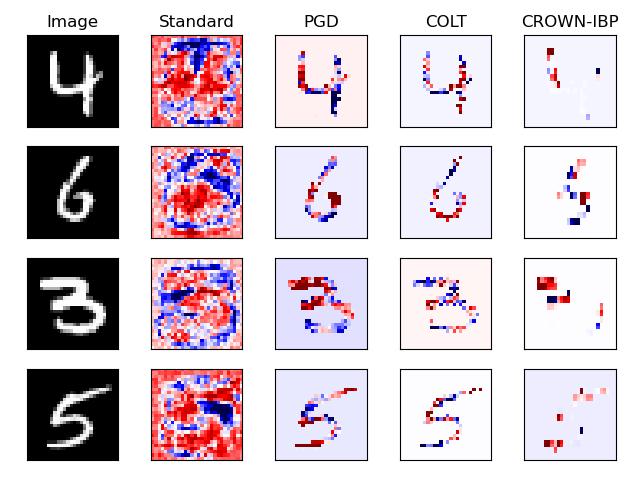
(a) Gradient maps generated on MNIST networks

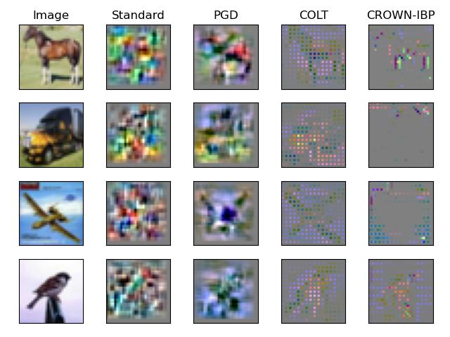
(b) Gradient maps generated on CIFAR-10 networks

Figure 4: Additional plots for the top proof feature visualization (in addition to Fig. 2) - Visualization of gradient map of top proof feature (having highest priority) generated for networks trained with different training methods. It is evident that the top proof feature corresponding to the standard network highlights both relevant and spurious input features. In contrast, the top proof feature of the provably robust network does filter out the spurious input features, but it comes at the expanse of some important input features. The top proof features of the networks trained with PGD filter out more spurious features as compared to standard networks. Finally, the top proof features of the networks trained with COLT filter out the spurious input features and also correctly highlight the relevant input features.

B.3 Visualization of the top proof feature for higher $\epsilon$ values

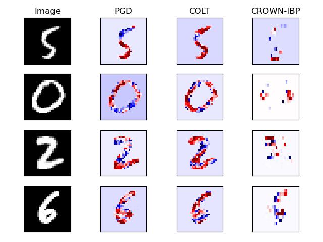
(a) Gradient maps generated on MNIST networks

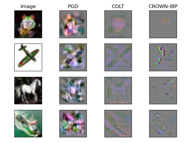
(b) Gradient maps generated on CIFAR-10 networks

Figure 5: Visualization of gradient map of top proof feature (having highest priority) generated for networks trained with different robust training methods. For these networks, we define local properties with higher $\epsilon$ values. For MNIST networks and CIFAR-10 networks, we take $\epsilon=0.1$ and $\epsilon=2/255$ respectively.

B.4 Visualization of multiple proof features from the extracted proof feature set

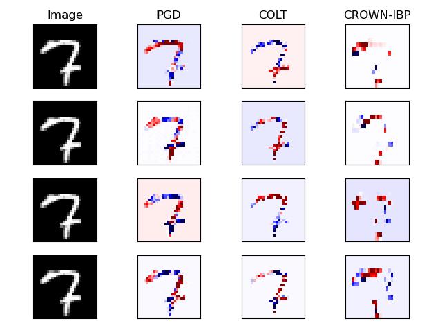
(a) Gradient maps generated on MNIST networks

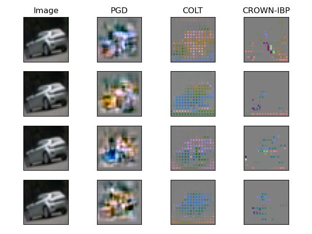
(b) Gradient maps generated on CIFAR-10 networks

Figure 6: Visualization of gradient maps of top-4 proof features (having highest priority) extracted for networks trained with different robust training methods. The gradient maps of the proof features are presented in decreasing order of priority with the top row showing the gradient map corresponding to the top proof feature of each network.

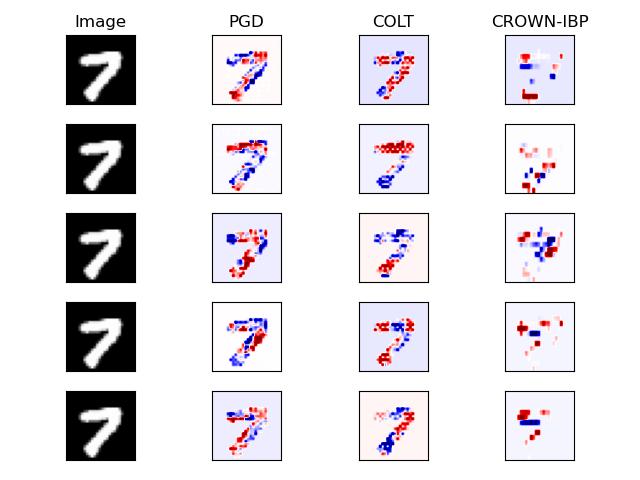
(a) Gradient maps generated on MNIST networks

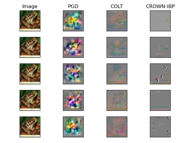
(b) Gradient maps generated on CIFAR-10 networks

Figure 7: Visualization of gradient maps of top-5 proof features (having highest priority) extracted for networks trained with different robust training methods. The gradient maps of the proof features are presented in decreasing order of priority with the top row showing the gradient map corresponding to the top proof feature of each network.

B.5 Comparing proof features with high priority to pruned proof features with low priority

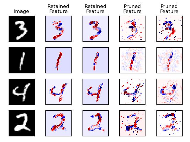
Figure 8: Comparing gradients of the top proof features retained by SuPFEx to proof features with low priority. As expected, proof features with low priority contain spurious input features. The shown gradients are computed on COLT-trained MNIST networks.

B.6 Additional plots for sensitivity analysis w.r.t $\boldsymbol{\epsilon_{train}}$

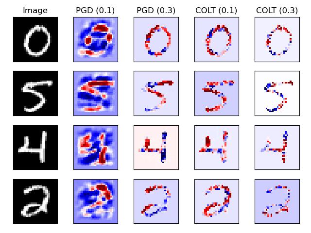
Figure 9: Additional plots for visualizing gradients of the top proof feature for PGD and COLT networks trained using different values of $\epsilon_{train}\in\{0.1,0.3\}$ The gradient map corresponding to the networks trained with the higher value of $\epsilon_{train}$ filter out more input features than the ones trained with smaller $\epsilon_{train}$ value.

B.7 Comparing proofs of different verifiers

We note that for high values of $\epsilon$ i.e. $\epsilon=0.1$ for MNIST and $\epsilon=2/255$ for CIFAR-10 most of the properties don’t get verified even for robustly trained networks with IBP. Hence, we omitted them for this analysis.

Table 7: Comparing proofs of IBP & DeepZ

Dataset	Training	Input	% properties	% properties	% proofs with the	% proofs with the	% proofs with the
	Method	Region $(\phi)$	proved by IBP	proved by DeepZ	same top feature	same top-5 feature	same feature set
		eps ($\epsilon$)
MNIST	PGD Trained	0.02	26.0 %	82.0 %	100 %	92.0 %	92.0 %
	COLT	0.02	49.8 %	89.4 %	100.0 %	87.17 %	82.05 %
	CROWN-IBP	0.02	93.4 %	96.4 %	99.79 %	96.26 %	93.15 %
CIFAR-10	PGD Trained	0.2/255	10.2 %	47.0 %	100 %	98.31 %	96.87 %
	COLT	0.2/255	17.2 %	53.0 %	97.87 %	92.53 %	89.36 %
	CROWN-IBP	0.2/255	21.8 %	53.0 %	100 %	97.92 %	95.89 %

References

- Amato et al. (2013) Amato, F., López, A., Peña-Méndez, E. M., Vaňhara, P., Hampl, A., and Havel, J. Artificial neural networks in medical diagnosis. Journal of Applied Biomedicine, 11(2), 2013.
- an (2018) an, S. G. On the effectiveness of interval bound propagation for training verifiabl. ArXiv preprint, abs/1810.12715, 2018.
- Anderson et al. (2020) Anderson, R., Huchette, J., Ma, W., Tjandraatmadja, C., and Vielma, J. P. Strong mixed-integer programming formulations for trained neural networks. Mathematical Programming, 2020.
- Bak et al. (2020) Bak, S., Tran, H., Hobbs, K., and Johnson, T. T. Improved geometric path enumeration for verifying relu neural networks. In Lahiri, S. K. and Wang, C. (eds.), Computer Aided Verification - 32nd International Conference, CAV 2020, Los Angeles, CA, USA, July 21-24, 2020, Proceedings, Part I, volume 12224 of Lecture Notes in Computer Science, pp. 66–96. Springer, 2020. doi: 10.1007/978-3-030-53288-8“˙4. URL https://doi.org/10.1007/978-3-030-53288-8_4.
- Balunovic & Vechev (2020) Balunovic, M. and Vechev, M. T. Adversarial training and provable defenses: Bridging the gap. In 8th International Conference on Learning Representations, ICLR 2020, Addis Ababa, Ethiopia, April 26-30, 2020. OpenReview.net, 2020.
- Bau et al. (2020) Bau, D., Zhu, J.-Y., Strobelt, H., Lapedriza, A., Zhou, B., and Torralba, A. Understanding the role of individual units in a deep neural network. Proceedings of the National Academy of Sciences, 117(48):30071–30078, 2020.
- Bojarski et al. (2016) Bojarski, M., Del Testa, D., Dworakowski, D., Firner, B., Flepp, B., Goyal, P., Jackel, L. D., Monfort, M., Muller, U., Zhang, J., et al. End to end learning for self-driving cars. arXiv preprint arXiv:1604.07316, 2016.
- Bunel et al. (2020a) Bunel, R., Lu, J., Turkaslan, I., Kohli, P., Torr, P., and Mudigonda, P. Branch and bound for piecewise linear neural network verification. Journal of Machine Learning Research, 21(2020), 2020a.
- Bunel et al. (2020b) Bunel, R. R., Hinder, O., Bhojanapalli, S., and Dvijotham, K. An efficient nonconvex reformulation of stagewise convex optimization problems. Advances in Neural Information Processing Systems, 33, 2020b.
- Carlini & Wagner (2017) Carlini, N. and Wagner, D. Towards evaluating the robustness of neural networks. In 2017 ieee symposium on security and privacy (sp), pp. 39–57. Ieee, 2017.
- Cohen et al. (2019) Cohen, J., Rosenfeld, E., and Kolter, Z. Certified adversarial robustness via randomized smoothing. In Chaudhuri, K. and Salakhutdinov, R. (eds.), Proceedings of the 36th International Conference on Machine Learning, volume 97 of Proceedings of Machine Learning Research, pp. 1310–1320. PMLR, 09–15 Jun 2019. URL https://proceedings.mlr.press/v97/cohen19c.html.
- Ehlers (2017) Ehlers, R. Formal verification of piece-wise linear feed-forward neural networks. In International Symposium on Automated Technology for Verification and Analysis, 2017.
- Ferrari et al. (2022) Ferrari, C., Mueller, M. N., Jovanović, N., and Vechev, M. Complete verification via multi-neuron relaxation guided branch-and-bound. In International Conference on Learning Representations, 2022. URL https://openreview.net/forum?id=l_amHf1oaK.
- Fromherz et al. (2021) Fromherz, A., Leino, K., Fredrikson, M., Parno, B., and Pasareanu, C. Fast geometric projections for local robustness certification. In International Conference on Learning Representations, 2021. URL https://openreview.net/forum?id=zWy1uxjDdZJ.
- Gehr et al. (2018) Gehr, T., Mirman, M., Drachsler-Cohen, D., Tsankov, P., Chaudhuri, S., and Vechev, M. Ai2: Safety and robustness certification of neural networks with abstract interpretation. In 2018 IEEE Symposium on Security and Privacy (SP), 2018.
- Goyal et al. (2019) Goyal, Y., Wu, Z., Ernst, J., Batra, D., Parikh, D., and Lee, S. Counterfactual visual explanations. In International Conference on Machine Learning, pp. 2376–2384. PMLR, 2019.
- Hsieh et al. (2021) Hsieh, C.-Y., Yeh, C.-K., Liu, X., Ravikumar, P. K., Kim, S., Kumar, S., and Hsieh, C.-J. Evaluations and methods for explanation through robustness analysis. In International Conference on Learning Representations, 2021. URL https://openreview.net/forum?id=4dXmpCDGNp7.
- Kim et al. (2016) Kim, B., Khanna, R., and Koyejo, O. O. Examples are not enough, learn to criticize! criticism for interpretability. Advances in neural information processing systems, 29, 2016.
- Koh & Liang (2017) Koh, P. W. and Liang, P. Understanding black-box predictions via influence functions. In International conference on machine learning, pp. 1885–1894. PMLR, 2017.
- Krizhevsky (2009) Krizhevsky, A. Learning multiple layers of features from tiny images. 2009.
- LeCun et al. (1989) LeCun, Y., Boser, B. E., Denker, J. S., Henderson, D., Howard, R. E., Hubbard, W. E., and Jackel, L. D. Handwritten digit recognition with a back-propagation network. In NIPS, pp. 396–404, 1989.
- Liao & Cheung (2022) Liao, Z. and Cheung, M. Automated invariance testing for machine learning models using sparse linear layers. In ICML 2022: Workshop on Spurious Correlations, Invariance and Stability, 2022. URL https://openreview.net/forum?id=VP8ATzLGyQx.
- Madry et al. (2018) Madry, A., Makelov, A., Schmidt, L., Tsipras, D., and Vladu, A. Towards deep learning models resistant to adversarial attacks. In Proc. International Conference on Learning Representations (ICLR), 2018.
- Mazzucato & Urban (2021) Mazzucato, D. and Urban, C. Reduced products of abstract domains for fairness certification of neural networks. In Dragoi, C., Mukherjee, S., and Namjoshi, K. S. (eds.), Static Analysis - 28th International Symposium, SAS 2021, Chicago, IL, USA, October 17-19, 2021, Proceedings, volume 12913 of Lecture Notes in Computer Science, pp. 308–322. Springer, 2021. doi: 10.1007/978-3-030-88806-0“˙15. URL https://doi.org/10.1007/978-3-030-88806-0_15.
- Müller et al. (2021) Müller, C., Serre, F., Singh, G., Püschel, M., and Vechev, M. Scaling polyhedral neural network verification on gpus. In Smola, A., Dimakis, A., and Stoica, I. (eds.), Proceedings of Machine Learning and Systems, volume 3, pp. 733–746, 2021. URL https://proceedings.mlsys.org/paper/2021/file/ca46c1b9512a7a8315fa3c5a946e8265-Paper.pdf.
- Palma et al. (2021) Palma, A. D., Behl, H. S., Bunel, R. R., Torr, P. H. S., and Kumar, M. P. Scaling the convex barrier with active sets. In 9th International Conference on Learning Representations, ICLR 2021, Virtual Event, Austria, May 3-7, 2021, 2021.
- Ribeiro et al. (2016) Ribeiro, M. T., Singh, S., and Guestrin, C. ” why should i trust you?” explaining the predictions of any classifier. In Proceedings of the 22nd ACM SIGKDD international conference on knowledge discovery and data mining, pp. 1135–1144, 2016.
- Salman et al. (2019) Salman, H., Yang, G., Zhang, H., Hsieh, C., and Zhang, P. A convex relaxation barrier to tight robustness verification of neural networks. In Advances in Neural Information Processing Systems 32: Annual Conference on Neural Information Processing Systems 2019, NeurIPS 2019, December 8-14, 2019, Vancouver, BC, Canada, 2019.
- Simonyan et al. (2014) Simonyan, K., Vedaldi, A., and Zisserman, A. Deep inside convolutional networks: Visualising image classification models and saliency maps. In Bengio, Y. and LeCun, Y. (eds.), 2nd International Conference on Learning Representations, ICLR 2014, Banff, AB, Canada, April 14-16, 2014, Workshop Track Proceedings, 2014. URL http://arxiv.org/abs/1312.6034.
- Singh et al. (2018) Singh, G., Gehr, T., Mirman, M., Püschel, M., and Vechev, M. Fast and effective robustness certification. Advances in Neural Information Processing Systems, 31, 2018.
- Singh et al. (2019a) Singh, G., Ganvir, R., Püschel, M., and Vechev, M. Beyond the single neuron convex barrier for neural network certification. In Advances in Neural Information Processing Systems, 2019a.
- Singh et al. (2019b) Singh, G., Gehr, T., Püschel, M., and Vechev, M. An abstract domain for certifying neural networks. Proceedings of the ACM on Programming Languages, 3(POPL), 2019b.
- Singh et al. (2019c) Singh, G., Gehr, T., Püschel, M., and Vechev, M. Robustness certification with refinement. In International Conference on Learning Representations, 2019c. URL https://openreview.net/forum?id=HJgeEh09KQ.
- Smilkov et al. (2017) Smilkov, D., Thorat, N., Kim, B., Viégas, F. B., and Wattenberg, M. Smoothgrad: removing noise by adding noise. CoRR, abs/1706.03825, 2017. URL http://arxiv.org/abs/1706.03825.
- Sundararajan et al. (2017) Sundararajan, M., Taly, A., and Yan, Q. Axiomatic attribution for deep networks. In International conference on machine learning, pp. 3319–3328. PMLR, 2017.
- Tsipras et al. (2019) Tsipras, D., Santurkar, S., Engstrom, L., Turner, A., and Madry, A. Robustness may be at odds with accuracy. In International Conference on Learning Representations, 2019. URL https://openreview.net/forum?id=SyxAb30cY7.
- Wang et al. (2018) Wang, S., Pei, K., Whitehouse, J., Yang, J., and Jana, S. Efficient formal safety analysis of neural networks. In Advances in Neural Information Processing Systems, 2018.
- Wang et al. (2021a) Wang, S., Zhang, H., Xu, K., Lin, X., Jana, S., Hsieh, C.-J., and Kolter, J. Z. Beta-crown: Efficient bound propagation with per-neuron split constraints for complete and incomplete neural network verification. arXiv preprint arXiv:2103.06624, 2021a.
- Wang et al. (2021b) Wang, S., Zhang, H., Xu, K., Lin, X., Jana, S., Hsieh, C.-J., and Kolter, J. Z. Beta-CROWN: Efficient bound propagation with per-neuron split constraints for neural network robustness verification. In Beygelzimer, A., Dauphin, Y., Liang, P., and Vaughan, J. W. (eds.), Advances in Neural Information Processing Systems, 2021b. URL https://openreview.net/forum?id=ahYIlRBeCFw.
- Wong et al. (2021) Wong, E., Santurkar, S., and Madry, A. Leveraging sparse linear layers for debuggable deep networks. In International Conference on Machine Learning, pp. 11205–11216. PMLR, 2021.
- Xu et al. (2020) Xu, K., Shi, Z., Zhang, H., Wang, Y., Chang, K., Huang, M., Kailkhura, B., Lin, X., and Hsieh, C. Automatic perturbation analysis for scalable certified robustness and beyond. 2020.
- Zhang et al. (2018) Zhang, H., Weng, T.-W., Chen, P.-Y., Hsieh, C.-J., and Daniel, L. Efficient neural network robustness certification with general activation functions. In Advances in neural information processing systems, 2018.
- Zhang et al. (2019) Zhang, H., Yu, Y., Jiao, J., Xing, E., Ghaoui, L. E., and Jordan, M. Theoretically principled trade-off between robustness and accuracy. In Chaudhuri, K. and Salakhutdinov, R. (eds.), Proceedings of the 36th International Conference on Machine Learning, volume 97 of Proceedings of Machine Learning Research, pp. 7472–7482. PMLR, 09–15 Jun 2019. URL https://proceedings.mlr.press/v97/zhang19p.html.
- Zhang et al. (2020) Zhang, H., Chen, H., Xiao, C., Gowal, S., Stanforth, R., Li, B., Boning, D. S., and Hsieh, C. Towards stable and efficient training of verifiably robust neural networks. In Proc. International Conference on Learning Representations, ICLR, 2020.
- Zhang et al. (2022) Zhang, H., Wang, S., Xu, K., Li, L., Li, B., Jana, S., Hsieh, C.-J., and Kolter, J. Z. General cutting planes for bound-propagation-based neural network verification. In Oh, A. H., Agarwal, A., Belgrave, D., and Cho, K. (eds.), Advances in Neural Information Processing Systems, 2022. URL https://openreview.net/forum?id=5haAJAcofjc.