Factor Model of Mixtures

Abstract

This paper proposes a new approach to estimating the distribution of a response variable conditioned on observing some factors. The proposed approach possesses desirable properties of flexibility, interpretability, tractability and extendability. The conditional quantile function is modeled by a mixture (weighted sum) of basis quantile functions, with the weights depending on factors. The calibration problem is formulated as a convex optimization problem. It can be viewed as conducting quantile regressions for all confidence levels simultaneously while avoiding quantile crossing by definition. The calibration problem is equivalent to minimizing the continuous ranked probability score (CRPS). Based on the canonical polyadic (CP) decomposition of tensors, we propose a dimensionality reduction method that reduces the rank of the parameter tensor and propose an alternating algorithm for estimation. Additionally, based on Risk Quadrangle framework, we generalize the approach to conditional distributions defined by Conditional Value-at-Risk (CVaR), expectile and other functions of uncertainty measures. Although this paper focuses on using splines as the weight functions, it can be extended to neural networks. Numerical experiments demonstrate the effectiveness of our approach.

1 Introduction

This paper proposes a new approach to estimating the distribution of the response variable $y$ conditioned on observing some factors $\bm{x}$ given data pairs $\{(y_{i},\bm{x}_{i})\}_{i=1}^{N}$. The quantile function of random variable $y$ is defined by $Q_{y}(p)=\inf_{q}\{p\leq P(y\leq q)\}$. The conditional quantile function $Q_{y|\bm{x}}(p)$ is modeled by a mixture (weighted sum) of basis quantile functions, e.g. quantile functions of normal distribution and exponential distribution. The weight of each basis quantile function is a function of the factors. B-Splines with nonnegative coefficients (de Boor and Daniel, 1974) are used as a primary example for the weight function.

The model is analogous to classic mixture regression model (Quandt, 1972) where the conditional density function is a mixture of basis density functions, while the parameters of each density function are functions of the factors. However, estimation of mixture regression model relies on computationally expensive nonconvex optimization. Quantile regression (Koenker and Bassett, 1978), while calibrated by convex optimization, only estimate conditional quantile at some selected confidence levels and suffers from quantile crossing (Koenker and Hallock, 2001).

Our approach has the following features:

• Flexibility – The conditional quantile function is flexible in shape to accommodate fat tails and multimodality. The weight function can capture nonlinear relations between factors and quantiles of the response variable (Section 3). The model can approximate any bounded conditional quantile model in the limit (Section 5).

• Interpretability – The model can be viewed as a factor model such that the impact of factors on the shape of conditional quantile function can be traced analytically. Both the conditional quantile function and the quantile (hyper)surface have closed-form expressions (Section 3). Furthermore, the quantile (hyper)surfaces do not cross by definition.

• Tractability – The model calibration is formulated as a linear regression problem similar to quantile regression, which can be efficiently solved by convex and linear programming (Section 4). Inspired by Canonical Polyadic (CP) decomposition of tensors (Hitchcock, 1927; Harshman, 1970; Carroll and Chang, 1970), we also propose a dimensionality reduction method by reduced rank tensor and an alternating algorithm for estimation of large models (Section 7).

• Extendability – The weight function can be modeled by functions beyond splines such as neural networks. Furthermore, we generalize the approach to modeling other functions of uncertainty measures beyond quantile, such as Conditional Value-at-Risk (CVaR, Rockafellar and Uryasev (2000, 2002)) and expectile function Newey and Powell (1987) based on the Risk Quadrangle framework (Rockafellar and Uryasev, 2013) (Section 8).

While the quantile functions and weight functions are arbitrary in principle, we primarily focus on quantile functions of common distributions and B-splines with nonnegative coefficients (de Boor and Daniel, 1974). Based on (Papp, 2011; Papp and Alizadeh, 2014), we prove that the proposed model can approximate any bounded continuous quantile model. The calibration problem is equivalent to minimization of Continuous Ranked Probability Score (CRPS, Hersbach (2000)), a popular measure of quality of distributional prediction.

The remainder of this paper is organized as follows. Section 2 reviews related work and discusses their relations to our proposed approach. Section 3 formulates the model and gives several illustrative examples. Section 4 formulates a convex optimization problem of model calibration and discusses its relation to joint quantile regression and CRPS minimization. Section 5 proves an approximation theorem for the model. Section 6 proves the asymptotic normality of the estimator. Section 7 introduces a dimensionality reduction methods by reduced rank tensor and an alternating algorithm for estimation. Section 8 extends the method to estimate other uncertainty measure based on Risk Quadrangle framework. Section 9 presents numerical experiments with real-world data.

2 Discussion on Related Work

This section reviews related work and discusses the relation with our approach.

Mixture quantiles use a combination of some basis functions functions to model the quantile function. Various basis functions have been used, such as orthogonal polynomials (Sillitto, 1969), a mixture of normal and Cauchy distributions with linear and quadratic terms (Karvanen, 2006), a modified logistic distribution (Keelin, 2016), and the quantile functions of the Generalized Beta Distribution of the Second Kind (Peng et al., 2022). However, these methods lack factor dependence and some do not guarantee that the resulting quantile function is nondecreasing. Our model uses mixture quantiles as the conditional quantile function (Section 3). Note that mixture quantiles and mixture densities are two different families of distributions.

Mixture regression shares a similar idea to our approach, where the conditional distribution is modeled as a linear combination of basis functions. The conditional density function of the widely applied Gaussian mixture regression is modeled by a mixture (weighed sum) of Gaussian densities, where the weight, mean and variance of each component can be modeled as functions of factors. Gaussian mixture regression has been studied under different names, such as switching regression model, mixture of experts, mixture of factor analyzers (Quandt, 1972; DeSarbo and Cron, 1988; Ghahramani et al., 1996; Villani et al., 2009; Yuksel et al., 2012). Similarly, in our model formulation, the weights of quantile functions are functions of the factors (Section 3). Mixture regression is generally computationally expensive to calibrate, while our model can be calibrated by convex optimization. The weight function in mixture regression must sum up to one, which is typically achieved by the softmax transformation, while our model only requires nonnegative weight functions.

Quantile regression estimates the conditional quantile of a given confidence level given some factors. The application of spline functions to conduct nonparametric quantile regression has been presented in literature (Koenker et al., 1994; He et al., 1998; Koenker, 2011). However, conducting multiple quantile regressions separately can result in quantile crossing, particularly in nonlinear models, which impedes the interpretation of the results. To mitigate this problem, various methods have been proposed, such as imposing extra constraints (Bondell et al., 2010) or rearrangement (Chernozhukov et al., 2010). The constraints are often imposed at observed data points or at some confidence levels. We present a novel approach to quantile regression that guarantees noncrossing quantiles without any post-processing. Our method estimates the entire conditional distribution of the response variable, not just the quantiles at several confidence levels, as a result of conducting joint quantile regression. The proper choice of basis functions ensures the validity of the noncrossing property at all points (Section 3). The objective function in our approach is a linear combination of pinball losses at different confidence levels (Section 4), which has been adopted in various model calibration methods (Koenker, 1984; Zou and Yuan, 2008; Sottile and Frumento, 2022).

Quantile regression process refers to the regression coefficient as a function of the confidence level of quantile regression. Angrist et al. (2006) shows that the rescaled quantile regression process converges to a zero-mean Gaussian process. A number of independent but closely related studies have explored the use of various basis functions for modeling the quantile regression process, such as Bernstein basis polynomials (Reich et al., 2011), P-spline basis (Lian et al., 2015), common parameterized functions (Frumento and Bottai, 2016), and monotone B-spline (Yuan et al., 2017). By rearranging the model formulation in Section 3, it can be observed that our model coincides with the quantile regression process models if we view the individual polynomial terms as factors.

There are several notable differences between our approach and existing research. First, the model calibration in Frumento and Bottai (2016) and Reich et al. (2011) involves numerical integration and Bayesian method, respectively, while our approach uses convex optimization, which is more efficient. Second, it it can be challenging to ensure noncrossing quantiles when directly modeling the linear quantile regression process. Reich et al. (2011) introduces prior latent unconstrained variables; Frumento and Bottai (2016) checks the nonnegativity of derivative; Yuan et al. (2017) uses linear constraints when the feasible set is a bounded convex polytope; Lian et al. (2015) does not guarantee noncrossing quantiles. In contrast, our model guarantees noncrossing conditional quantiles at any two distinct confidence levels and any given factor value. Second, using a spline to model quantile regression process results in bounded conditional quantile, which may lead to severe underestimation of tail risk. Thus it is important to supplement splines with quantile functions of common distributions. Furthermore, all aforementioned quantile regression process models study linear models and can be regarded as special cases of our approach. For linear quantile models to be noncrossing everywhere, the coefficients for each factor must be equal across all confidence levels.

Continuous Ranked Probablity Score (CRPS, Matheson and Winkler (1976)) is a proper scoring rule that is frequently used to measure the quality of a distributional prediction when the response variable is a scalar. Laio and Tamea (2006) proposes an equivalent definition that is useful to formulate convex optimization. Hothorn et al. (2014); Gouttes et al. (2021); Berrisch and Ziel (2021) use CRPS as the objective function of optimization in learning tasks. Zhang et al. (2022) proposes a related model where the CDF is a linear combination of basis CDFs. Although not mentioned in the paper, their estimation procedure minimizes CRPS.

Quantile model aggregation aims to aggregate multiple models of conditional quantile function to improve overall performance. The aggregation can be performed across different factor values and different quantile levels. Berrisch and Ziel (2021) uses B-splines as weight function across confidence levels, while Fakoor et al. (2021) uses neural networks as weight function across different factor values and different quantile levels. Our model can be adapted for quantile model aggregation. On the other hand, Fakoor et al. (2021) considers a regression model called the deep quantile regression by using constant functions as individual models. The conditional quantile function is a neural network, which requires extra efforts to ensure monotonicity.

The linear and polynomial model in Chernozhukov and Umantsev (2001) can be regarded as a special case of our model. Conditional transformation model (Hothorn et al., 2014) finds the optimal conditional transformation of a fixed quantile function such that it best fits the data. Spline quantile function RNN (Gasthaus et al., 2019) models the parameter of piecewise linear splines with neural networks and calibrate the model by CRPS minimization. Bremnes (2020) has a similar model formulation with Bernstein polynomials. Our model is connected to the generalized additive models for location, scale and shape (GAMLSS, Rigby and Stasinopoulos (2005)). When there is only one basis quantile function, e.g., quantile function of normal distribution, the mean and variance are modeled as splines of the factor, which is equivalent to generalized additive models for location and scale.

Multivariate B-spline is obtained by tensor product of univariate B-splines. The CP decomposition for spline tensors has been applied in Computer Aided Design (CAD) to reduce model complexity (Pan et al., 2016). For a comprehensive review of tensor decomposition, readers are referred to Kolda and Bader (2009); Rabanser et al. (2017). This study introduces its application to statistical estimation. In high dimensions, the tensor product B-spline has a gigantic number of basis functions. CP decomposition has the appealing interpretation that it reduces the number of basis by assembling them to new ones. Our approach is different from existing work on dimensionality reduction for quantile regression. Lian et al. (2019) proposes reduced matrix rank regression for homoscedastic multiple quantile modeling. Chen et al. (2021) proposes a different approach to dimensionality reduction for quantile regression determining different principle components for different confidence levels. Our approach results in different factors for different confidence levels, connecting our work with Chen et al. (2021) (Section 7).

The Fundamental Risk Quadrangle (Rockafellar and Uryasev, 2013) provides an axiomatic framework to study uncertainty measures and regressions. Besides quantile regression, regressions for other uncertainty measures, such as CVaR (superquantile) regression (Rockafellar and Royset, 2013; Rockafellar et al., 2014; Golodnikov et al., 2019) and expectile regression (Newey and Powell, 1987), have been developed and are studied within the Risk Quadrangle framework (Rockafellar and Royset, 2018; Kuzmenko, 2020). Similar to quantile regression, these regressions provide estimation on the uncertainty measure at a given confidence level. By simply replacing the error function in optimization and basis functions in model formulation, our approach can be used to model other uncertainty measures (Section 8).

3 Model Description

This section describes the Factor Model of Mixture Quantiles and discusses noncrossing quantile and various perspectives to view the model.

• $p=$ confidence level of a quantile function

• $\bm{x}=$ vector of factors

• $\bm{a}=$ vector of parameters (unknown coefficients to be estimated)

• $Q(p)=$ quantile function

• $G(p,\bm{x},\bm{a})=$ model with parameters $\bm{a}$ that outputs the $p$-quantile of the response variable conditioned on observing factor $\bm{x}$

• $\emph{I}=$ number of basis functions in the mixture

• $\emph{J}=$ number of basis functions

3.1 Factor Model of Mixture Quantiles

The Factor Model of Mixture Quantiles is defined as

$$G(p,\bm{x},\bm{a})=\sum_{i=0}^{\emph{I}}f_{i}(\bm{x},\bm{a}_{i})Q_{i}(p)\;,$$ (1)

where $Q_{0}(p)=1$. The basis functions $\{Q_{i}(p)\}_{i=0}^{\emph{I}}$ are defined on the unit interval, and are linearly independent, i.e., any $Q_{i}(p)$ is not equal to a linear combination of other $Q_{j}(p)$, $j\neq i$. The weight function $f_{i}(\bm{x},\bm{a}_{i})$ of each basis function $Q_{i}(p)$ is a function of the factors $\bm{x}$.

The model formulation (1) is quite general since $\{Q_{i}(p)\}_{i=1}^{\emph{I}}$ and $\{f_{i}(\bm{x},\bm{a}_{i})\}_{i=0}^{\emph{I}}$ can be arbitrary functions, providing great flexibility in modeling heteroskedastic data and nonlinear relations. The weight functions determine how the factors impact the scale of basis quantile functions. It has the appealing interpretation that different factors may impact the different part of the distribution. The conditional quantile function has a closed-form expression if all basis quantile functions do. With our model, Monte Carlo simulation can be easily conducted with inverse transform sampling.

We focus on the case where $\{f_{i}(\bm{x},\bm{a}_{i})\}_{i=0}^{\emph{I}}$ are splines with basis spline functions $\{B_{ij}(\bm{x})\}_{i,j=0}^{\emph{I},\emph{J}}$. Furthermore, we use the same basis spline functions for all basis quantile functions $\{Q_{i}(p)\}_{i=1}^{\emph{I}}$, i.e., $\forall i,j,\;B_{ij}(\bm{x})=B_{j}(\bm{x})$. Then the model is defined as

$$G(p,\bm{x},\bm{a})=\sum_{i=0}^{\emph{I}}\sum_{j=0}^{\emph{J}}a_{ij}B_{j}(\bm{x})Q_{i}(p)\;,$$ (2)

where $B_{0}(x)=1$, $Q_{0}(p)=1$. Spline is adaptive to the data and can be optimized with the model in one shot. The linearity with respect to the coefficients not only results in a convenient formulation of convex optimization, but also retains an interpretable factor model structure such that we can analyze the impact of each factor on the shape of the conditional quantile function.

To distinguish $\{Q_{i}(p)\}_{i=0}^{\emph{I}}$ and $\{B_{j}(\bm{x})\}_{j=0}^{\emph{J}}$, we hereafter refer to $\{Q_{i}(p)\}_{i=0}^{\emph{I}}$ as basis quantile functions and $\{B_{j}(\bm{x})\}_{j=0}^{\emph{J}}$ as basis spline functions. The meaning of the terms may be clearer if we expand the summation

$$G(p,\bm{x},\bm{a})=a_{00}+\sum_{j=1}^{\emph{J}}a_{0j}B_{j}(\bm{x})+\sum_{i=1}^{\emph{I}}a_{i0}Q_{i}(p)+\sum_{i=1}^{\emph{I}}\sum_{j=1}^{\emph{J}}a_{ij}B_{j}(\bm{x})Q_{i}(p)\;,$$ (3)

where $a_{00}$ is the constant location parameter, $\sum_{j=1}^{\emph{J}}a_{0j}B_{j}(\bm{x})$ determines the conditional location, $\sum_{i=1}^{\emph{I}}a_{i0}Q_{i}(p)$ is the base quantile function that does not vary with factors, $\sum_{i=1}^{\emph{I}}\sum_{j=1}^{\emph{J}}a_{ij}B_{j}(\bm{x})Q_{i}(p)$ determines the conditional quantile function.

The positions of knots and maximal degree of polynomials of the basis spline functions $\{Q_{i}(p)\}_{i=1}^{\emph{I}}$ are chosen or tuned. Splines are known to have poor performance on two ends where there is not much data. To mitigate this problem, we can constrain the function to be linear on both ends. The knot selection problem is often nonconvex. Alternatively, it can be addressed by P-spline (Eilers and Marx, 1996, 2003) which uses a large number of knots and penalizes the absolute value of the second derivative. The complexity of the model is determined by the number of basis quantile functions, the number of factors and the form of weight functions. The number of parameters in the model is $(\emph{I}+1)\times(\emph{J}+1)$. The degrees of freedom are usually smaller due to constraints in optimization.

3.2 Noncrossing Quantile Model

We refer to a model as noncrossing if it satisfies that the conditional quantile functions of any two different confidence levels do not cross conditioned on any value of factors. That is,

$$\forall\bm{x}\in\mathcal{X},p_{1},p_{2},\;0<p_{1}<p_{2}<1,\;G(p_{1},\bm{x},\bm{a})\leq G(p_{2},\bm{x},\bm{a})\;,$$ (4)

where $\mathcal{X}$ is the set of all possible values of factors $\bm{x}$. In the literature, the condition is often relaxed to that $G(p_{1},\bm{x},\bm{a})\leq G(p_{2},\bm{x},\bm{a})$ for a certain $\bm{x}\in\mathcal{X}$ or for a certain selected confidence levels $\{p_{m}\}_{m=1}^{\emph{M}}$. Even with such simplification, it could require a large number of constraints to guarantee noncrossing.

Instead of relaxing the condition (4), we propose using a sufficient condition. We show in Section 5 that such formulation is still highly flexible. Note that the model (2) satisfies noncrossing condition (4) if

• $\{Q_{i}(p)\}_{i=1}^{\emph{I}}$ are nondecreasing;

• $\{B_{j}(\bm{x})\}_{j=1}^{\emph{J}}$ are nonnegative;

• $\{a_{ij}\}_{i\neq 0}$ are nonnegative.

Nonnegativity constraint is relatively easy to impose in optimization. Although a sufficient condition may seem too restrictive, Theorem 1 in Section 5 shows that the model retains good approximation ability.

For $\{Q_{i}(p)\}_{i=1}^{\emph{I}}$, we propose two types of nondecreasing functions:

• quantile functions of common distributions;

• monotone basis spline functions such as I-spline (Ramsay, 1988).

Quantile functions of common distributions are prefered when the shape of the distribution is known to be close to common distributions. When the distribution is multimodal, splines offer greater flexibility. Since splines are bounded by definition, it works well for bounded variable, but needs to be combined with common quantile functions when the distribution has fat tails.

For $\{B_{j}(\bm{x})\}_{j=1}^{\emph{J}}$, we propose two ways to guarantee nonnegativity:

• nonnegative basis spline functions such as B-spline with nonnegative coefficients (de Boor and Daniel, 1974; Papp, 2011; Papp and Alizadeh, 2014);

• arbitrary basis spline functions with constraints that characterize nonnegative polynomials in the optimization (Papp, 2011; Papp and Alizadeh, 2014).

While the latter is more flexible, it is more computationally expensive to optimize. Besides B-spline, other choices include Bernstein polynomial and M-spline (Curry and Schoenberg, 1988). B-spline and M-spline differ by a constant. Papp (2011), Papp and Alizadeh (2014) show that piecewise Bernstein polynomial includes B-spline as a subset. The monotone I-spline used for $\{Q_{i}(p)\}_{i=1}^{\emph{I}}$ is obtained by integrating M-spline. The aforementioned choices guarantee nonnegativity in the domain of the spline. When noncrossing property is desired beyond the domain, we can require the spline to have nonnegative partial derivative on the boundary and extrapolate with linear function. The obtained function is nonnegative everywhere. Moreover, one can use neural networks with nonnegative output. This variant will be be considered in the extensions of this paper.

The number of basis functions determines the ability of approximation. Intuitively, suppose we want to approximate only two smooth quantile functions with the proposed model, one quantile function is sufficient.

3.3 Examples

This subsection provides several examples of the model described in Section 3. We refer to models from other research to demonstrate the wide applicability of our approach. The connection between the our approach and related work is discussed in detail in Section 2.

Example 1

Location-scale model of normal distribution

$$G(p,\bm{x},\bm{a})=a_{00}+\sqrt{2}{\mathop{{\rm erf}}}^{-1}(2p-1)a_{10}\;,$$ (5)

where $\sqrt{2}{\mathop{{\rm erf}}}^{-1}(2p-1)$ is the quantile function of standard normal distribution.

Example 2

Logistic-normal mixture of quantiles without factor dependence (Karvanen, 2006; Keelin, 2016; Peng et al., 2022)

$$G(p,\bm{x},\bm{a})=a_{00}+\log(\frac{p}{1-p})a_{10}+\sqrt{2}{\mathop{{\rm erf}}}^{-1}(2p-1)a_{20}\;,$$ (6)

where $\log(\frac{p}{1-p})$ is the quantile function of standard logistic distribution.

Example 3

Linear model with normal noise

$$G(p,\bm{x},\bm{a})=a_{00}+xa_{01}+\sqrt{2}{\mathop{{\rm erf}}}^{-1}(2p-1)\;.$$ (7)

Example 4

Quantile regression process model (Reich et al., 2011; Lian et al., 2015; Frumento and Bottai, 2016; Yuan et al., 2017)

$$G(p,\bm{x},\bm{a})=\sum_{k_{1}=1}^{K}B_{k_{1}}(p)x_{1}a_{1k_{1}}+\sum_{k_{2}=1}^{K}B_{k_{2}}(p)x_{2}a_{2k_{2}}\;,$$ (8)

where $B_{k}(p)$ can be Bernstein basis polynomials or B-spline basis.

Example 5

Autoregressive conditional heteroskedasticity-1 (ARCH(1)) model with normal noise (Engle, 1982)

$$G_{t}(p,\bm{x},\bm{a})=\sqrt{2}{\mathop{{\rm erf}}}^{-1}(2p-1)\cdot\sqrt{a_{10}+x_{t-1}^{2}a_{11}}\;,$$ (9)

where $G_{t}$ is the parameterized quantile function of $x_{t}$ at time $t$, $x_{t-1}$ is the response variable at at time $t-1$. At every time $t$, the quantile function $G_{t}(p,\bm{x},\bm{a})$ depends on the previous response variable $x_{t-1}$.

Example 6

Dynamic quantile model (Gourieroux and Jasiak, 2008)

$$G_{t}(p,\bm{x},\bm{a})=a_{00}+x_{t-1}a_{01}+\log(\frac{p}{1-p})\cdot(a_{10}+x_{t-1}^{2}a_{11})\;.$$ (10)

where $G_{t}$ is the parameterized quantile function of $x_{t}$ at time $t$, $x_{t-1}$ is the response variable at at time $t-1$. At every time $t$, the quantile function $G_{t}(p,\bm{x},\bm{a})$ depends on past response variable $x_{t-1}$. The response variable at time $t$ is generated by plugging a sample $p$ from uniform distribution $U(0,1)$ and the past response variable $x_{t-1}$ to $G_{t}(p,\bm{x},\bm{a})$.

Example 1, 3 and 5 shows that our model incorporates some most common models as special cases. Maximum Likelihood estimation for these models are well studied. We propose a different estimation method in Section 4. Dynamic models such as Example 5 and 6 provide useful complements to classic time series models. Although we focus on linear function in $\bm{a}$ in subsequent sections on model calibration, the function $f(\bm{x},\bm{a})$ in Example 5 is nonlinear in both $\bm{x}$ and $\bm{a}$. The model can still be calibrated by optimizing our proposed objective function, but the optimization is not convex. Gourieroux and Jasiak (2008) also uses $|x|$ and $x^{+}=\max\{0,x\}$, $x^{-}=\max\{0,-x\}$ to replace $x$, so that the factors remain nonnegative. Examples involving spline function can be formulated by replacing factors with splines.

4 Model Calibration by Convex Optimization

This section first presents the basics of quantile regression (Koenker and Bassett, 1978) and then introduces the convex formulation of model calibration.

4.1 Quantile Regression

Consider a model of $p$-quantile of response variable $y|\bm{x}$ conditioned on factor $\bm{x}$ with parameter $\bm{a}$

$$q_{p}(y|\bm{x})=g(p,\bm{x},\bm{a})\;.$$ (11)

Quantile regression estimates the parameter $\bm{a}$ by minimizing the scaled Koenker-Bassett error of the residuals

$$\min_{\bm{a}}\bm{\mathcal{E}}_{p}(y-G(p,\bm{x},\bm{a}))$$ (12)

where the error is the expected pinball loss

$$\bm{\mathcal{E}}_{p}(Z)=E[\rho_{p}(Z)]\;,\quad\rho_{p}(Z)=pZ\mathbb{1}_{\{Z>0\}}-(1-p)Z\mathbb{1}_{\{Z\leq 0\}}\;,$$ (13)

$Z$ is a random variable, $\mathbb{1}_{\{\cdot\}}$ is the indicator function that equals $1$ when the equation in the bracket is true and $0$ if otherwise. Suppose we have N pairs of response variables and factors $\{y_{i},\bm{x}_{i}\}_{i=1}^{\emph{N}}$. The calibration problem is

$$\min_{\bm{a}}\bm{\mathcal{E}}_{p}(y_{i}-g(p,\bm{x}_{i},\bm{a}))\;.$$ (14)

We write error $\bm{\mathcal{E}}_{p}$ instead of average of pinball loss $\frac{1}{\emph{N}}\sum_{i=1}^{\emph{N}}\rho_{p}(y_{i}-g(p,\bm{x}_{i},\bm{a}))$, since some errors cannot be written as an average in the generalization in Section 8.

4.2 Calibration: Optimization Problem Statement

• $\emph{M}=$ number of grid points of discretized confidence level

• $\emph{N}=$ sample size

• $\bm{Y}^{\emph{N}}=(y_{1},\cdots,y_{\emph{N}})=$ response variables of dependent variable

• $\bm{x}_{i}=$ vector of factors corresponding to response variable $y_{n}$, $n=1,\cdots,\emph{N}$;

• $\bm{x}^{\emph{N}}=(\bm{x}_{1},\cdots,\bm{x}_{\emph{N}})=$ set of factor vectors

• $\bm{a}=$ vector of parameters

• $\mathcal{A}=$ feasible set of $\bm{a}$ determined by constraints

• $L(\bm{a};\bm{Y}^{\emph{N}},\bm{x}^{\emph{N}},p)=$ discrete residual random variable taking with equal probabilities the following values

  $$y_{n}-\sum_{i=0}^{\emph{I}}\sum_{j=0}^{\emph{J}}a_{ij}B_{j}(\bm{x}_{n})Q_{i}(p)\;,\quad n=1,\ldots,\emph{N}$$

The optimization problem statement for finding optimal parameters $\bm{a}$ is formulated as follows

Problem 1.

$$\min_{\bm{a}} \int_{0}^{1}w(p)\bm{\mathcal{E}}_{p}\left(L(\bm{a};\bm{Y}^{\emph{N}},\bm{x}^{\emph{N}},p)\right)\mathrm{d}p$$ (15)

$$\text{subject to}\;\bm{a}\in\mathcal{A}\;,$$

where $w(p)$ is a nonnegative weight function satisfying $\int_{0}^{1}w(p)\mathrm{d}p=1$.

$w(p)$ can be chosen to focus on the distribution tail or body. Inherent from the pinball loss, the calibration is robust to outliers. While we consider the case where $f_{i}(\bm{x},\bm{a})$ are spline functions, the calibration method works for the general case (1).

Next, we discretize the problem (15) by using a grid on $p$. The resultant optimization problem is still a convex programming problem.

Problem 2. Discrete variant:

$$\min_{\bm{a}} \sum_{m=1}^{\emph{M}}w_{m}\bm{\mathcal{E}}_{p_{m}}\left(L(\bm{a};\bm{Y}^{\emph{N}},\bm{x}^{\emph{N}},p_{m})\right)$$ (16)

$$\text{subject to}\;\bm{a}\in\mathcal{A}\;,$$

where $w_{m}$ are nonnegative weights satisfying $\sum_{m=1}^{\emph{M}}w_{m}=1$.

Similar to quantile regression, the problem can be reduced to linear programming. Note that although we select only a finite number of confidence levels in the discrete variant, the procedure still estimates the whole conditional quantile function, and the quantiles are noncrossing. The calibration problem also allows one to focus on the tail of the distribution by assigning higher weights on errors with tail confidence levels.

4.3 Equivalence to Constrained Joint Quantile Regression

Define M discrete random variables $\widehat{L}_{m}(\bm{a};\bm{Y}^{\emph{N}},\bm{x}^{\emph{N}})$, each taking with equal probabilities the values

$$y_{n}-\sum_{j=0}^{\emph{J}}\lambda_{jm}B_{j}(\bm{x}_{n}),\quad n=1,\ldots,\emph{N}\;.$$

We can write (16) equivalently as

Problem 3.

$$\min_{\bm{a},\,\bm{\lambda}}\; \sum_{m=1}^{\emph{M}}w_{m}\bm{\mathcal{E}}_{p_{m}}\left(\widehat{L}_{m}(\bm{a};\bm{Y}^{\emph{N}},\bm{x}^{\emph{N}})\right)$$ (17)

subject to $$\bm{a}\in\mathcal{A}$$ (18)

$$\sum_{i=0}^{\emph{I}}Q_{i}(p_{m})a_{i}=\lambda_{jm}\;,$$ (19)

$$m=1,\ldots,\emph{M},\;j=0,\cdots,\emph{J}\;.$$

This problem formulation makes it clear that the calibration in Problem 4.2 is equivalent to conducting several quantile regressions in one shot with constraints on the parameters. Since $\sum_{j=0}^{\emph{J}}\lambda_{jm}B_{j}(\bm{x}_{n})$ is a spline of scalar factor $x_{j}$, the objective function in (17) is the sum of objective functions of spline quantile regressions with confidence levels $p_{m}$, $m=1,\cdots,\emph{M}$. $\{\lambda_{jm}\}_{j=0,m=1}^{\emph{J},\emph{M}}$ are associated by systems of equations (19), where the coefficients $\bm{a}$ are constrained by feasible set $\mathcal{A}$.

As J systems of equations, (19) can be written in matrix format

$$\bm{Q}\bm{A}=\bm{\Lambda}\;.$$ (20)

where $\bm{Q}=[Q_{i}(p_{m})]_{\emph{M}\times(\emph{I}+1)}^{\prime},\bm{A}=[a_{ij}]_{(I+1)\times(\emph{J}+1)},\bm{\Lambda}=[\lambda_{jm}]_{\emph{M}\times(\emph{J}+1)}^{\prime}$.

If the solution to the unconstrained problem (17) is in the feasible set defined by (18)(19), we can solve Problem 4.3 with the following two steps.

1. Solve M spline quantile regressions separately

   $$\min_{\bm{\lambda}}\; \bm{\mathcal{E}}_{p_{m}}\left(\widehat{L}_{m}(\bm{a};\bm{Y}^{\emph{N}},\bm{x}^{\emph{N}})\right),\quad m=1,\cdots,M\;.$$ (21)

2. Solve the systems of equations with constraints

   $$\bm{a} \in\mathcal{A}$$ (22)

   $$\bm{Q}\bm{A} =\bm{\Lambda}\;.$$

In both steps, the solution can be nonunique. The uniqueness of solution to quantile regression is discussed in Koenker (2005). Portnoy (1991) shows that the number of distinct solutions to quantile regression when the confidence level $p$ varies in $(0,1)$ is $\mathcal{O}(N\log N)$ in probability, which grows slower than the upper bound $\binom{N}{M\times(\emph{J}+1)}$. The uniqueness of solution to the systems of equations depends on $\bm{Q}$ when $\mathcal{A}=\mathrm{R}^{(I+1)\times(\emph{J}+1)}$. For proper choice of independent basis quantile functions $\{Q_{i}(p)\}_{i=1}^{\emph{I}}$, $\bm{Q}$ has full column rank when $\emph{M}\geq\emph{I}+1$. To check feasibility when $\mathcal{A}=\mathrm{R}_{\geq 0}^{(I+1)\times(\emph{J}+1)}$, we can solve the linear programming problem $\min_{\bm{a}\geq 0}||\bm{Q}\bm{A}-\bm{\Lambda}||_{1}$.

4.4 Equivalence to CRPS Minimization

Continuous Ranking Probability Score (CRPS) is frequently used to evaluate the quality of a distributional forecast. One may want to directly optimize the measure by which the model is evaluated in model calibration. We show that Problem 4.2 is equivalent to CRPS minimization.

For a CDF $F$ and an observation $y_{i}$ of the response variable $y$, CRPS is defined by

$$CRPS(F,y_{i})=\int_{\mathcal{R}}\left(F(x)-1_{\{y_{i}\leq x\}}\right)^{2}\mathrm{d}x\;.$$ (23)

This is the squared distance between $F$ and the CDF of a single observation $y_{i}$ of the response variable $y$. For the corresponding quantile function $Q$, i.e., the generalized inverse function of $F$, and the response variable $y_{i}$, CRPS has the following equivalent definition

$$CRPS(Q,y_{i})=2\int_{0}^{1}\rho_{p}\left(y_{i}-Q(p)\right)\mathrm{d}p\;.$$ (24)

Consider calibrating the model $G(p,\bm{\theta},\bm{a})$ by minimizing the sum of CRPS of the response variables

$$\min_{\bm{a}}\;\sum_{n=1}^{\emph{N}}\int_{0}^{1}\rho_{p}\left(y_{n}-G(p,\bm{x}_{n},\bm{a})\right)\mathrm{d}p\;.$$ (25)

We see that (25) is equal to the objective function in Problem 4.2 with uniform weight $w(p)$ by exchanging the integral and sum

$$\int_{0}^{1}\bm{\mathcal{E}}_{p}\left(y_{n}-G(p,\bm{x}_{n},\bm{a})\right)\mathrm{d}p=\int_{0}^{1}\sum_{n=1}^{\emph{N}}\rho_{p}\left(y_{n}-G(p,\bm{x}_{n},\bm{a})\right)\mathrm{d}p\;.$$ (26)

When there is no basis quantile function, the CRPS minimization reduces the model to the least absolute deviation regression splines.

5 Approximation Theorem

Our model can approximate any bounded conditional quantile model to arbitrary precision as the number of knots tends to infinity. Since the considered model has nonnegative parameters, classic approximation theorem of polynomials cannot be directly applied.

• $\mathcal{X}=$ hyperrectangle of domain of factors

• $T=(t_{ij})_{i=1,\cdots,\emph{I+1},j=1,\cdots,\emph{J}}=$ matrix representation of subdivision of $[0,1]\times\mathcal{X}$

• $||T||=\max_{i,j}{|t_{i+1,j}-t_{i,j}|}$ mesh size of subdivision $Z$

• $\mathrm{cone}(U)=$ cone of nonnegative linear combination of functions in a set of basis functions $U$

• $\mathrm{int}=$ interior of a set

• $\mathcal{P}(U,T)=$ set of piecewise functions where each piece (in the scaled representation) defined on a subdivision defined by $Z$ is in $\mathrm{cone}(T)$

• $G_{[0,1]\times\mathcal{X}}=$ cone of all continuous and nonnegative conditional quantile models defined on $[0,1]\times\mathcal{X}$ that is nondecreasing in the first variable

Theorem 1

Consider I-spline basis $\{Q_{i}(p)\}_{i=0}^{\emph{I}}$ defined on $[0,1]$ and B-spline basis $\{B_{j}(\bm{x})\}_{j=0}^{\emph{J}}$ defined on $\mathcal{X}$. Furthermore, let $T_{i}$ be an asymptotically nested sequence of subdivisions with mesh sizes approaching zero. Then the set $\cup_{i}\mathcal{P}(Q_{i}(p)\otimes B_{j}(\bm{x}),T_{i})$ is a dense subcone of $G_{[0,1]\times\mathcal{X}}$.

Theorem 1 is an application of Papp (2011); Papp and Alizadeh (2014).

6 Asymptotic Property

This section contains the asymptotic properties of the estimator.

• $\widehat{\mathcal{E}}_{\emph{N}}(\bm{a})=\sum_{m=1}^{\emph{M}}w_{m}\bm{\mathcal{E}}_{p_{m}}\left(L(\bm{a};\bm{Y}^{\emph{N}},\bm{x}^{\emph{N}},p_{m})\right)$

• $\widehat{\bm{a}}_{\emph{N}}=\mathop{{\rm argmin}}_{\bm{a}\in\mathcal{A}}\widehat{\mathcal{E}}_{\emph{N}}(\bm{a})$

• ${\bm{a}}_{0}=$ true parameter

Theorem 2, 3 in the following from Frumento and Bottai (2016) are applications of Newey and McFadden (1994).

Theorem 2

Assume that $\mathcal{A}$ is a compact set. If there is a function $\widehat{\mathcal{E}}_{0}(\bm{a})$ such that (i) $\widehat{\mathcal{E}}_{N}(\bm{a})$ converges uniformly in probability to $\widehat{\mathcal{E}}_{0}(\bm{a})$; (ii) $\widehat{\mathcal{E}}_{0}(\bm{a})$ is uniquely minimized by $\widehat{\bm{a}}$; (iii) $\widehat{\mathcal{E}}_{0}(\bm{a})$ is continuous at $\widehat{\bm{a}}$. Then $\widehat{\bm{a}}_{\emph{N}}\overset{d}{\rightarrow}{\bm{a}}_{0}$.

Theorem 3

Suppose that the conditions Theorem 2 are satisfied, and (i) $\bm{a}_{0}$ is an interior point of $\mathcal{A}$; (ii) $\widehat{\mathcal{E}}_{\emph{N}}(\bm{a})$ is twice continuously differentiable in a neighborhood of $\bm{a}_{0}$; (iii) $\sqrt{n}\nabla_{\bm{a}}\widehat{\mathcal{E}}_{\emph{N}}(\bm{a}_{0})\overset{d}{\rightarrow}\mathcal{N}(\bm{0},\Omega)$; (iv) there is $H(\bm{a})$ that is continuous at $\bm{a}_{0}$ and $\sup_{\bm{\theta}_{0}\in\mathcal{A}}||\nabla_{\bm{a}\bm{a}}\widehat{\mathcal{E}}_{\emph{N}}(\bm{a}_{0})-H(\bm{a})||\overset{p}{\rightarrow}\bm{0}$; (v) $H=H(\bm{a}_{0})$ is nonsingular. Then

$$\sqrt{N}(\widehat{\bm{a}}_{\emph{N}}-\bm{a}_{0})\overset{d}{\rightarrow}\mathcal{N}(\bm{0},H^{-1}\Omega H^{-1})\;.$$ (27)

7 Dimensionality Reduction by Reduced Rank Tensor

This section introduces the basics of CP decomposition of tensors, and an alternating algorithm for dimensionality reduction. Spline-based methods are often deemed inadequate for high-dimensional problems due to the exponential growth of parameters in multivariate splines, which poses challenges in both statistical inference and optimization. We propose an dimensionality reduction method, with linear growth rate. Additionally, our proposed alternating algorithm solves a smaller convex optimization problem in each iteration. It differs from the classic Alternating Least-Squares Algorithm through the minimization of a distinct objective function and the addition of a nonnegative constraint in each step, given that our model incorporates nonnegative parameters.

7.1 Tensor and CP Decomposition

• $\bm{A}=$ parameter tensor

• $K=$ number of scalar factors

• $R=$ rank of parameter tensor

• $\otimes=$ tensor product of two vectors

• $\bigotimes_{k=1}^{\emph{K}}=$ tensor product of K vectors

• $\cdot=$ sum of elements of the elementwise product of two tensors of the same size

A tensor is a multidimensional array. CP decomposition for a rank-R tensor $\bm{A}$ is defined as

$$\bm{A}=\sum_{r=1}^{\emph{R}}\bm{u}_{r}^{(0)}\otimes\cdots\otimes\bm{u}_{r}^{(\emph{K})}\;,$$ (28)

where $\{\bm{u}_{r}^{k}\}_{r=1,k=0}^{\emph{R},\emph{K}}$ are vectors.

Let $\bm{U}_{k}=(\bm{u}_{1}^{(k)},\cdots,\bm{u}_{\emph{R}}^{(k)})$, $k=1,\cdots,\emph{K}$. CP decomposition is often estimated by Alternating Least-squares Algorithm, which estimates $\bm{U}_{k}$ one by one with fixed $\{\bm{U}_{k^{\prime}}\}_{k^{\prime}\neq k}$. Each step is a convex optimization problem.

The following equation is useful for subsequent interpretation of reduced rank method

$$\bigotimes_{k=0}^{\emph{K}}\bm{u}_{r}^{(k)}\cdot\bigotimes_{k=0}^{\emph{K}}\bm{v}_{r}^{(k)}=\prod_{k=0}^{\emph{K}}\bm{u}_{r}^{(\emph{k})}\cdot\bm{v}_{r}^{(\emph{k})}\;,$$ (29)

i.e., $\bm{u}_{r}^{(0)}\otimes\cdots\otimes\bm{u}_{r}^{(\emph{K})}\cdot\bm{v}_{r}^{(0)}\otimes\cdots\otimes\bm{v}_{r}^{(\emph{K})}=\left(\bm{u}_{r}^{(0)}\cdot\bm{v}_{r}^{(0)}\right)\cdots\left(\bm{u}_{r}^{(\emph{K})}\cdot\bm{v}_{r}^{(\emph{K})}\right)$.

7.2 Reduced Rank Method for Parameter Tensor

• $\emph{K}=$ number of scalar factors

• $\emph{L}=$ number of basis spline functions for each scalar factor

• $\emph{J}=\emph{K}\times\emph{L}$

• $\bm{A}=$ parameter tensor with the same elements as parameter vector $\bm{a}$

• $\bm{B}_{k}(x)=(B_{k1}(x),\cdots,B_{k\emph{L}}(x))=$ vector of univariate spline basis of scalar factor $x_{k}$

• $\bigotimes_{k=1}^{\emph{K}}\bm{B}_{k}(x_{k})=$ tensor product of K vectors of univariate spline basis of scalar factors

• $\bm{Q}(p)=(Q_{0}(p),\cdots,Q_{\emph{I}}(p))=$ vector of basis quantile functions

For B-spline, $\emph{L}=$ degree of univariate polynomial$+$number of knots$+1$. Multivariate B-spline basis is obtained by tensor product of univariate B-spline basis.

With the above notations, we can write the model (2) in tensor format

$$G(p,\bm{x},\bm{a})=\bm{A}\cdot\left(\bm{Q}(p)\otimes\bigotimes_{k=1}^{\emph{K}}\bm{B}_{k}(x_{k})\right)\;.$$ (30)

Note that in our model formulation, $\bm{A}\geq 0$. Consider a nonnegative version of CP decomposition (28) on the parameter tensor $\bm{A}$ where $\bm{u}_{r}^{(k)}\geq 0$. With (28)(29), we have

$$G(p,\bm{x},\bm{a})=\sum_{r=1}^{\emph{R}}\left(\bm{u}_{r}^{(0)}\cdot\bm{Q}\right)\left(\bm{u}_{r}^{(1)}\cdot\widehat{\bm{B}}_{1}\right)\cdots\left(\bm{u}_{r}^{(\emph{K})}\cdot\bm{B}_{\emph{K}}\right)\;.$$ (31)

Thus reduced rank method has a straightforward interpretation. The model is reduced to a linear combination of R functions from $(\emph{I}+1)(\emph{J}+1)$. In the extreme case where $\emph{R}=1$, the model reduced to a heteroscedastic model where the conditional quantile function is $\bm{u}_{r}^{(0)}\cdot\bm{Q}$, whose scale is controlled by a scalar function $\prod_{k=1}^{\emph{K}}\bm{u}_{r}^{(k)}\cdot\bm{B}_{k}$. It can be regarded as obtaining R new basis quantile functions $\{\bm{u}_{r}^{(0)}\cdot\bm{Q}\}_{r=1}^{\emph{R}}$, likewise for basis spline functions. The new basis, having a smaller number, can still have undesirable smoothness condition. We expect better performance when it is used along with penalties in P-spline. The reduced basis functions are a linear combination of all original basis functions, while sparse optimization leads to a linear combination of a subset by forcing zeros among the parameters. We find that the solution to Problem 4.2 is often sparse with many small nonzero values. Thus the low rank decomposition is expected to produce good approximation, although the decomposition (28) is not always valid for any $\bm{A}$ for a low rank R.

Nonnegativity constraint is imposed in each step of the algorithm. However, in the model formulation, there is no sign constriant on the coefficients of the splines that determine the conditional location. Thus we add a constant to all the observations so that the conditional location also satisfies the constraint.

7.3 Alternating Algorithm

We propose an alternating algorithm to find $\bm{A}$. Define $\widetilde{L}\left(\{\bm{U}^{(k)}\}_{k=0}^{\emph{K}};\bm{Y}^{\emph{N}},\bm{x}^{\emph{N}},p\right)=$ discrete residual random variable taking with equal probabilities the following values

$$y_{n}-\sum_{r=1}^{\emph{R}}\left(\bm{u}_{r}^{(0)}\cdot\bm{Q}(p)\right)\left(\bm{u}_{r}^{(1)}\cdot\bm{B}_{1}(\bm{x}_{n})\right)\cdots\left(\bm{u}_{r}^{(\emph{K})}\cdot\bm{B}_{\emph{K}}(\bm{x}_{n})\right)\;,\quad n=1,\ldots,\emph{N}\;.$$

Algorithm 1 Alternating Algorithm for Estimating Reduced Rank Parameter Tensor

0:  Data $\{(y_{i},\bm{x}_{i})\}_{i=1}^{\emph{N}}$; confidence levels $\{p_{m}\}_{m=1}^{\emph{M}}$; model $G(p,\bm{\theta},{\bm{a}})$; error function $\bm{\mathcal{E}}_{p}$; threshold $\epsilon$

1:  Initialize $\{\bm{U}^{(k)}\}_{k=0}^{\emph{K}}$

2:  repeat

3:     for $k=0$ to K do

4:        Update $\bm{U}_{k}^{(s)}$ to $\bm{U}_{k}^{(s+1)}$ with fixed $\{\bm{U}_{k_{t}}^{(s)}\}_{k_{t}\neq k}$

$$\bm{U}_{k}^{(s+1)}=\mathop{{\rm argmin}}_{\bm{U}_{k}\geq 0} \sum_{m=1}^{\emph{M}}w_{m}\bm{\mathcal{E}}_{p_{m}}\left(\widetilde{L}(\{\bm{U}_{k}^{(s)}\}_{k=0}^{\emph{K}};\bm{Y}^{\emph{N}},\bm{x}^{\emph{N}},p_{m})\right)$$ (32)

5:     end for

6:     $s\,+=1$

7:  until  $||\bm{A}^{(s+1)}-\bm{A}^{(s)}||_{F}\leq\epsilon$

7:  Parameter tensor $\bm{A}$

Other stopping rules can be used as well, such as the number of iterations, the difference between consecutively updated objective values. Each step in the algorithm is a convex optimization problem. The objective function is nonincreasing in each step. The algorithm will find a local minimum at the end. Different initialization is needed for finding a smaller local minimum.

8 Generalization Based on Risk Quadrangle Framework

This section first introduces CVaR and the Risk Quadrangle framework. Then the framework is used to extend our approach to estimation of conditional functions of other uncertainty measures such as CVaR.

8.1 Risk Quadrangle

Conditional Value-at-Risk (CVaR)

For a continuous random variable $Z$, the $p$-CVaR is defined as the average value that exceeds the $p$-quantile of $Z$

$$\mathrm{CVaR}_{p}(Z)=\bar{q}_{p}(Z)=E[Z|Z>q_{p}(X)]\;.$$ (33)

As an uncertainty measure, it takes into account not only the probability, but also the scale of extreme losses.

Error and Statistic

The Risk Quadrangle is a general framework describing the relation between risk, deviation, regret, error and statistics. This section presents the basics of the regression theory in Risk Quadrangle framework necessary for understanding the subsequent generalization of the model.

A functional of random variable $Z$ is called a regular measure of error if it satisfies the following conditions: it has values in $[0,\infty)$ ; it is closed convex in $Z$ with $\bm{\mathcal{E}}(0)=0,\;\bm{\mathcal{E}}(Z)>0\;\text{when}\;Z\neq 0\;;$ for sequences of random variables $\{Z_{k}\}_{k=1}^{\infty}$, if $\lim_{k\rightarrow\infty}\bm{\mathcal{E}}(Z_{k})=0$, then $\lim_{k\rightarrow 0}E[Z_{k}]=0\;.$

The statistic associated with $Z$ by $\bm{\mathcal{E}}$ is defined by

$$S(Z)=\arg\min_{C\in\mathcal{R}}\bm{\mathcal{E}}(Z-C)\;.$$ (34)

Two prominent examples are the quantile-based quadrangle and the superquantile-based Quadrangle.

Quantile-based quadrangle (at any confidence level $p\in(0,1)$):

$$\mathcal{S}(Z)=\mathrm{VaR}_{p}(Z)=q_{p}(Z)=\text{quantile},\quad\bm{\mathcal{E}}_{p}(Z)=E[\frac{p}{1-p}Z_{+}+Z_{-}]=\text{normalized Koenker-Bassett error}.$$ (35)

Superquantile-based quadrangle (at any confidence level $p\in(0,1)$):

$$\mathcal{S}(Z)=\mathrm{CVaR}_{p}(Z)=\bar{q}_{p}(Z)=\text{superquantile},\quad\bm{\mathcal{E}}_{p}(Z)=\frac{1}{1-p}\int_{0}^{1}\max\{0,\bar{q}_{\beta}(Z)\}\mathrm{d}\beta-EZ.$$ (36)

Regression in Risk Quadrangle Framework

We can conduct the following regression to estimate the statistic $S$ associated with $Y$ by $\bm{\mathcal{E}}_{p}$

$$\min_{g\in\mathcal{C}}\bm{\mathcal{E}}(Y-g(\bm{x}))\;,$$ (37)

for given random variables $\bm{x},Y$, and some given class $\mathcal{C}$ of functions $g$. With $g$ obtained in (37), we can estimate the statistic of $Y$ conditioned on observing $\bm{x}$ by plugging in values of $\bm{x}$ to $g$.

8.2 Generalization

By replacing the error $\bm{\mathcal{E}}$ in Problem 4.2 with other errors pamameterized by a confidence level, our approach can be generalized to model other functions of uncertainty measures. Examples of Risk Quadrangle parameterized by a parameter in $(0,1)$ include quantile-based, CVaR-based, and expectile-based quadrangle.

An example of Factor Model of Mixture CVaRs is given as follows.

Example 7

Two-factor model of normal-logistic CVaR mixtures

$$\bar{q}(p,\bm{x},\bm{a})=a_{00}+x_{1}a_{01}+\bar{Q}_{\mathtt{N}}(p)x_{1}a_{11}+\frac{H(p)}{1-p}x_{2}a_{21}\;,$$ (38)

where $\bar{q}$ is a parameterized CVaR function, $H(p)=-plog(p)-(1-p)\log(1-p))$, $\frac{H(p)}{1-p}$ is the CVaR function of standard logistic distribution, $\bar{Q}_{\mathtt{N}}(p)=f_{\mathtt{N}}(\sqrt{2}{\mathop{{\rm erf}}}^{-1}(2p-1))/(1-p)$ is the CVaR function of standard normal distribution, $f_{\mathtt{N}}$ is the density function of standard normal distribution (Norton et al., 2021).

9 Numerical Experiments

This section presents two numerical experiments with real-world data.

9.1 Factor Model of Mixture Quantiles

The first experiment focuses on the Factor Model of Mixture Quantiles (Section 3) and its calibration by convex optimization (Section 4). The model is used to estimate the conditional distribution of Durable Goods as a function of Nondurable Goods and Services.

Data

The response variable is the percentage change from previous year of the Consumer Price Index for All Urban Consumers: Durables in US City Average, while the factors are the percentage change from previous year of the Consumer Price Index for All Urban Consumers: Nondurables in US City Average and the percentage change from previous year of the Consumer Price Index for All Urban Consumers: Services in US City Average. For convenience, we denote them by Durable Goods, Nondurable Goods and Services in subsequent sections. The monthly data, covering the period from January 1957 to January 2023, is described in McCracken and Ng (2016) and downloaded from Zimmermann . The data are standardized to have zero median and unit interquartile range. The data is randomly shuffled before experiments.

Model

Let

• $Q_{\mathtt{N}}(p)=\sqrt{2}{\mathop{{\rm erf}}}^{-1}(2p-1)=$ quantile function of standard normal distribution

• $Q_{\mathtt{E}_{1}}(p)=-\ln(4-4p)=$ quantile function of right-side transformed exponential distribution that is nonzero in $(0.75,1)$

• $Q_{\mathtt{E}_{1}}(p)=\ln(4p)=$ quantile function of left-side transformed exponential distribution that is nonzero in $(0,0.25)$

Consider the Two-Factor Model of Mixture Quantiles

$$G(p,\bm{x},\bm{a})=f_{0}(x_{1},x_{2})+Q_{\mathtt{N}}(p)f_{1}(x_{1},x_{2})+Q_{\mathtt{E}_{1}}(p)f_{2}(x_{1},x_{2})+Q_{\mathtt{E}_{2}}(p)f_{3}(x_{1},x_{2})\;,$$ (39)

For each bivariate B-spline $\{f_{i}\}_{i=0,1,2,3}$, we use basis of degree three with six knots. The interpretation is that $f_{1}(x_{1},x_{2})$ determines the body of the distribution, while $f_{2}(x_{1},x_{2})$ and $f_{3}(x_{1},x_{2})$ determine the left and right tails, respectively.

Calibration

The confidence levels used in the optimization are $0.01,0.05,0.15,0.25,\cdots,0.95,0.99$. The weights for the confidence levels are $20,10,1,,:\cdots,1,10,20$ and normalized such that they sum up to $1$. We choose $10$ equidistant knots for each factor. We add a penalty term on the squared difference between adjacent coefficients (Eilers and Marx, 1996, 2003) for each spline function $\{f_{i}\}_{i=0,1,2,3}$ to reduce overfit. The penalty coefficients are fixed at $0.01$ and not optimized. The model calibration is conducted with R package Portfolio Safeguard (Zabarankin et al., 2016).

Benchmarks

We choose the Gaussian mixture regression and the generalized additive model (GAM) as the benchmarks. For the Gaussian mixture regression, we use BIC as the model selection criteria, which is one of the built-in methods in the package Mixtools. The weights of the components are constants in the model. For the generalized additive model, the mean, standard deviation, shape and skewness of the Skew $t$ type 2 distribution (Azzalini and Capitanio, 2003) are functions of the factors. The additive formula of the functions are sum of univariate cubic splines of each factor with an additional linear interaction term. The univariate cubic splines are penalized on the second derivative of the functions. The benchmark models are implemented by R packages Mixtools (Benaglia et al., 2009) and GAMLSS (Rigby and Stasinopoulos, 2005), respectively.

Performance Measure

We conduct 10-fold cross-validation and use the out-of-sample CRPS and coverage rate as performance measures. The CRPS is calculated by sum of CRPS of distributional prediction on response variable. The coverage rate is calculated by the percentage of the response variable that falls within the predicted conditional interval of two specified quantiles. A small CRPS and a coverage rate close to the target indicate a high-quality distributional prediction.

Results

Results are presented in Table 2 and Table 3. In general, our approach has comparable performance with the benchmarks. Our approach exhibits improved average out-of-sample coverage rate. The average out-of-sample CRPS of our approach is lower than the Gaussian mixture regression but higher than the generalized additive model. However, the generalized additive model often yield poor extrapolation results when the test data lies outside the domain of training data, resulting in nonexistent second moments and therefore nonexistent CRPS values.

Table 1:

	0.98	0.9	0.7	0.5	0.3	0.1	Ave. Diff.
Factor model of mixture quantiles	$0.977$	$0.895$	$0.741$	$0.508$	$0.297$	$0.089$	$0.003$
Gaussian mixture regression	$0.969$	$0.907$	$0.789$	$0.603$	$0.372$	$0.113$	$0.044$
Generalized additive model	$0.975$	$0.903$	$0.728$	$0.527$	$0.315$	$0.112$	$0.011$

Table 2: This table presents the average coverage rates of the prediction intervals in 10-fold cross-validation for three models: Factor model of mixtures, Gaussian mixture regression, and generalized additive model. The average differences between the realized coverage rate and the target coverage rate are calculated. The target coverage rates are obtained by confidence intervals $(0.01,0.99)$, $(0.05,0.95)$, $(0.15,0.85)$,$(0.25,0.75)$,$(0.35,0.65)$,$(0.45,0.55)$.

Model	1	2	3	4	5	6
Factor model of mixture quantiles	0.199	0.241	0.236	0.220	0.204	0.219
Gaussian mixture regression	0.209	0.262	0.247	0.238	0.215	0.241
Generalized additive model	0.186	0.213	0.210	0.204	0.193*	0.208*

Model	7	8	9	10	Mean	Std
Factor model of mixture quantiles	0.197	0.255	0.193	0.186	0.215	0.023
Gaussian mixture regression	0.205	0.268	0.214	0.188	0.229	0.027
Generalized additive model	0.187*	0.226	0.176	0.253	0.206	0.023

Table 3: This table presents the average out-of-sample Continuous Ranked Probability Score (CRPS) for three models: Factor model of mixtures, Gaussian mixture regression, and generalized additive model, obtained through a 10-fold cross-validation procedure. The mean and standard deviation of the CRPS values are reported for each model. The asterisk denotes instances in which a model produces predictions of nonexistent second moment and therefore nonexistent CRPS values for some data points. The CRPS is calculated only for predictions that have finite CRPS values.

We can obtain the $p$-quantile surface of the response variable by varying the values of $(x_{1},x_{2})$ with a fixed $p$. We use the model calibrated in the $10$th fold of the cross-validation as an example. Figure 1 shows three selected quantile surfaces for visualization, demonstrating the nonlinear relations incorporated in the model. The surfaces do not to cross each other.

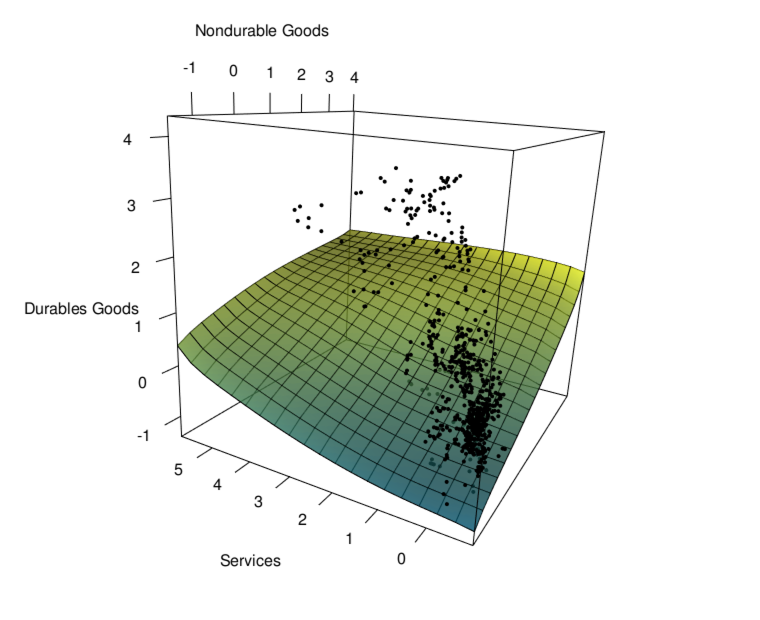
(a) Quantile surface, confidence level $p=0.05$

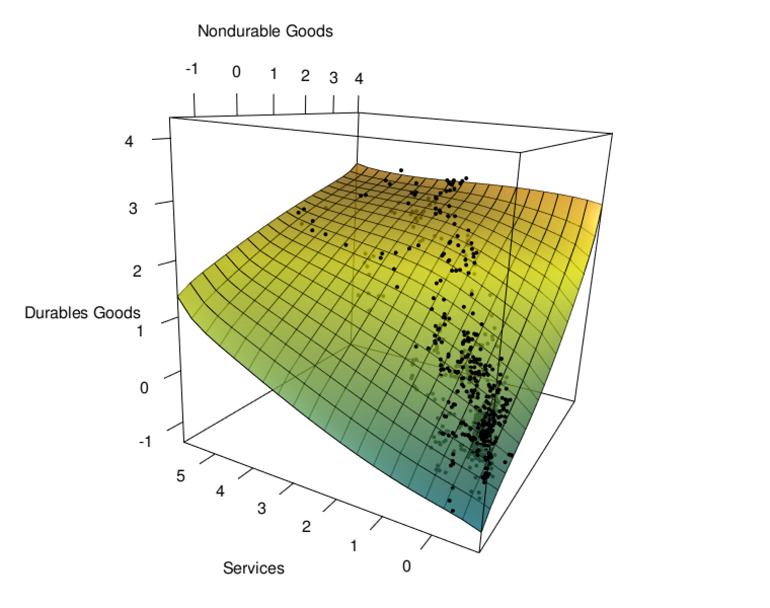
(b) Quantile surface, confidence level $p=0.5$

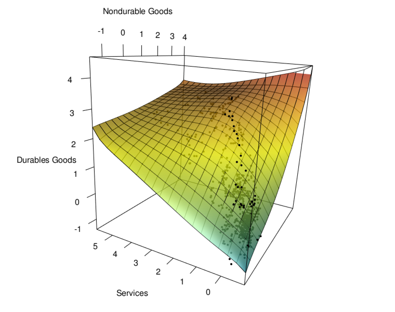
(c) Quantile surface, confidence level $p=0.95$

Figure 1: Quantile surfaces of confidence levels $0.05,0.5,0.95$ in the experiments in Section 9.1. The black dots are the data points.

9.2 Dimensionality Reduction by Reduced Rank Tensor for Factor Model of Mixture CVaRs

The second numerical experiment examines the reduced rank method (Section 7) for the Factor Model of Mixture CVaRs (Section 8). We illustrate that the low-rank representation of parameter tensor is efficient to compute by showing the in-sample error curves. The full data set described in Section 9.1 is used in the calibration.

Model

Consider the Factor Model of Mixture CVaRs in tensor format

$$G(p,\bm{x},\bm{a})=\bm{A}\cdot\left(\bar{\bm{Q}}(p)\otimes\bigotimes_{k=1}^{\emph{K}}\bm{B}_{k}(x_{k})\right)\;,$$ (40)

where $\bar{\bm{Q}}(p)$ is the vector of basis CVaR functions. We use $I$-spline basis of degree three with five knots and CVaR function of exponential distribution as basis CVaR functions. for splines $\bm{B}_{k}(x_{k})$, we still use B-spline of degree three with six knots.

Calibration

The experiment considers cases where the rank, R in (31), equals 1, 3, and 10. For each case, 21 optimization steps are conducted using the alternating algorithm. The error function for the regression is defined by replacing $\bm{\mathcal{E}}_{p}$ in Problem 4.2 with the error defined in (36). Since CVaR is often used to measure tail risk, we choose more tail confidence levels in the optimization. The confidence levels are $0.25,0.55,0.60,0.65,\cdots,0.95$. No penalty is applied to the smoothness of splines as in Section 9.1, since the aim is to compare the models with varying ranks. Note that the low-rank representation alone does not guarantee improvements in out-of-sample test, since the smoothness condition is unconstrained and may lead to overfit. The combination of the low-rank representation with P-spline is left for future study.

Results

The objective values at each step are displayed in Figure 2. A higher rank corresponds to a smaller final objective value and a greater number of steps to converge. Nonetheless, the optimization converges in a few steps for all three cases, demonstrating the efficiency of the algorithm for estimation.

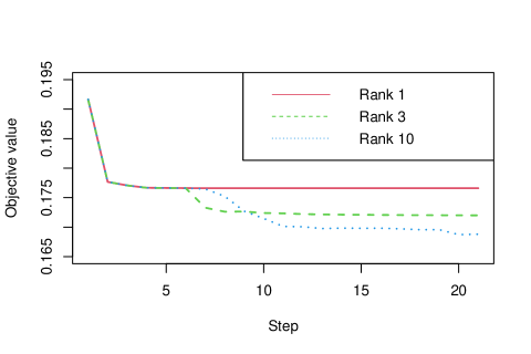
Figure 2: Stepwise objective value of alternating algorithm of rank $1$, $3$ and $10$ of experiments in Section 9.2.

References

- de Boor and Daniel (1974) C. de Boor and James W. Daniel. Splines with nonnegative -spline coefficients. Mathematics of Computation, 28(126):565–568, 1974. ISSN 00255718, 10886842. URL http://www.jstor.org/stable/2005928.
- Quandt (1972) Richard E. Quandt. A new approach to estimating switching regressions. Journal of the American Statistical Association, 67(338):306–310, 1972. ISSN 01621459. URL http://www.jstor.org/stable/2284373.
- Koenker and Bassett (1978) Roger Koenker and Gilbert Bassett. Regression quantiles. Econometrica, 46(1):33–50, 1978. ISSN 00129682, 14680262. URL http://www.jstor.org/stable/1913643.
- Koenker and Hallock (2001) Roger Koenker and Kevin F. Hallock. Quantile regression. Journal of Economic Perspectives, 15(4):143–156, December 2001. doi: 10.1257/jep.15.4.143. URL https://www.aeaweb.org/articles?id=10.1257/jep.15.4.143.
- Hitchcock (1927) Frank L. Hitchcock. The expression of a tensor or a polyadic as a sum of products. Journal of Mathematics and Physics, 6(1-4):164–189, 1927. doi: https://doi.org/10.1002/sapm192761164. URL https://onlinelibrary.wiley.com/doi/abs/10.1002/sapm192761164.
- Harshman (1970) Richard A. Harshman. Foundations of the parafac procedure: Models and conditions for an ”explanatory” multi-model factor analysis. 1970.
- Carroll and Chang (1970) J. Douglas Carroll and Jih Jie Chang. Analysis of individual differences in multidimensional scaling via an n-way generalization of “eckart-young” decomposition. Psychometrika, 35:283–319, 1970.
- Rockafellar and Uryasev (2000) R. Tyrrell Rockafellar and Stanislav Uryasev. Optimization of Conditional Value-at-Risk. Journal of Risk, 2:21–41, 2000.
- Rockafellar and Uryasev (2002) R. Tyrrell Rockafellar and Stanislav Uryasev. Conditional Value-at-Risk for general loss distributions. Journal of Banking and Finance, pages 1443–1471, 2002.
- Newey and Powell (1987) Whitney K. Newey and James L. Powell. Asymmetric least squares estimation and testing. Econometrica, 55(4):819–847, 1987. ISSN 00129682, 14680262. URL http://www.jstor.org/stable/1911031.
- Rockafellar and Uryasev (2013) R. Tyrrell Rockafellar and Stan Uryasev. The fundamental risk quadrangle in Risk Management, Optimization and Statistical Estimation. Surveys in Operations Research and Management Science 18, 2013.
- Papp (2011) Dávid Papp. Optimization models for shape-constrained function estimation problems involving nonnegative polynomials and their restrictions. 2011.
- Papp and Alizadeh (2014) Dávid Papp and Farid Alizadeh. Shape-constrained estimation using nonnegative splines. Journal of Computational and Graphical Statistics, 23(1):211–231, 2014. doi: 10.1080/10618600.2012.707343. URL https://doi.org/10.1080/10618600.2012.707343.
- Hersbach (2000) Hans Hersbach. Decomposition of the continuous ranked probability score for ensemble prediction systems. Weather and Forecasting, 15(5):559 – 570, 2000. doi: 10.1175/1520-0434(2000)015¡0559:DOTCRP¿2.0.CO;2. URL https://journals.ametsoc.org/view/journals/wefo/15/5/1520-0434_2000_015_0559_dotcrp_2_0_co_2.xml.
- Sillitto (1969) G. P. Sillitto. Derivation of approximants to the inverse distribution function of a continuous univariate population from the order statistics of a sample. Biometrika, 56(3):641–650, 1969. ISSN 00063444. URL http://www.jstor.org/stable/2334672.
- Karvanen (2006) Juha Karvanen. Estimation of quantile mixtures via l-moments and trimmed l-moments. Computational Statistics & Data Analysis, 51(2):947–959, 2006. ISSN 0167-9473. doi: https://doi.org/10.1016/j.csda.2005.09.014. URL https://www.sciencedirect.com/science/article/pii/S0167947305002513.
- Keelin (2016) Thomas W. Keelin. The metalog distributions. Decision Analysis, 13(4):243–277, 2016. doi: 10.1287/deca.2016.0338. URL https://doi.org/10.1287/deca.2016.0338.
- Peng et al. (2022) Cheng Peng, Yizhou Li, and Stan Uryasev. Mixture quantiles calibrated with constrained linear regression. 2022.
- DeSarbo and Cron (1988) Wayne S DeSarbo and William L Cron. A maximum likelihood methodology for clusterwise linear regression. Journal of classification, 5(2):249–282, 1988.
- Ghahramani et al. (1996) Zoubin Ghahramani, Geoffrey E Hinton, et al. The em algorithm for mixtures of factor analyzers. Technical report, Technical Report CRG-TR-96-1, University of Toronto, 1996.
- Villani et al. (2009) Mattias Villani, Robert Kohn, and Paolo Giordani. Regression density estimation using smooth adaptive gaussian mixtures. Journal of Econometrics, 153(2):155–173, 2009. ISSN 0304-4076. doi: https://doi.org/10.1016/j.jeconom.2009.05.004. URL https://www.sciencedirect.com/science/article/pii/S0304407609001419.
- Yuksel et al. (2012) Seniha Esen Yuksel, Joseph N. Wilson, and Paul D. Gader. Twenty years of mixture of experts. IEEE Transactions on Neural Networks and Learning Systems, 23(8):1177–1193, 2012. doi: 10.1109/TNNLS.2012.2200299.
- Koenker et al. (1994) Roger Koenker, Pin Ng, and Stephen Portnoy. Quantile smoothing splines. Biometrika, 81(4):673–680, 1994.
- He et al. (1998) X. He, P. Ng, and S. Portnoy. Bivariate quantile smoothing splines. Journal of the Royal Statistical Society: Series B (Statistical Methodology), 60(3):537–550, 1998.
- Koenker (2011) Roger Koenker. Additive models for quantile regression: Model selection and confidence bandaids. Brazilian Journal of Probability and Statistics, 25(3):239 – 262, 2011. doi: 10.1214/10-BJPS131. URL https://doi.org/10.1214/10-BJPS131.
- Bondell et al. (2010) Howard D Bondell, Brian J Reich, and Huixia Wang. Noncrossing quantile regression curve estimation. Biometrika, 97(4):825–838, 2010.
- Chernozhukov et al. (2010) Victor Chernozhukov, Iván Fernández-Val, and Alfred Galichon. Quantile and probability curves without crossing. Econometrica, 78(3):1093–1125, 2010. doi: https://doi.org/10.3982/ECTA7880. URL https://onlinelibrary.wiley.com/doi/abs/10.3982/ECTA7880.
- Koenker (1984) Roger Koenker. A note on l-estimates for linear models. Statistics & Probability Letters, 2(6):323–325, 1984. ISSN 0167-7152. doi: https://doi.org/10.1016/0167-7152(84)90040-3. URL https://www.sciencedirect.com/science/article/pii/0167715284900403.
- Zou and Yuan (2008) Hui Zou and Ming Yuan. Composite quantile regression and the oracle model selection theory. The Annals of Statistics, 36(3):1108 – 1126, 2008. doi: 10.1214/07-AOS507. URL https://doi.org/10.1214/07-AOS507.
- Sottile and Frumento (2022) Gianluca Sottile and Paolo Frumento. Robust estimation and regression with parametric quantile functions. Computational Statistics & Data Analysis, 171:107471, 2022. ISSN 0167-9473. doi: https://doi.org/10.1016/j.csda.2022.107471. URL https://www.sciencedirect.com/science/article/pii/S0167947322000512.
- Angrist et al. (2006) Joshua Angrist, Victor Chernozhukov, and Iván Fernández-Val. Quantile regression under misspecification, with an application to the u.s. wage structure. Econometrica, 74(2):539–563, 2006.
- Reich et al. (2011) Brian J. Reich, Montserrat Fuentes, and David B. Dunson. Bayesian spatial quantile regression. Journal of the American Statistical Association, 106(493):6–20, 2011. doi: 10.1198/jasa.2010.ap09237. URL https://doi.org/10.1198/jasa.2010.ap09237. PMID: 23459794.
- Lian et al. (2015) Heng Lian, Jie Meng, and Zengyan Fan. Simultaneous estimation of linear conditional quantiles with penalized splines. Journal of Multivariate Analysis, 141:1–21, 2015. ISSN 0047-259X. doi: https://doi.org/10.1016/j.jmva.2015.06.010. URL https://www.sciencedirect.com/science/article/pii/S0047259X15001554.
- Frumento and Bottai (2016) Paolo Frumento and Matteo Bottai. Parametric modeling of quantile regression coefficient functions. Biometrics, 72(1):74–84, 2016. doi: https://doi.org/10.1111/biom.12410. URL https://onlinelibrary.wiley.com/doi/abs/10.1111/biom.12410.
- Yuan et al. (2017) Yuan Yuan, Nan Chen, and Shiyu Zhou. Modeling regression quantile process using monotone b-splines. Technometrics, 59(3):338–350, 2017. doi: 10.1080/00401706.2016.1211553. URL https://doi.org/10.1080/00401706.2016.1211553.
- Matheson and Winkler (1976) James E. Matheson and Robert L. Winkler. Scoring rules for continuous probability distributions. Management Science, 22(10):1087–1096, 1976. doi: 10.1287/mnsc.22.10.1087. URL https://doi.org/10.1287/mnsc.22.10.1087.
- Laio and Tamea (2006) Francesco Laio and Stefania Tamea. Verification tools for probabilistic forecasts of continuous hydrological variables. Hydrology and Earth System Sciences, 11:1267–1277, 2006.
- Hothorn et al. (2014) Torsten Hothorn, Thomas Kneib, and Peter Bühlmann. Conditional transformation models. Journal of the Royal Statistical Society. Series B (Statistical Methodology), 76(1):3–27, 2014. ISSN 13697412, 14679868. URL http://www.jstor.org/stable/24772743.
- Gouttes et al. (2021) Adèle Gouttes, Kashif Rasul, Mateusz Koren, Johannes Stephan, and Tofigh Naghibi. Probabilistic time series forecasting with implicit quantile networks, 2021. URL https://arxiv.org/abs/2107.03743.
- Berrisch and Ziel (2021) Jonathan Berrisch and Florian Ziel. Crps learning. Journal of Econometrics, 2021. ISSN 0304-4076. doi: https://doi.org/10.1016/j.jeconom.2021.11.008. URL https://www.sciencedirect.com/science/article/pii/S0304407621002724.
- Zhang et al. (2022) Qian Zhang, Anuran Makur, and Kamyar Azizzadenesheli. Functional linear regression of cdfs, 2022. URL https://arxiv.org/abs/2205.14545.
- Fakoor et al. (2021) Rasool Fakoor, Taesup Kim, Jonas Mueller, Alexander J. Smola, and Ryan J. Tibshirani. Flexible model aggregation for quantile regression, 2021. URL https://arxiv.org/abs/2103.00083.
- Chernozhukov and Umantsev (2001) Victor Chernozhukov and Len Umantsev. Conditional value-at-risk: Aspects of modeling and estimation. Empirical Economics, 26(1):271–292, 2001.
- Gasthaus et al. (2019) Jan Gasthaus, Konstantinos Benidis, Yuyang Wang, Syama Sundar Rangapuram, David Salinas, Valentin Flunkert, and Tim Januschowski. Probabilistic forecasting with spline quantile function rnns. In Kamalika Chaudhuri and Masashi Sugiyama, editors, Proceedings of the Twenty-Second International Conference on Artificial Intelligence and Statistics, volume 89 of Proceedings of Machine Learning Research, pages 1901–1910. PMLR, 16–18 Apr 2019. URL https://proceedings.mlr.press/v89/gasthaus19a.html.
- Bremnes (2020) John Bjørnar Bremnes. Ensemble postprocessing using quantile function regression based on neural networks and bernstein polynomials. Monthly Weather Review, 148(1):403 – 414, 2020. doi: 10.1175/MWR-D-19-0227.1. URL https://journals.ametsoc.org/view/journals/mwre/148/1/mwr-d-19-0227.1.xml.
- Rigby and Stasinopoulos (2005) R. A. Rigby and D. M. Stasinopoulos. Generalized additive models for location, scale and shape,(with discussion). Applied Statistics, 54:507–554, 2005.
- Pan et al. (2016) Maodong Pan, Weihua Tong, and Falai Chen. Compact implicit surface reconstruction via low-rank tensor approximation. Computer-Aided Design, 78:158–167, 2016. ISSN 0010-4485. doi: https://doi.org/10.1016/j.cad.2016.05.007. URL https://www.sciencedirect.com/science/article/pii/S0010448516300276. SPM 2016.
- Kolda and Bader (2009) Tamara G. Kolda and Brett W. Bader. Tensor decompositions and applications. SIAM Review, 51(3):455–500, 2009. doi: 10.1137/07070111X. URL https://doi.org/10.1137/07070111X.
- Rabanser et al. (2017) Stephan Rabanser, Oleksandr Shchur, and Stephan Günnemann. Introduction to tensor decompositions and their applications in machine learning, 2017. URL https://arxiv.org/abs/1711.10781.
- Lian et al. (2019) Heng Lian, Weihua Zhao, and Yanyuan Ma. Multiple quantile modeling via reduced-rank regression. Statistica Sinica, 29(3):1439–1464, 2019. ISSN 10170405, 19968507. URL https://www.jstor.org/stable/26706009.
- Chen et al. (2021) Liang Chen, Juan J. Dolado, and Jesús Gonzalo. Quantile factor models. Econometrica, 89(2):875–910, 2021. doi: https://doi.org/10.3982/ECTA15746. URL https://onlinelibrary.wiley.com/doi/abs/10.3982/ECTA15746.
- Rockafellar and Royset (2013) R. Tyrrell Rockafellar and Johannes O. Royset. Superquantiles and Their Applications to Risk, Random Variables, and Regression, chapter Chapter 8, pages 151–167. 2013. doi: 10.1287/educ.2013.0111. URL https://pubsonline.informs.org/doi/abs/10.1287/educ.2013.0111.
- Rockafellar et al. (2014) R.T. Rockafellar, J.O. Royset, and S.I. Miranda. Superquantile regression with applications to buffered reliability, uncertainty quantification, and conditional value-at-risk. European Journal of Operational Research, 234(1):140–154, 2014. ISSN 0377-2217. doi: https://doi.org/10.1016/j.ejor.2013.10.046. URL https://www.sciencedirect.com/science/article/pii/S0377221713008692.
- Golodnikov et al. (2019) Alex Golodnikov, Viktor Kuzmenko, and Stan Uryasev. Cvar regression based on the relation between cvar and mixed-quantile quadrangles. Journal of Risk and Financial Management, 12(3), 2019. ISSN 1911-8074. doi: 10.3390/jrfm12030107. URL https://www.mdpi.com/1911-8074/12/3/107.
- Rockafellar and Royset (2018) R Tyrrell Rockafellar and Johannes O Royset. Superquantile/cvar risk measures: Second-order theory. Annals of Operations Research, 262(1):3–28, 2018.
- Kuzmenko (2020) VM Kuzmenko. A new family of expectiles and its properties. Cybernetics and Computer Technologies, 2020.
- Eilers and Marx (1996) Paul H. C. Eilers and Brian D. Marx. Flexible smoothing with B-splines and penalties. Statistical Science, 11(2):89 – 121, 1996. doi: 10.1214/ss/1038425655. URL https://doi.org/10.1214/ss/1038425655.
- Eilers and Marx (2003) Paul H.C. Eilers and Brian D. Marx. Multivariate calibration with temperature interaction using two-dimensional penalized signal regression. Chemometrics and Intelligent Laboratory Systems, 66(2):159–174, 2003. ISSN 0169-7439. doi: https://doi.org/10.1016/S0169-7439(03)00029-7. URL https://www.sciencedirect.com/science/article/pii/S0169743903000297.
- Ramsay (1988) J. O. Ramsay. Monotone regression splines in action. Statistical Science, 3(4):425–441, 1988. ISSN 08834237. URL http://www.jstor.org/stable/2245395.
- Curry and Schoenberg (1988) H. B. Curry and I. J. Schoenberg. On Pólya Frequency Functions IV: The Fundamental Spline Functions and their Limits, pages 347–383. Birkhäuser Boston, Boston, MA, 1988. ISBN 978-1-4899-0433-1. doi: 10.1007/978-1-4899-0433-1˙17. URL https://doi.org/10.1007/978-1-4899-0433-1_17.
- Engle (1982) Robert F. Engle. Autoregressive conditional heteroscedasticity with estimates of the variance of united kingdom inflation. Econometrica, 50(4):987–1007, 1982. ISSN 00129682, 14680262. URL http://www.jstor.org/stable/1912773.
- Gourieroux and Jasiak (2008) C. Gourieroux and J. Jasiak. Dynamic quantile models. Journal of Econometrics, 147(1):198–205, 2008. ISSN 0304-4076. doi: https://doi.org/10.1016/j.jeconom.2008.09.028. URL https://www.sciencedirect.com/science/article/pii/S0304407608001358. Econometric modelling in finance and risk management: An overview.
- Koenker (2005) Roger Koenker. Quantile Regression. Econometric Society Monographs. Cambridge University Press, 2005. doi: 10.1017/CBO9780511754098.
- Portnoy (1991) Stephen Portnoy. Asymptotic behavior of the number of regression quantile breakpoints. SIAM Journal on Scientific and Statistical Computing, 12(4):867–883, 1991. doi: 10.1137/0912047. URL https://doi.org/10.1137/0912047.
- Newey and McFadden (1994) Whitney K. Newey and Daniel McFadden. Chapter 36 large sample estimation and hypothesis testing. volume 4 of Handbook of Econometrics, pages 2111–2245. Elsevier, 1994. doi: https://doi.org/10.1016/S1573-4412(05)80005-4. URL https://www.sciencedirect.com/science/article/pii/S1573441205800054.
- Norton et al. (2021) Matthew Norton, Valentyn Khokhlov, and Stan Uryasev. Calculating cvar and bpoe for common probability distributions with application to portfolio optimization and density estimation. Annals of Operations Research, 299(1):1281–1315, 2021.
- McCracken and Ng (2016) Michael W McCracken and Serena Ng. Fred-md: A monthly database for macroeconomic research. Journal of Business & Economic Statistics, 34(4):574–589, 2016.
- (68) Christian Zimmermann. Astonishingly different inflation across goods categories. URL https://fredblog.stlouisfed.org/2022/11/astonishingly-different-inflation-across-goods-categories/. Accessed: 2023-03-14.
- Zabarankin et al. (2016) Michael Zabarankin, Stan Uryasev, et al. Statistical decision problems. Springer, 2016.
- Benaglia et al. (2009) Tatiana Benaglia, Didier Chauveau, David R. Hunter, and Derek S. Young. mixtools: An r package for analyzing mixture models. Journal of Statistical Software, 32(6):1–29, 2009. doi: 10.18637/jss.v032.i06. URL https://www.jstatsoft.org/index.php/jss/article/view/v032i06.
- Azzalini and Capitanio (2003) Adelchi Azzalini and Antonella Capitanio. Distributions generated by perturbation of symmetry with emphasis on a multivariate skew t-distribution. Journal of the Royal Statistical Society: Series B (Statistical Methodology), 65(2):367–389, 2003. doi: https://doi.org/10.1111/1467-9868.00391. URL https://rss.onlinelibrary.wiley.com/doi/abs/10.1111/1467-9868.00391.