Image Shortcut Squeezing:
Countering Perturbative Availability Poisons with Compression

Zhuoran Liu Zhengyu Zhao Martha Larson

Abstract

Perturbative availability poisons (PAPs) add small changes to images to prevent their use for model training. Current research adopts the belief that practical and effective approaches to countering PAPs do not exist. In this paper, we argue that it is time to abandon this belief. We present extensive experiments showing that 12 state-of-the-art PAP methods are vulnerable to Image Shortcut Squeezing (ISS), which is based on simple compression. For example, on average, ISS restores the CIFAR-10 model accuracy to $81.73\%$ , surpassing the previous best preprocessing-based countermeasures by $37.97\%$ absolute. ISS also (slightly) outperforms adversarial training and has higher generalizability to unseen perturbation norms and also higher efficiency. Our investigation reveals that the property of PAP perturbations depends on the type of surrogate model used for poison generation, and it explains why a specific ISS compression yields the best performance for a specific type of PAP perturbation. We further test stronger, adaptive poisoning, and show it falls short of being an ideal defense against ISS. Overall, our results demonstrate the importance of considering various (simple) countermeasures to ensure the meaningfulness of analysis carried out during the development of PAP methods. Our code is available at https://github.com/liuzrcc/ImageShortcutSqueezing.

Availability Poisoning, Unlearnable Examples, Data Poisoning, Shortcut Learning

Refer to caption — Figure 1: An illustration of our Image Shortcut Squeezing (ISS) for countering perturbative availability poisons (PAPs). The model accuracy is reduced by PAPs but is then restored by our ISS. Results are reported for EM (Huang et al., 2021) poisons on CIFAR-10.

1 Introduction

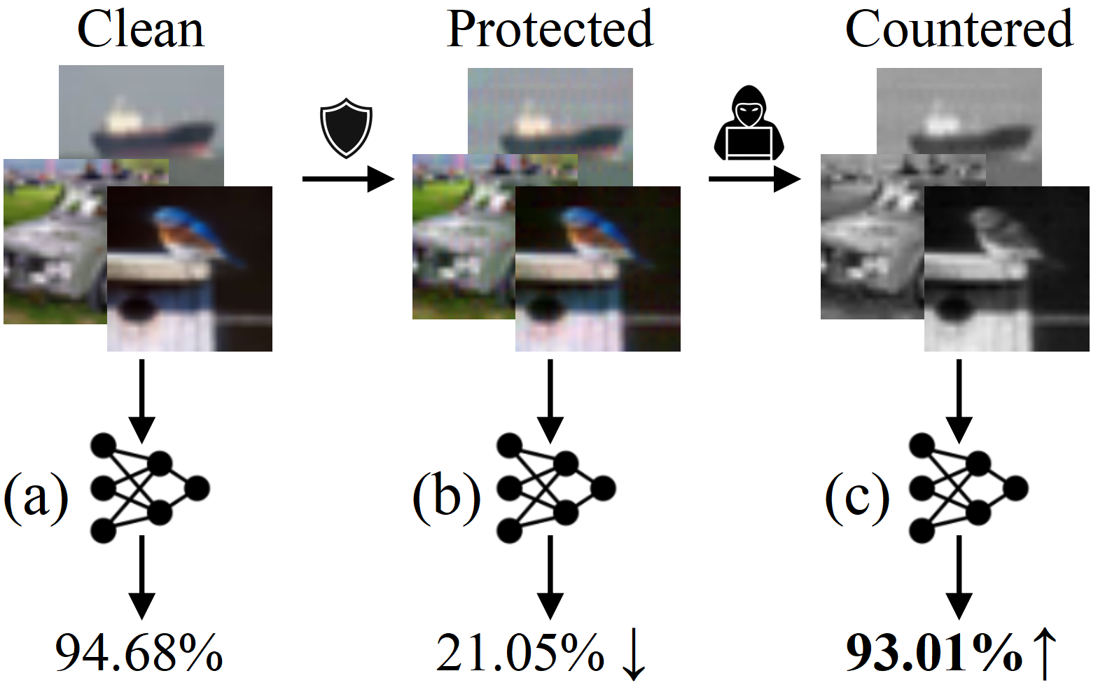
The ever-growing amount of data that is easily available online has driven the tremendous advances of deep neural networks (DNNs) (Schmidhuber, 2015; LeCun et al., 2015; He et al., 2016; Brown et al., 2020). However, online data may be proprietary or contain private information, raising concerns about unauthorized use. Perturbative availability poisons (PAPs) are recognized as a promising approach to data protection and recently a large number of PAP methods have been proposed that add perturbations to images which block training by acting as shortcuts (Shen et al., 2019; Huang et al., 2021; Fowl et al., 2021b, a). As illustrated by Figure 1 (a) $\rightarrow$ (b), the high test accuracy of a DNN model is substantially reduced by PAPs.

Existing research has shown that PAPs can be compromised to a limited extent by preprocessing-based-countermeasures, such as data augmentations (Huang et al., 2021; Fowl et al., 2021b) and pre-filtering (Fowl et al., 2021b; Chen et al., 2023). However, a widely adopted belief is that no approaches exist that are capable of effectively countering PAPs. Adversarial training (AT) has been proven to be a strong countermeasure (Tao et al., 2021; Wen et al., 2023). However, it is not considered to be a practical one, since it requires a large amount of computation and also gives rise to a non-negligible trade-off in test accuracy of the clean (non-poisoned) model (Madry et al., 2018; Zhang et al., 2019). Further, AT trained with a specific $L_{p}$ norm is hard to generalize to other norms (Tramer & Boneh, 2019; Laidlaw et al., 2021).

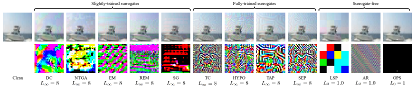
In this paper, we challenge the belief that it is impossible to counter PAP methods both easily and effectively by demonstrating that they are vulnerable to simple compression. First, we categorize 12 PAP methods into three categories with respect to the surrogate models they use during poison generation: slightly-trained (Feng et al., 2019; Huang et al., 2021; Yuan & Wu, 2021; Fu et al., 2021; van Vlijmen et al., 2022), fully-trained (Shen et al., 2019; Tao et al., 2021; Fowl et al., 2021b; Chen et al., 2023), and surrogate-free (Wu et al., 2023; Yu et al., 2022; Sandoval-Segura et al., 2022). Then, we analyze perturbations/shortcuts that are learned with these methods and demonstrate that they are strongly dependent on features that are learned in different training stages of the model. Specifically, we find that the methods using a slightly-trained surrogate model prefer low-frequency shortcuts, while those using a fully-trained model prefer high-frequency shortcuts.

Building on this new understanding, we propose Image Shortcut Squeezing (ISS), a simple, compression-based approach to countering PAPs. As illustrated by Figure 1 (b) $\rightarrow$ (c), the low test accuracy of the poisoned DNN model is restored by our ISS to be close to the original accuracy. In particular, grayscale compression is used to eliminate low-frequency shortcuts, and JPEG compression is used to eliminate high-frequency shortcuts. We also show that our understanding of high vs. low frequency can also help eliminate surrogate-free PAPs (Wu et al., 2023; Yu et al., 2022; Sandoval-Segura et al., 2022). Our ISS substantially outperforms previously studied data augmentation and pre-filtering countermeasures. ISS also achieves comparable results to adversarial training and has three main advantages: 1) generalizability to multiple $L_{p}$ norms, 2) efficiency, and 3) low trade-off in clean model accuracy (see Section 4.2 for details).

We further test the performance of ISS against potentially stronger PAP methods that are aware of ISS and can be adapted to it. We show that they are not ideal against our ISS. Overall, we hope our study can inspire more meaningful analyses of PAP methods and encourage future research to evaluate various (simple) countermeasures when developing new PAP methods.

In sum, we make the following main contributions:

•

We identify the strong dependency of the perturbation frequency patterns on the nature of the surrogate model. Based on this new insight, we show that 12 existing perturbative availability poison (PAP) methods are indeed very vulnerable to simple image compression.
•

We propose Image Shortcut Squeezing (ISS), a simple yet effective approach to countering PAPs. ISS applies image compression operations, such as JPEG and grayscale, to poisoned images for restoring the model accuracy.
•

We demonstrate that ISS outperforms existing data augmentation and pre-filtering countermeasures by a large margin and is comparable to adversarial training but is more generalizable to multiple $L_{p}$ norms and more efficient.
•

We explore stronger, adaptive poisons against our ISS and provide interesting insights into understanding PAPs, e.g., about the model learning preference of different perturbations.

2 Related Work

2.1 Perturbative Availability Poison (PAP)

Perturbative availability poison (PAP) has been extensively studied. TensorClog (TC) (Shen et al., 2019) optimizes the poisons by exploiting the parameters of a pre-trained surrogate to cause the gradient to vanish. Deep Confuse (DC) (Feng et al., 2019) collects the training trajectories of a surrogate classifier for learning a poison generator, which is computationally intensive. Error-Minimizing (EM) poisons (Huang et al., 2021) minimizes the classification errors of images on a surrogate classifier with respect to their original labels in order to make them “unlearnable examples”. The surrogate is also alternatively updated to mimic the model training dynamics during poison generation. Hypocritical (HYPO) (Tao et al., 2021) follows a similar idea to EM but uses a pre-trained surrogate rather than the above bi-level optimization. Targeted Adversarial Poisoning (TAP) (Fowl et al., 2021b) also exploits a pre-trained model but minimizes classification errors of images with respect to incorrect target labels rather than original labels.

Robust Error-Minimizing (REM) (Fu et al., 2021) improves the poisoning effects against adversarial training (with a relatively small norm) by replacing the normally-trained surrogate in EM with an adversarially-trained model. Similar approaches (Wang et al., 2021; Wen et al., 2023) on poisoning against adversarial training are also proposed. The usability of poisoning is also validated in scenarios requiring transferability (Ren et al., 2023) or involving unsupervised learning (He et al., 2023; Zhang et al., 2023).

There are also studies focusing on revising the surrogate, e.g., Self-Ensemble Protection (Chen et al., 2023), which aggregates multiple training model checkpoints, and NTGA (Yuan & Wu, 2021), which adopts the generalized neural tangent kernel to model the surrogate as Gaussian Processes (Jacot et al., 2018). ShortcutGen (SG) (van Vlijmen et al., 2022) learns a poison generator based on a randomly initialized fixed surrogate and shows its efficiency compared to the earlier generative method, Deep Confuse.

Different from all the above methods, recent studies also explore surrogate-free PAPs (Evtimov et al., 2021; Yu et al., 2022; Sandoval-Segura et al., 2022). Intuitively, simple patterns, such as random noise (Huang et al., 2021) and semantics (e.g., MNIST-like digits) (Evtimov et al., 2021), can be used as learning shortcuts when they form different distributions for different classes. Very recent studies also synthesize more complex, linear separable patterns to boost the poisoning performance based on sampling from a high dimensional Gaussian distribution (Yu et al., 2022) and further refining it by introducing the autoregressive process (Sandoval-Segura et al., 2022). One Pixel Shortcut (OPS) specifically explores the model vulnerability to sparse poisons and shows that perturbing only one pixel is sufficient to generate strong poisons (Wu et al., 2023).

In the domain of facial recognition, PAP methods, e.g., Fawkes (Shan et al., 2020) and LowKey (Cherepanova et al., 2021), have also been studied. However, their protection algorithms closely resemble the PAPs as discussed above. Specifically, Fawkes adopts a feature-layer loss similar to SEP and a robust surrogate model similar to REM, to boost transferability. LowKey adopts ensemble surrogate models similar to SEP and a pre-processing step similar to TAP, to boost transferability and imperceptibility.

In this paper, we evaluate our ISS against 12 representative PAP methods as presented above. In particular, we consider poisons constrained by different $L_{p}$ norms. Because of their technical similarity to two of the 12 approaches, we do not consider Fawkes and LowKey in our evaluation.

2.2 PAP Countermeasures

As mentioned in Section 1, existing research has mainly relied on adversarial training (AT) for countering PAPs (Tao et al., 2021; Wen et al., 2023). However, AT is not practical due to the requirement of large computations and the non-negligible trade-off in test accuracy of the clean model (Madry et al., 2018; Zhang et al., 2019). In addition, image preprocessing, e.g., data augmentations (Huang et al., 2021; Fowl et al., 2021b) and pre-filtering (Fowl et al., 2021b; Chen et al., 2023), also show substantial effects but not comparable to AT. In the domain of face recognition, countermeasures are also discussed but either require stronger assumptions or lack a concrete algorithm (Radiya-Dixit et al., 2022). See more discussions in Appendix D.

In this paper, we compare our ISS against existing countermeasures and particularly highlight its generalizability to unknown norms (Tramer & Boneh, 2019; Laidlaw et al., 2021) and simplicity.

2.3 Adversarial Perturbations and Countermeasures

Simple image compressions, such as JPEG, bit depth reduction, and smoothing, are effective for countering adversarial perturbations based on the assumption that they are inherently high-frequency noise (Dziugaite et al., 2016; Das et al., 2017; Xu et al., 2017). Other image transformations commonly used for data augmentations, e.g., resizing, rotating, and shifting, are also shown to be effective (Xie et al., 2018; Tian et al., 2018; Dong et al., 2019). However, such image pre-processing operations may be bypassed when the attacker is aware of them and then adapted to them (Carlini et al., 2019). Differently, adversarial training (AT) is effective against adaptive attacks and is considered to be the most powerful defense so far (Tramer et al., 2020).

Besides (training-time) data poisons, adversarial perturbations can also be used for data protection, but at inference time. Related research has explored person-related recognition (Oh et al., 2016, 2017; Sattar et al., 2020; Rajabi et al., 2021) and social media mining (Larson et al., 2018; Li et al., 2019; Liu et al., 2020). An overview of inference-time data protection in images is provided by (Orekondy et al., 2017).

Our ISS is based on compression. We specifically evaluate its compression effects in Section 4.5.

3 Analysis of Perturbative Availability Poisons

3.1 Problem Formulation

We formulate the problem of countering perturbative availability poisons (PAPs) in the context of image classification. There are two parties involved, the data protector and exploiter. The data protector poisons their own images to prevent them from being used by the exploiter for training a well-generalizable classifier. Specifically, here the poisoning is achieved by adding imperceptible perturbations. The data exploiter is aware that their collected images may contain poisons and so apply countermeasures to ensure their trained classifier is still well-generalizable. The success of the countermeasure is measured by the accuracy of the classifier on clean test images, and the higher, the more successful.

Formally stated, the protector aims to make a classifier $F$ generalize poorly on the clean image distribution $\mathcal{D}$ , from which the clean training set $\mathcal{S}$ is sampled:

\displaystyle\max_{\boldsymbol{\delta}}\,\,\mathbb{E}_{(\boldsymbol{x},y)\sim\mathcal{D}}\bigg{[}\mathcal{L}\left(F(\boldsymbol{x};\boldsymbol{\theta}^{\prime}({\boldsymbol{\delta}})),y\right)\bigg{]}

(1)

\displaystyle\text{s.t.}\,\,\boldsymbol{\theta}^{\prime}({\boldsymbol{\delta}})=\operatorname*{argmin}_{\boldsymbol{\theta}({\boldsymbol{\delta}})}\sum_{(\boldsymbol{x}_{i},y_{i})\in\mathcal{S}}\mathcal{L}(F(\boldsymbol{x}_{i}+\boldsymbol{\delta}_{i};\boldsymbol{\theta}({\boldsymbol{\delta}}),y_{i}),

(2)

where $\boldsymbol{\theta}({\boldsymbol{\delta}})$ represents the parameters of the poisoned classifier, $F$ , where $\boldsymbol{\delta}$ denotes the additive perturbations with $\epsilon$ as the $L_{p}$ bound. $\mathcal{L}(\cdot;\cdot)$ is the cross-entropy loss, which takes as input a pair of model output $F(\boldsymbol{x}_{i};\boldsymbol{\theta})$ and the corresponding label $y_{i}$ .

The exploiter aims to counter the poisons by applying a countermeasure $C$ to restore the model accuracy even when it is trained on poisoned data $\mathcal{P}$ :

\displaystyle\min_{\boldsymbol{\theta}}\sum_{(\boldsymbol{x}_{i},y_{i})\in\mathcal{P}}\mathcal{L}(F(C(\boldsymbol{x}_{i}+\boldsymbol{\delta}_{i});\boldsymbol{\theta}),y_{i}).

(3)

3.2 Categorization of Existing PAP Methods

We carried out an extensive survey of existing PAP methods, which allowed us to identify three categories of them regarding the type of their used surrogate classifiers. These three categories are: Generating poisons 1) with a slightly-trained surrogate, 2) with a fully-trained surrogate, and 3) in a surrogate-free manner. Table 1 provides an overview of this categorization. In the first category, the surrogate is at its early training stage. Existing methods in this category either fixes (Yuan & Wu, 2021; van Vlijmen et al., 2022) or alternatively updates (Feng et al., 2019; Huang et al., 2021; Fu et al., 2021) the surrogate during optimizing the poisons. In the second category, the surrogate has been fully trained. Existing methods in this category fix the surrogate (Shen et al., 2019; Tao et al., 2021; Fowl et al., 2021b; Chen et al., 2023) but in principle, it may also be possible that the model is alternatively updated. In the third category, no surrogate is used but the poisons are synthesized by sampling from Gaussian distributions (Yu et al., 2022; Sandoval-Segura et al., 2022) or optimized with a perceptual loss (Wu et al., 2023).

Table 1: Categorization of existing PAP methods.

PAP Methods	Surrogate Model
DC (Feng et al., 2019)	Slightly-Trained
NTGA (Yuan & Wu, 2021)
EM (Huang et al., 2021)
REM (Fu et al., 2021)
SG (van Vlijmen et al., 2022)
TC (Shen et al., 2019)	Fully-Trained
HYPO (Tao et al., 2021)
TAP (Fowl et al., 2021b)
SEP (Chen et al., 2023)
LSP (Yu et al., 2022)	Surrogate-Free
AR (Sandoval-Segura et al., 2022)
OPS (Wu et al., 2023)

3.3 Frequency-based Interpretation of Perturbations

Poisoned CIFAR-10 images and their corresponding perturbations for the 12 methods are visualized in Figure 2. As can be seen, the four methods that adopt a fully-trained surrogate tend to generate perturbations in patterns having a high spatial frequency. This is consistent with the common finding in the adversarial example literature that adversarial perturbations are normally high-frequency (Guo et al., 2019). In contrast, the five methods that adopt a slight-trained surrogate exhibit spatially low-frequency patterns but large differences across color channels.

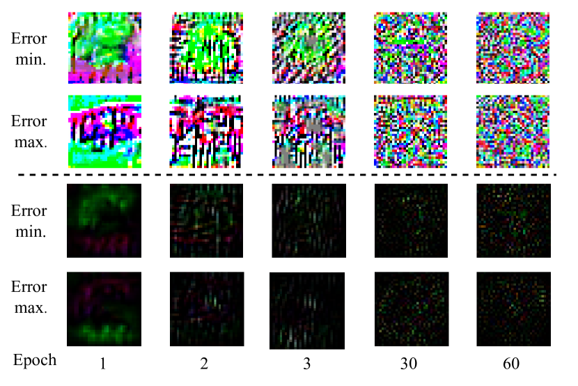
We hypothesize that the above phenomenon can be explained by the frequency principle (Rahaman et al., 2019; Xu et al., 2019; Luo et al., 2021), that is, deep neural networks often fit target functions from low to high frequencies during training. Accordingly, the poisons optimized against a slightly-trained model capture low-frequency patterns while those optimized against a fully-trained model capture high-frequency patterns (Rahaman et al., 2019; Xu et al., 2019; Luo et al., 2021). In order to validate this hypothesis, we further try optimizing poisons using either the error-minimizing or error-maximizing loss against the surrogate at its various training epochs. We visualize the resulting poisoned images and their corresponding perturbations in Figure 3. As can be been, the spatial frequency of the perturbations gets increasingly higher as the surrogate goes to a later training epoch.

Different from those surrogate-based methods, the three surrogate-free methods have full control of the perturbation patterns they aim to synthesize. However, we notice that they still follow our frequency-based interpretation of perturbation patterns. Specifically, the perturbations of LSP (Yu et al., 2022) are uniformly upsampled from a Gaussian distribution and so exhibit patch-based low-frequency patterns. On the other hand, the perturbations of AR (Sandoval-Segura et al., 2022) are generally based on sliding convolutions over the image and so exhibit texture-based high-frequency patterns. OPS (Wu et al., 2023) perturbations only contain one pixel and so can be treated as an extreme case of high-frequency patterns.

3.4 Our Image Shortcut Squeezing

Based on the above new frequency-based interpretation, we propose Image Shortcut Squeezing (ISS), a simple, image compression-based countermeasure against PAPs. We rely on different compression operations suitable for eliminating different types of perturbations. Overall, a specific compression operation is applied to the $C(\cdot)$ in Eq. 3.

For perturbations with low frequency but large differences across color channels, we use grayscale transformation to suppress such color differences. We expect grayscale transformation to not sacrifice too much the test accuracy of a clean model because color information is known to contribute little to the DNNs’ performance in differentiating objects (Xie & Richmond, 2018). For perturbations with high frequency, we follow existing research on eliminating adversarial perturbations to use common image compression operations, such as JPEG and bit depth reduction (BDR) (Dziugaite et al., 2016; Das et al., 2017; Xu et al., 2017). We expect grayscale transformation to not sacrifice too much the test accuracy of a clean model because DNNs are known to be resilient to small amounts of image compression, e.g., JPEG with a higher quality factor than 10 (Dodge & Karam, 2016).

4 Experiments

In this section, we evaluate our Image Shortcut Squeezing (ISS) and other countermeasures against 12 representative PAP methods. We focus our experiments on the basic setting in which the surrogate (if it is used) and target models are the same and the whole training set is poisoned. We also explore more challenging poisoning scenarios with unseen target models or partial poisoning (poisoning a randomly selected proportion or a specific class).

4.1 Experimental Settings

Datasets and models. We consider three datasets: CIFAR-10 (Krizhevsky, 2009), CIFAR-100 (Krizhevsky, 2009), and a 100-class subset of ImageNet (Deng et al., 2009). If not mentioned specifically, on CIFAR-10 and CIFAR-100, we use 50000 images for training and 10000 images for testing. For the ImageNet subset, we select 20% images from the first 100 classes of the official ImageNet training set for training and all corresponding images in the official validation set for testing. If not mentioned specifically, ResNet-18 (RN-18) (He et al., 2016) is used as the surrogate model and target model. To study transferability, we consider target models with diverse architectures: ResNet-34 (He et al., 2016), VGG-19 (Simonyan & Zisserman, 2015), DenseNet-121 (Huang et al., 2017), MobileNet-V2 (Sandler et al., 2018), and ViT (Dosovitskiy et al., 2021).

Training and poisoning settings. We train the CIFAR-10/100 models for 60 epochs and the ImageNet models for 100 epochs. We use SGD with a momentum of 0.9, a learning rate of 0.025, and cosine weight decay. We adopt the torchvision transforms module for implementing Grayscale, JPEG, and bit depth reduction (BDR) in our Image Shortcut Squeezing (ISS). We consider 12 representative existing poisoning methods as listed in Table 1 under various $L_{p}$ norm bounds. A brief description of 12 methods can be found in Appendix A. Specifically, we follow existing work and use $L_{\infty}=8$ , $L_{2}=1.0$ , and $L_{0}=1$ .

Table 2: Clean test accuracy (%) of models trained on CIFAR-10 poisons and with our Image Shortcut Squeezing (Gray and JPEG) vs. other countermeasures. Note that TC is known to not work well under small norms, e.g., our

L_{\infty}=8

(Fowl et al., 2021b). Hyperparameters for different countermeasures can be found in Appendix B.

Norm	Poisons/Countermeasures	w/o	Cutout	CutMix	Mixup	Gaussian	Mean	Median	BDR	Gray	JPEG	Gray+JPEG	AT
Norm	Clean (no poison)	94.68	95.10	95.50	95.01	94.17	45.32	85.94	88.65	92.41	85.38	83.79	84.99
$L_{\infty}=8$	DC (Feng et al., 2019)	16.30	15.14	17.99	19.39	17.21	19.57	15.82	61.10	93.07	81.84	83.09	78.00
	NTGA (Yuan & Wu, 2021)	42.46	42.07	27.16	43.03	42.84	37.49	42.91	62.50	74.32	69.49	69.86	70.05
	EM (Huang et al., 2021)	21.05	20.63	26.19	32.83	12.41	20.60	21.70	36.46	93.01	81.50	83.06	84.80
	REM (Fu et al., 2021)	25.44	26.54	29.02	34.48	27.44	25.35	31.57	40.77	92.84	82.28	83.00	82.99
	SG (van Vlijmen et al., 2022)	33.05	24.12	29.46	39.66	31.92	46.87	49.53	70.14	86.42	79.49	79.21	76.38
	TC (Shen et al., 2019)	88.70	86.70	88.43	88.19	82.58	72.25	84.27	84.85	79.75	85.29	82.43	84.55
	HYPO (Tao et al., 2021)	71.54	70.60	67.54	72.54	72.46	40.27	65.53	83.50	61.86	85.45	82.94	84.91
	TAP (Fowl et al., 2021b)	8.17	10.04	10.73	19.14	9.26	21.82	32.75	45.99	9.11	83.87	81.94	83.31
	SEP (Chen et al., 2023)	3.85	4.47	9.41	15.59	3.96	14.43	35.65	47.43	3.57	84.37	82.18	84.12
$L_{2}=1.0$	LSP (Yu et al., 2022)	19.07	19.87	20.89	26.99	19.25	28.85	29.85	66.19	82.47	83.01	79.05	84.59
$L_{2}=1.0$	AR (Sandoval-Segura et al., 2022)	13.28	12.07	12.39	13.25	15.45	45.15	70.96	31.54	34.04	85.15	82.81	83.17
$L_{0}=1$	OPS (Wu et al., 2023)	36.55	67.94	76.40	45.06	19.29	23.50	85.16	53.76	42.44	82.53	79.10	14.41

4.2 Evaluation in the Common Scenario

We first evaluate our ISS against 12 representative poisoning methods in the common scenario where the surrogate and target models are the same and the whole training dataset is poisoned. Experimental results on CIFAR-10 shown in Table 2 demonstrate that ISS can substantially restore the clean test accuracy of poisoned models in all cases. Consistent with our new insight in Section 3.3, grayscale yields the best performance in countering methods that rely on low-frequency perturbations with large color differences (see more results by other color compression methods on EM in Appendix C). In contrast, JPEG and BDR are the best against methods that rely on high-frequency perturbations. Additional results for other hyperparameters of JPEG and BDR in Table 13 of Appendix B show that milder settings yield worse results. In addition, we can also apply ISS without determining the specific poisons by directly using Gray+JPEG. The results demonstrate that this combination is globally effective against all 12 PAP methods, with only a small decrease in clean model accuracy.

Our ISS also outperforms other countermeasures. Specifically, data augmentations applied to clean models increase test accuracy but they are not effective against poisons. Image Smoothing is sometimes effective, e.g., median filtering performs the best against OPS as expected since it is effective against impulsive noise. Adversarial training (AT) achieves comparable performance to our ISS for $L_{\infty}$ and $L_{2}$ norms but much worse performance for the $L_{0}$ norm. This verifies the higher generalizability of our ISS to unseen norms. It is worth noting that the ISS training time is only $\frac{1}{7}$ of the AT training time on CIFAR-10. The efficiency of our ISS becomes more critical when the dataset is larger and the image resolution is higher. Additional experimental results for $L_{\infty}=16$ shown in Table 3 confirm the general effectiveness of our ISS.

We further conduct experiments on CIFAR-100 and ImageNet. Note that for CIFAR-100, we only test the PAP methods that include CIFAR-100 experiments in their original work. For ImageNet, the poison optimization process is very time-consuming, especially for NTGA (Yuan & Wu, 2021) and Deep Confuse (Feng et al., 2019). Therefore, following the original work, these two methods are tested with only two classes. Note that such time-consuming PAP methods are not good candidates for data protection in practice. Experimental results on CIFAR-100 and ImageNet shown in Table 4 and Table 5 confirm the general effectiveness of our ISS.

Table 3: Additional results on CIFAR-10 with larger perturbation norms:

L_{2}=2.0

for LSP and

L_{\infty}=16

for the rest.

Poisons	w/o	Cutout	CutMix	Mixup	Gray	JPEG	AT
Clean	94.68	95.10	95.50	95.01	92.41	88.65	84.99
EM	16.33	14.0	13.41	20.22	60.85	63.44	61.58
REM	24.89	25.0	22.85	29.51	42.85	76.59	80.14
HYPO	58.3	54.22	48.26	57.27	45.38	85.07	84.90
TAP	10.98	10.96	9.46	17.97	6.94	84.19	83.35
SEP	3.84	8.90	15.79	9.27	5.70	84.35	84.07
LSP	19.07	19.87	20.89	26.99	82.47	83.01	84.59

Table 4: Additional results on CIFAR-100.

Poisons	w/o	Cutout	CutMix	Mixup	Gray	JPEG
Clean	77.44	76.72	80.50	78.56	71.79	57.79
EM	7.25	6.70	7.03	10.68	67.46	56.01
REM	9.37	12.46	10.40	15.05	57.27	55.77
TC	57.52	60.56	59.19	59.77	47.93	58.94
TAP	9.00	10.30	8.73	19.16	8.84	83.77
SEP	3.21	3.21	3.98	7.49	2.10	58.18
LSP	3.06	4.43	6.12	5.61	44.62	53.49
AR	3.01	2.85	3.49	2.19	24.99	57.87
OPS	23.78	57.98	56.03	22.71	32.62	54.92

Table 5: Additional results on ImageNet subset. Following their original papers, NTGA and DC are tested with only two classes.

Poisons	w/o	Cutout	CutMix	Mixup	Gray	JPEG
Clean	62.04	61.14	65.100	64.32	58.24	58.20
EM	31.52	30.42	42.98	21.44	49.78	49.88
REM	11.12	11.62	12.50	17.62	44.70	18.16
TAP	24.64	23.00	18.72	28.62	24.30	44.74
LSP	26.32	27.64	17.22	2.5	31.42	30.78
NTGA	70.79	63.42	70.53	68.42	83.42	76.58
DC	65.00	-	-	-	85.00	74.00

4.3 Evaluation in Challenging Scenarios

Partial poisoning. In practical scenarios, it is common that only a proportion of the training data can be poisoned. Therefore, we follow existing work (Fowl et al., 2021b; Huang et al., 2020) to test such partial poisoning settings. We poison a certain proportion of the training data and mix it with the rest clean data for training the target model.

Specifically, we test two partial poisoning settings: first, randomly selecting a certain proportion of the images, and, second, selecting a specific class. In the first setting, as shown in Table 6, the poisons are effective only when a very large proportion of the training data is poisoned. For example, on average, even when 80% of data are poisoned, the model accuracy is only reduced by about 10 %. In the second setting, we choose to poison all training samples from class automobile on CIFAR-10. Table 7 demonstrates that almost all poisoning methods are very effective in the full poisoning setting. In both settings, our ISS is effective against all PAP methods.

Table 6: Clean test accuracy (%) of CIFAR-10 target models under different poisoning proportions. TC is tested with

L_{\infty}=26

Poisons	ISS	0.1	0.2	0.4	0.6	0.8	0.9
DC	w/o	94.29	94.26	93.20	91.66	87.19	80.14
	Gray	92.73	92.57	92.37	91.51	90.49	89.50
	JPEG	84.89	85.26	84.43	83.61	83.02	82.69
EM	w/o	94.37	93.63	92.62	91.07	86.63	79.57
	Gray	92.60	92.62	92.52	92.23	90.96	89.69
	JPEG	84.61	84.79	84.96	84.86	84.93	84.40
REM	w/o	94.39	94.56	94.37	94.43	94.19	81.39
	Gray	92.63	92.81	92.78	92.82	92.73	86.62
	JPEG	84.64	85.53	84.82	85.37	85.38	82.44
SG	w/o	94.47	94.40	93.46	91.21	87.75	83.40
	Gray	92.81	92.65	91.90	90.65	88.44	85.26
	JPEG	84.94	84.61	84.11	82.66	80.76	79.38
TC	w/o	93.81	94.09	93.70	93.59	93.02	91.47
	Gray	91.98	92.38	92.03	91.96	91.03	87.71
	JPEG	85.24	85.01	85.23	85.28	85.23	84.37
HYPO	w/o	93.94	94.43	93.34	92.56	90.64	89.35
	Gray	92.59	92.39	91.37	90.06	88.03	86.37
	JPEG	85.61	85.18	85.39	85.21	85.25	85.10
TAP	w/o	94.09	93.94	92.75	91.27	88.42	85.98
	Gray	92.62	91.94	90.73	89.26	85.93	83.18
	JPEG	85.24	84.42	84.86	84.98	84.51	84.36
SEP	w/o	94.12	93.45	92.76	91.22	87.82	85.01
	Gray	92.57	92.04	91.09	89.25	86.31	82.95
	JPEG	85.27	85.27	85.25	84.71	84.07	84.80
LSP	w/o	94.69	94.42	92.81	91.38	88.07	82.26
	Gray	93.12	92.56	92.67	92.20	90.78	89.65
	JPEG	85.01	84.58	84.88	83.49	83.27	81.67
AR	w/o	94.66	94.38	93.82	91.80	88.42	82.36
	Gray	92.85	92.69	92.53	91.24	89.88	85.35
	JPEG	85.37	84.75	85.35	85.35	85.07	87.27
OPS	w/o	94.47	94.11	92.61	91.49	87.19	82.65
	Gray	92.65	92.27	91.36	89.34	85.24	81.37
	JPEG	84.75	84.88	84.55	83.98	82.87	81.33

Table 7: Partial poisoning for class automobile on CIFAR-10. TC is tested with

L_{\infty}=26

Poisons	w/o	Gray	JPEG	BDR
DC	1.60	69.00	88.30	52.20
NTGA	51.70	94.20	90.40	75.30
EM	0.10	48.60	94.30	9.60
REM	0.80	34.40	90.40	2.50
SG	27.75	88.39	78.59	70.05
TC	0.50	0.20	92.50	37.20
HYPO	4.00	3.00	94.90	56.80
TAP	0.00	0.10	93.90	38.10
SEP	0.00	0.00	94.70	15.50
LSP	67.30	86.90	95.10	83.20
AR	97.70	97.60	94.60	95.10
OPS	28.90	28.50	93.60	72.10

Table 8: Clean test accuracy (%) of CIFAR-10 target models in the transfer setting. Note that AR, LSP, and OPS are surrogate-free. Four CNN models (ResNet-34, VGG-19, DenseNet-121, and MobileNet-V2) and one ViT are considered as the target model. TensorClog (TC) is tested with

L_{\infty}=26

Poisons	ISS	R34	V19	D121	M2	ViT
DC	w/o	18.06	16.59	16.05	17.81	24.09
	Gray	83.13	80.32	83.93	78.78	44.83
	JPEG	82.64	80.34	83.38	80.30	53.35
NTGA	w/o	40.19	47.13	16.67	40.75	31.82
	Gray	71.84	76.89	64.07	62.28	58.25
	JPEG	67.00	72.17	73.76	70.18	53.00
EM	w/o	29.96	34.70	30.61	30.10	18.84
	Gray	86.97	87.03	84.84	82.81	63.28
	JPEG	84.21	82.46	84.86	82.20	56.33
REM	w/o	25.88	29.04	28.31	24.08	32.22
	Gray	75.20	77.99	70.53	66.21	63.00
	JPEG	82.35	80.70	81.74	80.01	56.13
SG	w/o	29.64	48.5	28.88	30.75	18.11
	Gray	86.53	87.12	86.07	81.34	42.22
	JPEG	79.57	77.78	79.77	75.87	56.27
TC	w/o	87.71	85.47	78.04	78.51	69.86
	Gray	78.48	75.14	66.72	62.39	61.86
	JPEG	84.56	82.66	83.95	82.60	55.51
HYPO	w/o	80.64	81.59	81.48	78.27	67.49
	Gray	75.25	76.65	74.29	69.81	53.02
	JPEG	85.55	83.39	85.03	83.95	55.17
TAP	w/o	7.89	8.59	8.64	10.02	41.32
	Gray	9.38	11.51	8.77	8.29	42.49
	JPEG	84.42	81.95	84.28	82.24	57.35
SEP	w/o	3.11	6.70	4.41	5.29	25.56
	Gray	4.00	5.40	4.20	4.70	22.23
	JPEG	84.64	83.38	84.55	83.25	56.94
LSP	w/o	15.98	17.39	19.79	17.32	26.65
	Gray	71.10	82.11	73.06	70.61	53.36
	JPEG	79.57	78.72	79.66	76.79	60.41
AR	w/o	21.31	19.78	13.54	16.08	22.91
	Gray	70.54	76.92	67.35	62.01	53.22
	JPEG	85.62	83.95	85.46	83.50	54.88
OPS	w/o	37.06	36.3	40.03	27.35	30.25
	Gray	44.29	42.21	38.32	38.71	21.77
	JPEG	82.84	80.70	82.83	80.42	62.93

Transferability to unseen models. In realistic scenarios, the protector may not know the details of the target model. In this case, the transferability of the poisons is desirable. Table 8 demonstrates that all PAP methods achieve high transferability to diverse model architectures and our ISS is effective against all of them. It is also worth noting that there is no clear correlation between the transferability and the similarity between the surrogate and target models. For example, transferring from ResNet-18 to ViT is not always harder than to other CNN models.

4.4 Adaptive Poisons to ISS

In the adversarial example literature, image compression operations can be bypassed when the attacker is adapted to them (Shin & Song, 2017; Carlini et al., 2019). Similarly, we evaluate strong adaptive poisons against our ISS using two PAP methods, EM ( $L_{\infty}$ ) and LSP ( $L_{2}$ ). We assume that the protector can be adapted to grayscale and/or JPEG in our ISS. Specifically, for EM, we add a differentiable JPEG compression module (Shin & Song, 2017) and/or a differentiable grayscale module into its bi-level poison optimization process. For LSP, we increase the patch size to 16 $\times$ 16 to decrease high-frequency features so that JPEG will be less effective, and we make sure the pixel values are the same for three channels to bypass grayscale.

Table 9 demonstrates that for EM, the adaptive grayscale poisons are effective against grayscale, but adaptive JPEG-10 noises are not effective against JPEG. As hinted by (Shin & Song, 2017), using an ensemble of JPEG with different quality factors might be necessary for better adaptive poisoning. We also implement BPDA (Athalye et al., 2018a) with the same JPEG quality factor (i.e., JPEG-10) and find that our ISS still ensures a very high model accuracy, i.e., 83.70 %. For LSP, we observe that even though adaptive LSP is more effective against the combination of JPEG and grayscale than the other two individual compressions, it is insufficient to serve as a good adaptive protector. On the other hand, adaptive LSP also fails against the model without ISS, indicating that the additional operations (grayscale and larger patches) largely constrain its poisoning effects.

Given that the protector may have full knowledge of our ISS, we believe that better-designed adaptive poisons can bypass our ISS in the future.

Table 9: Clean test accuracy (%) of four different target models under EM poisoning and its adaptive variants on CIFAR-10. Results are reported for

L_{\infty}=8

and Table 14 in Appendix reports results of EM for

L_{\infty}=16

, which follow the same pattern.

Poisons	w/o	Gray	JPEG	G&J	Ave.
EM	21.05	93.01	81.50	83.06	69.66
EM-Gray	17.81	16.60	76.71	74.16	46.32
EM-JPEG	17.11	89.18	83.11	82.85	68.06
EM-G&J	48.93	46.29	69.48	66.26	57.74
LSP	19.07	82.47	83.01	79.05	65.90
LSP-G&J	93.01	90.34	84.38	82.13	87.47

4.5 Further Analyses

Working Mechanism of ISS. Here we illustrate the working mechanism of our ISS by ensuring that the poisons are the exact factor that is used by the poisoned model for prediction. To this end, we follow (Fowl et al., 2021b) to use poisoned images to both train and test the model. In this case, if the test accuracy (on poisoned images) is high, it demonstrates that the perturbations in the poisoned images are actually learned by the model. In addition, we also train and test the model on poisoned images but differently, the testing (poisoned) images are pre-processed using our ISS. In this case, if the test accuracy (on poisoned images) decreases, it demonstrates that ISS can suppress the perturbations at inference time. The results in Table 10 validate our hypotheses.

Table 10: Test accuracy (%) on clean, poisoned, and ISS-preprocessed poisoned test sets of models that are trained on different poisons.

Test/ Poisons	DC	NTGA	EM	REM	SG	TC	HYPO	TAP	SEP	LSP	AR	OPS
Clean	17.96	-	16.77	26.04	37.50	87.86	73.06	11.63	4.91	15.29	16.37	17.50
Poisoned	97.20	97.85	99.85	99.97	96.72	93.79	99.98	100.0	99.99	100.0	99.94	99.83
Poisoned+ISS	11.17	24.86	11.89	20.68	25.39	24.16	16.68	11.33	10.13	10.06	13.83	12.61

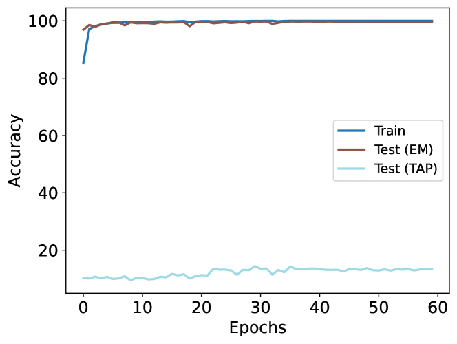
Relative Model Preference of different poisons. We explore the relative model preference of low-frequency vs. high-frequency poisons. This scenario is practically interesting because the same online data might be poisoned by different methods. Inspired by the experiments on the model preference of MNIST vs. CIFAR data in (Shah et al., 2020), we simply add up the EM and TAP perturbations for each image. The perturbation norm is doubled accordingly. For example, for perturbations with $L_{\infty}=8$ , the composite perturbations range from $-16$ to $16$ . We train a model (using the original image labels) on the composite perturbations of EM and TAP and test it on either EM or TAP perturbations.

As shown in Figure 4, the model converges fast and reaches a high test accuracy on EM but not on the TAP. It indicates that TAP perturbations are less preferred than EM perturbations by the model during training.

ISS for a combination of different types of poisons. We create poisons by combining the two well-known low-frequency and high-frequency methods, i.e., EM and TAP. Specifically, we take the average of the perturbations of these two methods. As shown in Table 11, our ISS is still effective against this combination.

Table 11: Clean test accuracy (%) of models trained on CIFAR-10 poisons that is a combination of low-frequency poison EM and high-frequency TAP.

Poisons/ISS	w/o	Gray	JPEG
EM	21.05	93.01	81.50
TAP	8.17	9.11	83.87
EM+TAP	36.07	18.93	84.62

ISS for both training and testing. Our ISS only applies to the training data for removing the poisons. However, in this case, it may cause a possible distribution shift between the training and test data. Here we explore such a shift by comparing ISS with another variant that applies compression to both the training and test data. Table 12 demonstrates that in most cases, these two versions of ISS do not lead to substantial differences.

Table 12: Clean test accuracy (%) for ISS (Gray and JPEG), which applies compression only to training data or to both training and test data (denoted with suffix-TT).

Poisons	Gray-TT	Gray	JPEG-TT	JPEG
Clean	92.62	92.41	79.56	85.38
DC	83.79	93.07	79.41	81.84
NTGA	65.42	74.32	62.84	69.49
EM	90.75	93.01	78.96	81.50
REM	73.38	92.84	79.39	82.28
SG	88.26	86.42	72.96	79.49
TC	76.41	75.88	79.42	83.69
HYPO	75.20	61.86	79.63	85.60
TAP	9.53	9.11	78.65	83.87
SEP	2.93	3.57	79.28	84.37
LSP	76.23	75.77	68.73	78.69
AR	68.95	69.37	79.26	85.38
OPS	46.53	42.44	76.87	82.53

5 Conclusion and Outlook

In this paper, we challenge the common belief that there are no practical and effective countermeasures to perturbative availability poisons (PAPs). Specifically, we show that 12 state-of-the-art PAP methods can be substantially countered by Image Shortcut Squeezing (ISS), which is based on simple compression. ISS outperforms other previously studied countermeasures, such as data augmentations and adversarial training. Our in-depth investigation leads to a new insight that the property of PAP perturbations depends on the type of surrogate model used during poison generation. We also show the ineffectiveness of adaptive poisons to ISS. We hope that further studies could consider various (simple) countermeasures during the development of new PAP methods.

For future work, on the countermeasure side, we would further improve ISS on the trade-off between its effectiveness and the decrease of clean model accuracy by exploring other (simple) accuracy-preserving operations. In addition, to achieve a countermeasure that is more effective against unknown poisons, it would be promising to explore more advanced combination strategies of operations or conduct automatic attack identification and then apply attack-specific operations. On the protection side, we encourage future work to develop effective (adaptive) protection methods against our ISS and other potential countermeasures.

Acknowledgements

We are grateful to Alex Kolmus, Dirren van Vlijmen, Rui Wen, Tijn Berns, Tom Heskes, Twan van Laarhoven, and the anonymous reviewers for discussion and feedback on this work. We thank Shutong Wu, Jie Ren, and Hao He for providing source codes. Part of this work was carried out on the Dutch national e-infrastructure with the support of SURF Cooperative.

References

Athalye et al. (2018a) Athalye, A., Carlini, N., and Wagner, D. Obfuscated gradients give a false sense of security: Circumventing defenses to adversarial examples. In ICML, 2018a.
Athalye et al. (2018b) Athalye, A., Engstrom, L., Ilyas, A., and Kwok, K. Synthesizing robust adversarial examples. In ICML, 2018b.
Brown et al. (2020) Brown, T., Mann, B., Ryder, N., Subbiah, M., Kaplan, J. D., Dhariwal, P., Neelakantan, A., Shyam, P., Sastry, G., Askell, A., et al. Language models are few-shot learners. In NeurIPS, 2020.
Carlini et al. (2019) Carlini, N., Athalye, A., Papernot, N., Brendel, W., Rauber, J., Tsipras, D., Goodfellow, I., Madry, A., and Kurakin, A. On evaluating adversarial robustness. arXiv:1902.06705, 2019.
Chen et al. (2023) Chen, S., Yuan, G., Cheng, X., Gong, Y., Qin, M., Wang, Y., and Huang, X. Self-ensemble protection: Training checkpoints are good data protectors. In ICLR, 2023.
Cherepanova et al. (2021) Cherepanova, V., Goldblum, M., Foley, H., Duan, S., Dickerson, J., Taylor, G., and Goldstein, T. Lowkey: Leveraging adversarial attacks to protect social media users from facial recognition. In ICLR, 2021.
Das et al. (2017) Das, N., Shanbhogue, M., Chen, S.-T., Hohman, F., Chen, L., Kounavis, M. E., and Chau, D. H. Keeping the bad guys out: Protecting and vaccinating deep learning with jpeg compression. arXiv:1705.02900, 2017.
Deng et al. (2009) Deng, J., Dong, W., Socher, R., Li, L.-J., Li, K., and Fei-Fei, L. Imagenet: A large-scale hierarchical image database. In CVPR, pp. 248–255, 2009.
Dodge & Karam (2016) Dodge, S. and Karam, L. Understanding how image quality affects deep neural networks. In QoMEX, 2016.
Dong et al. (2019) Dong, Y., Pang, T., Su, H., and Zhu, J. Evading defenses to transferable adversarial examples by translation-invariant attacks. In CVPR, 2019.
Dosovitskiy et al. (2021) Dosovitskiy, A., Beyer, L., Kolesnikov, A., Weissenborn, D., Zhai, X., Unterthiner, T., Dehghani, M., Minderer, M., Heigold, G., Gelly, S., et al. An image is worth 16x16 words: Transformers for image recognition at scale. In ICLR, 2021.
Dziugaite et al. (2016) Dziugaite, G. K., Ghahramani, Z., and Roy, D. M. A study of the effect of jpg compression on adversarial images. arXiv:1608.00853, 2016.
Evtimov et al. (2021) Evtimov, I., Covert, I., Kusupati, A., and Kohno, T. Disrupting model training with adversarial shortcuts. In ICML Workshop AML, 2021.
Feng et al. (2019) Feng, J., Cai, Q.-Z., and Zhou, Z.-H. Learning to confuse: generating training time adversarial data with auto-encoder. In NeurIPS, 2019.
Fowl et al. (2021a) Fowl, L., Chiang, P.-y., Goldblum, M., Geiping, J., Bansal, A., Czaja, W., and Goldstein, T. Preventing unauthorized use of proprietary data: Poisoning for secure dataset release. arXiv:2103.02683, 2021a.
Fowl et al. (2021b) Fowl, L., Goldblum, M., Chiang, P.-y., Geiping, J., Czaja, W., and Goldstein, T. Adversarial examples make strong poisons. In NeurIPS, 2021b.
Fu et al. (2021) Fu, S., He, F., Liu, Y., Shen, L., and Tao, D. Robust unlearnable examples: Protecting data privacy against adversarial learning. In ICLR, 2021.
Guo et al. (2019) Guo, C., Frank, J. S., and Weinberger, K. Q. Low frequency adversarial perturbation. In UAI, 2019.
He et al. (2023) He, H., Zha, K., and Katabi, D. Indiscriminate poisoning attacks on unsupervised contrastive learning. In ICLR, 2023.
He et al. (2016) He, K., Zhang, X., Ren, S., and Sun, J. Deep residual learning for image recognition. In CVPR, 2016.
Huang et al. (2017) Huang, G., Liu, Z., Van Der Maaten, L., and Weinberger, K. Q. Densely connected convolutional networks. In CVPR, 2017.
Huang et al. (2021) Huang, H., Ma, X., Erfani, S. M., Bailey, J., and Wang, Y. Unlearnable examples: Making personal data unexploitable. In ICLR, 2021.
Huang et al. (2020) Huang, W. R., Geiping, J., Fowl, L., Taylor, G., and Goldstein, T. MetaPoison: Practical general-purpose clean-label data poisoning. In NeurIPS, 2020.
Jacot et al. (2018) Jacot, A., Gabriel, F., and Hongler, C. Neural tangent kernel: Convergence and generalization in neural networks. In NeurIPS, 2018.
Jaderberg et al. (2015) Jaderberg, M., Simonyan, K., Zisserman, A., et al. Spatial transformer networks. In NeurIPS, 2015.
Krizhevsky (2009) Krizhevsky, A. Learning multiple layers of features from tiny images. Technical report, University of Toronto, 2009.
Laidlaw et al. (2021) Laidlaw, C., Singla, S., and Feizi, S. Perceptual adversarial robustness: Defense against unseen threat models. In ICLR, 2021.
Larson et al. (2018) Larson, M., Liu, Z., Brugman, S., and Zhao, Z. Pixel privacy. increasing image appeal while blocking automatic inference of sensitive scene information. In MediaEval, 2018.
LeCun et al. (2015) LeCun, Y., Bengio, Y., and Hinton, G. Deep learning. Nature, 521(7553):436–444, 2015.
Li et al. (2019) Li, C. Y., Shamsabadi, A. S., Sanchez-Matilla, R., Mazzon, R., and Cavallaro, A. Scene privacy protection. In ICASSP, 2019.
Liu et al. (2020) Liu, Z., Zhao, Z., Larson, M., and Amsaleg, L. Exploring quality camouflage for social images. In MediaEval, 2020.
Luo et al. (2021) Luo, T., Ma, Z., Xu, Z.-Q. J., and Zhang, Y. Theory of the frequency principle for general deep neural networks. CSIAM Trans. Appl. Math., 2021.
Madry et al. (2018) Madry, A., Makelov, A., Schmidt, L., Tsipras, D., and Vladu, A. Towards deep learning models resistant to adversarial attacks. In ICLR, 2018.
Naseer et al. (2019) Naseer, M. M., Khan, S. H., Khan, M. H., Shahbaz Khan, F., and Porikli, F. Cross-domain transferability of adversarial perturbations. In NeurIPS, 2019.
Oh et al. (2016) Oh, S. J., Benenson, R., Fritz, M., and Schiele, B. Faceless person recognition: Privacy implications in social media. In ECCV, 2016.
Oh et al. (2017) Oh, S. J., Fritz, M., and Schiele, B. Adversarial image perturbation for privacy protection a game theory perspective. In ICCV, 2017.
Orekondy et al. (2017) Orekondy, T., Schiele, B., and Fritz, M. Towards a visual privacy advisor: Understanding and predicting privacy risks in images. In ICCV, 2017.
Radiya-Dixit et al. (2022) Radiya-Dixit, E., Hong, S., Carlini, N., and Tramèr, F. Data poisoning won’t save you from facial recognition. In ICLR, 2022.
Rahaman et al. (2019) Rahaman, N., Baratin, A., Arpit, D., Draxler, F., Lin, M., Hamprecht, F., Bengio, Y., and Courville, A. On the spectral bias of neural networks. In ICML, 2019.
Rajabi et al. (2021) Rajabi, A., Bobba, R. B., Rosulek, M., Wright, C., and Feng, W.-c. On the (im) practicality of adversarial perturbation for image privacy. In PETS, 2021.
Ren et al. (2023) Ren, J., Xu, H., Wan, Y., Ma, X., Sun, L., and Tang, J. Transferable unlearnable examples. In ICLR, 2023.
Ronneberger et al. (2015) Ronneberger, O., Fischer, P., and Brox, T. U-net: Convolutional networks for biomedical image segmentation. In MICCAI, 2015.
Sandler et al. (2018) Sandler, M., Howard, A., Zhu, M., Zhmoginov, A., and Chen, L.-C. Mobilenetv2: Inverted residuals and linear bottlenecks. In CVPR, 2018.
Sandoval-Segura et al. (2022) Sandoval-Segura, P., Singla, V., Geiping, J., Goldblum, M., Goldstein, T., and Jacobs, D. W. Autoregressive perturbations for data poisoning. In NeurIPS, 2022.
Sattar et al. (2020) Sattar, H., Krombholz, K., Pons-Moll, G., and Fritz, M. Body shape privacy in images: Understanding privacy and preventing automatic shape extraction. In ECCV, 2020.
Schmidhuber (2015) Schmidhuber, J. Deep learning in neural networks: An overview. Neural Networks, 61:85–117, 2015.
Shah et al. (2020) Shah, H., Tamuly, K., Raghunathan, A., Jain, P., and Netrapalli, P. The pitfalls of simplicity bias in neural networks. In NeurIPSw, 2020.
Shan et al. (2020) Shan, S., Wenger, E., Zhang, J., Li, H., Zheng, H., and Zhao, B. Y. Fawkes: Protecting privacy against unauthorized deep learning models. In USENIX Security, 2020.
Shen et al. (2019) Shen, J., Zhu, X., and Ma, D. TensorClog: An imperceptible poisoning attack on deep neural network applications. IEEE Access, 7:41498–41506, 2019.
Shin & Song (2017) Shin, R. and Song, D. Jpeg-resistant adversarial images. In NeurIPSw, 2017.
Simonyan & Zisserman (2015) Simonyan, K. and Zisserman, A. Very deep convolutional networks for large-scale image recognition. In ICLR, 2015.
Tao et al. (2021) Tao, L., Feng, L., Yi, J., Huang, S.-J., and Chen, S. Better safe than sorry: Preventing delusive adversaries with adversarial training. In NeurIPS, 2021.
Tian et al. (2018) Tian, S., Yang, G., and Cai, Y. Detecting adversarial examples through image transformation. In AAAI, 2018.
Tramer & Boneh (2019) Tramer, F. and Boneh, D. Adversarial training and robustness for multiple perturbations. In NeurIPS, 2019.
Tramer et al. (2020) Tramer, F., Carlini, N., Brendel, W., and Madry, A. On adaptive attacks to adversarial example defenses. In NeurIPS, 2020.
van Vlijmen et al. (2022) van Vlijmen, D., Kolmus, A., Liu, Z., Zhao, Z., and Larson, M. Generative poisoning using random discriminators. In ECCVw, 2022.
Wang et al. (2021) Wang, Z., Wang, Y., and Wang, Y. Fooling adversarial training with inducing noise. arXiv:2111.10130, 2021.
Wen et al. (2023) Wen, R., Zhao, Z., Liu, Z., Backes, M., Wang, T., and Zhang, Y. Is adversarial training really a silver bullet for mitigating data poisoning? In ICLR, 2023.
Wu et al. (2023) Wu, S., Chen, S., Xie, C., and Huang, X. One-pixel shortcut: on the learning preference of deep neural networks. In ICLR, 2023.
Xie et al. (2018) Xie, C., Wang, J., Zhang, Z., Ren, Z., and Yuille, A. Mitigating adversarial effects through randomization. ICLR, 2018.
Xie & Richmond (2018) Xie, Y. and Richmond, D. Pre-training on grayscale imagenet improves medical image classification. In ECCVw, 2018.
Xu et al. (2017) Xu, W., Evans, D., and Qi, Y. Feature squeezing: Detecting adversarial examples in deep neural networks. In NDSS, 2017.
Xu et al. (2019) Xu, Z.-Q. J., Zhang, Y., and Xiao, Y. Training behavior of deep neural network in frequency domain. In ICONIP, 2019.
Yu et al. (2022) Yu, D., Zhang, H., Chen, W., Yin, J., and Liu, T.-Y. Availability attacks create shortcuts. In KDD, 2022.
Yuan & Wu (2021) Yuan, C.-H. and Wu, S.-H. Neural tangent generalization attacks. In ICML, 2021.
Zhang et al. (2019) Zhang, H., Yu, Y., Jiao, J., Xing, E., El Ghaoui, L., and Jordan, M. Theoretically principled trade-off between robustness and accuracy. In ICML, 2019.
Zhang et al. (2023) Zhang, J., Ma, X., Yi, Q., Sang, J., Jiang, Y., Wang, Y., and Xu, C. Unlearnable clusters: Towards label-agnostic unlearnable examples. In CVPR, 2023.

Appendix A Brief Descriptions of Implemented PAP Methods

•

Deep Confuse (DC) (Feng et al., 2019): Perturbations are generated from a U-Net (Ronneberger et al., 2015) on CIFAR-10 and encoder-decoder model on two-class ImageNet. The generators are trained on the output of a pseudo-updated classifier, where the classification model is first trained on clean data and then trained on adversarial data to update the generator. We use the implementation from the official GitHub repository.¹¹1https://github.com/kingfengji/DeepConfuse
•

Neural Tangent Generalization Attacks (NTGA) (Yuan & Wu, 2021) (target model-agnostic): NTGA uses Neural Tangent Kernels to approximate target networks and then leverages the approximation to generate perturbations. We use the poisons provided in the official GitHub repository.²²2https://github.com/lionelmessi6410/ntga
•

Error-Minimizing perturbations (EM) (Huang et al., 2020): Bi-level optimizing error-minimizing perturbations after certain steps of training on perturbed samples that are from the last iteration. The surrogate model is trained on-the-fly with perturbed training samples. We use the implementation from the official GitHub repository.³³3https://github.com/HanxunH/Unlearnable-Examples/
•

Robust Error-Minimizing perturbations (REM) (Fu et al., 2021): Same as EM, but the model is adversarially trained and the perturbations generation is equipped with expectation over transformation technique (EOT) (Athalye et al., 2018b). We use the implementation from the official GitHub repository.⁴⁴4https://github.com/fshp971/robust-unlearnable-examples/
•

Shortcut generator (SG) (van Vlijmen et al., 2022): Perturbations are generated from a ResNet-like encoder-decoder model from (Naseer et al., 2019). Different from another generative poisoning Deep Confuse, the discriminator model is randomly initialized without training. We use the CIFAR-10 poisons (version ‘SG’) provided by the authors by private communication.
•

TensorClog (TC) (Shen et al., 2019): A second-order derivative with respect to training data is calculated to iteratively optimize the perturbations to minimize the gradients of model loss with respect to the weights of model layers. We use the implementation from the official GitHub repository for poisons ( $L_{\infty}=26$ ) on CIFAR-10⁵⁵5https://github.com/JC-S/TensorClog_Public. We also use the implementation from https://github.com/lhfowl/adversarial_poisons for poisons ( $L_{\infty}=8,16$ ) on CIFAR-10.
•

Hypocritical perturbations (HYPO) (Tao et al., 2021): Similar to EM, but the error-minimizing perturbations are generated on a pre-trained surrogate model which is trained on clean data. We use the implementation from the official GitHub repository.⁶⁶6https://github.com/TLMichael/Delusive-Adversary
•

Targeted Adversarial Poisoning (TAP) (Fowl et al., 2021b): Targeted adversarial examples by PGD (Madry et al., 2018) and Spatial Transformer Networks (STN) module (Jaderberg et al., 2015). The poisoning target labels are different from the original labels, but the target labels are the same for poisoning images whose clean versions are from the same class. We use the implementation from the official GitHub repository.⁷⁷7https://github.com/lhfowl/adversarial_poisons
•

Self-Ensemble Protection (SEP) (Chen et al., 2023) SEP ensembles intermediate checkpoints when training on the clean training set to create perturbations. SEP is currently the state-of-the-art protection on CIFAR-10. We use the implementation from the official GitHub repository.⁸⁸8https://github.com/Sizhe-Chen/SEP
•

Linear separable Synthetic Perturbations (LSP) (Yu et al., 2022): Linearly separable Gaussian samples are listed by order and then up-scaled to the size of the image. Perturbations that are sampled from the same Gaussian are added to the same class. We use the implementation from the official GitHub repository.⁹⁹9https://github.com/dayu11/Availability-Attacks-Create-Shortcuts/
•

AutoRegressive poisoning (AR) (Sandoval-Segura et al., 2022) Autoregressive process generates perturbations that CNN favors during training. We use the CIFAR-10 poisons provided by the authors in the official GitHub repository.¹⁰¹⁰10https://github.com/psandovalsegura/autoregressive-poisoning
•

One Pixel Shortcut (OPS) (Wu et al., 2023): OPS generates one pixel shortcut by searching the pixel that creates the most significant mean pixel value change for all images from one class. The perturbations are dataset-dependent. We use the implementation from the official GitHub repository.¹¹¹¹11https://github.com/cychomatica/One-Pixel-Shotcut

Appendix B Hyperparameters for Different Countermeasures

If not explicitly mentioned, we use JPEG with a quality factor of 10 and bit depth reduction (BDR) with 2 bits. For grayscale compression, we use the torchvision implementation¹²¹²12https://pytorch.org/vision/stable/generated/torchvision.transforms.Grayscale where the weighted sum of three channels are first calculated and then copied to all three channels. For adversarial training (AT), PGD-10 is used with a step size of $\frac{2}{255}$ , where the model is trained on CIFAR-10 for 100 epochs. We use a kernel size of $3$ for both median, mean, and Gaussian smoothing (with a standard deviation of $0.1$ ).

Table 13: JPEG with different quality factors and BDR with different bit depth.

Poisons	w/o	JPEG Compression					Bit depth reduction
Poisons	w/o	10	30	50	70	90	2	3	4	5	6
Clean (no poison)	94.68	85.38	89.49	90.80	91.85	93.06	88.65	92.22	93.45	94.46	94.55
DC (Feng et al., 2019)	16.30	81.84	79.35	69.69	58.53	34.79	61.10	27.03	17.34	16.42	15.11
NTGA (Yuan & Wu, 2021)	42.46	69.49	66.83	64.28	60.19	53.24	62.58	53.48	47.30	44.39	43.29
EM (Huang et al., 2021)	21.05	81.50	70.48	54.22	42.23	21.98	36.46	24.99	22.57	21.54	20.60
REM (Fu et al., 2021)	25.44	82.28	77.73	71.19	63.39	37.89	40.77	28.81	28.39	25.38	26.49
SG (van Vlijmen et al., 2022)	33.05	79.49	77.15	74.49	73.03	70.76	69.32	58.03	47.33	31.67	31.56
HYPO (Tao et al., 2021)	71.54	85.45	89.14	90.16	88.10	70.66	83.17	80.33	76.91	73.22	72.05
TAP (Fowl et al., 2021b)	8.17	83.87	84.82	77.98	57.45	11.97	45.99	18.29	14.16	8.590	7.38
SEP (Chen et al., 2023)	3.85	84.37	87.57	82.25	59.09	8.06	43.48	10.01	7.89	4.99	3.66
LSP (Yu et al., 2022)	15.09	78.69	42.11	33.99	29.19	26.66	48.27	29.56	25.14	16.88	14.27
AR (Sandoval-Segura et al., 2022)	13.28	85.15	89.17	86.11	80.01	54.41	31.54	12.64	11.66	9.96	12.99
OPS (Wu et al., 2023)	36.55	82.53	79.01	68.58	59.81	53.02	53.76	48.46	46.79	38.44	42.27

Table 14: Clean test accuracy (%) of target models under EM poisoning and its adaptive variants on CIFAR-10. Results are reported for

L_{\infty}=16

Poisons	w/o	Gray	JPEG	G&J	Ave.
EM	19.32	80.60	84.32	82.12	66.59
EM-Gray	10.01	12.14	50.14	52.07	31.09
EM-JPEG	21.63	64.83	68.21	81.22	58.97
EM-G&J	19.71	22.68	28.94	30.51	25.46

Appendix C Color Channel Difference Mitigation Methods on EM

We show that grayscale compression is a special case where the weighted sum of different channels are used. Table 16 demonstrates that other approaches that reduce color channel differences can also be applied to counter poisons.

Appendix D PAP Countermeasures in Facial Recognition

In the domain of facial recognition, (Radiya-Dixit et al., 2022) propose two countermeasures against two PAP methods, Fawkes (Shan et al., 2020) and LowKey (Cherepanova et al., 2021). Their first countermeasure is based on robust training via data augmentation and assumes that an additional clean pre-trained model is available to the data exploiter. In contrast, our work explores robust training, via adversarial training, but does not assume the exploiter has access to additional (clean) data and model. Table 15 demonstrates that models trained by their robust training on one type of poison would not generalize to others, limiting the effectiveness of the robust data augmentation against PAPs.

Their second countermeasure is more conceptual, which is to “wait for better facial recognition systems to be developed in the future.” This method clearly depends on the potential progress of future models and obviously cannot act as an effective solution at this moment. In contrast, our ISS requires no change to the existing model but only applies pre-processing operations.

Table 15: Clean test accuracy (%) of CIFAR-10 when train and test on different poisons.

Train / Test	DC	NTGA	EM	REM	SG	TC	HYPO	TAP	SEP	LSP	AR	OPS
DC	97.20	18.76	17.24	19.39	19.01	18.05	18.39	17.86	18.02	14.09	17.43	17.79
NTGA	20.74	97.85	28.06	33.24	37.98	33.10	38.71	30.54	32.69	36.07	40.35	38.41
EM	14.49	15.65	99.85	20.31	19.57	15.79	15.08	14.52	14.06	12.58	16.99	16.22
REM	21.34	22.44	23.31	99.97	24.13	24.42	24.94	22.48	23.69	25.89	25.93	26.41
SG	31.99	36.63	31.53	26.89	96.71	33.41	35.87	29.55	30.49	39.59	39.43	36.43
TC	64.27	67.41	50.04	61.93	75.41	93.79	61.42	61.57	72.03	76.81	73.81	87.28
HYPO	63.58	67.51	71.55	67.50	71.63	21.59	99.98	1.59	0.56	70.60	73.69	72.31
TAP	9.15	10.68	10.81	10.61	11.28	18.96	9.10	100.00	9.16	10.61	12.48	11.65
SEP	4.50	5.28	4.65	5.11	4.86	5.53	6.45	4.58	99.99	5.06	4.99	5.50
LSP	16.35	18.33	25.47	22.07	17.79	16.95	21.08	20.03	19.36	100.00	16.35	15.31
AR	14.06	16.15	10.42	15.60	20.53	17.64	16.15	14.28	14.55	16.82	99.94	12.85
OPS	13.11	18.26	16.78	13.53	16.69	12.29	14.04	15.98	12.39	16.79	17.45	99.83

Table 16: Clean test accuracy (%) of ResNet-18 trained on EMs that are pre-processed by another three channel-wise color suppression methods. C-mean calculates the mean value and copies the mean to three channels. R-3/G-3/B-3 copies the values from the red/green/blue channel to three channels.

Methods	C-Mean	R-3	G-3	B-3	Gray
Acc.	91.83	86.60	86.73	87.91	93.01

Image Shortcut Squeezing: Countering Perturbative Availability Poisons with Compression