Classification of charge-conserving loop braid representations
Abstract
Here a loop braid representation is a monoidal functor from the loop braid category to a suitable target category, and is -charge-conserving if that target is the category of charge-conserving matrices (specifically is the same rank- charge-conserving monoidal subcategory of the monoidal category used to classify braid representations in [26]) with strict, and surjective on , the object monoid. We classify and construct all such representations. In particular we prove that representations fall into varieties indexed by a set in bijection with the set of pairs of plane partitions of total degree .
1 Introduction
Viewing the braid group as a group of motions of points in the 2-disk leads to vast generalisations when pondered in 3 spatial dimensions, including motions of links in the 3-ball [9]. The simplest of these is the loop braid group : motions of unlinked, oriented circles [10, 16, 9, 29]. The representation theory of is (despite much intriguing progress - see for example [5, 40, 33, 8, 11, 19]) largely unknown, and the aim of a systematic study of extending braid representations to inspired [12] in which a loop braid group version of the Hecke algebra was discovered. This revealed a surprise: there exists a non-group-type (see [19]) Yang-Baxter operator that admits a lift yielding a local representation of . Is this an isolated example, or does it fit into a larger family? An appropriate context for answering this question is suggested by a salient feature of this : it is charge conserving111The idea for the term charge-conserving comes from the XXZ spin-chain setting - cf. e.g. [6, Ch.8 et seq] - hence also ‘spin-chain representation’, but the spin-chain context makes less sense for loop braid. in the sense of [26] (also described below).
In this article we classify charge conserving loop braid representations. A preliminary step is to classify charge conserving braid representations, which was carried out in [26]. Our results can be interpreted as a classification of monoidal functors from the Loop braid category to the category of charge-conserving matrices that are surjective on objects, and strict. This is the diagonal category made up of loop braid groups , exactly paralleling the relationship between MacLane’s braid category [24] and the Artin braid groups [2].
Just as the braid groups and the Yang-Baxter equation manifest as key components of several areas of mathematics and physics, so the loop braid groups are key to applications that require a higher-dimensional generalisation. Their study is thus partially motivated by various such applications. One is the aim of formulating a notion of higher quantum group (cf. e.g. [21, 8]). Another is the aim of determining statistics of loop-like excitations (see e.g. [32]) in D topological phases of matter (see e.g. [22, 4]), which in turn has applications to topological quantum computation, see e.g. [31, 35]. And another example is construction of solutions to the tetrahedron equation [20, 13].
The result
(Theorem 7.3)
may be summarised as follows.
The set of all
varieties of charge-conserving loop braid
representations may be indexed by the set of
‘signed multisets’ of
compositions
where each composition has at most two parts.
A signed multiset is
an ordered pair of multisets.
For example
(To connect with the corresponding
index set for braid representations
one should think of two-coloured
compositions with each part having a different colour,
so that the colouring is forced and
hence need not be explicitly recorded.)
We will show explicitly
(I) how to construct a
variety of representations from each such index;
and
(II) that every charge-conserving representation arises this way.
As discussed in detail in §2, category is monoidally generated by two kinds of exchange of pairs of loops, a non-braiding exchange denoted and a braiding exchange denoted . Thus we can give a solution, a monoidal functor , by giving the pair .
As alluded to above, the
classification of braid representations in [26]
actually
progressed serendipitously
from the aim of a systematic study of extensions of braid representations to loop braids
(in Damiani et al [12]).
So in the present paper the original aim is realised.
(To unpack this background a bit:
rather than extension, this can be seen as
‘merging’ braid and symmetric group representations — which raises the question of how to bring their separate universes
(spaces on which they act)
together.
Each has its own up-to-isomorphism freedom. So one idea is to rigidify one or both of them when bringing them together. The idea of rigidification on the braid side set up some choices and a direction of travel which, so far, ends with charge-conservation… which then turned out to facilitate a complete classification in this setting!)
Given the route that led to braid-representation classification,
it is natural to make loop braids one of the
next structures to be studied using the charge-conserving machinery (and its broad underlying philosophy of paying active attention to the target category as well as the source).
A rough ‘route map’ for the present paper is provided by the stages of the braid representation classification in [26]. In particular then, one would start with a physical realisation of loop braids, lifting the ‘Lizzy category’ from [26]. For the sake of brevity (and given that the strong parallel is stretched by the absence of a 4d laboratory) we have the option to jump this and pass to the next stage: a presentation - see §3. But see §2 (supported by §0.C) for a workable heuristic. The target category is recalled in §4, where the further properties of Match categories that we shall need (cf. [26, §3]) are obtained. In §5.1 (and §7.1) we prove the key Lemmas determining the form of solutions in low rank. In §6 we introduce the combinatorial structures that we shall need, adapting those developed in [26, §5] in light of §5.1. And in §7 we prove the classification Theorem.
Recipe in brief
We now outline our combinatorial parameterisation of isomorphism classes (under the group of symmetries as in [26]) of functors .
As mentioned above, a functor is determined by a pair of charge-conserving matrices, we denote these here by a pair . As with all charge conserving matrices, and may be encoded as a sequence where and the are matrices, and similarly . (See §3.1 for details.)
Let denote the set of signed multisets of two-part composition diagrams of total degree . For example the following multisets are in , with diagrams before the comma having a , and diagrams after a . (Full details are in §6.3.)
Within each sign, we observe the following convention for ordering diagrams: first in ascending total size, secondly, for diagrams of equal total size, in ascending order of the second part of each composition. Given an element of , we refer to compositions as nations, labelling nations as , and within a nation we refer to each part of the composition as a county, labelling the top part of the composition diagram and the second part .
Now to an element we construct a pair as follows. First, label the boxes in with the in order with the first numbers going left to right in the first county of , then the second county and so on with . The following is an example with :
| (1) |
Now, for each nation we assign parameters to county and to county (if it is non-empty) such that . Next, for each pair of distinct nations we assign two non-zero parameters .
Firstly, if resides in county then whereas if resides in county then . If then (resp. ) if resides in (resp. in ). The sign of is opposite to this in case .
Consider each pair of individuals .
-
1.
If and with then , and .
-
2.
If and are in the same nation but different counties and
(note by construction), then and .
-
3.
If and are both in the first, (respectively second), county in then , (respectively ) and .
Our results imply that
-
1.
This construction of does provide a functor and
-
2.
For any such functor, the corresponding pair may be transformed into an equivalent pair of the above form by means of two basic symmetries: simultaneous local basis permutations and/or simultaneous conjugation by a diagonal matrix .
In [19] we used the nomenclature, adapted from [1], loop braided vector spaces (LBVSs) for a general triple where is an -dimensional vector space and defines a functor . Our main result can then be phrased as a classification of charge conserving LBVSs.
Acknowledgements. We thank Emmanuel Wagner, Celeste Damiani and Alex Bullivant for useful conversations. PPM thanks EPSRC for support under Programme Grant EP/W007509/1. PPM thanks Paula Martin and Joao Faria Martins for useful conversations, and Leonid Bogachev for a reference on asymptotics of plane partitions. The research of ECR was partially supported USA NSF grants DMS-1664359, DMS-2000331 and DMS-2205962. FT thanks support from the EPSRC under grant EP/S017216/1.
2 Some basics of loop braids
Mac Lane’s monoidal braid category [24, Sec.XI.4] has object monoid generated by a single object - a single strand of hair, or a single point from which this hair is extruded. The category is then generated by an elementary braid in and its inverse. The monoidal category has object monoid generated by a single circle or loop; and the category is generated by two ‘exchanges’ in . In [26] we used the ‘Lizzy category’ to give a geometric framework for . This section aims merely to visualise the two generators of in an analogous way.222As opposed to the hybrid combinatorial visualisations of [4] borrowed from virtual braids, for example. (As such the section can optionally be skipped. For representation theory we can rely on the presentation given in §3.)
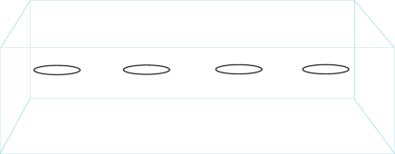
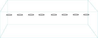
For each , let be a configuration of unlinked oriented circles in a box in . We will fix so the -th loop is a circle of small radius in the -plane centred at . (Up to isomorphism it will not matter precisely which configuration we take for .) The loop braid group is a ‘motion group’ for . See for example Dahm [9], Goldsmith [16], Lin [23], Fenn–Rimany-Rourke [15], Baez-Crans-Wise [4], Brendle-Hatcher [7], Damiani [10] and references therein. Or see Appendix 0.C.
In the spirit of the braid category the groups form a natural diagonal subcategory of a motion groupoid (informally speaking, as in [29], except we should stress compact support — in [29] it is proved that a loop braid group is a motion group in a box with fixed boundary). The monoidal structure is indicated by placing one row of circles following another, to make a longer row: .
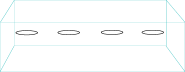
The braid category is the diagonal groupoid whose groups of morphisms are the ordinary braid groups. In this context the braid groups have various relevant realisations (for representation theory it is convenient to work with efficient presentations, but for intuition and application geometric realisations are more useful). In [26] a realisation as hair-braiding is used. In this case one may consider a square (or other topological disk) that is a fixed-height section through the hair, thus cutting the hair at points in the square. An initial configuration, say, places the points at regular intervals in the square. In our loop-braid case the square section through a 3d braid-laboratory is replaced by a box (it would be a section through a 4d loop-braid laboratory), and the points by circles, as in Fig.2.

In the braid case one can either think of the braiding as taking place over time (particles move in the square and world-lines braid), or acting by physical continuity on the hair above the point of action - between this point and the fixed scalp as it were.
In the former perception, we can visualise the braiding by showing all the locations visited by each point - still just drawn in the square. An ‘overlay’ visualisation. This has the drawback that the same location can be visited at different times (indeed a simple static point is an extreme form of this), but the merit is that the visualisation remains in 2d. The drawback can be minimised by only drawing ‘simple’ changes 333Here we will leave the simple-change notion entirely informal and example-based. Note that the separation between two ‘particles’ in some intermediate moment can be small, so simpleness is not necessarily enough to render distinct paths from to homotopic in the relevant space. in a single instance [30]. For this it is convenient momentarily to break out of the diagonal groupoid with object set and into the more general, in the sense of considering partial braidings, passing to configurations different from . Collectively the braidings and partial braidings are ‘motions’. (Depending on the realisation, a motion may be an object set trajectory, or a path in a space of homeomorphisms of the ambient space that restricts to this trajectory. Here we focus on describing the object set trajectory.) The morphisms in the category (the elements in the groups) are certain equivalence classes of motions - see below.
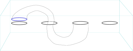
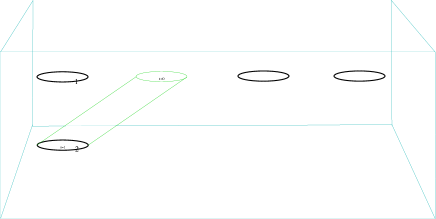
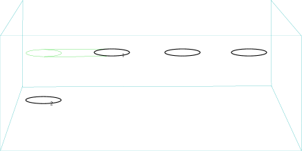
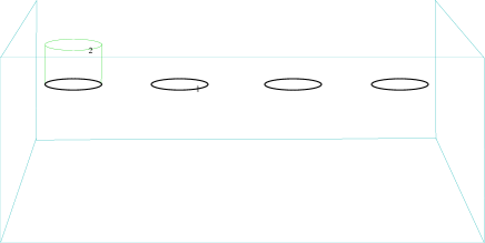
In the loop braid case we thus have overlay visualisations in 3d. We can further use artists-impression to indicate these 3d objects on the 2d page, finally giving representations like those in Fig.3 and Fig.4. Here the colour-code is green for the initial and intermediate points, and black for the final points. Note in this visualisation that the ‘world-line’ of a static point is simply a point.
Two ‘motions’ between the same initial and final configurations (configurations and , say) are equivalent if one can be homotopically deformed into the other in the box. This is a process that is not made easy to track by the overlay picture! (Cf. Fig.4.) But this will not be an issue for us here. Note that the specific figure illustrates one analogue here of the triangle equivalence of polygonal knots. By another such analogue, the image of a circle at some intermediate point in a motion need not be a simple translate of the circle. Examples of this follow shortly. (However see (6).)
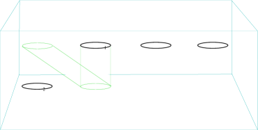
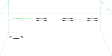
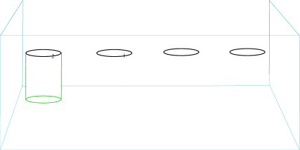
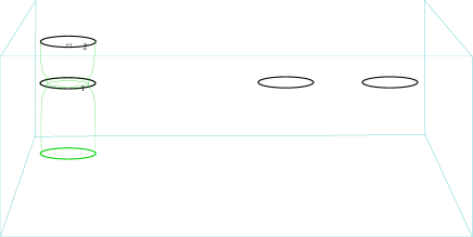
Consider also the the sequence in Fig.5. This sequence is a complete one, in the sense that we finally return, set-wise, to the starting configuration. Similarly Fig.6. Note in general that two motions are composable if the tail of one is the source of the next. A visualisation of the composition would amount to overlaying and replacing all now-intermediate black to green (but we will not need this).

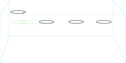
(2.1) It is a useful fact that for each loop every equivalence class of motions contains a representative in which loop is at most translated during the motion (i.e. circularity, attitude and size are preserved). N.B. this is certainly not true for any pair of loops.
 =
=
(2.2)
Here the loop braid category is the
‘category of loop braid motions’
(strictly speaking a subcategory of the category
of all loop motions), as follows.
Let denote the class of
motions in which two loops are exchanged
by one ‘passing through’ another,
as in Fig.6 (ignoring the extra two loops).
Let denote the class where the two loops
pass around each other, as in Fig.5.
Then is the category generated by these motions
and inverses.
(This does not include motions in which a single
loop undergoes an orientation-reversing flip.)
The monoidal composition is as indicated in
Fig.7.
We will not need to dwell on this beautiful but technical construction in order to do representation theory, because we have the following isomorphism (3). Indeed the main reason for recalling aspects of the construction of here is to grasp why the presentation given by (3) takes the form that it does.
3 The setup, and the story so far
We study natural monoidal functors , that is monoidal functors such that . A strict natural monoidal functor is called -charge-conserving. Next we explain how to work with ; explain key properties of ; and hence explain how to give a functor .
A presentation for the loop braid category as a strict monoidal category may be given as follows.
(3.1) The category is the strict monoidal (diagonal, groupoid) category with object monoid the natural numbers, and two generating morphisms (and inverses) both in , call them and , obeying
| (2) |
where (as a morphism) 1 denotes the unit morphism in rank one;
| (3) |
where and ,
| (4) |
Note that because of (2), relation (4)(III) is equivalent to . On the other hand the ‘reverse’ of (4)(II) is not imposed.
(3.2) The map on generators of to given by and (recall (7)) extends to an isomorphism. (For the motion it makes a difference which loop is which, leading to the asymmetry of (4)(II), so later we will be careful with conventions.)
(3.3) By (3) we may simply consider the representation theory of . Or equivalently, we have a representation of provided that the images of and obey identities corresponding to the presentation of above. In practice we will simply identify the two categories henceforward.
Just as a strict monoidal functor (or to any target) can be given by giving the image of the elementary braid , so a functor can be given by giving the pair
| (5) |
(here is some label for the representation). We discuss this in more detail in 0.C.2. The pairs that follow in §5.1 et seq thus give functors in this way.
(3.4) An initial organisational scheme for solutions is provided by the classification on restriction to , as in [26], so we recall this briefly in §3.2.
The foundational aspect of this is the category itself, which we recall briefly in §3.1.
3.1 The story so far: categories
Here is the monoidal category of matrices over a given commutative ring . We take . (See (4.2) below for monoidal product conventions.) For let .
A natural monoidal category is a strict monoidal category with object monoid freely generated by a single object. Recall from [26] that denotes the natural monoidal subcategory of generated (in the obvious sense) by the object in (renamed object 1 in , with ).
(3.5) The index set for rows of a matrix in is the set of words in , and similarly for columns. We sometimes write to emphasise that the word is being used as a column/row index.
A matrix is charge conserving if implies that is a perm of . That is for some , where symmetric group acts by place permutation.
(3.6) The subset of of charge conserving (cc) matrices forms a monoidal subcategory (see for example [26, Lem.3.7I]) denoted .
(3.7) Lemma. [26, Lem.3.7III]
For each and each injective function
there is a monoidal
functor given
on morphisms by
( say).
In particular we have a group action of the symmetric group on .
∎
Example. Consider the nontrivial bijection . On this gives
| (6) |
(3.8) Let be a natural category, as in [26]. For its image under a functor with will be some . Let denote the (simplicially directed) complete graph, as in [26]. The (possibly) nonzero entries in are in correspondence with assignments of a scalar to each vertex of and a matrix
to each directed edge. Altogether for we have
| (7) |
(3.9) Recall from (5) that to give a functor it is enough to give the images and . Here we assume the object map , so and .
For giving is easy to do explicitly, as in (6) or (7), but for general it can be helpful to view elements of geometrically, using the complete graph , as in [26]. The point is that the non-zero elements of break up into and blocks, with the former indexed by vertices and the latter (the submatrix associated to and ) by edges of .
Alternatively we may encode a fixed as a list of the scalars followed by a list of the matrices in a suitable order. For our pair of matrices , thus giving a functor, we will use:
| (8) |
That is, to each edge of we will associate two matrices, giving and , and so on, giving this way.
3.2 The story so far: classification of braid representations
The classification of braid representations we need can be given in rank indexing either by the set of two-coloured multitableaux; or, working up to the symmetry, by the set of multisets of two-coloured compositions, of total degree [26].
In rank for example these multisets may be written
For each index there is an orbit of varieties of solutions. A variety is obtained (complete with named variables) by numbering the boxes of up to order within rows. (We will recall them explicitly shortly.) The size of this variety depends on whether one wants to give representations up to ‘gauge’ isomorphism (i.e. a set of representations that are a transversal of isomorphism classes) or all representations. The former is natural for itself, but since extension to will restrict the symmetry of isomorphism it is natural here to consider the latter.
We will retain the convenient language of [26]. Thus an individual composition in a multiset is a nation; and a part in a composition is a county.
The rank and cases will be particularly important for us. In rank the six varieties have convenient special names. Case — a single county in a single nation — gives rise to the trivial or 0-variety of solutions. Case is the /-variety. Case is the -variety and (depending on box numbering) -variety. Case yields the -variety and -variety.
(3.10) We now recall explicitly the classification for of all which satisfy the relation (4 II), i.e. the complete set from [26, Prop.3.21] of cc braid representations in rank . We have six families of solutions given here. In each of the following families all variables must be non-zero. Organisationally we also insist that in the last four cases since the subset is included in the family of solutions; and similarly in and cases as this is included in the cases and respectively.
| (9) |
The parameter , where it appears, is here ‘unphysical’, i.e. it can be changed by X-symmetry (discussed in §4.1) and does not affect the spectrum. In contrast for say, all affect the spectrum. To match the ‘gauge choice’ made in [26] we should set in (and here is there); and in other cases.
The aim of Section 5.1 then is to establish which of the above braid solutions extend to loop braid solutions. Precisely, given an of one of the above types, when does there exist an such that all (2), (3), and (4) are satisfied?
(3.11) In case we have (from [26, Prop.5.1]) the braid multisets
corresponding to the braid solutions as recalled in (0.A). There are also , , and , treated in [26] by using the additional flip symmetry.
The main point in extending the
braid solutions to loop braid
is going to be to
note from Lemma 5.2
that extension at each edge
is, up to sign, either by an identity matrix
(extending type 0) — so that the vertex eigenvalues
at each end are forced the same;
or by a signed
permutation/
matrix where
the vertex signs are either forced different
(type ) or nominally free (type /);
with no extension for type .
We will thus see the following rules:
1. In the same county vertices must have the same sign;
2. In different counties in the same nation the signs
are different (hence there are at most two counties
in a nation);
And a ‘non-rule’: Vertex signs are not constrained between different nations.
4 Preparations for calculus in Match categories
Both to prove the main Theorem, and the key Lemma, we will need to be able to compute in Match categories. Here we develop the required machinery.
(4.1) Let be a monoidal presentation for a strict monoidal, indeed natural, category . We say a relation has width if it is in . For example the relation (4(II)) above has width 3. We say the presentation has width if is the maximum width among relations in . For example the presentation in (2-4) has width 3.
(4.2) Let be presented by . We may give a monoidal functor by giving the images of the generators. A function from generators to gives a functor provided that the images of the relations hold. The image of each relation say can be checked by checking where the ‘anomaly’ (we assume linear).
As noted in (3.1), a basis element of the space acted on by is , . By the cc property every for some scalars , indeed for every , , i.e. the action on breaks into orbits. Thus:
(4.3) Lemma. The image of a relation of width is verified if and only if it is verified on each subspace , the subspace of the subset . We note that this is the same as verification on up to relabelling, for each subset. I.e. the same as to say that restricts to a functor on each subset. (But note also that the various subsets interlock, and every restriction must hold.) ∎
(4.4) Remark. Note that the monoidal presentation (2-4) has width 3. Thus a pair as in (5) induces a functor if anomalies vanish in every restriction to .
Specifically for say — with (as in 8), say — every term in the anomaly acting on is a cubic with indices in . E.g. , when .
4.1 X-symmetry
Let be a natural category (a strict monoidal category with object monoid freely generated by a single object, denoted 1). The proof of the X-Lemma in [26] observes that if is the image of a generic element in under a functor — thus with elements and so on — then the braid anomaly
has entries that are cubics in the various indeterminate
entries in ;
but in particular in each entry we have one of the following (writing for and so on):
(or ) appears as an overall factor;
and only appear in the form .
Each of the three factors in a term in the cubic come, note, from one of the three factors in a term in . Now suppose we have a second element in , with entries and so on. Then in , say, one of the factors in each term in a cubic will now comes from , so the cubics are modified by some becoming and so on. We observe that simultaneous conjugation by an invertible diagonal matrix still preserves equalities for such cubics. The general X-Lemma follows immediately from this.
(4.5) Lemma. Let be any invertible diagonal matrix (hence ) and be any pair. If induces a functor then so does where and . ∎
A more explicit proof is given in §0.B.
This construction gives an action on the set of all functors, denoted (see also (7.3)), of the abelian group of invertible diagonal matrices.
This action together with the action of (the bijections from (3.1)) generate a group of symmetries of , that we can call ‘core symmetries’.
4.2 Ket calculus: conventions
(4.6) Recall (see e.g. [26]) the convention that the (and hence ) categories use the Kronecker product in the Ab convention. The Ab convention is as indicated by:
(In fact either convention is fine, but we need to fix one. Note that Maxima and MAPLE use the aB convention by default.) This means in particular that the ordered basis 1,2 of (specifically we might take , , although even this is a choice) passes, for , to order 11,21,12,22 with earlier indices changing more quickly. That is . Thus without further adulteration
| (10) |
For we have and so on. 444 In [26] the notation is used, and different conventions are adopted. The choice of conventions is, in any case, essentially unimportant there. But here we must be careful.
4.3 Back to generalities
(4.7) Let denote the identity matrix in . Given then define
| (11) |
In particular this yields the braid anomaly matrix by substituting .
In general for we will write and . So then .
4.4 Calculus via sums of monomial matrices
(4.8) Supposing that is fixed, let denote the simple permutation matrix in , given by for all ; and the identity matrix in . Indeed for given we may simply write for and for .
Note that one way to resolve into a sum of two monomial matrices is
| (12) |
where the diagonal matrix has zeros in the positions and the diagonal matrix does not. Thus for example with :
| (13) |
so
| (14) |
(4.9) Consider the case . A useful observation is
| (15) |
where is given by swapping the 12,12 and 21,21 entries and so on, so here and .
So for example in the simple monomial case, with and , say, then
| (16) |
can be ‘straightened’ by promoting the second . Of course the tensor product affects the promotion.
For example with , and naming variables by: , , , the product in (16) becomes
| (17) |
Thus
(note again the chosen variable names) can be ‘straightened’ by
Meanwhile
From this elementary warm-up exercise we observe immediately that the permutation factors in and agree: , so that for example, we have the following.
Lemma 4.10.
Fix and . For all and (including singular)
| (18) |
Proof.
First consider the case . Compare the diagonal factors in the evaluations of and above and note that in the present case so , , so and so on. Thus (18) holds in this case.
Now suppose we turn on the diagonal terms in (14) for . Thus , say. Of course from the established case of (18) so the full version requires to vanish. Again by the established part of the Lemma we have , so (using established special case at the last step) as required. ∎
Thus in particular we have, for each , a solution to the braid relation by putting , but we also have solutions to the mixed relations for any of the more general form.
5 Rank loop braid solutions
We will prove here that there are three kinds of solutions in rank , given in Lem.5.2.
(5.1)
A couple of organisational principles are convenient to have in mind for spin-chain braid representations
.
These are derived more or less directly from [26]
(and familiarity with this
paper will significantly help the reader here).
(P.I) Each braid representation in rank
restricts to a representation in lower rank by taking a subset of indices .
Thus in particular each representation
with restricts to a collection of representations
(just as complete graph restricts to a collection of s).
And these representations
fall into one of six types:
0, /, , , ,
(recalled explicitly in (9)).
(P.II) Noting that each braid representation
is given by parameterised by
we note (a)
that either is a scalar multiple of
the identity, or at least one of vanishes;
(b) that are eigenvalues, and
is the sum of the ‘middle two’ eigenvalues.
(P.III)
Restricted to the generator our must give a braid representation that is also a representation of the permutation category — of symmetric groups.
In particular so the Jordan form of is
diagonal.
For with its
middle has eigenvalues
or ,
or eigenvalues .
Thus either it is up-to-sign the identity matrix
— whereupon we have , type 0 by the
classification;
or else its diagonal entries obey
and hence (cf. (P.II))
— type /.
(P.IV) By the X-Lemma (see (4.1))
each X-orbit of solutions has a representative where the
nonzero off-diagonal elements of are all 1.
5.1 Rank loop braid solutions: main Lemma
Here we give a complete set of solutions in rank :
Lemma 5.2.
If
gives a loop braid functor
then it is one of the following
(organised according to the braid representation type
of ).
(I) If
is of type
or type
then must take the form
where
for some ,
up to overall sign.
Then for each specific such , i.e. each ,
we get a type solution if and only if
for some we have
.
And similarly in type .
Note this means that
the braid “gauge” parameter in
(9) is locked to .
In particular if we want again to be free to choose
then is forced; and if we want to chose (to set say, see later), for given ,
then
is not free.
Note by invertability and in type or .
Note, in this case
.
Applying from (6) we get
and
.
We can bring this back into the previous form by applying the homomorphism given by
and taking a new given by .
Since (almost) all give solutions,
interchanging them takes us to a point on the same variety,
then giving
,
which, with the restored ,
is thus a viable parameterisation for type .
(II) If is of type or
there is no solution.
(III) If is of type 0
then ,
and there is no further constraint on .
(IV) If is of type / then
where
for some ,
up to overall sign,
and then
with the four further variables
non-zero but otherwise free.
Note
these variables
are independent of .
To match (9) we put
and ,
so
so and
.
The parameterisation has been chosen so that
again captures the X-symmetry, while
are
‘physical/non-gauge’ in the sense that
(unlike ) they do affect operator spectrum.
In particular
.
Proof.
Observe that all possibilities for are considered, by (9), so it remains to verify the extensions in each case and determine any further constraints on . First consider the general form of . The braid classification as in (9) applies to , and (5)(P.III), so is type 0 or /. In cases (I), (II), (IV) , so from the identity (4)(III) we have that cannot be the unit matrix (or minus) here. So by (5)(P.III) we have that where for some and some sign, up to an overall sign. Conversely in case (III) must be type 0.
Cases (I) and (II):
Here we consider of form
where
and
for given and suitable . This is the most general form, but we know in particular from (5)(II) that . For this case of , then, the RRS anomaly here takes the form
| (19) |
Expanding (19) we get
where the first cancellation follows from 4.10; and the because by [26] in type or we have (or indeed for or which cases we can treat by symmetry).
Keeping to the case for now, the first term we need to compute is thus
while the second is
then
and
Observe from the factors that must cancel ; and must cancel . Necessary and sufficient in both cases are:
| (20) |
Here and so and , so . Since is determined by we are in type not , so so the relative sign in is forced as given in the Lemma; and and is as given. This concludes the proof of (I) and (II).
Note that if we want to fix in case (I) (using the X-symmetry as in Lemma 4.1) then (having also fixed that and determined then that ) we also fix and . The only way to vary these latter two is to vary in .
Case (III):
Notice first that in each case, (2), (3), and (4) are clearly satisfied. With of the form , writing the ansatz
| (21) |
then (4 II) gives , hence
We immediately read off and . With , this gives the result.
Case (IV):
From the first paragraph, any exist extending the variety, they are also in the variety.
6 Constructions for the main Theorem
Our task here is first to give certain combinatorial sets and for each rank ; second to give a parameter space for each ; and third to explain how each element and point in parameter space yields a decoration of the complete graph , that encodes a pair of matrices in , and hence formally a monoidal functor Finally we must prove that this pair indeed gives a functor, and that all such functors arise this way.
Again following [26], we can enumerate solutions in two ways. One is to give all solution varieties; and the other is to give a transversal up to the symmetries manifested by Lem.3.1. (Recall, e.g. from [26], that the absolute notion of isomorphism is less straightforward for monoidal-category representation theory than for Artinian representation theory. Our objective here is not to give a transversal with respect to some ultimate notion of isomorphism, but to understand all representations, taking advantage of the isomorphisms that serve this practical end.)
6.1 Index sets for enumerating solution varieties
Here we construct the index sets , and corresponding parameter spaces (we match to actual solutions in §6.2).
(6.1) Recall from [26] that for braid representations in rank- we start with a partition of the vertices of , calling the parts ‘nations’. We then partition each nation further into ‘counties’. In [26] the counties are ordered in each nation and partitioned into two subsets. The set of such structures is the set (whose elements are visualised in [26] as collections of two-coloured composition tableaux).
In our loop-braid case we find that, in order for a braid representation to extend to loop-braid, we must restrict to at most two counties per nation. The counties in each nation are ordered, so this amounts to the choice of a (first county) subset for each nation. (We then colour the counties from two colours, but in our case the colours are forced.)
Next comes the new ingredient that is not merely a restriction, which is that a subset of the nations is chosen (those that will be associated to +, i.e. +1 eigenvalue of for individuals in the first county).
The above features characterise the loop-braid index set . It is useful also to give a more formal construction for as follows.
We continue to use notation from [26]. And we add a few more devices. In particular for a set, denotes the set of partitions of into an ordered pair of parts (thus is in bijection with the power set ). Example:
And the subset of these in which the first part is not empty. Further, given an indexed set of sets that are disjoint we write for the set whose elements are sets made by selecting one element from each .
Given a partition of let us write
(thus the set given by the choices of a non-empty subset of each part , whose elements are the collections of pairs where ). Examples:
(hopefully a multi tableau visualisation is easier on the eye - here specifically the multi-tableaux consist only of single tableau); and for a case requiring a proper multi-tableau:
Altogether then we have a set
where is the set of partitions of . It is convenient to draw nations and their counties - ordered two-part set partitions - as composition tableaux (cf. e.g. [36]). And collections of nations as collections of tableaux. So for example
(note the last set contains only a single composite element, drawn as a sequence of two nations, although this drawn order has no significance). For an example of an element in larger rank we have
| (22) |
This raises the question of how to order the nations in drawing such a picture. This is unimportant here but useful later. Later we order with smaller nations first; and then larger first counties first.
(6.2) Finally
Example:
(6.3) The symmetric group acts on by application to the individuals in the counties.
The shape of an element is the diagram obtained by ignoring the entries in the boxes. Note however that these combinatorial objects are multisets rather than sets. (As we will see, they are both beautiful and useful. We study them in §6.3.)
It will be evident that a transversal of the orbits of the action is described by the set of shapes. (In §6.4 we give a way to convert the set of shapes into a ‘standard’ transversal in .)
(6.4) We fix the ground field . Associated to each there is a ‘type-space’, call it . There is a non-zero parameter for each county - we require for the two parameters in the same nation; and a pair of non-zero parameters for each pair of nations.
Let denote the set whose elements are pairs where and is a point in .
6.2 Recipe constructing (all) representations
Here we give a construction for varieties of cc loop braid representations (Theorem 7.3 will show this is gives them all). The varieties are indexed by , and describes the parameter space of each variety.
(6.5) It will be helpful to give names for the individual parameters in . To this end we can order the nations (i.e. composition tableaux) in , , as follows — order first into the ordered pair; then within each component using the natural order on nation sizes; and then at fixed size using the natural order on second-county sizes. Finally the repeats of a given shape are ordered child-first (i.e. nation with lowest numbered resident first).
Now for each nation fix the two non-zero parameter names , associated to the first (upper) and second county respectively. (Recall we require in addition that .) For each pair of nations with fix the two non-zero parameter names and .
(6.6) Next we give a construction for each of a function
| (23) | ||||
| (24) |
We will show that this gives all charge conserving loop braid representations.
(6.7) For we encode in by as in (8); and by . To give a solution we give the scalars , and matrices , for all . These depend on the relationship between the counties/nations that individuals reside in. Specifically:
Consider each individual . Let be the nation that resides in. If is in the top county in then . If is in the other county of then . If comes from the first (resp. second) part of the pair then the ‘sign’ of is (resp. ). If the sign is and is in the top county then ; while if the sign of is and is in the second county then . If the sign of is then the cases are reversed.
Consider each pair of individuals .
(We proceed
as in Lem.5.2 but choosing the
gauge/X-symmetry
parameters , adopting the principle that off-diagonal elements of are gauged to 1.)
-
1.
If and with then , and — here if arises with it is to be understood as .
-
2.
If and are in the same nation but different counties with in the top county then 555Alternative version: and . — note this works but diverges from our gauge choice. and . If is in the top county then and .
-
3.
If and are both in the top, respectively bottom, county in then , respectively ; and .
(6.8) Example. For we have
(RRR, SSS, RSS, RRS all hold and, as desired, SRR does not - these are somewhat large but routine calculations; we omit the details, but see [27]).
(6.9) Example. For we have
Observe that this is also (6.2) with with applied, cf. (6). So again RRR, SSS, RSS, RRS all hold and, as desired, SRR does not, without further checking.
(6.10) Non-Example. For we do not have a solution taking
(which are riffs on a first draft recipe, but both sign versions are checked as RRR:True; SSS:True; RSS:False! in [27]).
(6.11) Example. For we have:
(6.12) Cautionary Example. For we do not have
(RRR, SSS, RSS, all True; but RRS false with these signs - see [27]. Of course it will work with all off-diagonals in , since this is just from (6.2), but this does not adhere to our gauge choice).
(6.13) Example. For we have
(RRR, SSS, RSS, RRS all True).
(6.14) For we have:
so , so this works. Meanwhile for we have:
so .
(6.15) Note from the construction of that counties are unordered sets, thus permuting the indices within counties does not change the element of . It is straightforward to see from the recipe that the map is well defined with respect to such a permutation.
6.3 Index sets for -orbits of solution varieties
Here we give the construction of the set (the set of shapes from (6.1)). There is an injection of into , thus there are again varieties of pairs associated to each member of . We will show in Theorem 7.3 that, up to symmetry, this subset is sufficient to give all charge conserving loop braid representations.
We start by codifying the set of shapes.
(6.16) Recall that a multiset on a set is a function (assigning a multiplicity to each element); and that if is a degree function on , then is the set of multisets that have total degree .
A signed multiset of degree is equivalent to an ordered pair of multisets of total degree (the first multiset gives the multiplicities of objects signed +; and the second signed -). Let us write for the set of pairs of multisets as indicated. So the set of pairs whose total degree is is .
(6.17) As we will see, our indexing combinatorial objects at rank are signed multisets of compositions into at-most two parts of total degree .
Write for the set of at-most two-part compositions — equivalently the set
| (25) |
Note that the number of elements of of degree is ; and note the total order indicated by (25). Here write just for . The ordinary multisets are ;
and so on, writing to indicate for a given function that , with other multiplicities 0.
(6.18) For the signed versions, where: and . Then where
Next with
Next with
and so on.
6.4 Recipe constructing all representations (up to symmetry)
Here we give an injection of into . We thus give, via , a construction for varieties of cc loop braid representations up to symmetry (Theorem 7.3 will show this is gives them all).
(6.19) Recall that a multiset can be considered as a set but where entries can be repeated, or indeed missing (in this perception the repeats must somehow be given individuality from each other, for example if then we have copies of individuated by , perhaps). Given an order on the underlying set we can write the set form of as a sequence. Individual terms that are repeated elements then receive ‘individuality’ from their identical siblings by their order in the sequence.
(6.20) Following on from (6.4), an ordered pair of multisets can then be seen as an ordered pair of sequences (or, say, as a sequence where each same-type run is partitioned into two, but we will adopt the former organisation).
In this way gives an ordered set of nations (i.e. compositions) — ordering first into the ordered pair ; then using the natural ascending order on nation sizes; and then at fixed size using the total order on from (25) i.e., in ascending order by the size of the second county). Finally the repeats of a given nation are of course nominally indistinguishable, so simply ordered as written.
(6.21) Example: Suppose is given by and and others zero; and by and and others zero. Then can be represented as
| (26) |
Thus here, in this pair-of-sequences form, , , , , , .
(6.22) Given ordered as above we obtain a composition tableaux in by filling in the numbers in order, with the first numbers going into from left to right and then from top to bottom. From the example above we see that (26) then becomes:
| (27) |
This gives an injection of into , so we may identify with the unique order preserving composition tableaux obtained as above, and abuse notation. Let denote the subset of coming from the image of , i.e., pairs with .
Now we may apply the recipe (6.2) to to obtain a solution. We will see that, up to -symmetry and symmetry, every rank solution is obtained from an element of .
(6.23) See 0.D for examples.
7 Main Theorem
7.1 Prelude to the main Theorem: a key Lemma
(7.1) Lemma. Let be any pair as in (5). Then induces a functor if and only if every restriction to rank 2 is a functor (i.e. belongs to the list in 5.2); and the restriction to is a functor (i.e. every restriction to rank-3 belongs to the list in 0.A up to symmetry - where we here use Lemma 4 to pass to rank-3).
Proof.
By Lemma 4 (and Remark 4) it is enough to verify in case . Thus it is enough to consider all extensions of the set of functors . These are reproduced in (0.A). A nominal superset of these is given by extending in all nominally possible ways, according to 5.2, at each edge. The complete enumeration of possibilities proceeds as in (0.A). This finite set of groupings of cases is then verified by routine if lengthy direct calculation (or see e.g. (7.1)). ∎
(7.2) Proof. (Alternate) We may verify explicitly by checking that all cubics in rank obtained from (33) with , and with (i.e. for (3)(II) and (III)) are satisfied for each matrix satisfying the assumptions of the Lemma. It is assumed that each is a representation of for every restriction to rank , thus cubics containing a repeated index, e.g. , are assumed to be satisfied, and we only need to check equations in the permutation orbit of (34)-(38).
Recall that, as explained in 3.1, rank solutions are represented by the complete graph with rank solutions attached to each edge. We organise our sequence of checks by the number of restrictions of to rank solutions that are edges. The corresponding edges in are then of type or , with various conditions as in (0.A). We start with the case that no edges are , then the case all edges are . We then divide the remaining cases into the relations (3)(III) and (3)(III), which are each subdivided by the number of edges. In each case we show that the permutation orbits of each of (34)-(38) are always satisfied.
Suppose first that all restrictions of and to rank solutions are in the zero varieties. Then all off diagonal entries are zero, it is thus immediate that all terms in the orbits of (35)-(38) go to zero. For (34), notice that , since, by considering the Lemma 5.2, each matrix is a multiple of the identity matrix.
Now suppose all rank restrictions are of type, then all diagonal entries are and all equations trivialise.
We now consider the relation (3)(III), so let in (34)-(38), in particular we use capital letters to refer to elements of and lower case to elements of . It is immediate that (37) is trivial after this substitution. We then further replace lower case elements with greek letters to avoid confusion between this and denoting the gauge parameter in Lemma 5.2.
Now suppose that restricts to two solutions in the variety, and one in the zero variety. By symmetry, we may assume that the solution in the zero variety lies on the edge. First notice that for all distinct , since the or the edge is in the variety. Thus, looking at (34) we must have that, for all distinct
If is a edge, . Otherwise is the edge, i.e. , and in both cases the condition becomes . Let us now explain our notational convention: we use the parameter labels from Lemma 5.2 for each rank matrix, and, where necessary, add a subscript to indicate the edge. Looking at (0.A), we have two cases. The first is that the and edges in are -type, in which case all parameters from Lemma 5.2 are locked equal across the edges by (0.A), and the condition becomes . The second case is that the and edges in are -type, in which case the and parameters from Lemma 5.2 are locked equal across the edges by (0.A), and the condition becomes .
Using again that , (35) becomes the condition . If is zero edge we are done, so suppose not. This gives . Both sides go to zero if is a , so suppose not. This means , and in both cases we have , which is again true by observing that solutions are locked equal.
We now consider the relation (3)(II). We show that all cubics (35)-(38) are satisfied for the case , i.e. capital letters now refer to elements of , and greek to elements of . Note we have already done the case that all restrictions of to rank solutions are in the zero variety. Also (38) becomes trivial.
Suppose restricts to two solutions in the variety, and one in the zero variety. As above, we may assume that this zero solution is on the edge. We first prove that (34) is always satisfied.
Suppose first that is the zero edge, thus . Then (34) becomes . Since is the zero edge, , thus it is sufficient to observe that becomes as and this is satisfied by the locking together of pairs of and type solutions.
Now suppose is the zero edge, thus , and (34) becomes . If restrictions of to the and solutions are in the variety, both sides become . For the restrictions there are two cases, the first is , for which we have either , or . These correspond to the two cases for the fourth triangle in (0.A). The other case is similar.
Finally for the case is the zero edge, then , and, since , and all terms in (34) go to zero. The arguments for (35),(36) and (37) are similar.
Finally we consider the case that all edges of are of type, and has two edges of type and one of type. We will assume the type is the edge . Notice first that (38) becomes trivial.
First consider (34). This becomes Now either is zero, or is the edge, and we have . Equations (35) and (35) all go to zero by noting all terms contain either of diagonal elements of , or pairs of diagonal elements from distinct edges of . Equation (37) becomes , and we have either , or is the edge and the condition becomes which follows from the locking together of pairs of edges in (0.A). ∎
7.2 The main Theorem: statement and proof
Theorem 7.3.
(A)
(I) The construction gives a
charge conserving
monoidal functor
for every .
(II) Every such
functor is in the orbit of some
under the X-symmetry (of 4.1).
(B)
(I) The construction gives a
monoidal functor
for every .
(II) Every such
functor is in the orbit of some
under the and X-symmetries
(of 3.1 and 4.1 respectively).
7.3 (AII) Proof
(7.4) As in [26] we write for the category of (monoidal) functors. Let us write simply for the object set. Consider an arbitrary such functor , and hence the pair , . We will determine the such that up to gauge choice. We do this below by interrogating for a suitable ; and then further for a suitable . (This parallels the case, where we interrogate for a suitable and so on.
(7.5) Recall from (6.1) (or [26, (4.4)]) that is the set of all two-coloured multi-tableau on boxes. Recall that is the recipe constructing varieties of braid representations from .
Let be any braid representation. Observe from [26, (4.7) and §6.3] that the element of associated to is given by (all component functions as defined in [26]). Let us now write for this element. That is, is the variety containing up to gauge (in this way it was shown that constructs all representations).
We will modify the pseudo-inverse function for our case.
(7.6) In our case firstly note that since, by Lem.5.2(II), there are no edges (still in the sense of restricting to the braid solution part) the ‘colour’ must differ between every pair of counties in each nation of . There are two colours, so this forces that there are at most two counties in each nation, always of different colour. - So, note, we do not need to further record colours. This can be realised as a set of composition tableaux — tableaux where order in a row does not matter (so we can use natural ascending order for free), and order between rows does matter. For examples:
| (28) |
In such representations as these the nations also appear arranged as a sequence rather than just a set, but so far this is arbitrary, cf. (6.4).
(7.7) Recall from (6.1) that denotes the set of partitions of such sets into an ordered pair of subsets, restricting to the case of compositions with at most two parts (two parts of different colours, in the original idiom).
(7.8) We define as the partition of into an ordered pair of subsets, with nation in the first part if for the individual in the top left box of nation .
(7.9) For example perhaps:
| (29) |
For an example of large enough rank to be generic (but still neat to typeset!) we use instead of :
(7.10) Having interrogated for a , we now interrogate for an .
Associated to each nation , say, of there are and values that can be read off from — inspecting gives either or for ’s nation, depending on whether is in the first or second row. Observe that in the same row have a type-0 edge between them here, so the procedure is well-defined without specifying further.
Associated to each pair of nations, with , there is a parameter value, given by square root of product of off-diagonals in between any in and in . Observe again well-definedness.
Continuing with this , we can also read off the value of . This does depend on , but the value of is determined from the off-diagonals in , i.e. , so we can determine . Note that we can apply X-symmetry to to make in all cases. To be precise, in case ,
| (30) |
(recall that , for example, is the bottom left entry in the matrix corresponding to the edge). If instead then
| (31) |
Observe that the operator spectrum depends on but is invariant under .
Write for this collection of parameters. Note that there is potential ambiguity in the organisation of the collection, resolved here by the total order on nations, as in (6.1).
(7.11) We claim that is gauge-equivalent to . (N.B. This implies (AII).)
To see this first note that the restriction to is
correct up to gauge by (7.3).
A couple of examples will suffice to check that no
new gauge issues arise.
1. Suppose .
Necessarily then gives values for two nations, thus .
For all pairs we are in case (30), thus we
know from this and Lem.5.2 that takes the form
for some , with forced. Note that Lem.5.2 puts here, since . And given this then must be
It follows from (6.2) that the image takes the form
Observe that this is indeed
in the X-orbit of , by putting , .
2. Suppose . Necessarily then gives values for two nations, thus . Here we are in case (31) when , and case (30) otherwise, using this together with Lem.5.2 we know that takes the form
for some , with forced. Note that Lem.5.2 puts here, since . And given this then must be
It follows from (6.2) that the image takes the form
Observe that this is indeed
in the X-orbit of , by putting , .
4. Suppose
.
We know from Lem.5.2 that takes the form
for some . And given this then must in particular be
for some values of the parameters. In this case it follows from (6.2) that the image takes the form
This is in the X-orbit taking .
3. Suppose .
The main new observation here is that by the nature of 0-edges.
So again the recipe agrees up to gauge.
∎
7.4 (BII) Proof
Let us write the action of on simply permuting the entries as . For (BII) it is enough to show that the (with notation as in 3.1) and naive actions agree on , since is clearly a transversal of under the dot action.
(7.12)
We claim that
.
(Note that the identity is one of varieties, not of
individual solutions. We can see from the construction
that the size of the variety is not affected by .)
Proof.
Let us work through some specific kinds of cases.
We will be done when we have verified the action of
(generating) elementary transpositions across the
various contexts that arise. Several cases have
already been treated in (6.2) et seq, so
we continue from there.
Note that the corresponding result connecting
and is established in [26].
We must consider under the following scenarios:
1. in the same county;
2. in different counties in the same nation;
3. in different nations with the same sign;
4. in different nations with different sign.
For case-1 both actions are trivial (see also 6.2).
For case-2,
consider applying to our in
(29).
This flips the 3X edge, taking it from type to type
(cf. Example 6.2).
It also swaps the 1X and 13 edges (a 0 edge and an
edge), and leaves all other edges and unchanged.
Looking at the construction of we have that
is
which is immediately seen to be .
For case-4,
suppose we apply to
our in (29),
i.e. as in (3.1).
Then
we claim
is given by
(and cf. (6.2)).
This can be seen by noting the following.
In this new equivalent solution
vertex 1 will have the
the parameter value from the old 9X3 nation, and vertex the parameter from the nation
(so it
is apt
to think of the parameter
staying with the nation under exchange, even though
two nations could entirely swap populations
— we can call
this Mach’s other principle [17]).
Vertex 1 will also have ‘exchanged’ its eigenvalue
with vertex 9
(although this is +1 to +1 so no change, here).
The 0-edge at 9X is now a 0-edge at 1X.
The /-edge at 69 is now a /-edge at 61 (or 16, note that the off diagonal entries will also flip), and so on.
Similarly,
the /-edge at 1X is now a /-edge at 9X.
The edge is now an edge , and similarly with to .
Case-3 is similar.
∎
This concludes the proof of the Theorem.
8 Discussion and future directions
The input to our recipe yields some interesting combinatorial questions.
(8.1) Note from (6.3) that the integer sequence for is the Euler transform of 1,2,3,4,…, which begins 1,3,6,13,… This is also MacMahon’s sequence for plane partitions (since this is the same Euler transform, as noted in [38, OEIS A000219]).
(8.2) Exercise. Determine a bijection!
(8.3) Let us determine the size of by another method. First note that there are exactly distinct compositions of into at most 2 parts. To build the elements of we form a multiset of such compositions so that the sum of their sizes is . The generating function for the number of ordinary partitions is : indeed, partitions can be regarded as a multiset of natural numbers . The modification for our set up is that we are selecting multisets of compositions into two parts, and there are distinct compositions of each size . Thus each factor should be taken times, giving
This indeed coincides with MacMahon’s GF for the sequence of sizes of sets of plane partitions. It is intriguing that the proof here is obtained very neatly from the very classical (due to Euler) ordinary-partitions case. The proof for plane partitions appears far more involved — see e.g. [39].
(8.4) The sequence for is (1), 2, 7, 18, 47, 110, …. This is also the count for the set of ordered pairs of plane partitions of total degree (see e.g. [38, A161870]). Of course if a sequence has generating function (in our case MacMahon’s function) then the sequence for ordered pairs has generating function .
It is an important question as to the measure of the
set of charge-conserving representations in the set of
all representations
up to a suitable notion of isomorphism
(i.e. how restrictive were the constraints we put on in order to get a complete solution?).
One way to think about this is by analogy with the
corresponding problem for Hecke representations.
To this end it is instructive to
compare with the machinery of classical Hecke representation theory
as in [25].
There we see, by a method involving Bruhat orders,
that cc representations are, in a suitable sense, eventually faithful
(note in particular [25, §2.3(7)]).
This raises several further representation-theoretic questions, such as the following.
What is the smallest (monoidal) subcategory of that contains all perm matrices?
What is the smallest that contains all perm matrices
as “additive” components (subblocks)?
Is there a fusion trick?
What about monomial matrices?
This work can be seen as part of a more general programme on Representation theory of natural categories. Here one starts by observing the naturalness/singular-ness of natural categories in the wider realm of monoidal categories (cf., for example, [18]), as way of unifying groups and algebras a la statistical mechanics (cf. for example [28]); and observes key rigidification aspects. Many questions arise here, for example around generalisations and around applications (in particular to topological quantum computation - cf. for example [3, 34, 14, 41]).
Appendices
Appendix 0.A Background for the Proof of Lemma 7.1
The simplicially-directed graph has edge orientations , , . The following decorated simplicially-directed diagrams should be understood as in [26], giving with vertex parameters given by vertex labels, and for example, given by the label on the edge from vertex to vertex .
(0.A.1) Proposition. [26, Prop.5.1] For the following types of configurations yield a charge-conserving functor (showing one variety per orbit):
(0.A.2) For example, the case shown is (second row coloured). In this orbit we have also and , collectively labelled . On the other hand, in the orbit (not explicitly represented above) we have which unpacks to
- note that after the first move the 23 edge decoration is reversed, but the parameters on this edge are now tied to those on edge-12.
(0.A.3) Eliminating from (0.A) the cases with , which by Lem.5.2 do not extend, we have:
with corresponding indices:
Note that we do not know ab initio that any of these extend. The formally possible extensions in each case (according to the application of Lem.5.2 to each subgraph) are represented by giving the corresponding decorations for . We write and for the diagonal eigenvalues . We write for the edge decoration (taking advantage of the gauge freedom to fix this), but to indicate that the vertex eigenvalues are forced opposite. For the 0 edges the vertex eigenvalues are forced the same. Note in particular that the diagonal eigenvalues within a nation are all determined by . Indeed they would be over-determined if there are more than two edges — more than two counties, but this is already impossible. On the other hand the relative eigenvalues between nations are not formally determined. Thus the possibilities overall correspond to a choice of sign for (the lead in) each nation. We have:
together with the overall flips. For completeness (since we have not introduced the flip move here) we should include here, say,
We find by direct calculation that all satisfy the constraints.
Appendix 0.B Ket calculus: the Texas braid relation
Here we give a proof of Lemma 4.1 by direct calculation. In fact, we prove a slightly more general statement:
(0.B.1) Lemma. Suppose satisfy
| (32) |
in (recall and so on). For invertible let and so on. If is diagonal then
.
Proof.
Consider the equation
| (33) |
where with nonzero entries lower case Roman (), upper case Roman () and lower case Greek (), respectively, where . We have (for , with analogous conventions for ):
We will show that if and satisfy equation (33) then so do and .
First note that conjugating each of and by a diagonal matrix leaves the diagonal entries and invariant, while the effect on the other entries is: for and for for some . To see that this leaves the polynomial equations unchanged we compute a few entries. First it should be clear that the entries give trivial conditions. For the entries with distinct it is enough to consider by a local permutation argument: one simply applies the permutation to all indices and then defines, for , , , and and similarly for the and .
We have:
whereas:
This yields 6 equations the last of which is trivial (denoted by (*)):
| (34) | |||
| (35) | |||
| (36) | |||
| (37) | |||
| (38) | |||
Next we compute the polynomial consequences of the generic braid relation on .
Here we have:
whereas
These yield equations, that last of which is trivial:
| (39) | |||
| (40) | |||
Similar computations equating and on and yield:
| (41) | |||
| (42) | |||
| (43) | |||
| (44) | |||
| (45) | |||
Again, we omit the calculations for and as the corresponding polynomial equations can be obtained from the above by applying the transposition and defining , etc.
Now we observe that in each equation either
-
1.
Each term has the same number of or (resp. or ) terms so that the equation obtained by simultaneous -conjugation has a negligible overall non-zero factor, or
-
2.
Each term with a term also has a corresponding term (not necessarily matching) so that the effect of -conjugation is nugatory.
This completes the proof. ∎
Lemma 4.1 now follows by substituting for as appropriate.
(0.B.2) Remark. The superficially braid-like equation (32) seems too general to have such a geometric-topological meaning. Some of its specialisations can be endowed with such meaning, as we can see from our context. But not all. Nonetheless, in it is useful.
Appendix 0.C The loop braid category : technical asides
Here we aim to provide, in support of Sec.2, more of a rough substitute for the braid laboratory of [26] - by working with an appropriate motion groupoid; and hence to give a bit more of a feel for the relations in the presentation (3). And to prove 0.C.14, on non-monoidal presentation.
0.C.1 Topological Background
In what follows we denote the unit interval by . We denote the unit ball and the unit circle .
(0.C.1) Let be a manifold, with boundary , and . Let denote the set of self-homeomorphisms of , made a space with the compact-open topology.
A flow of is a path with and all pointwise fixing ; or equivalently an automorphism such that for each , restricts to a homeomorphism fixing , and such that is the identity.
A motion of taking to is a triple consisting of a flow of , a subset , and the image .
Two motions in , are motion equivalent if can be continuously deformed into through motions taking to .
For each , there is a groupoid with objects the power set of and morphisms from to , motions up to motion equivalence. Following [29] (where all details can be found), we denote this groupoid .
(0.C.2) For some manifold and set of subsets of , we use to denote the full subgroupoid of with objects .
For example, if is a collection of points, for each ; and is the set of all the s, then is a realisation of a braid group, and is a realisation of the braid category. This realisation bridges between the purely presentational one useful in representation theory, and the braid laboratory. Of course the connection to the braid laboratory makes several distinct uses of the continuum hypothesis. What we do next will make several more!
Fix a small number . For each , we fix an embedding of copies of into the interior of such that is a configuration of unlinked circles of radius in the -plane with the -th loop centred at . (Up to isomorphism it will not matter precisely which configuration we take. The present choice is different from the one in the body of the paper, simply because we prefer not to have to unpick here the technical details of the limit required to have both the correct motion group on the nose, and the natural monoidal structure.)
Let be the set of all such . Note that , since morphisms in exist only between homeomorphic subsets of , and, by construction, contains precisely one element in each isomorphism class.
The reader will readily confirm that for each pair there is a function taking to that takes the corresponding to in the spirit of Fig.7 (up to some rescalings), and hence in the spirit of the braid laboratory of [26]. It follows from (0.C.1) that this collection of functions induces a (natural) monoidal structure on , and hence on (rigorous details will appear in [30]). As a brief abuse of notation we will use the same symbols for the monoidal categories.
Let
(0.C.3) Next we consider some morphisms in . We have in mind motions inducing the circle trajectories of type and as in §2. That such trajectories extend to motions as in (0.C.1) could be shown by giving an explicit construction, or proving a suitable isotopy extension theorem, but here we simply lean on the (correct) intuition that there is one. (See [29, §5.1] for brief technicalities. Complete details will appear in [30].)
Let denote a morphism represented by a motion which swaps the positions of the th and th circle, such that the circles remain parallel to the -plane, and such that the th circle ‘passes through’ the disk parallel to the -plane bounded by the th circle. The circle trajectory for such a motion is represented in Fig. 6. (The support of a motion is the set of points that are not static throughout. A key property of motions such as is that they include representatives where the support is localised in the region of and . Thus the local-view Figure conveys the motion - it is recovered by suitably appending and prepending static loops.)
Let denote a morphism represented by a motion which swaps the positions of the th and th circle, such that the circles remain parallel to the -plane, and neither circle ever intersects the disk parallel to the -plane bounded by the other. Such a motion is represented in Fig. 5.
Let denote a morphism represented by a motion which rotates the th circle by about an axis passing through the circle twice and its centre (thus the restriction of the endpoint of the motion to the th circle is an orientation reversing homeomorphism).
The proof of (0.C.1)-(0.C.1) below is essentially contained in [9], and reproduced in [16], although we note that, as pointed out by [42], the proof requires the additional assumption that each motion, and each homotopy, has compact support, rather than just each self homeomorphism. With this additional assumption it can then be shown that the motion group of loops in constructed in [9, 16] coincides with .
(0.C.4) Consider the bouquet of loops homotopic to the complement of in (see e.g. [11] and references therein). Each motion induces an automorphism on the fundamental group of this bouquet. Clearly this fundamental group is generated by the simple loop paths. In fact it is free on these generators (for example by a universal cover argument).
Let be the group of automorphisms of the free group generated by . The given construction yields a homomorphism
(0.C.5) Let us consider the following automorphisms in .
While it is not easy to see that the construction in 0.C.1 yields a well-defined group homomorphism from it is straightforward to see that the images of our motions in (0.C.1) above are these automorphisms, in particular , and . Moreover is an isomorphism onto the subgroup generated by . We thus have the following.
(0.C.6) The elements generate the group .
(0.C.7) Observe that as we have introduced it in the paper obeys . It is the subgroup generated by and , at each .
Intuitively, we are restricting to classes which contain a motion which keeps all loops parallel to the -plane throughout the motion.
It follows from from (0.C.1) and (0.C.1) that there is an isomorphism (see also [9]) from onto the subgroup of generated by the .
The following identities are readily verified in :
| (46) |
0.C.2 Generators and relations
Here we give a little background on two further technical aspects (again not strictly needed for this paper, but useful contextually). One is the nature of functors from finitely presented natural categories; and the other is on monoidal versus non-monoidal presentation.
(0.C.9) Let be monoidal categories, with monoidal identity objects denoted by and , and monoidal composition maps denoted respectively.
A strict monoidal functor
is a functor
such that
,
for all pairs of objects in , and
for all pairs of morphisms in .
(0.C.10) Strong and lax monoidal functors weaken the equalities in Def. 0.C.2 to isomorphisms and morphisms respectively. Specifically a strong (resp. lax) monoidal functor consists of a functor , together with an isomorphism (resp. morphism) and a natural isomorphism (resp. transformation) , with various coherence conditions.
In the diagonal categories considered here, there are no morphisms between distinct objects so the conditions of strong and lax monoidal functors imply the equalities on objects as in Def. 0.C.2. Although this a priori leaves open the possibility of non-trivial automorphisms and .
We can codify the strict monoidal functors from to as follows.
Lemma 0.C.11.
Let be natural monoidal categories such that is finitely presented with non-empty set of generating morphisms and a corresponding set of relations . Of course any functor restricts to a pair consisting of the value of ; and a function . In particular if then . Let , and let be a map sending each in to a morphism in . Then extends to a functor , which is unique, precisely if the images under of the relations are satisfied in .
Proof.
Since generates, every morphism can be built (albeit non-uniquely) as a category-and-monoidal product of elements and identity morphisms. There is an extension of to a formal map , which on objects is the map with , and on morphisms is defined by the relations , , and . This is a well defined map precisely when the relations are satisfied, in which case it is a strict monoidal functor. By construction it is unique. ∎
(0.C.12) Recall that the object monoid of the monoidal groupoid is the natural numbers, and that both generating morphisms are of the form , where =2, and therefore all unless .
(0.C.13) After fixing , we denote the element of length by . We similarly label , and . Notice, using that is a functor and thus preserves composition, that these elements generate the group .
Lemma 0.C.14.
There is an isomorphism of categories (not using the monoidal structure)
which, at each , sends and .
Proof.
First observe that since the , and generate , there is a unique map satisfying the conditions of the Lemma and preserving composition. For this to a be a well defined functor we must check that the relations in (46) are satisfied in . Surjectivity is satisfied since the and generate .
We can prove both well-definedness and injectivity by noting that each relation in (46) corresponds directly to a relation in and vice versa. The relations and when correspond to relations coming from the fact that is a functor. All other relations in (46) correspond directly to the relations (2), (3) and (4). ∎
Appendix 0.D Applying the recipe, and variations, to
(0.D.1) Consider the set of solutions for , thus associated to as in (6.3) by the recipe as in (6.4). Here firstly we have four solution sets associated to (or eight ignoring symmetry):
(we use up the gauge symmetry on and absorb the effect of the gauge choice in free variables );
(here the can be in each position);
and similarly to those above with .
The other two solutions from are given by two and three ’s in .
Note that overall this is every possible way of
extending in each subspace,
given that these solutions interlock at the vertices.
Next we have four solution sets associated to
:
and (with corresponding re-gauging if required).
Four sets associated to :
for example gives
while gives
Two sets associated to :
Two sets associated to :
and .
Two sets associated to :
and .
Note from [26, Prop.5.1] that these exhaust the possibilities for and visit every possibility for consistent with and the interlocking conditions.
References
- [1] N. Andruskiewitsch and H.-J. Schneider. Pointed Hopf algebras. In New directions in Hopf algebras, volume 43 of Math. Sci. Res. Inst. Publ., pages 1–68. Cambridge Univ. Press, Cambridge, 2002.
- [2] E. Artin. The theory of braids. American Scientist, 38(1):112–119, 1950.
- [3] J. C. Baez and U. Schreiber. Higher gauge theory. In Categories in algebra, geometry and mathematical physics. Conference and workshop in honor of Ross Street’s 60th birthday, Sydney and Canberra, Australia, July 11–16/July 18–21, 2005, pages 7–30. Providence, RI: American Mathematical Society (AMS), 2007.
- [4] J. C. Baez, D. K. Wise, and A. S. Crans. Exotic statistics for strings in 4d BF theory. Advances in Theoretical and Mathematical Physics, 11(5):707–749, 2007.
- [5] V. G. Bardakov. Extending representations of braid groups to the automorphism groups of free groups. J. Knot Theory Ramifications, 14(8):1087–1098, 2005.
- [6] R. J. Baxter. Exactly solved models in statistical mechanics. 1982.
- [7] T. E. Brendle and A. Hatcher. Configuration spaces of rings and wickets. Commentarii Mathematici Helvetici, 88(1):131–162, 2013.
- [8] A. Bullivant, J. Faria Martins, and P. Martin. Representations of the loop braid group and Aharonov-Bohm like effects in discrete -dimensional higher gauge theory. Adv. Theor. Math. Phys., 23(7):1685–1769, 2019.
- [9] D. M. Dahm. A generalization of braid theory. PhD thesis, Princeton University, Mathematics, 1962.
- [10] C. Damiani. A journey through loop braid groups. Expositiones Mathematicae, 35(3):252–285, 2017.
- [11] C. Damiani, J. Faria Martins, and P. P. Martin. On a canonical lift of Artin’s representation to loop braid groups. Journal of Pure and Applied Algebra, 225(12):106760, 2021.
- [12] C. Damiani, P. P. Martin, and E. C. Rowell. Generalisations of Hecke algebras from loop braid groups. Pacific J. Math., to appear.
- [13] J. Elgueta. Representation theory of 2-groups on Kapranov and Voevodsky’s 2-vector spaces. Advances in Mathematics, 213(1):53 – 92, 2007.
- [14] J. Faria Martins and R. Picken. Surface holonomy for non-Abelian 2-bundles via double groupoids. Adv. Math., 226(4):3309–3366, 2011.
- [15] R. Fenn, R. Rimányi, and C. Rourke. The braid-permutation group. Topology, 36(1):123–135, 1997.
- [16] D. L. Goldsmith. The theory of motion groups. The Michigan Mathematical Journal, 28(1):3–17, 1981.
- [17] S. Hawking and G. Ellis. The large scale structure of space-time. 1973.
- [18] A. Joyal and R. Street. The geometry of tensor calculus, i. Advances in Mathematics, 88(1):55–112, 1991.
- [19] Z. Kádár, P. Martin, E. Rowell, and Z. Wang. Local representations of the loop braid group. Glasg. Math. J., 59(2):359–378, 2017.
- [20] M. M. Kapranov and V. A. Voevodsky. -categories and Zamolodchikov tetrahedra equations. In Algebraic groups and their generalizations: quantum and infinite-dimensional methods (University Park, PA, 1991), volume 56 of Proc. Sympos. Pure Math., pages 177–259. Amer. Math. Soc., Providence, RI, 1994.
- [21] C. Kassel. Quantum Groups. Springer–Verlag, 1995.
- [22] T. Lan, L. Kong, and X.-G. Wen. Classification of bosonic topological orders: The case when pointlike excitations are all bosons. Phys. Rev. X, 8:021074, Jun 2018.
- [23] X.-S. Lin. Nankai Tracts in Mathematics: Volume 12, chapter Xiao-Song Lin’s Unpublished Papers, pages 411–417. World Scientific, 2008.
- [24] S. MacLane. Categories for the Working Mathematician. Graduate Texts in Mathematics. Springer New York, 1998.
- [25] P. Martin. On Schur-Weyl duality, Hecke algebras and quantum on . Int J Mod Phys A7 Suppl.1B, page 645, 1992.
- [26] P. Martin and E. C. Rowell. Classification of spin-chain braid representations. arXiv:2112.04533, 2022.
- [27] P. Martin and E. C. Rowell. Maple worksheet n3aa0checknew.mw available., 2022.
- [28] P. P. Martin. On diagram categories, representation theory and statistical mechanics. AMS Contemp Math, 456:99–136, 2008.
- [29] J. F. Martins, P. P. Martin, and F. Torzewska. Motion groupoids and mapping class groupoids. arXiv:2103.10377, 2021. arXiv preprint.
- [30] J. F. Martins, P. P. Martin, and F. Torzewska. Monoidal motion groupoids: Examples, points and loops. in preparation, 2023. preprint in preparation.
- [31] C. Nayak, S. H. Simon, A. Stern, M. Freedman, and S. Das Sarma. Non-abelian anyons and topological quantum computation. Rev. Mod. Phys., 80:1083–1159, Sep 2008.
- [32] S.-Q. Ning, Z.-X. Liu, and P. Ye. Fractionalizing global symmetry on looplike topological excitations. Phys. Rev. B, 105:205137, May 2022.
- [33] M. Palmer and A. Soulié. The Burau representations of loop braid groups. C. R. Math. Acad. Sci. Paris, 360:781–797, 2022.
- [34] T. Porter and V. Turaev. Formal homotopy quantum field theories. I: Formal maps and crossed -algebras. J. Homotopy Relat. Struct., 3(1):113–159, 2008.
- [35] E. C. Rowell and Z. Wang. Mathematics of Topological Quantum Computing. ArXiv e-prints, May 2017.
- [36] S. Sahai. Composition tableaux basis for Schur functors and the Plücker algebra, 1811.10687, 2018.
- [37] A. G. Savushkina. On a group of conjugating automorphisms of a free group. Mat. Zametki, 60(1):92–108, 159, 1996.
- [38] N. J. A. Sloane and The OEIS Foundation Inc. The on-line encyclopedia of integer sequences, 2020.
- [39] R. P. Stanley. Enumerative Combinatorics, volume 2. Cambridge University Press, 1999.
- [40] V. V. Vershinin. On homology of virtual braids and Burau representation. volume 10, pages 795–812. 2001. Knots in Hellas ’98, Vol. 3 (Delphi).
- [41] J. C. Wang and X.-G. Wen. Non-abelian string and particle braiding in topological order: Modular sl (3, z) representation and (3+ 1)-dimensional twisted gauge theory. Physical Review B, 91(3):035134, 2015.
- [42] F. Wattenberg. Differentiable motions of unknotted, unlinked circles in 3-space. Mathematica Scandinavica, 30(1):107–135, 1972.