Complete Neural Networks for Euclidean Graphs

Abstract

We propose a 2-WL-like geometric graph isomorphism test and prove it is complete when applied to Euclidean Graphs in $\mathbb{R}^{3}$. We then use recent results on multiset embeddings to devise an efficient geometric GNN model with equivalent separation power. We verify empirically that our GNN model is able to separate particularly challenging synthetic examples, and demonstrate its usefulness for a chemical property prediction problem.

Equivariant machine-learning models are models that respect data symmetries. Notable examples include Convolutional Neural Networks, which respect translation symmetries of imgaes, and Graph Neural Networks (GNNs), which respect the symmetry of graphs to permutations of their vertices.

In this paper we focus on equivariant networks for point clouds (which are often also called Euclidean or geometric graphs). Point clouds are sets of $n$ points in $\mathbb{R}^{d}$, whose symmetries include permutation of the $n$ points, as well as translation, rotation and possibly also reflection. We denote the group of permutations by $S_{n}$, the group of translations and rotations by $SE(d)$, and the group obtained by also including reflections by $E(d)$. Our interest is thus in functions on $\mathbb{R}^{d\times n}$ that are invariant or equivariant to the action of $E(d)\times S_{n}$ or $SE(d)\times S_{n}$. In the past few years many works have focused on symmetry-preserving networks for point clouds in $\mathbb{R}^{3}$, and on their applications for 3D computer vision and graphics (Deng et al., 2021), chemistry (Gasteiger et al., 2020) and physics simulation (Kondor, 2018). There are also applications for $d>3$ for graph generation (Victor Garcia Satorras, 2021) and processing of Laplacian eigendecompositions (Lim et al., 2022).

The search for equivariant networks with good empirical performance is complemented by the theoretical study of these networks and their approximation power. These typically focus on two strongly related concepts: (i) separation - the ability of a given invariant architecture to distinguish between two objects that are not related by a group symmetry, and (ii) universality - the ability of the architecture to approximate any continuous equivariant function. These two concepts are intimately related and one typically implies the other, as discussed in Section 4 and in (Chen et al., 2019).

Recent results (Pozdnyakov & Ceriotti, 2022) show that distance-based message passing networks cannot separate point clouds better than a geometric variant of the 1-WL test (1-Geo), and that this test cannot separate all point clouds. On the other extreme, several works describe equivariant architectures that are universal, but these rely on high-dimensional representations of $SO(d)$ (Dym & Maron, 2020; Finkelshtein et al., 2022; Gasteiger et al., 2021) or $S_{n}$ (Lim et al., 2022). Thus, there is a large gap between the architectures needed for universality and those used in practice. For example, (Lim et al., 2022) requires hidden tensors of dimension $n^{n}$ for universality, but uses tensors of dimension $n^{2}$ in practice.

Main results

In this paper, we make a substantial step towards closing this gap, by showing that complete separation can be obtained using efficient architectures of practical size.

We begin by expanding upon the notion of geometric graph isomorphism tests, recently presented in (Pozdnyakov & Ceriotti, 2022; Anonymous, 2023). We show that while 1-Geo is not complete, it does separate almost all distinct pairs. We then build on ideas from (Kurlin, 2022) to propose a geometric $2$-WL test (2-Geo), which separates any pair of 3D point clouds. Similarly, for general $d$, we achieve separation using a geometric $d-1$-WL test. These results and some variations are discussed in Section 2.

In Section 3 we explain how to construct invariant architectures whose separation power is equivalent to 2-Geo (or 1-Geo), and thus are separating. This problem has been addressed successfully for graphs with discrete labels (see discussion in Section 7), but is more challenging for geometric graphs and other graphs with continuous labels. The main difficulty in this construction is the ability to construct efficient continuous injective multiset-valued mappings. We will show that the complexity of computing standard injective multiset mappings is very high, and show how this complexity can be considerably improved using recent results from (Dym & Gortler, 2022). As a result we obtain $\mathcal{SO}(3)$ and $\mathcal{O}[3,n]$ separating invariant architectures with a computational complexity of $O(n^{4}\log(n))$ and embedding dimension of $6n+1$, which is approximately $n^{2}$ times lower than what can be obtained with standard approaches. This advantage is even more pronounced when considering ‘deep’ 1-Geo tests (see Figure 2).

In Section 4 we use our separation results to prove the universality of our models, which is obtained by appropriate postprocessing steps to our separating architectures.

To empirically validate our findings, we present a dataset of point-cloud pairs that are difficult to separate, based on examples from (Pozdnyakov & Ceriotti, 2022; Pozdnyakov et al., 2020) and new challenging examples we construct. We verify that our architectures can separate all of these examples, and evaluate the performance of some competing architectures as well. We also show that our architectures achieve improved results on a benchmark chemical property regression task, in comparison to similar non-universal architectures. These results are described in Section 5.

1 Mathematical notation

A (finite) multiset $\{\!\!\{y_{1},\ldots,y_{N}\}\!\!\}$ is an unordered collection of elements where repetitions are allowed.

Let $\mathcal{G}$ be a group acting on a set $\mathcal{X}$ and $f:\mathcal{X}\to\mathcal{Y}$ a function. We say that $f$ is invariant if $f(gx)=f(x)$ for all $x\in X,g\in G$, and we say that $f$ is equivariant if $\mathcal{Y}$ is also endowed with some action of $G$ and $f(gx)=gf(x)$ for all $x\in\mathcal{X},g\in\mathcal{G}$.

A separating invariant mapping is an invariant mapping that is injective, up to group equivalence. Formally, we denote $X\underset{\mathcal{G}}{=}Y$ if $X$ and $Y$ are related by a group transformation from $\mathcal{G}$, and we define

Definition 1.1 (Separating Invariant).

Let $\mathcal{G}$ be a group acting on a set $\mathcal{X}$. We say $F:\mathcal{X}\to\mathbb{R}^{K}$ is a $\mathcal{G}$-separating invariant if for all $X,Y\in\mathcal{X}$,

1. (Invariance) $X\underset{\mathcal{G}}{=}Y\Rightarrow F(X)=F(Y)$

2. (Separation) $F(X)=F(Y)\Rightarrow X\underset{\mathcal{G}}{=}Y$.

We call $K$ the embedding dimension of $F$.

We focus on the case where $\mathcal{X}$ is some Euclidean domain and require the separating mapping to be continuous and differentiable almost everywhere, so that it can be incorporated in deep learning models — which typically require this type of regularity for gradient-descent-based learning.

The natural symmetry group of point clouds $(x_{1},\ldots,x_{n})\in\mathbb{R}^{d\times n}$ is generated by a translation vector $t\in\mathbb{R}^{d}$, a rotation matrix $R\in\mathcal{SO}(d)$, and a permutation $\sigma\in S_{n}$. These act on a point cloud by

$$(R,t,\sigma)_{*}(x_{1},\ldots,x_{n})=(Rx_{\sigma^{-1}(1)}+t,\ldots,Rx_{\sigma^{-1}(n)}+t).$$

We denote this group by $\mathcal{SO}[d,n]$. In some instances, reflections $R\in\mathcal{O}(d)$ are also permitted, leading to a slightly larger symmetry group, which we denote by $\mathcal{O}[d,n]$.

For simplicity of notation, throughout this paper we focus on the case $d=3$. In Appendix D we explain how our constructions and theorems can be generalized to $d>3$.

2 Geometric Graph isomorphism tests

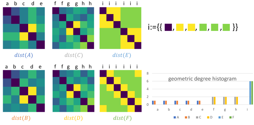
Figure 1: Distance matrices (Left) and degree histograms $d_{H}$ (Right) of three pairs of point clouds $(A,B),(C,D)$, $(E,F)$. These pairs are hard to separate by distance-based methods, as they have the same degree histogram. Nonetheless, $(A,B)$ can be separated by two iterations of 1-Geo, since $A,B\in\mathbb{R}^{3\times n}_{distinct}$. Each of $C$, $D$ is comprised of three pairs of points, each of which share the same degree. While it was shown in (Pozdnyakov & Ceriotti, 2022) that 1-Geo cannot separate $C$ from $D$, our 2-Geo can separate any distinct pair of 3D point clouds. $E$ and $F$ are especially challenging 6-dimensional point clouds in which all points have the same geometric degree.

In this section we discuss geometric graph isomorphism tests, namely, tests for checking whether two given point clouds $X,Y\in\mathbb{R}^{3\times n}$ are related by a permutation, rotation and translation (and possibly also reflection). Given two point clouds $X,Y$, these tests typically compute some feature $F(X),F(Y)$ and check whether $F(X)=F(Y)$. This feature is $\mathcal{G}$-invariant, with $\mathcal{G}$ denoting our symmetry group of choice, so that $F(X)\neq F(Y)$ automatically implies that $X\underset{\mathcal{G}}{\neq}Y$. Ideally, we would like to have complete tests, meaning that $X\underset{\mathcal{G}}{\neq}Y$ implies that $F(X)\neq F(Y)$. Typically, these require more computational resources than incomplete tests.

2.1 Incomplete geometric graph isomorphism test

Perhaps the most well-known graph isomorphism test is 1-WL. Based on this test, (Pozdnyakov & Ceriotti, 2022) formulated the following test, which we refer to as the 1-Geo test: Given two point clouds $X=(x_{1},\ldots,x_{n})$ and $Y=(y_{1},\ldots,y_{n})$ in $\mathbb{R}^{3\times n}$, this test iteratively computes for each point $x_{i}$ an $\mathcal{O}(3)$-invariant feature $h_{i}^{t}$ via

$$h_{i}^{t}=\text{{Embed}}^{(t)}\left(h_{i}^{t-1},\{\!\!\{\left(h_{j}^{t-1},\|x_{i}-x_{j}\|\right),j\neq i\}\!\!\}\right),$$ (1)

using an arbitrary initialization $h_{i}^{t}$ for $t=0$. This process is repeated $T$ times, and then a final global feature for the point cloud is computed via

$$F^{\textup{1-Geo}}(X)=\text{{Embed}}^{(T+1)}\{\!\!\{h_{i}^{T}\mid i=1,\ldots,n\}\!\!\}.$$

A similar computation is performed on $Y$ to obtain $F^{\textup{1-Geo}}(Y)$. In this test $\text{{Embed}}^{(t)}$ are hash functions, namely, they are discrete mappings of multisets to vectors, defined such that they assign distinct values to the finite number of multisets encountered during the computation of $F^{\textup{1-Geo}}$ for $X$ and $Y$. Note that by this construction, these functions are defined differently for different pairs $X,Y$.

The motivation in (Pozdnyakov & Ceriotti, 2022) in considering this test is that many distance-based symmetry-preserving networks for point clouds are in fact a realization of this test, though they use Embed functions that are continuous, defined globally on $\mathbb{R}^{3\times n}$, and in general may assign the same value to different multisets. Consequently, the separation power of these architectures is at most that of $F^{\textup{1-Geo}}$ with discrete hash functions. We note that continuous multiset functions can be used to construct architectures with the separation power of geometric isomorphism tests. This will be discussed in Section 3.

The separation power of $F^{\textup{1-Geo}}$ is closely linked to the notion of geometric degree: For a point cloud $X=(x_{1},\ldots,x_{n})$, we define the geometric degree $d(i,X)$ to be the multiset

$$d(i,X)=\{\!\!\{\|x_{1}-x_{i}\|,\ldots,\|x_{n}-x_{i}\|\}\!\!\},\quad i\in[d],$$

and the geometric degree histogram $d_{H}(X)$ to be

$$d_{H}(X)=\{\!\!\{d(1,X),\ldots,d(n,X)\}\!\!\}.$$

It is not difficult to see that if $d_{H}(X)\neq d_{H}(Y)$ then $X$ and $Y$ can be separated by $F^{\textup{1-Geo}}$ even with a single iteration $T=1$. With $T=2$, as we show in the following theorem, $F^{\textup{1-Geo}}$ can do even more, and separate $X$ and $Y$ even if $d_{H}(X)=d_{H}(Y)$, provided that the values in their histograms are all distinct, namely that $X$ and $Y$ belong to

$$\mathbb{R}^{3\times n}_{distinct}=\{X\in\mathbb{R}^{3\times n}|\,d(i,X)\neq d(j,X)\ \ \forall i\neq j\}.$$

Figure 1 depicts the distance matrices of two point clouds $A,B$ that belong to $\mathbb{R}^{3\times n}_{distinct}$ while having the same degree histogram.

Theorem 2.1.

Suppose that $X,Y\in\mathbb{R}^{3\times n}_{distinct}$, and $\text{{Embed}}^{(t)},t=1,2,3$, are multiset-to-vector functions that assign distinct values to the finite number of multi-sets encountered when computing $F^{\textup{1-Geo}}(X)$ and $F^{\textup{1-Geo}}(Y)$. Then $F^{\textup{1-Geo}}(X)=F^{\textup{1-Geo}}(Y)$ if and only if $X\underset{\mathcal{O}[3,n]}{=}Y$.

While almost any pair of point clouds $X,Y$ (in the Lebesgue sense) belongs to $\mathbb{R}^{3\times n}_{distinct}$, and thus can be separated by $F^{\textup{1-Geo}}$, this test is not complete in general. This was shown in (Pozdnyakov & Ceriotti, 2022), by providing an example of point clouds $C,D\in\mathbb{R}^{3\times 6}$ (see Figure 1)) that cannot be distinguished by $F^{\textup{1-Geo}}$.

2.2 $\mathcal{SO}[3,n]$-isomorphism test

We now describe a $2$-WL-like geometric graph isomorphism test for $\mathcal{SO}[d,n]$, which we name 2-Geo. Unlike 1-Geo, this test is complete. It is inspired by a similar test described in (Kurlin, 2022). The relationship between this work and ours is discussed in Section 7.

As a first step, we eliminate the translation symmetry by centering the point clouds $X$ and $Y$. The centering of $X=(x_{1},\ldots,x_{n})$ is the point cloud $(x_{1}^{c},\ldots,x_{n}^{c})$ defined by $x_{i}^{c}=x_{i}-\frac{1}{n}\sum_{j=1}^{n}x_{j}.$ It is known (Dym & Gortler, 2022) that the original $X$ and $Y$ are related by a symmetry in $\mathcal{SO}[3,n]$ if and only if the centralized point clouds are related by a rotation and permutation.

Now, let us make two simplifying assumptions that we shall later dispose of: (a) the first two points of $X$ and $Y$ are in correspondence- meaning that if $X$ and $Y$ can be aligned by an $\mathcal{SO}[3,n]$ transformation, then the permutation component assigns $x_{1}$ to $y_{1}$ and $x_{2}$ to $y_{2}$, and (b) the first two points in each point cloud are linearly independent.

Under these assumptions, we can define bases for $\mathbb{R}^{3}$ by $x_{1},x_{2},x_{1}\times x_{2}$ and $y_{1},y_{2},y_{1}\times y_{2}$. These two bases are related by a rotation if and only if the Gram matrices of these two bases are identical. If indeed they are, this still only implies that the first two points are related by a rotation. To check whether the remaining points are related by a rotation and permutation, it suffices to check that the unordered collection of inner products of the remaining points with the basis we defined are identical.
Formally, we define for $(i,j)=1,2$ or any other pair of indices $(i,j)$

$$X_{[i,j]} =\left[x_{i}^{c},x_{j}^{c},x_{i}^{c}\times x_{j}^{c}\right]\in\mathbb{R}^{3\times 3}$$ (2)

$$P_{[i,j,k]} =X_{[i,j]}^{T}x_{k}^{c}$$ (3)

$$G_{[i,j]}(X) =X^{T}_{[i,j]}X_{[i,j]}$$ (4)

$$h_{[i,j]}(X) =\text{{Embed}}^{(1)}\{\!\!\{P_{[i,j,k]}\,\mid\,k=3,\ldots,n\}\!\!\}$$ (5)

$$m_{[i,j]}(X) =\left(G_{[i,j]}(X),h_{[i,j]}(X)\right)$$ (6)

and we define $m_{[i,j]}(Y)$ a similar manner, where Embed is some mulitset-valued hash functions. The above construction guarantees that if $X,Y$ satisfy the simplifying assumptions (a)-(b), then $X$ and $Y$ are related by a symmetry in $\mathcal{SO}[3,n]$ if and only if $m_{[1,2]}(X)=m_{[1,2]}(Y)$.

Let us now remove the simplifying assumption (a)-(b). Since we no longer know the correspondence, instead of just considering $m_{[1,2]}$, we consider the multiset of all possible $m_{[i,j]}$ and define

$$F^{\textup{2-Geo}}(X)=\text{{Embed}}^{(2)}\{\!\!\{m_{[i,j]}(X)\,\mid\,1\leq i\neq j\leq n\}\!\!\}.$$ (7)

We define $F^{\textup{2-Geo}}(Y)$ similarly. In the appendix we prove

Theorem 2.2.

Let $X,Y\in\mathbb{R}^{3\times n}$, and let $\text{{Embed}}^{(1)},\text{{Embed}}^{(2)}$ be multiset-to-vector functions that assign distinct values to the finite number of multisets encountered when computing $F^{\textup{2-Geo}}(X)$ and $F^{\textup{2-Geo}}(Y)$. Then $F^{\textup{2-Geo}}(X)=F^{\textup{2-Geo}}(Y)$ if and only if $X\underset{\mathcal{SO}[3,n]}{=}Y$.

Proof idea

If the centralized point cloud $X^{c}$ has rank $\geq 2$, there are some $i,j$ such that $x_{i}^{c},x_{j}^{c}$ are linearly independent. If $F^{\textup{2-Geo}}(X)=F^{\textup{2-Geo}}(Y)$ then there are some $s,t$ such that $m_{[i,j]}(X)=m_{[s,t]}(Y)$, and the argument above then shows that $X\underset{\mathcal{SO}[3,n]}{=}Y$. The full proof (which does not assume any rank assumptions on $X^{c}$) is given in the appendix.

2.3 $\mathcal{O}[3,n]$-isomorphism test

The 2-Geo test described above can be modified to the scenario where reflections are also considered symmetries of the point cloud, so we would like the test to distinguish point clouds up to $\mathcal{O}[3,n]$ symmetries. A simple way to achieve this is to consider for each pair $x_{i},x_{j}$ both orientations of the vector product

$$X_{[i,j]}^{pos} =X_{i,j}=[x_{i},x_{j},x_{i}\times x_{j}]$$

$$X_{[i,j]}^{neg} =[x_{i},x_{j},-x_{i}\times x_{j}].$$

The details of this construction are given in Appendix B. Ultimately this leads to a complete $\mathcal{O}[3,n]$ test with twice the time and space complexity of the 2-Geo test for $\mathcal{SO}[3,n]$.

An interesting but less efficient alternative to the above test is to use the standard $3$-WL graph isomorphism test, with the initial label for each triplet of indices taken to be the Gram matrix corresponding to those indices. The details of this construction are described in Appendix B as well.

3 Separating Architectures

In the previous section we described incomplete and complete geometric graph isomorphism tests for $\mathcal{SO}[3,n]$ and $\mathcal{O}[3,n]$ symmetries. Our goal now is to build separating architectures based on these tests. Let us first focus on the 2-Geo test for $\mathcal{SO}[3,n]$.

To construct a separating $\mathcal{SO}[3,n]$-invariant architecture based on our 2-Geo test, we first need to choose a realization for the multiset-to-vector functions $\text{{Embed}}^{(1)}$ and $\text{{Embed}}^{(2)}$. To this end, we use parametric functions $\text{{Embed}}_{\alpha}:\mathbb{R}^{3\times(n-2)}\to\mathbb{R}^{K_{1}}$ and $\text{{Embed}}_{\beta}:\mathbb{R}^{K_{1}\times(n^{2}-n)}\to\mathbb{R}^{K_{2}}$ which are invariant to permutation of their second coordinate. Note that this also renders $F^{\textup{2-Geo}}$ parametric $F^{\textup{2-Geo}}_{\alpha,\beta}$. We will also want them to be continuous and piecewise differentiable with respect to $X,\alpha$ and $\beta$.

The main challenge is of course to guarantee that for some parameters $\alpha,\beta$, the function $F^{\textup{2-Geo}}_{\alpha,\beta}$ is $\mathcal{SO}[3,n]$ separating. A standard way (see (Anonymous, 2023; Maron et al., 2019)) to achieve this is to require that for some $\alpha,\beta$, the functions $\text{{Embed}}_{\alpha}$ and $\text{{Embed}}_{\beta}$ are injective as functions of multisets, or equivalently that they are permutation-invariant and separating. Note that by Theorem 2.2, this requirement will certainly suffice to guarantee that $F^{\textup{2-Geo}}$ is an $\mathcal{SO}[3,n]$-separating invariant. Our next step is therefore to choose permutation invariant and separating $\text{{Embed}}_{\alpha}$, $\text{{Embed}}_{\beta}$. Naturally, we will want to choose these so that the dimensions $K_{1},K_{2}$ and the complexity of computing these mappings are as small as possible.

3.1 $S_{N}$ separating invariants

We now consider the problem of finding separating invariants for the action of $S_{N}$ on $\mathbb{R}^{D\times N}$. Let us begin with the scalar case $D=1$. Two well-known separating invariant mappings in this setting are the power-sum polynomials $\Psi_{pow}$ and the sort mapping $\Psi_{sort}$, defined by

$$\Psi_{sort}(s_{1},\ldots,s_{N}) =\mathrm{sort}(s_{1},\ldots,s_{N})$$

$$\Psi_{pow}(s_{1},\ldots,s_{N}) =\left(\sum_{j=1}^{N}s_{j},\sum_{j=1}^{N}s_{j}^{2},\ldots,\sum_{j=1}^{N}s_{j}^{N}\right).$$

It is clear that $\mathrm{sort}$ is permutation-invariant and separating. It is also continuous and piecewise linear, and thus meets the regularity conditions we set out for separating invariant mappings. The power-sum polynomials are clearly smooth. Their separation can be obtained from the separation of the elementary symmetric polynomials, as discussed e.g., in (Zaheer et al., 2017).

We now turn to the case $D>1$, which is our case of interest. One natural idea is to use lexicographical sorting. However, for $D>1$, this sorting is not continuous. The power-sum polynomials can be generalized to multi-dimensional input, and these were used in the invariant learning literature (Maron et al., 2019). However, a key disadvantage is that to achieve separation, they require an extremely high embedding dimension $K=\binom{N+D}{D}$.

A more efficient approach was recently proposed in (Dym & Gortler, 2022). This method initially applies linear projections to obtain $N$ scalars and then applies a continuous $1\times N$-separating mapping $\Psi=\Psi_{pow}$ or $\Psi=\Psi_{sort}$, namely, one-dimensional power-sum polynomials or sorting. In more detail, for some natural $K$, the function $\text{{Embed}}_{\theta}:\mathbb{R}^{D\times N}\to\mathbb{R}^{K}$ is determined by a vector $\theta=(a_{1},\ldots,a_{K},b_{1},\ldots,b_{K})\in\mathbb{R}^{K(D+N)}$ where each $a_{i}$ and $b_{i}$ are $D$- and $N$-dimensional respectively, and

$$\text{{Embed}}_{\theta}(X)=\langle b_{j},\;\Psi\left(a_{j}^{T}X\right)\rangle,\;j=1,\ldots,K.$$ (8)

The following theorem shows that this mapping is permutation invariant and separating.

Theorem 3.1 ((Dym & Gortler, 2022)).

Let $\mathcal{X}$ be an $S_{N}$-invariant semi-algebraic subset of $\mathbb{R}^{D\times N}$ of dimension $D_{\mathcal{X}}$. Denote $K=2D_{\mathcal{X}}+1$. Then for Lebesgue almost every $\theta\in\mathbb{R}^{K(D+N)}$ the mapping $\text{{Embed}}_{\theta}:\mathcal{X}\to\mathbb{R}^{K}$ is $S_{N}$ invariant and separating.

When choosing $\mathcal{X}=\mathbb{R}^{D\times N}$ we get that $D_{\mathcal{X}}=N\cdot D$. The embedding dimension of $\text{{Embed}}_{\theta}$ would then be $2N\cdot D+1$. This already is a significant improvement over the cardinality of the power-sum polynomials. Another imporant point that we will soon use is that if $\mathcal{X}$ is a strict subset of $\mathbb{R}^{D\times N}$ the number of separators will depend linearly on the intrinsic dimension $D_{\mathcal{X}}$, and not on the ambient dimension $ND$.

To conclude this subsection, we note that sort-based permutation invariants such as those we obtain when choosing $\Psi=\Psi_{sort}$ are common in the invariant learning literature (Zhang et al., 2018, 2019). In contrast, polynomial-based choices such as $\Psi=\Psi_{pow}$ are not so popular. However, this choice does provide us with the following corollary.

Corollary 3.2.

Under the assumptions of the previous theorem, there exists a smooth parametric function $q_{\theta}:\mathbb{R}^{3}\to\mathbb{R}^{2D_{\mathcal{X}}+1}$ such that the separating permutation-invariant mapping $\text{{Embed}}_{\theta}:\mathbb{R}^{3\times N}\to\mathbb{R}^{2D_{\mathcal{X}}+1}$ defined using $\Psi=\Psi_{pow}$ is given by

$$\text{{Embed}}_{\theta}(x_{1},\ldots,x_{N})=\sum_{i=1}^{N}q_{\theta}(x_{i})\in\mathbb{R}^{2D_{\mathcal{X}}+1}.$$

Accordingly, in all approximation results which we will get based on the embedding $\Psi_{pow}$ we can approximate $\text{{Embed}}_{\theta}$ with a function of the form $\sum_{i=1}^{n}\mathcal{N}(x_{i})$ where $\mathcal{N}$ is a neural networks whose input and output dimension are the same as those of $\text{{Embed}}_{\theta}$.

3.2 Dimensionality of separation

From the discussion above we see that we can choose $\text{{Embed}}_{\alpha}$ to be a separating invariant mapping on $\mathbb{R}^{3\times(n-2)}$, with an embedding dimension of $K_{1}=6n-11$. It would then seem natural to choose the embedding dimension of $\text{{Embed}}_{\beta}$ so that separation on $\mathbb{R}^{K_{1}\times(n^{2}-n)}$ is guaranteed. This would require a rather high embedding dimension of $\sim n^{3}$. We note that any permutation invariant and separating mapping on $\mathbb{R}^{D\times N}$ with reasonable regularity will have embedding dimension of at least $N\cdot D$ (see (Anonymous, 2023)), and as a result we will always obtain an embedding dimension of $n^{3}$ when requiring $\text{{Embed}}_{\alpha},\text{{Embed}}_{\beta}$ to be separating on all of their (ambient) domain.

Significant savings can be obtained by the following observation: while the ambient dimension of the domain of $\text{{Embed}}_{\beta}$ is large, we only need injectivity for multisets in this domain which were obtained from some point cloud in $\mathbb{R}^{3\times n}$. Accordingly, (once $\alpha$ is fixed) $\text{{Embed}}_{\beta}$ needs only to be injective on a subset $\mathcal{X}$ of the domain whose intrinsic dimension is at most $3n$. Using Theorem 3.1 (see details in the proof of Theorem 3.4 stated below) we can take the embedding dimension of $\text{{Embed}}_{\beta}$ to be $K_{2}=6n+1$. This idea is visualized in Figure 2(a).

We note that the advantage of the intrinsic separation technique presented here is even more pronounced when considering the implementation of $F^{\textup{1-Geo}}$ with $T$ large. If we require the mappings $\text{{Embed}}^{(t)}$ to be separating and invariant on their (ambient) domain, the embedding dimension $K_{t}$ of the $t$-th mapping is at least $n+1$ times larger than the previous embedding dimension $K_{t-1}$, so that the final embedding dimension is roughly $\sim n^{T+1}$. In contrast, since the intrinsic dimension at each step is $3n$, we get a constant embedding dimension of $\sim 6n$ for all $t$, by using a variation of Theorem 3.1 for vector-multiset pairs. See Appendix E for a full explanation, and Figure 2(b) for an illustration.

3.3 Separation by feed-forward Neural Network Architectures

To summarize our discussion, the $\mathcal{SO}[3,n]$ geometric graph isomorphism discussed in Theorem 2.2 can be realized as a separating invariant architecture by replacing $\text{{Embed}}^{(1)}$ and $\text{{Embed}}^{(2)}$ with the parametric functions $\text{{Embed}}_{\alpha}$ and $\text{{Embed}}_{\beta}$ respectively as in (8), with embedding dimension $K_{1}=6n-11$ and $K_{2}=6n+1$ as discussed above, and $\Psi=\Psi_{sort}$ or $\Psi=\Psi_{pow}$. . This leads to the architecture described in Algorithm 1.

Algorithm 1 GramNet for $\mathcal{SO}[3,n]$ invariant separation

Input: $X=(x_{1},...,x_{n})\in\mathbb{R}^{3\times n}$

$X_{[i,j]}\xleftarrow[]{}\left[x_{i}^{c},x_{j}^{c},x_{i}^{c}\times x_{j}^{c}\right]$

$h_{[i,j]}(X)\xleftarrow[]{}\text{{Embed}}_{\alpha}\{\!\!\{P_{[i,j,k]},\,k\neq i,j\}\!\!\}$

$m_{[i,j]}(X)\xleftarrow[]{}\left(G_{[i,j]}(X),h_{[i,j]}(X)\right)$

$F^{\textup{2-Geo}}_{\alpha,\beta}(X)\xleftarrow[]{}\text{{Embed}}_{\beta}\{\!\!\{m_{[i,j]}(X),\quad i\neq j\}\!\!\}$

Output: $F^{\textup{2-Geo}}_{\alpha,\beta}(X)$

This result is summarized formally in the following theorem which will be proven in the appendix

Theorem 3.3.

For Lebesgue almost every $\alpha,\beta$ and $K=6n+1$, the function $F^{\textup{2-Geo}}_{\alpha,\beta}:\mathbb{R}^{3\times n}\to\mathbb{R}^{K}$ is $\mathcal{SO}[3,n]$ invariant and separating The computational complexity of evaluating $F^{\textup{2-Geo}}$ with $\Psi=\Psi_{sort}$ is $O(n^{4}\log(n))$.

We note that the same technique can be applied to convert the $\mathcal{O}[3,n]$ incomplete test $1-Geo$ and the two complete tests discussed above into separating invariant architecture.

3.4 Separation by Geometric message passing networks

The GramNet architecture proposed above is one simple example of an architecture which can achieve $\mathcal{SO}[3,n]$ separation. The basic ideas used to construct this architecture can be used to devise other separating archtiectures. As an example, we propose a modification of the well known EGNN (Victor Garcia Satorras, 2021) architecture which allows for separation. We name this architecture $\mathbf{GeoEGNN}$, and define it in Alogrithm 2

Algorithm 2 $\mathbf{GeoEGNN}$ Convolution

1:for $iteration=1,2,...,T$ do

2:     $s_{ij}\leftarrow\phi_{e}(h_{i},h_{j},m_{[i,j]})$

3:     $s_{i}\leftarrow\text{{Embed}}_{\beta}\{\!\!\{s_{i1},...,s_{in}\}\!\!\}$

4:     $h_{i}\leftarrow\phi_{\epsilon}(s_{i},h_{i})$

5:end for

6:$h_{global}=\text{{Embed}}_{\gamma}\{\!\!\{h_{1},\ldots,h_{n}\}\!\!\}$

The main change we made in EGNN to obtain separation is the replacement of the simple invariant feature $|x_{i}-x_{j}|$ with the significantly more expressive edge feature: $m_{[i,j]}(X)$ defined in Algorithm 1. In EGNN the functions $\phi_{e},\phi_{\epsilon}$ are typically taken to be neural networks and the Embed functions are just sums. This is ‘asymptotically separating’ according to Corollary 3.2. To achieve full separation we take $\text{{Embed}}_{\beta},\text{{Embed}}_{\gamma}$ as in Equation 8, and claim

Theorem 3.4.

For almost every $\alpha,\beta,\gamma$, $\mathbf{GeoEGNN}$ is an $\mathcal{SO}[3,n]$-Invariant Separator with embedding dimension of $6n+1$.

Proof idea

After a single convolution, each hidden state, $h_{i}$, is an embedding of $\{\!\!\{m_{[i,j]}|i\neq j,1\leq j\leq n\}\!\!\}$. The output after decoding will be an embedding of $\{\!\!\{h_{1},...,h_{n}\}\!\!\}$. Intuitively, this embedding has more information than the mere unordered list of $\{\!\!\{m_{[i,j]}|1\leq i,j\leq n\}\!\!\}$, and thus separation can be derived from Theorem 2.2.

4 From Separation to Universality

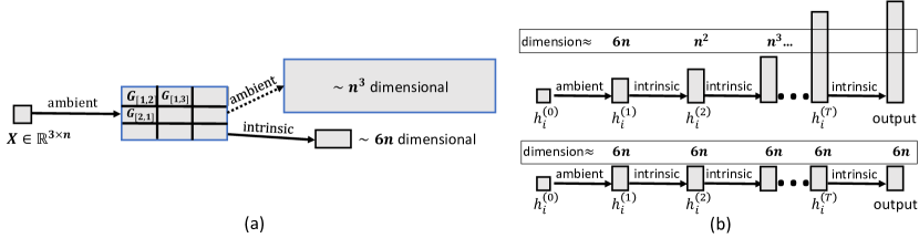
Figure 2: The standard method for constructing architectures that are equivalent to isomorphism tests uses injective multiset mappings on the ambient domain. The embedding dimension of such mapping increases exponentially with depth. In contrast, Theorem 3.1 allows for injective multiset functions whose dimensionality is twice the intrinsic dimension of the features which is always $3n$. The figure shows the implementation of these two approaches for the computation of $F^{\textup{2-Geo}}$ and $F^{\textup{1-Geo}}$.

ccccccccc Point Clouds GramNet GeoEGNN EGNN LinearEGNN MACE TFN DimeNet GVPGNN
Hard1[2] 1.0 0.998 0.5 1.0 1.0 0.5 1.0 1.0
Hard2 [2] 1.0 0.97 0.5 1.0 1.0 0.5 1.0 1.0
Hard3 [2] 1.0 0.85 0.5 1.0 1.0 0.55 1.0 1.0
Harder [1] 1.0 0.899 0.5 0.5 1.0 0.5 1.0 1.0
Cholesky dim=6 1.0 Irrelevant 0.5 0.5 1.0 Irrelevant Irrelevant Irrelevant
Cholesky dim=8 1.0 Irrelevant 0.5 0.5 1.0 Irrelevant Irrelevant Irrelevant
Cholesky dim=12 N/A Irrelevant 0.5 0.5 0.5 Irrelevant Irrelevant Irrelevant

Table 1: Results of our models on challenging point clouds [1] (Pozdnyakov & Ceriotti, 2022) [2] (Pozdnyakov et al., 2020) Fig. S4

In the previous section we described several models that are invariant and separating with respect to the action of $\mathcal{SO}[3,n]$ and $\mathcal{O}[3,n]$. We shall now discuss how these models can be used to achieve universality. A standard argument (e.g., (Villar et al., 2021)), is that invariant functions can always be approximated by compositions of separating functions with fully connected neural networks.

Theorem 4.1 (Separation implies universality).

Let $f:\mathbb{R}^{d\times n}\to\mathbb{R}$ be a continuous invariant function w.r.t. $\mathcal{O}[d,n]$ (or $\mathcal{SO}[d,n]$). Let $F:\mathbb{R}^{d\times n}\to\mathbb{R}^{K}$ be a continuous separating invariant. Then for any compact set $M\subseteq\mathbb{R}^{d\times n}$ and $\epsilon>0$ there exists a neural network $\mathcal{N}$ such that $$|f(x)-\mathcal{N}\circ F(x)|\leq\epsilon,\forall x\in M.$$ It follows from Theorem 4.1 that a composition of $\mathbf{GramNet}$ or $\mathbf{GeoEGNN}$ with a fully connected neural networks can approximate any continuous invariant functions on $M$. Note that the conditions of the theorem are satisfied when using the power-sum polynomials or sorting function as realizations of $\text{{Embed}}_{\alpha},\text{{Embed}}_{\beta}$. By Corollary 3.2, universality can also be obtained using embeddings of the form $\sum_{i=1}^{n}\mathcal{N}(x_{i})$, with $\mathcal{N}$ being a neural network.

4.1 Universality for Rotation-Equivariant models

Separating invariants are useful not only for proving universality of invariant models, but also for equivariant models. In our context, we use a result from (Villar et al., 2021) which showed that a permutation invariant and $\mathcal{O}(3)$ equivariant functions can be written as combinations of general invariant functions and simple equivariant functions. Since this result requires $\mathcal{O}(3)$ invariance, we use a modification of Algorithm 2 to $\mathcal{O}(3)$ invariance which is described formally in the appendix in Algorithm 3. We then obtain the following equivariant universality result:

Theorem 4.2 (Equivariant Universality).

Let $f:\mathbb{R}^{3\times n}\to\mathbb{R}^{3}$ be continuous, $\mathcal{O}(3)$-equivariant and translation and permutation invariant. Then for any compact $M\subset\mathbb{R}^{3\times n}$ and any $\varepsilon>0$, $f$ can be approximated to $\epsilon$-accuracy uniformly on $M$ by functions of the form

$$\tilde{f}(X)=\sum_{k=1}^{n}\mathcal{N}(h_{k},h_{global})x_{k}^{c},$$

where $h_{k}(X),h_{global}(X)$ are the output of Algorithm 3 and $\mathcal{N}$ is a fully connected neural network.

ccccccccccccc Property $\alpha$ $\varepsilon_{HOMO}$ $H$ $\varepsilon_{LUMO}$ $\Delta\varepsilon$ $\mu$ $C_{\nu}$ $G$ $R^{2}$ $U$ $U_{0}$ $ZPVE$
$\left[units\right]$ $bohr^{3}$ meV meV meV meV D cal/mol K meV $bohr^{3}$ meV meV meV
EGNN 0.073 29 12 25 48 0.029 0.031 12 0.106 12 11 1.55
GeoEGNN 0.068 27.9 11.6 38.3 45.8 0.032 0.031 10.75 0.1004 11.5 10.5 1.61

Table 2: Results on QM9 Dataset

5 Experiments

5.1 Separation experiment

To evaluate the separation power of different architectures, we constructed a dataset consisting of pairs of point clouds that are particularly difficult to separate. This dataset will be made available for public use.

Each pair of point clouds $X_{1},X_{2}$ is used as a prototype, from which we generate data samples for a binary classification task. Samples are generated by randomly choosing one of ${X_{1},X_{2}}$, applying a random rotation and permutation to it and adding noise. The task is to determine whether each sample originates from $X_{1}$ or $X_{2}$.

We used the following challenging pairs: (i) Hard1-Hard3: Three pairs of 3D point clouds from (Pozdnyakov et al., 2020). In each pair, both clouds have the same degree histogram, but are members of the set $\mathbb{R}^{3\times n}_{distinct}$ — which can be separated by 1-Geo according to Theorem 2.1. The distance matrices for one such pair are visualized in $A,B$ of Figure 1.  (ii) Harder: A pair of 3D point clouds from (Pozdnyakov & Ceriotti, 2022) that are not in $\mathbb{R}^{3\times n}_{distinct}$, and provably cannot be separated by 1-Geo. These are $C,D$ in Figure 1.  (iii) Cholesky dim=d: Pairs $X_{1},X_{2}$ of $d$ points in $\mathbb{R}^{d}$, with $d=6,8,12$. All points in $X_{1}$, $X_{2}$ have the same degree histogram. The point clouds $E,F$ for $d=6$ appear in Figure 1. Further details appear in Appendix A.

The results appear in Section 4. First, as our theory predicts, $\mathbf{GramNet}$ achieves perfect separation on all examples, while in the $0.1$ noise level we use $\mathbf{GeoEGNN}$ to achieve good but not perfect separation.

Next, note that EGNN (Victor Garcia Satorras, 2021) fails for all examples. Surprisingly, replacing the neural networks in EGNN with simple linear functions (LinearEGNN) does yield successful separation of examples in $\mathbb{R}^{3\times n}_{distinct}$, as predicted in Theorem 2.1.

Finally, note that Tensor Field Networks (Thomas et al., 2018) does not separate our examples well, while MACE (Batatia et al., ), DimeNet (Gasteiger et al., 2020) and GVPGNN (Jing et al., ) do. Of these methods, only MACE is applicable to problems with $d>3$, and it has failed to separate for the $d=12$ case. GramNet was unable to run for $d=12$ due to memory constraints.

5.2 Invariant regression on QM9

We evaluated our architectures on the QM9 Dataset for molecular property prediction (Ramakrishnan et al., 2014). To implement GeoEGNN we used the original implementation of EGNN (Victor Garcia Satorras, 2021) augmented by the addition of our $h_{[i,j]}$ of Equation 5 as edge features. As shown in Section 4.1, this minor modification of EGNN typically leads to improved results. In contrast, despite its excellent separation properties GramNet is not competitive on this task.

6 Conclusion

We presented fully separating architectures whose embedding dimension depends linearly on the point cloud’s dimension, in stark contrast to contemporary approaches with an exponential dependence. Our implementation of these architectures achieves good separation results in practice and yields improved results in several tasks on the QM9 benchmark. We believe these results will open the door to further improvements, both in the theoretical understanding of what is necessary for separation and in the development of separating architectures with good practical performance.

7 Related Work

WL equivalence. The relationship between the $k$-WL test and GNNs is very well-studied. Proofs of equivalence of GNNs and $k$-WL often assume a countable domain (Xu et al., 2018) or require separation only for a single graph (Morris et al., 2018). To the best of our knowledge, our separation result is the first one in which, for a fixed parameter vector (and in fact for almost all such vectors), separation is guaranteed for all graphs with features in a continuous domain. This type of separation could be obtained using the power-sum methodology in (Maron et al., 2019), but the complexity of this construction is exponentially worse than ours (see Subsections 3.1 and 3.2).

Complete Invariants and universality. As mentioned earlier, several works describe $\mathcal{SO}[3,n]$ and $\mathcal{O}[3,n]$ equivariant point-cloud architectures that are universal. However, these rely on high-dimensional representations of $SO(d)$ (Dym & Maron, 2020; Finkelshtein et al., 2022; Gasteiger et al., 2021) or $S_{n}$ (Lim et al., 2022).

In the planar case $d=2$, universality using low-dimensional features was achieved in (Bökman et al., 2022). For general $d$, a complete test similar to our 2-Geo was proposed in (Kurlin, 2022). However, it uses Gram-Schmidt orthogonalization, which leads to discontinuities at point clouds with linearly-dependent points. Moreover, the complete invariant features defined there are not vectors, but rather sets of sets. As a result, measuring invariant distances for $d=3$ requires $O(n^{7.5}+n^{3.5}log^{3}(n))$ arithmetic operations, whereas using GramNet invariant features only requires $O(n^{4}log(n))$ operations. Finally, we note that more efficient tests for equivalence of geometric graphs were suggested in (Brass & Knauer, 2000), but there does not seem to be a straightforward way to modify these constructions to efficiently compute a complete, continuous invariant feature.

Weaker notions of universality

We showed that 1-Geo is complete on the subset $\mathbb{R}^{3\times n}_{distinct}$. Similar results for a simpler algorithm, and with additional restrictions, were obtained in (Widdowson & Kurlin, 2022). Efficient separation/universality can also be obtained for point clouds with distinct principal axes (Puny et al., 2021; Kurlin, 2022), or when only considering permutation (Qi et al., 2017) or rigid (Wang et al., 2022) symmetries, rather than considering both symmetries simultaneously.

Acknowledgements

N.D. acknowledges the support of the Horev Fellowship.

Appendix A Experiments: additional details

A.1 Separation experiment-creating the Cholesky examples

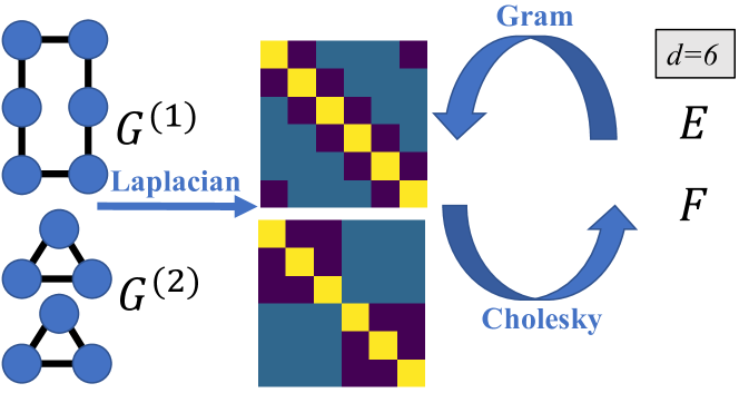
Figure 3: Creation of difficult-to-separate point clouds from difficult-to-separate graphs.

Figure 1 shows the distance matrices of two point clouds $E,F\in\mathbb{R}^{6\times 6}$ where all points in both $E$ and $F$ have the same geometric degree. The way this example was created is illustrated in Figure 3. We chose two non-isomorphic 2-regular graphs $G^{(1)}$ and $G^{(2)}$ with six vertices. This pair is a classical example of non-isomorphic graphs not distinguished by standard 1-WL. We consider the Laplacians of the two graphs. Note that up to reordering, the columns of the Laplacian are all the same, as we would like the columns of our distance matrices to be. Since the two Laplacians $L^{(1)},L^{(2)}$ are positive semi-definite, we can take their Cholesky decomposition and obtain two matrices $E,F\in\mathbb{R}^{6\times 6}$ satisfying $E^{T}E=L^{(1)}$ and $F^{T}F=L^{(2)}$. Thus, $L^{(1)}$ and $L^{(2)}$, which as we said have the structure we desire, are the Gram matrices of $E$, so that the columns $e_{1},\ldots,e_{6}$ of $E$ satisfy

$$\langle e_{i},e_{j}\rangle=L^{(1)}_{ij}$$

Since

$$\|e_{i}-e_{j}\|^{2}=\langle e_{i},e_{i}\rangle-2\langle e_{i},e_{j}\rangle+\langle e_{j},e_{j}\rangle$$

we see that the distance matrix of $E$ (and $F$) has the desired structure as well.

This technique for generating hard-to-separate point clouds from hard-to-separate graphs was used to generate the three examples ‘Cholesky dim=6’, ‘Cholesky dim=8’ and ‘Cholesky dim=12’ in Table 4, wherein all three cases the graphs we considered were on $2N$ vertices, one of the graphs consisted of two disjoint cycles of size $N$ and the other graph consisted of a single cycle of size $2N$.

A.2 Separation experiment-additional details

We modified code by (Anonymous, 2023) for testing the performance of various contemporary invariant learning models. We augmented their binary classification method, which included training on replicas of a pair of point clouds and then testing on the same pair, by introducing random noise, permutations, and rotations in each training and testing iteration.
We used a dataset size of 100,000 instances, although most models converged prior to the end of training. Then we used validation and test sets of 1000 samples. We added Gaussian-distributed noise with mean zero and variance of 0.1, for all of our experiments. For applying rotations we used the geometric learning library geotorch, all other implementations were primarily in PyTorch 1.13.1.

Our implementation of GeoEGNN uses sort-based embeddings. We found that it obtains better results when the parameters of the embedding are generated randomly and not learned. The output of the embedding is fed into a fully-connected neural network with learned parameters. LinearEGNN is identical to the original EGNN algorithm (with equivariant coordinate updates) yet rather than neural network functions we simply used linear projections.

A.3 QM9 Experiment

Dataset description. The QM9 Dataset is a benchmark dataset for geometric graph models. It is a quantum chemistry dataset of the chemical space of small organic molecules. The molecules vary in size, ranging from 3 to 29 atoms per molecule. Apart from the geometric information, each atom is decorated with its Atomic number, also known as its z-value. The chemical interaction of atoms is dependent on their z-values. It comprises a total of about 130,000 such samples. The targets are various continuous molecular properties, such as Lowest Unoccupied Molecular Orbit. Molecules are naturally invariant to translations, rotations, and permutations, which makes this regression task fitting for invariant learning models.

Implementation Details. As mentioned in the main text, we implemented GeoEGNN for QM9 by taking the original EGNN model endowed with additional low-dimensional edge features $h_{[i,j]}$. In the architecture, we used two-layer Neural Networks for $\phi_{e}$ a single-layer NN for $\phi_{\epsilon}$, both of width 150. For embedding $\{\!\!\{P_{[i,j]}\;|\;i\neq j\}\!\!\}$ we used an embedding dimension of 1. As a side note, the intrinsic space is of dimension 2$\cdot$3$\cdot$29 + 1 = 175, yet in practice, this embedding dimension was too computationally constraining. To account for the molecules’ varying sizes we implemented the approach by (Zhang et al., 2019), which uses a linear interpolation of the weights.

The results in Section 4.1 are an average over three independent parameter initialization per task. To account for the possibility that these improvements are merely due to optimization of parameter tuning rather than the improved approximation capability, we tested optimization schemes, including using the same Neural Network width as GeoEGNN, and did not improve upon EGNN’s results on the QM9 dataset as reported in their original paper (Victor Garcia Satorras, 2021).

We implemented the code in PyTorch v1.13.1. We used batch size of 96 for all property targets with changing learning rate, depending on the property. We used Adam Optimizer for weight regularization and Cosine Annealing-based learning rate scheduler. We ran our experiments on a single NVIDIA A40 GPU, with an average of 350 epochs which required an average of 24 hours to complete.

Appendix B $\mathcal{O}[3,n]$ separation

B.1 $2$-WL like $\mathcal{O}[3,n]$ isomorphism test

In this appendix we describe two $\mathcal{O}[3,n]$ complete geometric isomorphism tests. In our first, more efficient construction we define $m^{pos}_{[i,j]}=m_{[i,j]}$ and define $m^{neg}_{[i,j]}$ by applying the same process described in the main text to achieve $m_{[i,j]}$, but when

$$X_{[i,j]}^{pos}=X_{i,j}=[x_{i},x_{j},x_{i}\times x_{j}]$$

is replaced by

$$X_{[i,j]}^{neg}\coloneqq[x_{i},x_{j},x_{j}\times x_{i}].$$

We then define

$$F^{\mathrm{reflect}}(X)=\text{{Embed}}^{(2)}\left[\{\!\!\{m^{pos}_{[i,j]},m^{neg}_{[i,j]}\;:\;i\neq j\}\!\!\}\right]$$

The following theorem, proven in Appendix C, shows that this test is complete:

Theorem B.1.

Assume that $X,Y\in\mathbb{R}^{3\times n}$, and $\text{{Embed}}^{(1)},\text{{Embed}}^{(2)}$ are multiset-to-vector functions which assign distinct values to the finite number of multi-sets encountered when computing $F^{\mathrm{reflect}}(X)$ and $F^{\mathrm{reflect}}(Y)$. Then $F^{\mathrm{reflect}}(X)=F^{\mathrm{reflect}}(Y)$ if and only if $X\underset{\mathcal{O}[3,n]}{=}Y$.

B.2 $3$-WL based $\mathcal{O}[3,n]$ isomorphism test

We now describe a construction of separating invariants for the $\mathcal{O}[3,n]$ action which relies only on inner products. While this construction is $n$ times more expensive then the previous construction, we bring it here as it is useful in order to analyze the many $\mathcal{SO}[3,n]$ equivariant methods which rely only on inner products, such as (Victor Garcia Satorras, 2021). Additionally this geometric graph isomorphism test can be fully realized as a $3$-WL test.

For a given $X=(x_{1},\ldots,x_{n})\in\mathbb{R}^{3\times n}$, and a given triplet $\mathbf{i}=(i_{1},i_{2},i_{3})\in[n]^{3}$, we define an initial (continuous) label $\mathbf{C}^{(0)}(\mathbf{i})(X)$ to be the $3\times 3$ Gram matrix consisting of all inner products of the points $x_{i_{1}},x_{i_{2}},x_{i_{3}}$. We then apply the standard $3$-WL test (which is sometimes called the Folkore 3-WL test, e.g., in (Maron et al., 2019)). Namely, given a labeling for every triplet $\mathbf{i}$ at time $t-1$, we define a new labeling at time $t$ by

$$\mathbf{D}^{(t)}_{j}(\mathbf{i}) =\left(\mathbf{C}^{(t-1)}(j,i_{2},i_{3}),\mathbf{C}^{(t-1)}(i_{1},j,i_{3}),\mathbf{C}^{(t-1)}(i_{1},i_{2},j)\right)$$

$$\mathbf{C}^{(t)}(\mathbf{i}) =\left(\mathbf{C}^{(t-1)}(\mathbf{i}),\text{{Embed}}^{(t)}\{\!\!\{\mathbf{D}^{(t)}_{j}(\mathbf{i}),j\in[n]\}\!\!\}\right)$$

This operation is repeated $T$ times, and the final labeling is used to compute a global label $\mathbf{C}(X)$ to the point cloud via

$$\mathbf{C}(X)=\text{{Embed}}\{\!\!\{\mathbf{C}^{(T)}(\mathbf{i}),\mathbf{i}\in[n]^{3}\}\!\!\}.$$

Our claim in Theorem B.2 (which we prove in Appendix C) is that this procedure is complete even when $T=1$:

Theorem B.2.

For every $X,Y\in\mathbb{R}^{3\times n}$, a single iteration of the $3$-WL test with initial coloring of $3\times 3$ Gram matrices as defined above, fails to separate $X$ from $Y$ if and only if $X\underset{\mathcal{O}[3,n]}{=}Y$.

Appendix C Proofs

Remark C.1.

Throughout the proofs we will implicitly use the fact that original $X,Y\in\mathbb{R}^{d\times n}$ are related by a symmetry in $\mathcal{SO}[d,n]$ (or $\mathcal{O}[d,n]$) if and only if the centralized point clouds are related by a rotation (and reflection) and permutation. Additionally, we note that the translation operation is translation invariant, and equivariant with respect to permutations, and multiplication from the left by a rotation, reflection, or any other matrix. Thus, in all the proof we will in practice assume that $X,Y$ are already centralized and only discuss invariance and separation with respect to $\mathcal{SO}(d)\times S_{n}$ (or $O(d)\times S_{n}$).

See 2.1

Proof.

By the invariance of $F^{\textup{1-Geo}}$, if $X\underset{\mathcal{O}[3,n]}{=}Y$ then $F^{\textup{1-Geo}}(X)=F^{\textup{1-Geo}}(Y)$. In the other direction, assume that $X,Y\in\mathbb{R}^{3\times n}_{distinct}$ and $X\underset{\mathcal{O}[3,n]}{\neq}Y$. We need to show that $F^{\textup{1-Geo}}(X)\neq F^{\textup{1-Geo}}(Y)$. We first note that since $X,Y\in\mathbb{R}^{3\times n}_{distinct}$ we have that

$$h_{i}^{1}(X)\neq h_{j}^{1}(X)\text{ and }h_{i}^{1}(Y)\neq h_{j}^{1}(Y),\forall i\neq j.$$

We now consider two possible options: in the first option, we assume that there is some $i$ such that $h_{i}^{1}(X)\neq h_{j}^{1}(Y)$ for all $j=1,\ldots,n$. In this situation we will have the same inequality $h_{i}^{2}(X)\neq h_{j}^{2}(Y)$ for all $j=1,\ldots,n$ also when $t=2$ and therefore $F^{\textup{1-Geo}}(X)\neq F^{\textup{1-Geo}}(Y)$.

If the first option does not occur, then there exists a permutation $\tau$ such that $h_{i}^{1}(X)=h_{\tau(i)}^{1}(Y)$ for all $i=1,\ldots,n$. If such a permutation exists it is unique. For simplicity of notation we assume without loss of generality that $\tau$ is the identity permutation so that $h_{i}^{1}(X)=h_{i}^{1}(Y)$. Since by assumption $X\underset{\mathcal{O}[3,n]}{\neq}Y$, there must be some $i,j$ such that $\|x_{i}-x_{j}\|\neq\|y_{i}-y_{j}\|$. For this $i$, note that for all $k=1,\ldots,n$ with $k\neq i$ we have that

$$(h_{j}^{1}(X),\|x_{i}-x_{j}\|)\neq(h_{k}^{1}(Y),\|y_{i}-y_{k}\|)$$

for $k=j$ this is because the second coordinate is different, and for $k\neq j$ this is because the first coordinate is different. It follows that

$$h_{i}^{2}(X)\neq h_{i}^{2}(Y).$$

Since $h_{i}^{1}(X)\neq h_{j}^{1}(Y)$ for all $j\neq i$ we have that $h_{i}^{2}(X)\neq h_{j}^{2}(Y)$ in this case as well. It follows that $F^{\textup{1-Geo}}(X)\neq F^{\textup{1-Geo}}(Y)$. ∎

See 2.2

Proof.

Let X, Y $\in\mathbb{R}^{3\times n}$. By Definition 1.1, we need to prove invariance and separation of $F^{\textup{2-Geo}}$, with respect to $\mathcal{SO}[d,n]$, to prove this theorem. Using Remark C.1 we only need to really consider separation and invariance with respect to $\mathcal{SO}(3)\times S_{n}$ and we don’t neet to ‘worry about’ translations.

Separation:

Assume $F^{\textup{2-Geo}}(X)=F^{\textup{2-Geo}}(Y)$.
Define r = $\underset{i\neq j}{\max}$ $\operatorname{rank}(G_{[i,j]})$. By assumption we have $\{\!\!\{G_{[i,j]}(X)|i\neq j\}\!\!\}=\{\!\!\{G_{[i,j]}(Y)|i\neq j\}\!\!\}$ , thus $r(X)=r(Y)$ and there exist $i,j,s,t\in[n]$ such that $G_{[i,j]}=G_{[s,t]}$ ($\star$) and they both have rank $r$.
By (Kraft & Procesi, 1996), the equality of Gram matrices implies that there exists an orthogonal transformation, $T\in\mathcal{O}(3)$, such that

$$T(x_{i})=y_{s},\;T(x_{j})=y_{t},\;T(x_{i}\times x_{j})=y_{s}\times y_{t}.$$ (9)

If $x_{i}\times x_{s}\neq 0$ we see that $T$ preserves orientation and therefore $T\in\mathcal{SO}(3)$. If not, and if $T$ is a reflection, we can modify $T$ to be a rotation which still satisfies (9) by composing it with a relfection that fixes the $\leq 1$ dimensional subspace spanned by $x_{i},x_{j}$. Thus in any case we can assume that $T\in\mathcal{SO}(3)$. By assumption and ($\star$), we have $\{\!\!\{P_{[i,j,k]}(X)\,k\neq i,j\}\!\!\}=\{\!\!\{P_{[s,t,k]}(Y),\,k\neq i,j\}\!\!\}$.
This implies that there exists some permutation $\sigma\in S_{n}$ such that $\sigma(i)=s.\sigma(j)=t$ and for all $k=1,\ldots,n$

$$\langle y_{s},Tx_{k}\rangle=\langle Tx_{i},Tx_{k}\rangle=\langle x_{i},x_{k}\rangle=\langle y_{s},y_{\sigma(k)}\rangle$$

and similarly

$$\langle y_{t},Tx_{k}\rangle =\langle y_{t},y_{\sigma(k)}\rangle$$

$$\langle y_{s}\times y_{t},Tx_{k}\rangle =\langle y_{s}\times y_{t},y_{\sigma(k)}\rangle$$

Now note that each $y_{k}$ is in the span of $y_{s},y_{t},y_{s}\times y_{t}$ (even when $r<3$), and similarly every $x_{k}$ is in the span of $x_{s},x_{t},x_{s}\times x_{t}$ and so $Tx_{k}$ is also in the span of $y_{s},y_{t},y_{s}\times y_{t}$. It follows that $Tx_{k}-y_{\sigma(k)}=0$, and thus we showed that $X$ and $Y$ are related by a $\mathcal{SO}(3)\times S_{n}$ transformation.

Invariance:

Let $X\in\mathbb{R}^{d\times n}$.
We first show that if $\sigma\in S_{n}$ then $F^{\textup{2-Geo}}(X)=F^{\textup{2-Geo}}(\sigma X)$. Note that

$$G_{[i,j]}(\sigma X)=G_{[\sigma^{-1}(i),\sigma^{-1}(j)]}(X),\,h_{[i,j]}(\sigma X)=h_{[\sigma^{-1}(i),\sigma^{-1}(j)]}(X),m_{[i,j]}(\sigma X)=m_{[\sigma^{-1}(i),\sigma^{-1}(j)]}(X)$$

and therefore

$$\{\!\!\{m_{[i,j]}(X)|i\neq j\}\!\!\}=\{\!\!\{m_{[i,j]}(\sigma X)|i\neq j\}\!\!\}$$

Thus we have shown permutation invariance.
If $S\in\mathcal{SO}(3)$. Then $F^{\textup{2-Geo}}(X)=F^{\textup{2-Geo}}(SX)$ follows from the $\mathcal{SO}(3)$ invariance of inner products and the $\mathcal{SO}(3)$ equivariance of vector products. ∎ See B.1

Proof.

Proof is almost identical to that of Theorem 2.2, up to considering both orientations of the perpendicular vector (cross product vector).
$F^{\mathrm{reflect}}$ is defined as:

$$F^{\mathrm{reflect}}(X)=\text{{Embed}}^{(2)}\{\!\!\{m^{pos}_{[i,j]},m^{neg}_{[i,j]}\;:\;i\neq j\}\!\!\}$$

Let $X,Y\in\mathbb{R}^{3\times n}$.
By Definition 1.1, we need to prove invariance and separation of $F^{\mathrm{reflect}}$, with respect to $\mathcal{O}[3,n]$, to prove this theorem.

Separation:

Define r = $\underset{i\neq j}{\max}$ $\operatorname{rank}(G_{[i,j]})$.
By assumption we have $\{\!\!\{G_{[i,j]}(X)\}\!\!\}=\{\!\!\{G_{[i,j]}(Y)\}\!\!\}$ , thus $r(X)=r(Y)$ and there exists a 4-tuple $(i,j,s,t)\in[n]^{4}$ such that $G^{b^{\prime}}_{[s,t]}=G^{b}_{[i,j]}$ for $b,b^{\prime}\in\{pos,neg\}$.
By (Kraft & Procesi, 1996), there exists a unique Orthogonal transformation $T\in O(3)$, such that

$$T(x_{i})=y_{s},\>T(x_{j})=y_{t},\>T(x_{i}\times x_{j})=y_{s}\times y_{t}$$

or

$$T(x_{i})=y_{s},\>T(x_{j})=y_{t},\>T(x_{i}\times x_{j})=\mathbf{-}y_{s}\times y_{t}.$$

Arguing as in the proof of the previous theorem, we see that $X$ and $Y$ are related by $T\in\mathcal{O}(3)$ and an appropriate permutation

Invariance

: This argument too is similar to the argument in the previous theorem.

∎ See B.2

Proof.

As in the previous proofs we assume our point clouds are centered so we don’t need to worry about translations. The invariance of the construction to permutations and $\mathcal{O}(3)$ transformations is rather straightforward, we focus on showing separation.

Assume we are given $X,Y\in\mathbb{R}^{3\times n}$ such that after a single iteration $T=1$ of the $3$-WL algorithm

$$\mathbf{C}(X)=\mathbf{C}(Y)$$

which implies that

$$\{\!\!\{\mathbf{C}^{(1)}(\mathbf{i})(X),\mathbf{i}\in[n]^{3}\}\!\!\}=\{\!\!\{\mathbf{C}^{(1)}(\mathbf{i})(Y),\mathbf{i}\in[n]^{3}\}\!\!\}$$

It follows that $X$ and $Y$ have the same rank $r$, and there exists some $\mathbf{i}=(i_{1},i_{2},i_{3})$ and $\mathbf{i}^{\prime}$, both with distinct indices

$$i_{1}\neq i_{2},i_{2}\neq i_{3},i_{3}\neq i_{1},$$

such that $\mathbf{C}^{(1)}(\mathbf{i})(X)=\mathbf{C}^{(1)}(\mathbf{i}^{\prime})(Y)$ and $\mathbf{C}^{(0)}(\mathbf{i})(X)$ and $\mathbf{C}^{(0)}(\mathbf{i}^{\prime})(Y)$ both are Gram matrices of rank $r$. It follows that there is some $T\in\mathcal{O}(3)$ taking the $\mathbf{i}$ indices of $X$ to the $\mathbf{i}^{\prime}$ indices of $Y$. Additionally, since $\mathbf{C}^{(1)}(\mathbf{i})(X)=\mathbf{C}^{(1)}(\mathbf{i}^{\prime})(Y)$ we also have that there is some permutation $\tau\in S_{n}$ which takes $\mathbf{i}$ to $\mathbf{i}^{\prime}$. and so that

$$D_{j}^{(0)}(\mathbf{i})(X)=D_{\tau(j)}^{(0)}(\mathbf{i}^{\prime})(Y).$$

This implies that the inner products of $y_{\tau(j)}$ with the $\mathbf{i}^{\prime}$ indices of $Y$ are the same as the inner products of $x_{j}$ with the $\mathbf{i}$ indices of $X$, and since the points at these indices span the whose space spanned by $Y$ and $X$ respectively it follows that $X$ and $Y$ are related by the orthogonal transformation $T$ and their permutation $\tau$ (see previous theorems for a detailed description of this argument).

∎

See 3.3

Proof.

By Theorem 2.2 it is sufficient to show that for Lebesgue almost every $(\alpha,\beta)$, the mapping $\text{{Embed}}_{\alpha}$ is permutation invariant and separating on $\mathbb{R}^{3\times n}$, and the mapping $\text{{Embed}}_{\beta}$ is permutation invariant and separating on the image of the mapping $f_{\alpha}$ which we define as

$$f_{\alpha}(X)=\left(m_{[i,j]}(X),i\neq j\right).$$

By Theorem 3.1 we know that $\text{{Embed}}_{\alpha}$ is separating for Lebesgue almost every $\alpha$. For fixed $\alpha$, we know that $f_{\alpha}$ is a semi-algebraic mapping as a composition of semi-algebraic mappings, and therefore the dimension of its image is $\leq\dim(\mathbb{R}^{3\times n})=3n$ (see (Basu et al., 2006) for the necessary real algebraic geometry statements re composition and dimension). To apply Theorem 2.2 we need to work with a permutation invariant domain, so we require $f_{\alpha}$ to be injective on

$$\bigcup_{\sigma\in S_{n^{2}-n}}\sigma(f_{\alpha}(\mathbb{R}^{3\times n}))$$

which is a finite union of sets of dimension $\leq 3n$ and hence also has dimension $\leq 3n$. It follows that for almost every $\beta$ the function $\text{{Embed}}_{\beta}$ is separating on this permutation invariant set. Using Fubini’s theorem, this implies that for almost every $(\alpha,\beta)$ the functions $\text{{Embed}}_{\alpha}$ and $\text{{Embed}}_{\beta}$ are both separating, and this proves the theorem.

We conclude by discussing the complexity of computing $F^{\textup{2-Geo}}$. Calculating each $m_{i,j}$ using sort-based embeddings $\text{{Embed}}_{\alpha}$ requires $\mathcal{O}(n^{2}\log(n))$ operations. Since there are $\mathcal{O}(n^{2})$ such $m_{[i,j]}$ the total complexity of computing all of them is $\mathcal{O}(n^{4}\log(n))$. In the second step we compute $\text{{Embed}}_{\beta}$ on multisets of size $D\times N$ where $D=\mathcal{O}(n),N=\mathcal{O}(n^{2})$, and with embedding dimension of $\mathcal{O}(n)$. This requires $\mathcal{O}(n^{4}+n^{3}\log(n))$ operations , so the total complexity is $\mathcal{O}(n^{4}\log(n))$

We can naturally extend this result to arbitrary $d$, and get complexity of $\mathcal{O}(n^{d+1}\log(n))$ (where we consider the limit $n\rightarrow\infty$ with $d$ fixed).

∎

See 3.4

Proof.

As in the proof of Theorem 3.3, we can show that for almost every $\alpha,\beta,\gamma$ the functions $\text{{Embed}}_{\alpha}.\text{{Embed}}_{\beta},\text{{Embed}}_{\gamma}$ are separating on their respective (intrinsic) domains.

After a single iteration we have the following embeddings:

$$h_{i}=\text{{Embed}}_{\beta}\{\!\!\{m_{[i,j]}\;|\;i\neq j\}\!\!\}$$

$$h_{global}=\text{{Embed}}_{\gamma}\{\!\!\{h_{i}\;|\;i\in[n]\}\!\!\}$$

In particular, if $h_{global}(X)=h_{global}(Y)$ for $X,Y\in\mathbb{R}^{3\times n}$ then

$$\{\!\!\{\{\!\!\{m_{[i,j]}(X)|i\neq j\}\!\!\}\;|\;i\in[n]\}\!\!\}=\{\!\!\{\{\!\!\{m_{[i,j]}(Y)|i\neq j\}\!\!\}\;|\;i\in[n]\}\!\!\}\implies\{\!\!\{m_{[i,j]}(X)|i\neq j\}\!\!\}=\{\!\!\{m_{[i,j]}(Y)|i\neq j\}\!\!\}$$

Then , by Theorem 2.2, we have that

$$X\underset{\mathcal{SO}[3,n]}{=}Y$$

. Thus $h_{global}$ is an $\mathcal{SO}[3,n]$ Invariant Separator. As explained in Section 3.2, the dimension of $\text{{Embed}}_{\gamma}$ need only be 2$\dim(\mathcal{X})$ +1, which for the case of 3D Geometric Graphs is $\dim(\mathcal{X})=3n$. Then, it is sufficient for $h_{global}$ to be of dimension 6n+1 to guarantee separation.

∎

See 4.1

Proof.

Let $\epsilon>0$ and $M\subseteq\mathbb{R}^{d\times n}$ a compact set. Using Proposition 1.3 in (Dym & Gortler, 2022), there exists a continuous $f^{\epsilon}$ such that

$$|f(x)-f^{\epsilon}\circ F(x)|<\frac{\epsilon}{2}$$

The image of a a compact set under a continuous function is a compact set, see (Munkres, 2000), then $S\coloneqq\operatorname{Im}{(F)}$ is compact. By the Universal Approximation Theorem (Cybenko, 1989; Pinkus, 1999), we can approximate $f^{\epsilon}$ with a fully-connected Neural Network with arbitrary precision, i.e. there exists a Neural Network Function $f^{FC}$ such that for all $x\in S$,

$$|f^{\epsilon}(x)-f^{FC}(x)|<\frac{\epsilon}{2}$$

By the Triangle Inequality, for all $x\in M$,

$$|f(x)-f^{FC}\circ F(x)|\leq|f(x)-f^{\epsilon}\circ F(x)|+|f^{\epsilon}\circ F(x)-f^{FC}\circ F(x)|<\frac{\epsilon}{2}+\frac{\epsilon}{2}=\epsilon$$

∎

See 4.2

Proof.

We first modify GeoEGNN to obtain $\mathcal{O}[3,n]$ invariance and separation.

Algorithm 3 GeoEGNN Convolution for $\mathcal{O}[3,n]$

1:for $iteration=1,2,...,T$ do

2:     $s_{ij}\leftarrow\phi_{e}(h_{i},h_{j},m_{[i,j]}^{pos},m_{[i,j]}^{neg})$

3:     $s_{i}\leftarrow\text{{Embed}}_{\beta}\{\!\!\{s_{i1},...,s_{in}\}\!\!\}$

4:     $h_{i}\leftarrow\phi_{\epsilon}(s_{i},h_{i})$

5:end for

6:$h_{global}=\text{{Embed}}_{\gamma}\{\!\!\{h_{1},\ldots,h_{n}\}\!\!\}$

First, analogously to the proof of Theorem 3.4, we can show that GeoEGNN for $\mathcal{O}[3,n]$ is an $\mathcal{O}[3,n]$ Invariant Separator.
Our argument for asality is based on Proposition 10 in (Villar et al., 2021):

Proposition C.2.

(Villar et al., 2021) Let $g:\mathbb{R}^{d\times n}\to\mathbb{R}^{d}$   be $\mathcal{O}$(d) equivariant and also permutation-invariant. Then $g$ can be written as

$$g(x_{1},...,x_{n})=\sum_{k=1}^{n}f(x_{k},x_{1},...,x_{k-1},x_{k+1},...,x_{n})x_{k}$$ (10)

where $f$ is invariant to $O(d)$ and permutations of the last $n-1$ inputs.

We first note that $g$ is additionally translation invariant (as we assume) if and only if

$$g(x_{1},...,x_{n})=\sum_{k=1}^{n}f(x_{k}^{c},x_{1}^{c},...,x_{k-1}^{c},x_{k+1}^{c},...,x_{n}^{c})x_{k}^{c}$$ (11)

Accordingly, our goal is to show that for every $k$ we can approximate $f(x_{k}^{c},x_{1}^{c},...,x_{k-1}^{c},x_{k+1}^{c},...,x_{n}^{c})$ arbitrarily well by $\mathcal{N}(h_{k},h_{global})$ on compact sets. This can be accomplished using Theorem 4.1, once we show that $X\to(h_{k},h_{global})$ is an invariant separator for actions of $\mathcal{O}(3)\times Stab(k)$, where $Stab(k)$ is the subgroup of permutation in $S_{n}$ which keep $k$ fixed. The invariance of this mapping is rather straightforward. We now show separation.Let $(h_{k},h_{global}),(h^{\prime}_{k},h^{\prime}_{global})$ be outputs of a $\mathcal{O}[3,n]$ $\mathbf{GeoEGNN}$ convolution for point clouds X, Y, respectively. due to $\mathcal{O}[3,n]$ separation we have that

$$h_{global}=h^{\prime}_{global}\implies X\underset{\mathcal{O}(3)\times S_{n}}{=}Y\;\;(\star\star)$$

So $X$ and $Y$ are related by some permutation $\sigma$ and some $T\in\mathcal{O}(3)$. Note that $h_{k}=h_{k}^{\prime}$ implies in particular that $\|x_{k}\|=\|y_{k}\|$ and thus $x_{k}=0$ if and only if $y_{k}=0$. In this case we can choose the permutation $\sigma$ so that $\sigma(k)=k$. Now let us assume that $x_{k},y_{k}$ are both non-zero. We have that

$$h_{k}=h^{\prime}_{k}\implies\{\!\!\{m_{[k,j]}^{o}(X)|\;k\neq j,\;o\in\{neg,pos\}\}\!\!\}=\{\!\!\{m_{[k,j]}^{o}(Y)|\;k\neq j,\;o\in\{neg,pos\}\}\!\!\}.$$

Since $x_{k}$ is non-zero, it can be completed by some indices $\ell\neq k$ so that $x_{k},x_{\ell},x_{k}\times x_{\ell}$ is a basis for the span of $x_{1},\ldots,x_{k}$. We then have that $m_{[k,j]}^{pos}(X)=m_{[k,\ell]}^{o}(Y)$ for some $\ell\neq j$ and some $o\in\{pos,neg\}$. It follows from arguments we have seen in the proof of Theorem 2.2 that $X,Y$ are related by an orthogonal transformation and a permutation that takes $k$ to $k$ (and $j$ to $\ell$).

∎

Appendix D Algorithms for general $d$

Here we explain our algorithms for general $d$.

D.1 Generalization of Cross Product

The complete 2-Geo test for $d=3$ point clouds can be generalized to a $(d-1)$-Geo test for general $d$ point clouds. $F^{\textup{(d-1)-Geo}}$ is defined as

$$F^{\textup{(d-1)-Geo}}(X)=\text{{Embed}}^{(2)}\{\!\!\{\left(G_{[\mathbf{i}]}(X),\text{{Embed}}^{(1)}\{\!\!\{P_{[\mathbf{i},k]}(X),\,k\notin\mathbf{i}\}\!\!\}\right),\mathbf{i}\in[n]^{d-1}\}\!\!\}$$

where for for a tuple $\mathbf{i}\in[n]^{d-1}$, we define $G_{[\mathbf{i}]}\coloneqq X_{\mathbf{i}}^{T}X_{\mathbf{i}}$ for $X_{\mathbf{i}}=\left[x_{i_{1}},\ldots,x_{i_{d-1}},x_{\mathbf{i}}^{\star}\right]$ where

$$x_{\mathbf{i}}^{\star}=\mathbf{Plucker}((x_{i_{1}}\land\ldots\land x_{i_{d-1}})^{\star})$$

where $(\cdot)^{\star}$ is the Hodge Star operator and Plucker is the Plucker embedding.
Letting V =$span\{x_{i_{1}},\ldots,x_{i_{d-1}}\}$ We note that through the Plucker embedding the Hodge star operator can be seen as a mapping $V\to V^{\perp}$ taking the oriented basis of V, $\{x_{i_{1}},\ldots,x_{i_{d-1}}\}$ to an oriented basis of $V^{\perp}=span\{x_{\mathbf{i}}^{\star}\}$, (Flanders et al., 1963; Harris, 2010). For d=3 these definitions coincide with those in proof of Theorem 2.2.
The Hodge star operator is defined uniquely up to orientation and completes a basis for d-1 linearly independent vectors. Replacing the cross product with the Hodge star operator naturally extends our proof of Theorem 2.2 to the d-dimensional case. The $\mathcal{O}[d,n]$ tests we suggest can be generalized to $\mathcal{O}[d,n]$ tests in a similar fashion.

D.2 Computational Complexity

The computation of the Hodge star operator is of order O($d^{4}$) which is not substantial in the setting where $n\gg d$. Thus analogously to explanation in Theorem 3.3, we obtain an order of O($n^{d+1}\log(n)$) arithmetic operations for computing $F^{\textup{(d-1)-geo}}$.

Appendix E extension to vector-multiset pairs

Our construction of architectures with efficient continuous multiset embeddings was based on Theorem E.1. To apply a similar technique to $1-Geo$ and specifically to (1) where we define the update rule

$$h_{i}^{t}=\text{{Embed}}^{(t)}\left(h_{i}^{t-1},\{\!\!\{\left(h_{j}^{t-1},\|x_{i}-x_{j}\|\right),j\neq i\}\!\!\}\right),$$

we need a version of this theorem that can handle vector-multiset pairs. This is a simple extension of the previous theorem. Say our input is a pair $(h,X)$, where $h\in\mathbb{R}^{F}$ is a vector and $X\in\mathbb{R}^{D\times N}$ represents the multiset: we choose a vector-muliset embedding

$$\text{{Embed}}_{\omega}(h,X)=\langle c_{j},h\rangle+\langle b_{j},\;\Psi\left(a_{j}^{T}X\right)\rangle,\;j=1,\ldots,K.$$ (12)

where $\omega=(a_{1},\ldots,a_{K},b_{1},\ldots,b_{K},c_{1},\ldots,c_{K})\in\mathbb{R}^{K(F+D+N)}$ and $\Psi=\Psi_{pow}$ or $\Psi=\Psi_{sort}$. We then claim

Theorem E.1.

Let $\mathcal{X}$ be an semi-algebraic subset of $\mathbb{R}^{F}\oplus\mathbb{R}^{D\times N}$ of dimension $D_{\mathcal{X}}$, which is invariant to the action of $S_{N}$ on $\mathbb{R}^{D\times N}$. Denote $K=2D_{\mathcal{X}}+1$. Then for Lebesgue almost every $\omega\in\mathbb{R}^{K(D+N)}$ the mapping $\text{{Embed}}_{\omega}(h,X):\mathbb{R}^{F}\oplus\mathbb{R}^{D\times N}\to\mathbb{R}^{K}$ is a separating invariant mapping with respect to the action of $S_{N}$ on $\mathcal{X}$.

Idea of proof

Using the main theorem in (Dym & Gortler, 2022), it is sufficient to show that for every fixed pair $(h,X)$ and $(h^{\prime},X^{\prime})$ which are not related by an $S_{N}$ symmetry, ‘most’ choices of parameters in (12) will separate $(h,X)$ from $(h^{\prime},X^{\prime})$, or more accurately, that the set of parameter vectors $(a,b,c)$ failing to do so is not full-dimensional, that is

$$\dim\{(a,b,c)|\quad\langle c,h\rangle+\langle b,\;\Psi\left(a^{T}X\right)\rangle=\langle c,h^{\prime}\rangle+\langle b,\;\Psi\left(a^{T}X^{\prime}\right)\rangle\}<F+D+N.$$ (13)

If $(h,X)$ and $(h^{\prime},X^{\prime})$ are not related by symmetry, this means that either $h\neq h^{\prime}$ or $X$ and $X^{\prime}$ are not related by an $S_{N}$ symmetry. In the latter case, Proposition 2.1 in (Dym & Gortler, 2022) shows that for ‘most’ $a,b$

$$\langle b,\;\Psi\left(a^{T}X\right)\rangle\neq\langle b,\;\Psi\left(a^{T}X^{\prime}\right)\rangle$$ (14)

Thus, for ‘most’ $a,b$ either (14) holds or $h\neq h^{\prime}$ (or both occur). when this occurs, ‘most‘ $c$ do not satisfy the equation

$$\langle c,h\rangle+\langle b,\;\Psi\left(a^{T}X\right)\rangle=\langle c,h^{\prime}\rangle+\langle b,\;\Psi\left(a^{T}X^{\prime}\right)\rangle$$

as the $c$ satisfying this linear equation are a strict subspace of the domain $\mathbb{R}^{F}$ of $c$. Thus overall we see that ‘most’ $a,b,c$ do separate $(h,X)$ from $(h^{\prime},X^{\prime})$.

Turning this argument into a full formal proof involves replacing the intuitive notion of ‘most’ used here with the formal definition in (13). This can be done using Lemma 1.10 in (Dym & Gortler, 2022).

References

- Anonymous (2023) Anonymous. On the expressive power of geometric graph neural networks. In Submitted to The Eleventh International Conference on Learning Representations, 2023. URL https://openreview.net/forum?id=Rkxj1GXn9_. under review.
- Basu et al. (2006) Basu, S., Pollack, R., and Roy, M.-F. Algorithms in Real Algebraic Geometry. Springer Berlin, Heidelberg, 2006. ISBN 978-3-540-33098-1.
- (3) Batatia, I., Kovacs, D. P., Simm, G. N., Ortner, C., and Csanyi, G. Mace: Higher order equivariant message passing neural networks for fast and accurate force fields. In Advances in Neural Information Processing Systems.
- Bökman et al. (2022) Bökman, G., Kahl, F., and Flinth, A. Zz-net: A universal rotation equivariant architecture for 2d point clouds. In Proceedings of the IEEE/CVF Conference on Computer Vision and Pattern Recognition, pp. 10976–10985, 2022.
- Brass & Knauer (2000) Brass, P. and Knauer, C. Testing the congruence of d-dimensional point sets. In Proceedings of the sixteenth annual symposium on Computational geometry, pp. 310–314, 2000.
- Chen et al. (2019) Chen, Z., Villar, S., Chen, L., and Bruna, J. On the equivalence between graph isomorphism testing and function approximation with gnns. Advances in neural information processing systems, 32, 2019.
- Cybenko (1989) Cybenko, G. Approximation by superpositions of a sigmoidal function. Mathematics of control, signals and systems, 2(4):303–314, 1989.
- Deng et al. (2021) Deng, C., Litany, O., Duan, Y., Poulenard, A., Tagliasacchi, A., and Guibas, L. J. Vector neurons: A general framework for so (3)-equivariant networks. In Proceedings of the IEEE/CVF International Conference on Computer Vision, pp. 12200–12209, 2021.
- Dym & Gortler (2022) Dym, N. and Gortler, S. J. Low dimensional invariant embeddings for universal geometric learning. arXiv preprint arXiv:2205.02956, 2022.
- Dym & Maron (2020) Dym, N. and Maron, H. On the universality of rotation equivariant point cloud networks. arXiv preprint arXiv:2010.02449, 2020.
- Finkelshtein et al. (2022) Finkelshtein, B., Baskin, C., Maron, H., and Dym, N. A simple and universal rotation equivariant point-cloud network. arXiv preprint arXiv:2203.01216, 2022.
- Flanders et al. (1963) Flanders, H., Publications, D., and Collection, K. M. R. Differential Forms with Applications to the Physical Sciences. Dover books on advanced mathematics. Academic Press, 1963. ISBN 9780486661698. URL https://books.google.co.il/books?id=9PdQAAAAMAAJ.
- Gasteiger et al. (2020) Gasteiger, J., Groß, J., and Günnemann, S. Directional message passing for molecular graphs. arXiv preprint arXiv:2003.03123, 2020.
- Gasteiger et al. (2021) Gasteiger, J., Becker, F., and Günnemann, S. Gemnet: Universal directional graph neural networks for molecules, 2021. URL https://arxiv.org/abs/2106.08903.
- Harris (2010) Harris, J. Algebraic Geometry: A First Course. Graduate Texts in Mathematics. Springer New York, 2010. ISBN 9781441930996. URL https://books.google.co.il/books?id=kq8HkgAACAAJ.
- (16) Jing, B., Eismann, S., Suriana, P., Townshend, R. J. L., and Dror, R. Learning from protein structure with geometric vector perceptrons. In International Conference on Learning Representations.
- Kondor (2018) Kondor, R. N-body networks: a covariant hierarchical neural network architecture for learning atomic potentials. arXiv preprint arXiv:1803.01588, 2018.
- Kraft & Procesi (1996) Kraft, H. and Procesi, C. Classical invariant theory: a primer. 1996.
- Kurlin (2022) Kurlin, V. Computable complete invariants for finite clouds of unlabeled points under euclidean isometry, 2022. URL https://arxiv.org/abs/2207.08502.
- Lim et al. (2022) Lim, D., Robinson, J., Zhao, L., Smidt, T., Sra, S., Maron, H., and Jegelka, S. Sign and basis invariant networks for spectral graph representation learning. arXiv preprint arXiv:2202.13013, 2022.
- Maron et al. (2019) Maron, H., Ben-Hamu, H., Serviansky, H., and Lipman, Y. Provably powerful graph networks. In Wallach, H., Larochelle, H., Beygelzimer, A., d'Alché-Buc, F., Fox, E., and Garnett, R. (eds.), Advances in Neural Information Processing Systems, volume 32. Curran Associates, Inc., 2019. URL https://proceedings.neurips.cc/paper/2019/file/bb04af0f7ecaee4aae62035497da1387-Paper.pdf.
- Morris et al. (2018) Morris, C., Ritzert, M., Fey, M., Hamilton, W. L., Lenssen, J. E., Rattan, G., and Grohe, M. Weisfeiler and leman go neural: Higher-order graph neural networks. ArXiv, abs/1810.02244, 2018.
- Munkres (2000) Munkres, J. Topology. Featured Titles for Topology. Prentice Hall, Incorporated, 2000. ISBN 9780131816299. URL https://books.google.co.il/books?id=XjoZAQAAIAAJ.
- Pinkus (1999) Pinkus, A. Approximation theory of the mlp model in neural networks. Acta Numerica, 8:143 – 195, 1999.
- Pozdnyakov & Ceriotti (2022) Pozdnyakov, S. and Ceriotti, M. Incompleteness of graph convolutional neural networks for points clouds in three dimensions. 01 2022. URL arXiv:2201.07136v4.
- Pozdnyakov et al. (2020) Pozdnyakov, S. N., Willatt, M. J., Bartók, A. P., Ortner, C., Csányi, G., and Ceriotti, M. Incompleteness of atomic structure representations. Phys. Rev. Lett., 125:166001, Oct 2020. doi: 10.1103/PhysRevLett.125.166001. URL https://link.aps.org/doi/10.1103/PhysRevLett.125.166001.
- Puny et al. (2021) Puny, O., Atzmon, M., Smith, E. J., Misra, I., Grover, A., Ben-Hamu, H., and Lipman, Y. Frame averaging for invariant and equivariant network design. In International Conference on Learning Representations, 2021.
- Qi et al. (2017) Qi, C. R., Su, H., Mo, K., and Guibas, L. J. Pointnet: Deep learning on point sets for 3d classification and segmentation. In Proceedings of the IEEE conference on computer vision and pattern recognition, pp. 652–660, 2017.
- Ramakrishnan et al. (2014) Ramakrishnan, R., Dral, P. O., Rupp, M., and Von Lilienfeld, O. A. Quantum chemistry structures and properties of 134 kilo molecules. Scientific data, 1(1):1–7, 2014.
- Thomas et al. (2018) Thomas, N., Smidt, T., Kearnes, S., Yang, L., Li, L., Kohlhoff, K., and Riley, P. Tensor field networks: Rotation-and translation-equivariant neural networks for 3d point clouds. arXiv preprint arXiv:1802.08219, 2018.
- Victor Garcia Satorras (2021) Victor Garcia Satorras, E. H. M. W. E(n) equivariant graph neural networks. Proceedings of the 38-th International Conference on Machine Learning, PMLR(139), 2021.
- Villar et al. (2021) Villar, S., Hogg, D. W., Storey-Fisher, K., Yao, W., and Blum-Smith, B. Scalars are universal: Equivariant machine learning, structured like classical physics, 2021. URL https://arxiv.org/abs/2106.06610.
- Wang et al. (2022) Wang, L., Liu, Y., Lin, Y.-C., bin Liu, H., and Ji, S. Comenet: Towards complete and efficient message passing for 3d molecular graphs. ArXiv, abs/2206.08515, 2022.
- Widdowson & Kurlin (2022) Widdowson, D. and Kurlin, V. Resolving the data ambiguity for periodic crystals. In Advances in Neural Information Processing Systems, 2022.
- Xu et al. (2018) Xu, K., Hu, W., Leskovec, J., and Jegelka, S. How powerful are graph neural networks? ArXiv, abs/1810.00826, 2018.
- Zaheer et al. (2017) Zaheer, M., Kottur, S., Ravanbakhsh, S., Poczos, B., Salakhutdinov, R. R., and Smola, A. J. Deep sets. Advances in neural information processing systems, 30, 2017.
- Zhang et al. (2018) Zhang, M., Cui, Z., Neumann, M., and Chen, Y. An end-to-end deep learning architecture for graph classification. In Proceedings of the AAAI conference on artificial intelligence, volume 32, 2018.
- Zhang et al. (2019) Zhang, Y., Hare, J., and Prügel-Bennett, A. Fspool: Learning set representations with featurewise sort pooling. arXiv preprint arXiv:1906.02795, 2019.