Armouring of a frictional interface by mechanical noise

Abstract

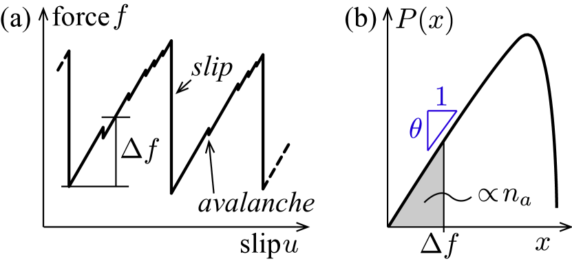
A dry frictional interface loaded in shear often displays stick-slip. The amplitude of this cycle depends on the probability that a slip event nucleates into a rupture, and on the rate at which slip events are triggered. This rate is determined by the distribution $P(x)$ of soft spots which yields if the shear stress is increased by some amount $x$. In minimal models of a frictional interface that include disorder, inertia and long-range elasticity, we discovered an ‘armouring’ mechanism, by which the interface is greatly stabilised after a large slip event: $P(x)$ then vanishes at small arguments, as $P(x)\sim x^{\theta}$ de Geus et al. (2019). The exponent $\theta>0$, which exists only in the presence of inertia (otherwise $\theta=0$), was found to depend on the statistics of the disorder in the model, a phenomenon that was not explained. Here, we show that a single-particle toy model with inertia and disorder captures the existence of a non-trivial exponent $\theta>0$, which we can analytically relate to the statistics of the disorder.

1 Introduction

We study systems in which disorder and elasticity compete, leading to intermittent, avalanche-type response under loading. Examples include an elastic line being pulled over a disordered pinning potential, or frictional interfaces  Fisher (1998); Narayan and Fisher (1993); Kardar (1998). When subject to an external load $f$, such systems are pinned by disorder when the load is below a critical value $f_{c}$. At $f>f_{c}$, the system moves forward at a finite rate. At $f=f_{c}$ the system displays a crackling-type response described by avalanches whose sizes and durations are distributed according to powerlaws.

A key aspect of such systems is the distribution of soft spots Müller and Wyart (2015). If we define $x$ as the force increase needed to trigger an instability locally, then increasing the remotely applied force by $\Delta f$ will trigger $n_{a}\propto\int_{0}^{\Delta f}P(x)dx$ avalanches, with $P(x)$ the probability density of $x$. The relevant behaviour of $P(x)$ therefore is that at small $x$. Let us assume that $P(x)\sim x^{\theta}$ at small $x$, such that $n_{a}\propto(\Delta f)^{\theta+1}$.

Classical models used to study the depinning transition consider an over-damped dynamics Fisher (1998). In that case, it can be shown that $\theta=0$ Fisher (1998). This result is not true for certain phenomena, including the plasticity of amorphous solids or mean-field spin glasses. In these cases, due to the fact that elastic interactions are long-range and can vary in sign (which is not the case for the depinning transition, where a region that is plastically rearranged can only destabilise other regions), one can prove that $\theta>0$, as reviewed in Müller and Wyart (2015); Rosso et al. (2022).

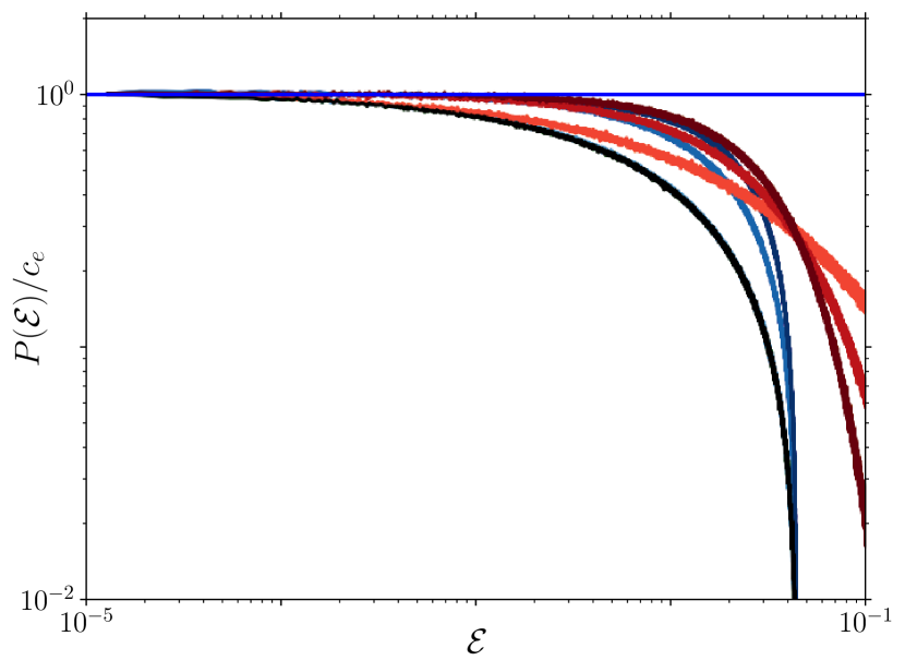
Recently, we studied simple models of dry frictional interface de Geus et al. (2019); de Geus and Wyart (2022). We considered disorder, long-range elastic interactions along the interface. These interactions are strictly positive as in the usual class of the depinning transition. However, we studied the role of inertia, that turns out to have dramatic effects. Inertia causes transient overshoots and undershoots of the stress resulting from a local plastic event. It thus generates a mechanical noise, that lasts until damping ultimately takes place. Remarkably, we found that right after system-spanning slip events, $\theta>0$ de Geus et al. (2019) in the presence of inertia. Intuitively, such an ‘armouring’ mechanism results from the mechanical noise stemming inertial effects, that destabilises spots close to an instability (i.e. small $x$), thus depleting $P(x)$ at small argument. This property is consequential: the number of avalanches of plastic events triggered after a system-spanning rupture is very small. As a consequence, the interface can increase its load when driven quasistatically in a finite system, without much danger of triggering large slip events. The interface therefore present larger stick-slip cycles due to this effect, as sketched in Fig. 1. Thus, one of the central quantities governing the stick-slip amplitude is $\theta$ de Geus et al. (2019).

Our previous model de Geus et al. (2019) divided the interface in blocks whose mechanical response was given by a potential energy landscape that, as a function of slip, comprised a sequence of parabolic wells with equal curvature. We drew the widths $w$ of each well randomly from a Weibull distribution, such that its distribution $P_{w}(w)\sim w^{k}$ at small $k$. We empirically found $\theta\simeq 2.5$ for $k=1$ and $\theta\simeq 1.4$ for $k=0.2$.

Here we present a toy model for a region of space that stops moving at the end of a large slip event. In the most idealised view, we describe this region as a single particle that moves over a disordered potential energy landscape, and that slows down due to dissipation. We model this potential energy landscape by a sequence of parabolic potentials that have equal curvature $\kappa$ but different widths taken from $P_{w}(w)$, with $w$ the width of a parabola. In this model, $x=\kappa w/2$ and is thus proportional to the width of the well in which the particle stops. Below we prove that for such a model, $P(x)\sim x^{k+2}$ if $P_{w}(w)\sim w^{k}$. This result explains both why $\theta>0$ and why this exponent in non-universal, as it depends on $k$ that characterises the disorder. Although this prediction does not match quantitatively our previous observations, the agreement is already noticeable for such a simple model. We support our argument with analytical proofs, and verify our conclusion numerically. The generality of our argument suggests that the presence of a non-trivial exponent $\theta$ may hold in other depinning systems, as long a inertia is present.

(a)

(b)

Figure 1: (a) Sketch of stick-slip response: “slip” events punctuate periods in which the interface is macroscopically stuck, but microscopic events (“avalanches”) do occur. The number of avalanches $n_{a}\propto(\Delta f)^{\theta+1}$, which can be linked to (b) the distribution of soft spots. $x$ is thereby the amount of force needed to trigger an instability locally. Right after a large slip event, its distribution empirically scales like $P(x)\sim x^{\theta}$ at small $x$ as indicated (log-scale implied).

2 Model

During a big slip event, all regions in space are moving but eventually slow down and stop. We model this by considering a single region in space in which a particle of finite mass is thrown into the potential energy landscape at a finite velocity. In the simplest case, this particle is “free”, such that it experiences no external driving and stops due to dissipation, see Fig. 2. This corresponds to the Prandtl-Tomlinson Prandtl (1928); Tomlinson (1929); Popov and Gray (2014) model that describes the dynamics of one (driven) particle in a potential energy landscape. The equation of motion of the “free” particle reads

$$m\ddot{r}=f_{e}(r)-\eta\dot{r}.$$ (1)

with $r$ the particle’s position, $m$ its mass, and $\eta$ a damping coefficient. $f_{e}(r)$ is the restoring force due to the potential energy landscape. We consider a potential energy landscape that consists of a sequence of finite-sized, symmetric, quadratic wells, such that the potential energy inside a well $i$ is given by $U(r)=(\kappa/2)(r-r_{\min}^{i})^{2}+U_{0}^{i}$ for $r_{\mathrm{y}}^{i}<r\leq r_{\mathrm{y}}^{i+1}$, with $w_{i}\equiv r_{\mathrm{y}}^{i+1}-r_{\mathrm{y}}^{i}$ the width of the well, $\kappa$ the elastic constant, $r_{\min}^{i}\equiv(r_{\mathrm{y}}^{i}+r_{\mathrm{y}}^{i+1})/2$ the position of the center of the well, and $U_{0}^{i}=\kappa(w^{i})^{2}/8$ an unimportant offset. The elastic force deriving from this potential energy is $f_{e}(r)\equiv-\partial_{x}U(r)=\kappa(r_{\min}^{i}-r)$. With $\kappa$ is constant, the landscape is parameterised by the distance between two subsequent cusps $w_{i}$, which we assume identically distributed (iid) according to a distribution $P_{w}(w)$. We consider underdamped dynamics corresponding to $\eta^{2}<4m\kappa$. Within a well, the dynamics is simply that of a underdamped oscillator, as recalled in Appendix A.

Figure 2: Evolution of the kinetic energy $E$ as a function of position $r$ (in red) of the “free” particle ‘thrown’ into a potential energy landscape (shown in the inset). Every entry into a new well is indicated using a marker. A thin green line shows the evolution of the total energy (with the definition of the inset, it has the local minimum of the last well as arbitrary offset).

3 Stopping well

Distribution

We are interested in the width of the well in which the particle eventually stops. Suppose that a particle enters a well of width $w$ with a kinetic energy $\mathcal{E}$. The particle stops in that well if $\mathcal{E}<E_{c}(w)$, with $E_{c}$ the minimum kinetic energy with which the particle needs to enter a well of width $w$ to be able to exit. The distribution of wells in which particles stop in that case is

$$P_{s}(w)\sim P_{w}(w)P(\mathcal{E}<E_{c}(w)),$$ (2)

with $P_{w}(w)$ the probability density of well widths, and $P_{s}(w)$ the probability of well widths in which the particle stops. Within one well, the particle is simply a damped harmonic oscillator as has been studied abundantly. In the limit of a weakly damped system, the amount of kinetic energy lost during one cycle is $\Delta E=\kappa w^{2}(1-\exp(-2\pi/Q))/8$ with the quality factor $Q=\sqrt{4m\kappa/\eta^{2}-1}$. The minimal kinetic energy with which the particle needs to enter the well in order to be able to exist is thus $E_{c}=\Delta E\propto w^{2}$ (see Appendix B for the exact calculation of $E_{c}$). Furthermore, if $P(\mathcal{E})$ is a constant at small argument (as we will argue below), then

$$P(\mathcal{E}<E_{c}(w))=\int_{0}^{E_{c}}P(\mathcal{E})\mathrm{d}\mathcal{E}\sim E_{c}(w).$$ (3)

Therefore, the particle stops in a well whose width is distributed as

$$P_{s}(w)\sim w^{2}P_{w}(w).$$ (4)

Central result

Once stopped, the force, $x$, by which we need to tilt the well in which the particle stopped, in order for it to exit again is $x=\kappa w/2$ , such that our central result is that

$$P(x)\sim x^{2}P_{w}(x).$$ (5)

For example, if $P_{w}(w)\sim w^{k}$ at small $w$, we predict that

$$P(x)\sim x^{2+k}.$$ (6)

Energy at entry

We will now argue that the density of kinetic energy with which the particle enters the final well, $P(\mathcal{E})$, is finite at small $\mathcal{E}$. For one realisation, $\mathcal{E}$ results from passing many wells with random widths. If its kinetic energy is much larger than the potential energy of the typical wells, it will not stop. We thus consider that the particle energy has decreased up to some typical kinetic energy $E_{0}$ of the order of the typical potential energy $\kappa\langle w^{2}\rangle/8$. If the particle exits the next well, at exit it will have a kinetic energy $\mathcal{K}=E_{0}-\Delta E(E_{0},w)$. For a given $E_{0}$ and distributed $w$, we have:

$$P(\mathcal{E})=\int dw\,P_{w}(w)\,\delta(\mathcal{K}(E_{0},w)-\mathcal{E}).$$ (7)

It thus implies that:

$$P(\mathcal{E}=0)=P_{w}(w^{*})/\left|\partial_{w}\mathcal{K}\big{|}_{w=w^{*}}\right.$$ (8)

$w^{*}$ is the well width for which the particle reaches the end of the well with zero velocity, i.e. $E_{0}=E_{c}(w^{*})$. By assumption, $P_{w}(w^{*})>0$. Furthermore we prove in Appendix C that $\partial_{w}\mathcal{K}|_{w=w^{*}}=\kappa w^{*}/2>0$. Overall, it implies that $P(\mathcal{E}=0)>0$, i.e. $P(\mathcal{E})$ does not vanish as $E\rightarrow 0$, from which our conclusions follow.

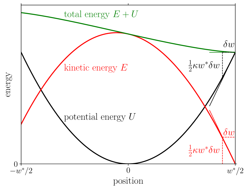
Here we give a simple argument for $\partial_{w}\mathcal{K}|_{w=w^{*}}=\kappa w^{*}/2>0$. Given $E_{0}$, but an infinitesimally smaller well of width $w^{*}-\delta w$, the particle will enter the next well. Because the velocity is negligible in the vicinity of $w^{*}$, the damping is negligible. Therefore, $\delta\mathcal{K}$ is of the order of the difference in potential energy on a scale $\delta w$, $\delta U=U(w^{*})-U(w^{*}-\delta w)\approx\kappa w^{*}\delta w/2$, as we illustrate in Fig. 3. We thus find that $\partial_{w}\mathcal{K}|_{w=w^{*}}=\lim_{\delta w\rightarrow 0}\delta K/\delta w=\kappa w^{*}/2$.

Figure 3: Evolution of the kinetic energy $E$ (red), potential energy $U$ (black), and total energy $E+V$ (green) for a particle that has entered a well of width $w^{*}$ with a kinetic energy $E_{0}=E_{c}(w^{*})$ such that it stops just. Consequently, $\partial_{r}(E+V)|_{w^{*}/2}=0$, which can be decomposed in $\partial_{r}V|_{w^{*}/2}=\kappa w^{*}/2$ such that $\partial_{r}E|_{w^{*}/2}=-\kappa w^{*}/2$, as indicated using thin lines.

4 Numerical support

Objective

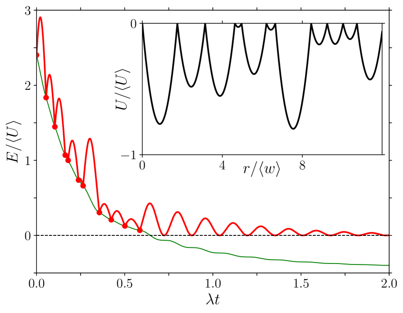
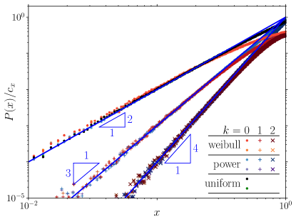
We now numerically verify our prediction that $P(x)\sim x^{k+2}$ (Eq. 6). We simulate a large number of realisations of a potential energy landscape constructed from randomly drawn widths (considering different distributions $P_{w}(w)$) and constant curvature. We study the distribution of stopping wells if a “free” particle is ‘thrown’ into the landscape at a high initial velocity (much larger than $v_{c}(\langle w\rangle)$ such that particle transverses many wells before stopping).

Map

We find an analytical solution for Eq. 1 in the form of a map. In particular, we derive the evolution of the position in a well based on an initial position $-w/2$ and velocity in Appendix A. This maps the velocity with which the particle enters a well at position $w/2$, to an exit velocity which corresponds to the entry velocity of the next well, etc.

Stopping well

We record the width of the stopping well, $x$, and the velocity $\mathcal{V}$ with which the particle enters the final well. We find clear evidence for the scaling $P(x)\sim x^{k+2}$ in Fig. 4. Perturbing the evolution with random force kicks changes nothing to our observations, as included in Fig. 4 (see caption). We, furthermore, show that the probability density of the kinetic energy with which the particle enters the final well, $P(\mathcal{E})$, is constant as small argument in Fig. 5.

Figure 4: Width of the stopping well, $x$, for different $P_{w}(w)$: a uniform, Weibull, and powerlaw distribution, that scale as $P_{w}(w)\sim w^{k}$ at small $w$, as indicated in the legend (the bottom row for each distribution corresponds to perturbing the dynamcs with random force kicks, tilting individual wells by a force $F=\mathcal{N}(0,0.1)$, with $\mathcal{N}$ the normal distribution; the top row corresponds to $F=0$). To emphasise the scaling, the distributions have been rescaled by a fit of the prefactors: $P(x)=c_{x}x^{k+2}$. Furthermore, we use $m=\kappa=1$, $\eta=0.1$, $v_{0}=\mathcal{N}(100,10)$, and $\langle w\rangle\approx 1$.

Figure 5: The kinetic energy with which the particle enters the well in which it stops for different realisations, $P(\mathcal{E})$, normalised by its prefactor $c_{e}$ (that is here simply the density of the first bin). See Fig. 4 for legend.

5 Concluding remarks

Our central result is that $P(x)\sim x^{2}P_{w}(x)$ in our toy model. For a disorder $P_{w}(w)\sim w^{k}$ we thus find $P(x)\sim x^{k+2}$. We expect this result to qualitatively apply to generic depinning systems in the presence of inertia. In particular they are qualitatively (but not quantitatively) consistent with our previous empirical observations $\theta\simeq 2.5$ for $k=1$ de Geus et al. (2019) and $\theta\simeq 1.4$ for $k=0.2$. A plausible limitation of our approach is underlined by the following additional observation: in Ref. de Geus et al. (2019), it was found that for $x$ to be small, the stopping well was typically small (by definition), but also that the next well had to be small. Such correlations can exist only if the degree of freedom considered had visited the next well, before coming back and stopping. This scenario cannot occur in our simple description where the particle only moves forward, except when it oscillates in its final well.

Appendix A Analytical solution

Anasatz

We look for the solution of a general linear equation of motion in one well

$$m\ddot{r}+\eta\dot{r}+\kappa r-F=0.$$ (9)

where the position $r$ is expressed relative to the local minimum in potential energy. The external force $F$ tilts the potential energy landscape and will be used as a perturbation to check the robustness of our argument. An ansatz to this differential equation is

$$r(\tau)=\alpha e^{-\lambda_{-}\tau}+\beta e^{-\lambda_{+}\tau}+\Delta r,$$ (10)

where $\Delta r=F/\kappa$, and $\tau$ is the time that the particle has spent since the entry in the current well at $r(\tau=0)\equiv-w/2$. We denote the particle’s velocity $v(\tau)\equiv\dot{r}(\tau)$, whereby we take $v(\tau=0)\equiv v_{0}$. Substituting this ansatz in Eq. 9 leads to $\lambda_{\pm}=(\eta\pm\sqrt{\eta^{2}-4m\kappa})/(2m)$. The prefactors $\alpha$ and $\beta$ are set by the initial conditions such that

$$\alpha,\beta=\pm\frac{r_{0}\lambda_{\pm}+v_{0}}{\lambda_{+}-\lambda_{-}},$$ (11)

with $r_{0}\equiv-w/2-\Delta r$.

Underdamped

We recognise that if $\lambda_{\pm}$ are real ($\eta^{2}>4m\kappa$), the dynamics are overdamped and the velocity decays exponentially. Conversely, the underdamped dynamics that we consider correspond to $\eta^{2}<4m\kappa$ .

Oscillator

In the underdamped case, $\lambda_{\pm}$ and $\alpha,\beta$ are complex conjugates. This allows us to simplify the solution by expressing those coefficients as $\lambda_{\pm}=\lambda\pm i\omega$ and $\alpha,\beta=(L/2)e^{\pm i\phi}$ as follows 

$$r(\tau)=Le^{-\lambda\tau}\cos(\omega\tau+\phi)+\Delta r.$$ (12)

We remark that the velocity $v(\tau)$ can be expressed as a phase shift with respect to $r(\tau)$ 

$$v(\tau)=-Ae^{-\lambda\tau}\cos\left(\omega\tau+\phi-\arctan\left(\frac{\omega}{\lambda}\right)\right)$$ (13)

with $A=\lambda L\sqrt{1+(\omega/\lambda)^{2}}$. We summarise the amplitudes, frequency, and phase. From $\lambda_{\pm}$ we find

$$\lambda=\frac{\eta}{2m},\quad\omega^{2}=\frac{\kappa}{m}-\left(\frac{\eta}{2m}\right)^{2}.$$ (14)

Furthermore, Eq. 11 gives

$$\alpha,\beta=\tfrac{1}{2}\big{[}r_{0}\mp i(\lambda r_{0}+v_{0})/\omega\big{]},$$ (15)

such that

$$L^{2} =4\big{[}\text{Re}(\alpha)^{2}+\text{Im}(\alpha)^{2}\big{]}$$ (16)

$$=\big{[}(\omega r_{0})^{2}+(\lambda r_{0}+v_{0})^{2}\big{]}/\omega^{2},$$ (17)

and

$$\phi =\chi\pi+\arctan\left(\text{Im}(\alpha)/\text{Re}(\alpha)\right)$$ (18)

$$=\chi\pi-\arctan\left(\lambda/\omega+v_{0}/(\omega r_{0})\right),$$ (19)

where $\chi$ depends on $\alpha$ .

Appendix B Exiting well

We will show that the minimum kinetic energy with which the particle needs to enter a well to be able to exit $E_{c}\propto w^{2}$, whereby we consider $F=0$. The particle exits the well if ${v_{0}>v_{c}}$. $v_{c}$ thus corresponds to the case that $r(\tau_{e})=w/2=-r_{0}$ for which $v(\tau_{e})=0$. Let us make the ansatz that $v_{0}=v_{c}=w/\tau_{c}$ and look for the solution of $\tau_{c}$.

We note that on the interval $\tau\in[0,\tau_{e})$ the position is strictly monotonically increasing. The solution of $v(\tau_{n})=0$ corresponds to

$$\omega\tau_{n}+\phi-\arctan(\omega/\lambda)=(n+1/2)\pi,\quad n\in\mathbb{Z}.$$ (20)

The for us relevant solution is $\tau_{e}=\min(\tau_{n}>0)$  . $r(\tau_{e})=w/2$ corresponds to

$$Le^{-\lambda\tau_{e}}=w/(2c_{0}),$$ (21)

with

$$c_{0}=\cos((n+1/2)\pi+\arctan(\omega/\lambda)).$$ (22)

Using the definition of $\tau_{e}$ in Eq. 20 leads to

$$Le^{\lambda\phi/\omega}=w/(2c_{0}c_{1}),$$ (23)

with

$$c_{1}=e^{-\lambda(n+1/2)\pi/\omega-(\lambda/\omega)\arctan(\omega/\lambda)}.$$ (24)

Furthermore,

$$L^{2}=\tfrac{1}{4}\big{[}\omega^{2}+(2/\tau_{c}-\lambda)^{2}\big{]}(w/\omega)^{2},$$ (25)

$$\phi=\text{sign}\left(2/\tau_{c}-\lambda\right)\pi+\arctan\left(\big{[}2/\tau_{c}-\lambda\big{]}/\omega\right),$$ (26)

such that

$$L^{\prime}e^{\lambda\phi/\omega}=1/(2c_{0}c_{1}),$$ (27)

with $L^{\prime}=L/w$. Eq. 27 is $w$ independent and can be solved for $\tau_{c}=\tau_{c}(\lambda,\omega,n)$, proving that $v_{c}=w/\tau_{c}$. This results thus corresponds to

$$E_{c}=\frac{1}{2}mv_{c}^{2}=\frac{m}{2\tau_{c}^{2}}w^{2}.$$ (28)

as we used to go from Eq. 2 to obtain Eq. 4 using Eq. 3.

Appendix C Entry kinetic energy

With $\mathcal{K}$ the kinetic energy at exiting the well, we show that $\partial_{w}\mathcal{K}\big{|}_{w=w^{*}}>0$. We again consider $F=0$. In particular, we show that

$$\partial_{w}\mathcal{K}=m\,v_{e}\,\partial_{w}v_{e}>0.$$ (29)

The derivative of the velocity as a function of the well size is

$$\partial_{r}v=\partial_{\tau}v/\partial_{\tau}r=a(\tau)/v(\tau),$$ (30)

where the acceleration $a(\tau)\equiv\ddot{r}(\tau)=\alpha\lambda_{-}^{2}e^{-\lambda_{-}\tau}+\beta\lambda_{+}^{2}e^{-\lambda_{+}\tau}$. By evaluating this expression with initial conditions $r(\tau=0)=-w^{*}/2$ and $v(\tau=0)=0$, we find

$$\partial_{w}\mathcal{K}\big{|}_{w=w^{*}}=m\,(\alpha\lambda_{-}^{2}+\beta\lambda_{+}^{2})=-\frac{m}{2}(\lambda^{2}+\omega^{2})\,w^{*}.$$ (31)

From the definitions of $\lambda$ and $\omega$ in Eq. 14, we thus find

$$\partial_{w}\mathcal{K}\big{|}_{w=w^{*}}=-\kappa w^{*}/2,$$ (32)

as we argued above to show that $P(\mathcal{E}=0)>0$ using Eq. 8.

References

- de Geus et al. [2019] T.W.J. de Geus, M. Popović, W. Ji, A. Rosso, and M. Wyart. How collective asperity detachments nucleate slip at frictional interfaces. Proc. Natl. Acad. Sci., 116(48):23977–23983, 2019. 10.1073/pnas.1906551116. arxivid: 1904.07635.
- Fisher [1998] D.S. Fisher. Collective transport in random media: From superconductors to earthquakes. Phys. Rep., 301(1–3):113–150, 1998. 10.1016/S0370-1573(98)00008-8. arxivid: cond-mat/9711179.
- Narayan and Fisher [1993] O. Narayan and D.S. Fisher. Threshold critical dynamics of driven interfaces in random media. Phys. Rev. B, 48(10):7030–7042, 1993. 10.1103/PhysRevB.48.7030.
- Kardar [1998] M. Kardar. Nonequilibrium dynamics of interfaces and lines. Phys. Rep., 301(1–3):85–112, 1998. 10.1016/S0370-1573(98)00007-6. arxivid: cond-mat/9704172.
- Müller and Wyart [2015] M. Müller and M. Wyart. Marginal Stability in Structural, Spin, and Electron Glasses. Annu. Rev. Condens. Matter Phys., 6(1):177–200, 2015. 10.1146/annurev-conmatphys-031214-014614.
- Rosso et al. [2022] Alberto Rosso, James P Sethna, and Matthieu Wyart. Avalanches and deformation in glasses and disordered systems. arXiv preprint: 2208.04090, 2022. 10.48550/arXiv.2208.04090.
- de Geus and Wyart [2022] T.W.J. de Geus and M. Wyart. Scaling theory for the statistics of slip at frictional interfaces. Phys. Rev. E, 106(6):065001, 2022. 10.1103/PhysRevE.106.065001. arxivid: 2204.02795.
- Prandtl [1928] L. Prandtl. Ein Gedankenmodell zur kinetischen Theorie der festen Körper. Z. angew. Math. Mech., 8(2):85–106, 1928. 10.1002/zamm.19280080202.
- Tomlinson [1929] G.A. Tomlinson. CVI. A molecular theory of friction. The London, Edinburgh, and Dublin Philosophical Magazine and Journal of Science, 7(46):905–939, 1929. 10.1080/14786440608564819.
- Popov and Gray [2014] V.L. Popov and J.A.T. Gray. Prandtl-Tomlinson Model: A Simple Model Which Made History. In E. Stein, editor, The History of Theoretical, Material and Computational Mechanics - Mathematics Meets Mechanics and Engineering, volume 1, pages 153–168. Springer Berlin Heidelberg, 2014. ISBN 978-3-642-39904-6 978-3-642-39905-3. 10.1007/978-3-642-39905-3_10.