Generating General Preferential Attachment Networks with R Package wdnet

Abstract

Preferential attachment (PA) network models have a wide range of applications in various scientific disciplines. Efficient generation of large-scale PA networks helps uncover their structural properties and facilitate the development of associated analytical methodologies. Existing software packages only provide limited functions for this purpose with restricted configurations and efficiency. We present a generic, user-friendly implementation of weighted, directed PA network generation with R package wdnet. The core algorithm is based on an efficient binary tree approach. The package further allows adding multiple edges at a time, heterogeneous reciprocal edges, and user-specified preference functions. The engine under the hood is implemented in C++. Usages of the package are illustrated with detailed explanation. A benchmark study shows that wdnet is efficient for generating general PA networks not available in other packages. In restricted settings that can be handled by existing packages, wdnet provides comparable efficiency.

July

[type=corresp,id=1]Corresponding author

1 Introduction

Preferential attachment (PA) networks are important network models in scientific research. The standard PA model (Barabási and Albert, 1999) evolves under the mechanism that a new node is attached to an existing node with probability proportional to its degree. With the increasing needs of accommodating the heterogeneity and complexity of modern networks, a variety of extended PA network models have been proposed. Examples are directed PA models (Bollobás et al., 2003), generalized directed PA models (Britton, 2020), weighted PA models (Barrat et al., 2004), and PA models with reciprocal edges (Britton, 2020; Wang and Resnick, 2022a, b). In a general setting, the probability that a node gets a new edge is proportional to a preference function of some (node-specific) characteristics (e.g., node degree or strength). Due to their versatility, PA models have found a wide range of applications such as friendship networks (Momeni and Rabbat, 2015), scientific collaboration networks (Abbasi et al., 2012), Wikipedia networks (Capocci et al., 2006), and the World Wide Web (Kong et al., 2008), among others. Many of these networks are massive in scale.

Efficient generation of large-scale PA networks is critical to the investigations of their complex local and asymptotic properties. When the preference function is linear in node degree, Wan et al. (2017) developed a structured algorithm with complexity $O(n)$ for generating directed PA networks, where $n$ is the number of generation steps. When the preference function is nonlinear in node degree, however, a naive extension of this algorithm requires visiting existing nodes one after another at each sampling step, leading to an increase in complexity to $O(n^{2})$. Other node-degree-based techniques like stratified sampling or grouping (Hadian et al., 2016) cannot handle continuous edge weights. An algorithm based on a binary tree (Atwood et al., 2015) has complexity $O(n\log n)$ at the cost of additional storage of subtree information for each node. This algorithm is promising in handling weighted, directed PA networks with general preference functions. No user-friendly software package, however, has been available beyond the C implementation of Atwood et al. (2015).

Existing software packages only provide limited functions for PA network generation. Python package NetworkX (Hagberg et al., 2008) has a utility function for generating unweighted, undirected, linear PA networks. R packages igraph (Csardi and Nepusz, 2006), PAFit (Pham et al., 2020), and fastnet (Dong et al., 2020) contain functions for generating directed and/or undirected PA networks, but none of them allows edge weights. Both igraph and PAFit provide functions for preference functions that are not linear in node degrees, but they only cover a small class of power and logarithm functions. Further, no existing package implements the recently proposed PA models with reciprocity (Britton, 2020; Wang and Resnick, 2022a, b). See Table 1 for a brief summary of the functions for generating PA networks in these packages.

Table 1: Summary of packages generating PA networks.

Package	Undirected	Directed	Weighted	Reciprocal	Preference function
fastnet	$\checkmark$	$\checkmark$			Node degree
igraph	$\checkmark$	$\checkmark$			Power of node degree plus a positive constant
NetworkX	$\checkmark$				Node degree
PAFit		$\checkmark$			Power or logarithm of node in-degree
wdnet	$\checkmark$	$\checkmark$	$\checkmark$	$\checkmark$	General (user-specified) function of node degree/strength

We introduce an R package wdnet (Yuan et al., 2023) for efficient generations of a general class of PA networks. The core algorithm is a generalization of the binary tree approach (Atwood et al., 2015). Our package contains substantial improvements in the flexibility for the generation of PA networks: It not only allows directed edges and edge weights, but also has additional features such as multiple edge additions, user-defined preference functions, and heterogeneous reciprocal edges, among others. See Table 1 for a summary of the features in comparison with existing packages. The engine under the hood is implemented in C++ for fast speed and then interfaced to R as facilitated by package Rcpp (Eddelbuettel and François, 2011).

The rest of the paper is organized as follows. In Section 2, we introduce the preliminaries of weighted, directed PA networks and present the core binary tree algorithm for generating PA networks with basic configurations. In Section 3, we illustrate the usage of the main generation function and how to control the PA network configurations for advanced features like adding multiple edges and reciprocal edges, and defining user-specified preference functions. Performance comparisons are conducted in Section 4. Section 5 concludes with a summary of the paper and a brief introduction of other functions beyond PA network generation in package wdnet.

2 Generating weighted, directed PA networks

We begin with an introduction to weighted, directed PA networks and a generic PA network generation framework in Section 2.1. The core of an efficient PA network generation algorithm in package wdnet is specified in Section 2.2.

2.1 Preliminaries

For discrete time $t=0,1,2,\ldots$, let $G(t):=(V(t),E(t))$ be a weighted, directed network with node set $V(t)$ and edge set $E(t)$. For any $v_{j},v_{k}\in V(t)$, let $(v_{j},v_{k},w_{jk})\in E(t)$ denote a directed edge from $v_{j}$ to $v_{k}$, where $w_{jk}>0$ represents its weight. There can be more than one edges from $v_{j}$ to $v_{k}$. For the special case of $j=k$, $(v_{j},v_{k},w_{jk})\in E(t)$ is a self-loop. By convention, an initial (or seed) network $G(0)$ has at least one node and one edge.

We consider weighted, directed PA networks that allow adding multiple edges at each epoch. For illustration, we begin with a standard directed PA network that adds one edge at a time for now. There are three edge creation scenarios, respectively associated with probabilities $\alpha,\beta,\gamma\geq 0$, subject to $\alpha+\beta+\gamma=1$. Note that we do not allow $\beta=1$ to avoid degenerative situations. At each step $t\geq 1$, we flip a three-sided coin whose outcomes correspond to the three edge creation scenarios as follows:

1. With probability $\alpha$, add a new edge from a new node to an existing one from $G(t-1)$;

2. With probability $\beta$, add a new edge between two existing nodes from $G(t-1)$ (self-loops are allowed);

3. With probability $\gamma$, add a new edge from an existing node from $G(t-1)$ to a new one.

For convenience, we call these three scenarios $\alpha$, $\beta$, and $\gamma$ schemes, respectively; see Figure 1 for a graphical illustration.

Figure 1: Three edge creation scenarios corresponding to $\alpha$, $\beta$ and $\gamma$ schemes (from left to right), respectively.

Once an edge creation scenario is decided, we need to determine the corresponding source and/or target nodes. The probability of each candidate node from the current network being selected is proportional to its preference score, which is given by a function (called preference function) of node-specific characteristics. For unweighted, directed PA networks, the most commonly used characteristics are out- and in-degrees, whereas for weighted, directed PA networks, out- and in-strengths are usually adopted. Let

$$\text{O}(v_{j},t):=\sum_{k:(v_{j},v_{k},w_{jk})\in E(t)}w_{jk}\qquad\mbox{and}\qquad\text{I}(v_{j},t):=\sum_{k:(v_{k},v_{j},w_{kj})\in E(t)}w_{kj}$$

represent the out- and in-strength of $v_{j}\in V(t)$, respectively. Let $\theta_{1}(v_{j},t):=f_{1}(\text{O}(v_{j},t),\text{I}(v_{j},t))$ be the preference score for sampling $v_{j}$ as a source node for a newly added edge at step $t+1$, with a non-negative function $f_{1}(\cdot)$ called source preference function. Then the probability of node $v_{j}\in V(t)$ being selected as a source node at time $t+1$ is given by

$$\frac{\theta_{1}(v_{j},t)}{\sum_{v_{k}\in V(t)}\theta_{1}(v_{k},t)}.$$

Similarly, with a non-negative target preference function $f_{2}(\cdot)$, one can define the preference score for sampling $v_{j}\in V(t)$ as a target node at time $t+1$ as well as the associated sampling probability. The default option for both $f_{1}$ and $f_{2}$ in the package is a power function:

$$f(x,y):=a_{1}x^{a_{2}}+a_{3}y^{a_{4}}+a_{5},$$ (1)

where the parameters, $a_{i}$, $i=1,\ldots,5$, are specified by the users and can be different for $f_{1}$ and $f_{2}$. User-defined preference functions are also allowed; see Section 3.2 for details.

Once the source and target nodes of a new edge are selected, its weight is drawn independently from a distribution with probability density or mass function $h$ on a positive support. The in- and out-strengths of the corresponding nodes are also updated, as well as their source and target preference scores. Then the algorithm proceeds to the next step.

Input: Number of steps $n$;
initial network $G(0)=(V(0),E(0))$;
probabilities for three edge creation scenarios $\alpha,\beta$, $\gamma$;
probability density (or mass) function $h$ for drawing edge weights from;
preference functions for source node $f_{1}$ and for target node $f_{2}$.

Output: $G(n)=(V(n),E(n))$.

1 Algorithm :

2       Initialize $(n+|V(0)|)$-dimensional zero vectors of out- and in-strengths, O and I;

3       Initialize $(n+|V(0)|)$-dimensional zero vectors of source and target preference scores $\bm{\theta}_{1}$ and $\bm{\theta}_{2}$;

4       Update O, I, $\bm{\theta}_{1}$ and $\bm{\theta}_{2}$ with initial network $G(0)$;

5       $t\leftarrow 1$;

6       while $t\leq n$ do

             $N\leftarrow|V(t-1)|$ ;

              /* Number of nodes in $G(t-1)$ */

7             Draw $\psi\sim\mathrm{Unif}(0,1)$;

8             if $\psi\leq\alpha$ then /* $\alpha$ scheme */

                   $j\leftarrow N+1$ ;

                    /* Source node index */

                   $k\leftarrow$ Sample_Node($V(t-1),2$) ;

                    /* Target node index; the "2" as the second argument indicates target node sampling. */

9                   $V(t)\leftarrow V(t-1)\cup\{v_{j}$};

10                  

11             else if $\alpha<\psi\leq\alpha+\beta$ then /* $\beta$ scheme */

                   $j\leftarrow$ Sample_Node($V(t-1),1$) ;

                    /* The "1" as the second argument indicates source node sampling */

12                   $k\leftarrow$ Sample_Node($V(t-1),2$);

13                  

14             else if $\psi>\alpha+\beta$ then /* $\gamma$ scheme */

15                   $j\leftarrow$ Sample_Node($V(t-1),1$);

16                   $k\leftarrow N+1$;

17                   $V(t)\leftarrow V(t-1)\cup\{v_{k}\}$;

18                  

             Draw $w$ from weight distribution $h$ ;

              /* Sample edge weight */

             $E(t)\leftarrow E(t-1)\cup\left\{(v_{j},v_{k},w)\right\}$ ;

              /* Add the new edge to $G(t)$ */

             $\bm{\text{O}}[j]\leftarrow\bm{\text{O}}[j]+w$ ;

              /* Update preference function inputs */

19             $\bm{\text{I}}[k]\leftarrow\bm{\text{I}}[k]+w$;

             $\bm{\theta}_{1}[j]\leftarrow f_{1}(\bm{\text{O}}[j],\bm{\text{I}}[j])$ ;

              /* Update preference scores */

20             $\bm{\theta}_{2}[j]\leftarrow f_{2}(\bm{\text{O}}[j],\bm{\text{I}}[j])$;

21             $\bm{\theta}_{1}[k]\leftarrow f_{1}(\bm{\text{O}}[k],\bm{\text{I}}[k])$;

22             $\bm{\theta}_{2}[k]\leftarrow f_{2}(\bm{\text{O}}[k],\bm{\text{I}}[k])$;

23             $t\leftarrow t+1$;

24            

25      return $G(n)=(V(n),E(n))$;

26      

Algorithm 1 Generating a weighted, directed PA network.

Algorithm 1 summarizes the core structure of generating a weighted, directed PA network. The bottleneck of the algorithm is how to efficiently sample source or target nodes, i.e., the Sample_Node() function in Algorithm 1. We use the sampling procedure for source nodes as an illustration. At time $t+1$, the sampling step takes an updated vector of preference scores $\{\theta_{1}(v_{j},t):v_{j}\in V(t)\}$ as input. In fact, the task is straightforward. Given the grid of increasing breakpoints formed by cumulative sums of the current preference scores, find an appropriate interval that contains a uniform random variable $U$ drawn from Unif$(0,\sum_{v_{j}\in V(t)}\theta_{1}(v_{j},t))$. This can be done by sequentially subtracting node preference scores from $U$ until we find the node such that removing its preference score would cause $U\leq 0$. The above sampling method is a fundamental linear search, as it has to visit each of the existing nodes (one after another), and keeps updating their preference scores. This sampling approach is the linear method in the package, and the complexity of network generation by using this method is $O(n^{2})$.

Fast sampling is possible for some special cases like when source and target preference functions are linear in node out- and in-degrees, respectively. Without loss of generality, consider a source preference function in the form of $f_{1}(x,y)=x+a_{5}$. When the edges are unweighted, the interval (containing $U$) can be determined by one uniform draw (Wan et al., 2017). This algorithm acts like by putting the node labels into a bag the same number of times as their out-degrees and then drawing a label from the bag, which is analogous to the Pólya urn theory (Mahmoud, 2008). This technique is called bag in package igraph, and the same name is adopted in package wdnet. When the edges are weighted, by a clever maneuver, the sampling step for the whole generation process can be done in one batch with a pre-set cumulative sum vector of the edge weights by using the base R function findInterval(). This is an extension of the bag algorithm, so we named it bagx. See Appendix A for more details about bag and bagx.

2.2 Node sampling based on a binary tree

Our recommended approach for Sample_Node() is a binary tree approach that extends the algorithm in Atwood et al. (2015) to weighted, directed PA networks with general preference functions. In a binary tree structure, each node has no more than two children nodes. The two children nodes of a parent node are distinguished by their positions, i.e., the left and the right child. Except for the root node, each node has only one parent node. A complete binary tree refers to a binary tree with all levels fully filled except for the last level. The last level is not necessarily completely filled, but has to be filled from left to right. A hypothetical example of complete binary tree is given in Figure 2(b). An important application of binary trees is searching. The complexity of searching a specific node in a binary tree with $n$ nodes is of order $O(\log n)$ (Mahmoud, 1992), which is more efficient than the linear search of complexity $O(n)$.

(a) A simple network. Edge weights are marked next to the edges.

(b) The binary tree structure.

Node	$\kappa(v_{j})$	$l(v_{j})$	$r(v_{j})$	$\text{O}(v_{j})$	$\text{I}(v_{j})$	$\theta_{1}(v_{j})$	$\theta_{2}(v_{j})$	$\eta_{1}(v_{j})$	$\eta_{2}(v_{j})$
$v_{1}$	/	$v_{2}$	$v_{3}$	2	4	3	5	25	25
$v_{2}$	$v_{1}$	$v_{4}$	$v_{5}$	0	5	1	6	12	16
$v_{3}$	$v_{1}$	$v_{6}$	$v_{7}$	2	1	3	2	10	4
$v_{4}$	$v_{2}$	$v_{8}$	$v_{9}$	0	5	1	6	6	8
$v_{5}$	$v_{2}$	$v_{10}$	/	2	0	3	1	5	2
$v_{6}$	$v_{3}$	/	/	3	0	4	1	4	1
$v_{7}$	$v_{3}$	/	/	2	0	3	1	3	1
$v_{8}$	$v_{4}$	/	/	1	0	2	1	2	1
$v_{9}$	$v_{4}$	/	/	2	0	3	1	3	1
$v_{10}$	$v_{5}$	/	/	1	0	2	1	2	1

(c) Node attributes.

Figure 2: A generated network with initial graph colored with blue (panel a), its corresponding complete binary tree structure (panel b) and a summary of node attributes (panel c); the source and target preference functions are respectively given by $f_{1}(x,y)=x+1$ and $f_{2}(x,y)=y+1$.

We translate a PA network to a binary tree as follows. Each node in a PA network corresponds to a node in the associated complete binary tree based on the time of its creation. Suppose that $G(0)$ contains only one node $v_{1}$ with a self-loop, then $v_{1}$ becomes the root of the complete binary tree. Then node $v_{2}$ that joins the PA network at $t=1$ is the left child of $v_{1}$, and the next new node $v_{3}$, which joins the PA network at $t=2$, is the right child of $v_{1}$. For the next newcomer $v_{4}$ (at time $t=3$), it is attached to $v_{2}$ as a left child since the first level (consisting of $v_{2}$ and $v_{3}$) is fully filled. The transition continues in this fashion until all nodes in the PA network are added to the complete binary tree. For an initial graph $G(0)$ containing more than one nodes, a node enumeration $\{v_{1},v_{2},\ldots,v_{|V(0)|}\}$ is required before constructing the binary tree; see Figures 2(a) and 2(b) for an example with an initial graph consisting of two nodes (connected by one edge which is colored with blue). Different enumeration orders of the initial network result in different binary trees and, consequently, different networks because of the underlying sampling mechanism.

Having built a complete binary tree, we augment the nodes therein according to a collection of node attributes. At step $t$, the binary tree node $v_{j}$ stores the following information: parent (except for $v_{1}$) $\kappa(v_{j})$, left child $l(v_{j})$, right child $r(v_{j})$, out-strength $\text{O}(v_{j},t)$, in-strength $\text{I}(v_{j},t)$, preference score as a source node $\theta_{1}(v_{j},t)$, preference score as a target node $\theta_{2}(v_{j},t)$. For now we consider $\theta_{1}$ and $\theta_{2}$ as functions of node out- and in-strengths, but in general, $\theta_{1}$ and $\theta_{2}$ can be functions of any node-level characteristics. Additionally, let $\eta_{1}(v_{j},t)$ and $\eta_{2}(v_{j},t)$ denote the total preference of source and target nodes of the subtree (a portion of the binary tree consisting of a node and all of its descendants) with root $v_{j}$, respectively, giving rise to the following relationship:

$$\eta_{i}(v_{j},t) =\eta_{i}(l(v_{j}),t)+\eta_{i}(r(v_{j}),t)+\theta_{i}(v_{j},t),\qquad i\in\{1,2\}.$$

Figure 2(c) summarizes the node attributes, including $\eta_{1}$ and $\eta_{2}$, from the complete binary tree (in Figure 2(b)) that is constructed from the weighted network in Figure 2(a).

Input: Node set $V(t-1)$;
$i\in\{1,2\}$ for sampling a source or a target node, respectively.

Output: $j$, the index of the sampled node.

1 Function Sample_Node($V(t-1),i$):

       $j=1$ ;

        /* Start from the root $v_{1}$ */

2       Draw $U\sim\mathrm{Unif}(0,\eta_{i}(v_{1},t-1))$;

3       while $j\leq|V(t-1)|$ do

4             $U\leftarrow U-\theta_{i}(v_{j},t-1)$;

5             ${\tt temp}\leftarrow\eta_{i}(l(v_{j}),t-1)$;

6             if $0<U\leq{\tt temp}$ then /* Search in the subtree with root $l(v_{j})$ */

7                   $j\leftarrow\mbox{ index of }l(v_{j})$;

8                  

9             else if $U>{\tt temp}$ then /* Search in the subtree with root $r(v_{j})$ */

10                   $U\leftarrow U-{\tt temp}$;

11                   $j\leftarrow\mbox{ index of }r(v_{j})$;

12                  

13             else if $U\leq 0$ then /* Return the index of the sampled node $v_{j}$ */

14                   return $j$;

15                  

16            

17      

Algorithm 2 Node sampling function based on a binary tree storage structure.

Node sampling based on the binary tree structure, available as the binary method in wdnet, is summarized in Algorithm 2. Generally, the algorithm searches for the subtree to which the potentially sampled node belongs in a recursive manner until the root of the resulting subtree (or the node itself if it is at the bottom level) is returned. The subtree-based searching substantially reduces the complexity of the sampling step from $O(n)$ (for the linear search algorithm) to $O(\log n)$. The network generation algorithm with binary search thus has complexity $O(n\log n)$.

Upon the creation of a new edge $(v_{j},v_{k},w_{jk})$, the following quantities need to be updated: node strengths $\text{O}(v_{j},t)$ and $\text{I}(v_{k},t)$; preference scores $\theta_{1}(v_{j},t)$, $\theta_{1}(v_{k},t),\theta_{2}(v_{j},t)$ and $\theta_{2}(v_{k},t)$; total preference scores of subtrees $\eta_{1}(v_{j},t)$, $\eta_{2}(v_{j},t)$, $\eta_{1}(\kappa(v_{j}),t)$, $\eta_{2}(\kappa(v_{j}),t)$, etc. The update of total preference scores is not shown in the algorithm. It traces the growth path through subtrees (backwards), and has the same time complexity $O(\log n)$ as the sampling method.

3 Usage

We start with the main function to generate PA networks with basic configurations in Section 3.1, and then introduce additional features in Section 3.2.

3.1 Main generation function

The function rpanet() is used to generate PA networks.

library("wdnet")

args(rpanet)

function (nstep, initial.network = list(edgelist = matrix(c(1,
    2), nrow = 1), edgeweight = 1, directed = TRUE), control,
    method = c("binary", "linear", "bagx", "bag"))
NULL

The first three arguments of rpanet() are: the number of steps (nstep), the initial network (initial.network), and a list of control parameters (control). Specifications of the control parameters are done through a collection of functions as we proceed. The method argument specifies which of the following four implemented methods is used to generate a PA network: binary (default), linear, bagx, and bag.

With respect to the required inputs in Algorithm 1, we elaborate the usage of rpanet() and its specifications via the control argument as follows.

Initial network

The initial.network is specified by a list containing a matrix of edges (edgelist) in the order of edge creations, a vector of edge weights (edgeweight), and a logical argument (directed) indicating whether the initial network as well as the generated network are directed. Each row of edgelist has two elements specifying the two nodes of an edge. The length of edgeweight is equal to the number of rows of edgelist. If edgeweight is not specified, all edges from the initial network are assumed to have weight 1. The default initial network has only one edge, $(1,2,1.0)$, corresponding to a network consisting of two nodes with a unit-weight edge from node 1 to node 2. The initial.network can also be specified by a wdnet object, which can be constructed via utility functions edgelist_to_wdnet() or adj_to_wdnet(). The following example sets up an initial network with two weighted edges, $(1,2,0.5)$ and $(3,4,2.0)$.

netwk0 <- list(edgelist = matrix(c(1, 2, 3, 4), nrow = 2, byrow = TRUE),

    edgeweight = c(0.5, 2.0), directed = TRUE)

Edge scenarios

The function rpa_control_scenario() is used to specify the probability of each edge creation scenario. Based on the real data analysis in Wan et al. (2017), we also include two additional edge creation scenarios to the $\alpha$, $\beta$ and $\gamma$ schemes introduced in Section 2.1: (1) the $\xi$ scheme where a new edge is added between two new nodes, and (2) the $\rho$ scheme where a new node with a self-loop is added. Self-loops are allowed in the $\beta$ scheme by setting beta.loop to be TRUE. When beta.loop = FALSE, the order of sampling source and target nodes may affect the structure of generated PA network as controlled by the logical arguments source.first. The default settings of these arguments are $\alpha=1$, $\beta=\gamma=\xi=\rho=0$, beta.loop = source.first = TRUE. The following example sets up a configuration that excludes self-loops under the $\beta$ scheme and samples target nodes before source nodes.

ctr1 <- rpa_control_scenario(alpha = 0.2, beta = 0.6, gamma = 0.2,

    beta.loop = FALSE, source.first = FALSE)

Edge weights

Edge weights are controlled by rpa_control_edgeweight() through its sampler argument. This argument accepts a function that takes a single parameter, representing the number of sampled values, and returns a vector of sampled edge weights. Note that the sampled values must be positive real numbers. The default setting is sampler = NULL, referring to the case where all new edges take unit weight. As shown in the following example, edge weights are sampled from a gamma distribution with shape 5 and scale 0.2; the “+’ ’ operator has been overloaded to concatenate multiple control lists.

my_rgamma <- function(n) rgamma(n, shape = 5, scale = 0.2)

ctr2 <- ctr1 + rpa_control_edgeweight(sampler = my_rgamma)

Preference functions

The default preference function is in the form of $f(x,y)$ given in Equation (1), which covers a wide range of sub-linear, linear and super-linear functions. The function rpa_control_preference() controls the configuration of this $f(x,y)$ with ftype = "default" along with two arguments sparams and tparams which specify the parameters of the source and target preference functions of Equation (1), respectively. For directed PA networks, the default source and target preference functions are, respectively, $f_{1}(x,y)=x+1$ and $f_{2}(x,y)=y+1$. This is controlled by default value of sparams = c(1, 1, 0, 0, 1) and tparams = c(0, 0, 1, 1, 1). The following example sets the source preference function to $f_{1}(x,y)=x^{2}+1$ and the target preference function to $f_{2}(x,y)=y^{2}+1$:

ctr3 <- ctr2 + rpa_control_preference(ftype = "default",

  sparams = c(1, 2, 0, 0, 1), tparams = c(0, 0, 1, 2, 1))

For undirected networks, the default preference function has the form $g(x)=x^{b_{1}}+b_{2}$, and argument params specifies the preference parameters $b_{1}$ and $b_{2}$, with default values given by $b_{1}=b_{2}=1$.

We further allow users to specify their own preference functions; see Section 3.2 for details.

Returned value

Function rpanet() returns a list of class wdnet containing the following components: newedge is a vector summarizing the number of new edges added at each step; edge.attr is a data frame containing edge weights and edge creation scenarios, where edges from schemes $\alpha$, $\beta$, $\gamma$, $\xi$, $\rho$ are respectively denoted as scenarios 1, 2, 3, 4, 5, and edges from the initial network are denoted as scenario 0; node.attr is a data frame containing node out- and in-strengths as well as source and target preference scores. Other items are self-explanatory.

set.seed(12)

netwk3 <- rpanet(nstep = 1e3, initial.network = netwk0, control = ctr3)

names(netwk3)

[1] "edgelist"  "newedge"   "control"   "directed"  "edge.attr" "weighted"
[7] "node.attr"

print(netwk3)

Weighted: TRUE
Directed: TRUE
Number of edges: 1002
Number of nodes: 402

Edges:
  source target    weight scenario
1      1      2 0.5000000        0
2      3      4 2.0000000        0
3      5      2 0.4591485        1
4      5      6 0.4347588        3
5      5      7 0.6565225        3
...omitted remaining edges

Node attributes:
      outs        ins     spref       tpref
1 4.523894  0.0000000 21.465613    1.000000
2 0.000000  1.7270612  1.000000    3.982741
3 2.000000  0.8624366  5.000000    1.743797
4 2.823930  2.0000000  8.974579    5.000000
5 2.386927 43.7566871  6.697419 1915.647667
...omitted remaining nodes

3.2 Additional features

The package wdnet provides a few additional distinctive features in the PA network generation process that are not available in other software packages. These features are obtained by adapting the Algorithm 1.

Multiple edge addition

The creation of multiple edges at one step is controlled by function rpa_control_newedge(). The first argument of this function, sampler, determines the distribution of the number of new edges to be added in the same step. This argument accepts a function that takes a single parameter, representing the number of values to be sampled, and returns a vector of sampled number of new edges. Note that the sampled values must be positive integers. By default, sampler is set to NULL, representing the addition of only one edge at each step.

When more than one edges are added at one step, we keep the node strengths and their preference scores unchanged until all edges at this step have been added. Users need to specify whether to sample the candidate nodes with replacements or not. For directed networks, the logical arguments snode.replace and tnode.replace determine whether the source and target nodes are sampled with replacement, respectively. For undirected networks, only one logical argument node.replace needs to be specified.

The code below updates the setting from ctr3 by letting the number of new edges follows a unit-shifted Poisson distribution (Wang and Resnick, 2023) with probability mass function

$$\Pr(X=k)=e^{-2}\frac{2^{k-1}}{(k-1)!},\qquad k\geq 1.$$

Both source and target nodes are sampled without replacement.

ctr4 <- ctr3 + rpa_control_newedge(sampler = function(n) rpois(n, 2) + 1,

    snode.replace = FALSE, tnode.replace = FALSE)

Reciprocal edges

Reciprocal edges are mutual links between two nodes. We allow reciprocal edges under a heterogeneous setting (Wang and Resnick, 2022b) where each node belongs to one of the $K\geq 1$ groups. With the emergence of each new node, its group label is given according to a user-specified probability vector $\bm{\pi}:=(\pi_{1},\pi_{2},\ldots,\pi_{K})$, where $0\leq\pi_{k}\leq 1$ represents the probability that the node belongs to group $k\in\{1,2,\ldots,K\}$. Similar to stochastic block models, there is a probability block matrix $\bm{q}:=(q_{k\ell})_{K\times K}$ (not necessarily symmetric), which is also specified by the users, to determine the probability of adding a reciprocal edge for each new edge joining the network. For example, consider a new edge $(v_{i},v_{j},w_{ij})$ where $v_{i}$ and $v_{j}$ are respectively labeled with $k=2$ and $\ell=3$, then its reciprocal correspondence $(v_{j},v_{i},w_{ji})$ is added to the network instantaneously with probability $q_{32}$. The weight of the reciprocal edge (if added), $w_{ji}$, is independently sampled with configurations specified in rpa_control_edgeweight(). When more than one new edges are added at a step, the reciprocal edge for each of them is added independently, one after another.

The function rpa_control_reciprocal() gives the configurations of reciprocal edges. The arguments group.prob and recip.prob specify the probability vector $\bm{\pi}$ and the block probability matrix $\bm{q}$, respectively. In addition, the logical argument selfloop.recip determines whether reciprocal edges for self-loops are allowed. Their default settings are group.prob = NULL, recip.prob = NULL and selfloop.recip = FALSE, respectively, referring to the case of no immediate reciprocal edges. The following example creates a configuration with $\bm{\pi}=(0.4,0.6)$ and

$$\bm{q}=\begin{pmatrix}0.4&0.1\\ 0.2&0.5\end{pmatrix}.$$

ctr5 <- ctr4 + rpa_control_reciprocal(group.prob = c(0.4, 0.6),

    recip.prob = matrix(c(0.4, 0.1, 0.2, 0.5), nrow = 2, byrow = TRUE))

By default, all nodes in the seed network are assumed to be from group 1. This configuration can be easily customized as shown in the following example, where nodes 1 and 4 are from group 1, while nodes 2 and 3 are from group 2.

netwk0 <- list(edgelist = matrix(c(1, 2, 3, 4), nrow = 2, byrow = TRUE),

    edgeweight = c(0.5, 2), directed = TRUE, nodegroup = c(1, 2, 2, 1))

netwk5 <- rpanet(1e3, control = ctr5, initial.network = netwk0)

Node groups are recorded in the data frame node.attr; immediate reciprocal edges are denoted as scenario 6 in the data frame edge.attr.

Customized preference functions

User-defined preference functions in C++ syntax are allowed by setting ftype = "customized" in rpa_control_preference(). This is implemented in C++ through the utility functions in R package RcppXPtrUtils (Ucar, 2022). For directed networks, one-line C++ expressions can be passed to arguments spref and tpref to define the source and target preference functions, respectively. The expressions are strings in R but with valid C++ syntax as transformations of outs and ins. The strings are passed to the function cppXPtr() in package RcppXPtrUtils, which compiles the source code and returns an XPtr (external pointer) that points to the compiled preference function. The default preference functions $f_{1}(x,y)=x+1$ and $f_{2}(x,y)=y+1$ can be equivalently achieved by setting spref = "outs + 1" and tpref = "ins + 1". The following example sets the preference functions to $f_{1}(x,y)=\ln(x+1)+1$, $f_{2}(x,y)=\ln(y+1)+1$:

ctr6 <- ctr5 + rpa_control_preference(ftype = "customized",

    spref = "log(outs + 1) + 1", tpref = "log(ins + 1) + 1")

For undirected networks, argument pref specifies a one-line C++ expression as a transformation of node strength s. The default preference function $g(x)=x+1$ could be equivalently achieved by pref = "s + 1". Users need to ensure the non-negativity of the preference functions. The generation process will be terminated if a negative preference value is encountered.

For more advanced preference functions which may take multiple lines of C++ code, see examples in Appendix B.

4 Benchmarks

In this section, we generate weighted and unweighted PA networks with different sizes and preference functions via our package (wdnet, version 1.2.0), igraph (version 1.3.5) and PAFit (version 1.2.5), and compare their performance. All simulations were run on a single core of Intel Xeon Gold 6150 CPU @ 2.70GHz with $16$ GB of RAM.

Weighted networks

Since the other two packages (i.e., igraph and PAFit) do not admit edge weights, the comparison of weighted PA network generation is between the linear and binary methods in our package wdnet. Specifically, we assign the same probabilities to edge creation scenarios (i.e., $\alpha=\beta=\gamma=1/3$), set the source and target preference functions respectively to $f_{1}(x,y)=x^{k}+0.1$ and $f_{2}(x,y)=y^{k}+0.1$ with $k\in\left\{0.5,1,2\right\}$ (where $k=0.5$ and $k=2$ respectively refer to sub-linearity and super-linearity). Draw the edge weights independently from ${\rm Gamma}(5,0.2)$. For each $k$, we generate PA networks of various evolutionary steps (i.e., $n\in\left\{10^{3},\cdots,10^{7}\right\}$) with a simple initial network consisting of two nodes and one edge $(1,2,1)$ (default).

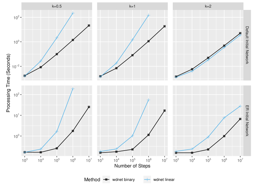
Figure 3: Algorithm runtime for weighted networks with default initial network (upper) of one edge $(1,2,1)$ and with initial weighted ER networks (lower) of $10^{4}$ nodes and $10^{6}$ edges. Edge weights, including those in the initial weighted ER networks, are drawn from Gamma(5, 0.2). Probability of edge schemes are $\alpha=\beta=\gamma=1/3$. Preference functions are $f_{1}(x,y)=x^{k}+0.1$, $f_{2}(x,y)=y^{k}+0.1$ with $k\in\left\{0.5,1,2\right\}$. Each point represents the median runtime of 100 replications.

The top three panels of Figure 3 compare the median runtimes of generating $100$ independent weighted, directed PA networks via binary and linear methods. When preference functions are sub-linear ($k=0.5$) or linear ($k=1$), the binary method is much more efficient than the linear method. Besides, the larger the number of steps is, the more advantageous it is to use the binary method. Some simulations for the linear method are omitted because they are excessively time-consuming. For a super-linear preference function ($k=2$), the difference in generation speed between the two methods becomes subtle. A further investigation reveals that the sum of source (and target) preference scores of the 20 earliest created nodes, $\{v_{1},v_{2},\ldots,v_{20}\}$, take $99\%$ of the total (for all nodes), making them dominant in the sampling process. Those early created nodes are always quickly selected under whichever edge addition scenario since linear search visits those “ancestors’ ’ first. Consequently, the time cost of using linear method is significantly reduced.

To further investigate the impact of early created nodes in the sampling process, we consider a modified (i.e., weighted and directed) Erdös–Rényi (ER) network (Erdös and Rényi, 1959; Gilbert, 1959) as an initial network. For each simulation run, we generate an ER network with $10^{4}$ nodes and $10^{6}$ edges, where edge weights are drawn independently from ${\rm Gamma}(5,0.2)$. We keep all other parameters same as in the previous experiment, and give the median runtime (of $100$ independently generated PA network replica) in the bottom three panels of Figure 3. We observe similar patterns for $k=0.5$ and $k=1$, so focus on $k=2$ only. Here the binary algorithm outperforms the linear method, since the large seed network alleviates the domination of old nodes in the subsequent sampling process.

In fact, most nodes that are sampled throughout the process are those with high strengths in the seed graph. Owing to the feature of ER network, a few hundred nodes (out of $10^{4}$) in the seed network are repeatedly sampled. However, a larger pool (compared to $20$ in the previous experiment) results in longer runtime when using the linear method. On the other hand, we believe the performance of linear algorithm will improve as $n$ gets larger since fewer nodes will continue to be dominant in the sampling process. Since we have added a sorting procedure in the linear algorithm, those nodes will be quickly selected. Accordingly, the linear method may finally outperform the binary method for extremely large networks. Last but not least, we find the tracing curves between $10^{3}$ and $10^{4}$ become flatter in the bottom plots when compared to their upper counterparts (for each $k$). This is due to the large seed graph, which requires a certain amount of time to initialize the sampling process. Consequently, there is a small difference in the total generation time for relatively small $n$.

Unweighted networks

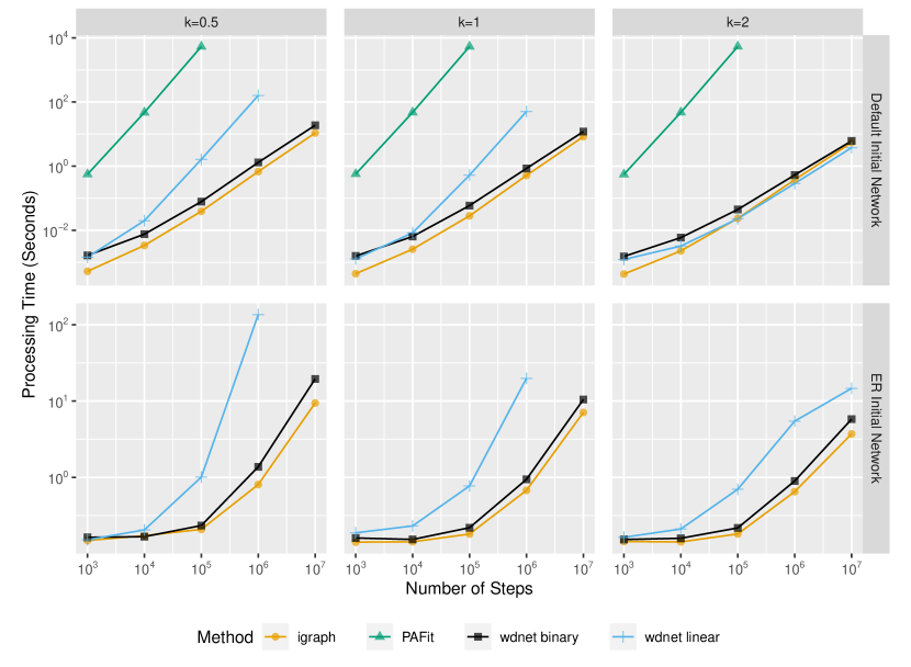
Figure 4: Algorithm runtime for unweighted networks with default initial network (upper) of one edge from $v_{1}$ to $v_{2}$ and with initial unweighted ER networks (lower) of $10^{4}$ nodes and $10^{6}$ edges. Probability of edge schemes are $\alpha=1$, $\beta=\gamma=0$. The target preference function is $f_{2}(x,y)=y^{k}+0.1$. Each point represents the median runtime of 100 replications.

Next, we compare the performance of generating unweighted PA networks using our package wdnet and the other two popular packages PAFit and igraph. Since PAFit and igraph allow the $\alpha$ scheme only, we now set $\alpha=1$ in the rpa_control_scenario() function. Under such setting, we only need to define a target preference function in the form of $f_{2}(x,y)=y^{k}+0.1$, where we again assume $k\in\left\{0.5,1,2\right\}$. Similar to the previous experiments, we generate unweighted PA networks with $n\in\left\{10^{3},\cdots,10^{7}\right\}$ for each $k$. A default initial network is adopted for each simulation run. The results are given in the top three panels of Figure 4. For $k=0.5$ and $k=1$, we find the binary algorithm in our package and igraph (psumtree method) are almost equally efficient, and outperform the rest. The performance of linear method in our package is better than PAFit (similar to linear search) since the former is implemented in C++ whereas the latter is implemented in R. For $k=2$, we do not see much difference among the two methods in our package wdnet and that in igraph, which is consistent with our conclusions for the weighted PA network generation experiment. Overall, PAFit is the least efficient, especially for generating large PA networks.

Lastly, we repeat our simulations by considering large ER networks as the initial graphs in order to alleviate the impact of few old nodes during the generation process. The setup is the same as that for weighted network simulations. Noticing that PAFit does not accept arbitrary initial networks, we exclude it from this set of simulation comparisons. The corresponding results are shown in the bottom three panels of Figure 4. Similar to the conclusions drawn for weighted PA networks, the binary method outperforms the linear method in our package owing to the less influence from old nodes when $k=2$. Moreover, there is little performance difference between the binary method and igraph across all considered $k$ values.

5 Discussions

Our R package wdnet provides useful tools to efficiently generate large-scale PA networks. The package admits a wide range of PA network specifications such as multiple edge addition scenarios, weighted and directed edges, and reciprocal edges. Our implementations extend those discussed in Wan et al. (2017) and Britton (2020), most of which are not available in other existing packages. A distinctive feature of the package is that it allow users to define their own preference functions. Our binary algorithm is efficient for general situations. Our linear algorithm outperforms implementations of the same algorithm in other packages due to its sorting step. The core implementation is in C++ for fast speed.

Efficient generation of PA networks facilitates investigation of PA networks properties and goodness-of-fit diagnosis in real applications. A PA network is controlled by many parameters. When theoretical properties, for example, transitivity and clustering coefficients, are challenging to derive, their empirical versions can be easily learned from generating many realizations given the model parameters. When the initial network size is large relative to the desired PA network size, its impact may not be ignorable and could be studied through simulations. In real applications, the goodness-of-fit diagnosis of a PA network can be done by generating many replicates from the fitted PA model and comparing the observed network statistics with the empirical distribution of the same statistics from the replicates. Such goodness-of-fit check may motivate modification of the PA networks to fit the real data better (e.g., Wang et al., 2022).

Beyond general PA network generation, wdnet also provides a collection of other functions. Specifically, several centrality measures are available via function centrality(), including the recently proposed weighted PageRank centrality (Zhang et al., 2022). Assortativity measures for weighted directed networks discussed in (Yuan et al., 2021) are available via function assortcoef(). A degree-preserving rewiring algorithm for generating networks with pre-determined assortativity coefficients (Wang et al., 2022) is available via function dprewire(). All these functions are derived from recent research, so they are not available in other packages.

Supplementary material

1. The code used for benchmarks and the R Markdown source for the paper can be found at https://github.com/Yelie-Yuan/code-sharing/tree/main/generating-pa.

2. The development version of the package is available at https://gitlab.com/wdnetwork/wdnet.

Funding

Dr. Wang and Dr. Yan’s works were partially supported by the NSF grant DMS2210735.

Appendix A Alternative sampling method for special cases

Fast sampling is available when source (target) preference functions are linear. We demonstrate this approach through an example of sampling source nodes with a preference function $f_{1}(x,y)=x+a_{5}$.

As shown in Section 2.1, the main idea of sampling is to make draws from a bag of node labels, where the number of labels is equal to the out-degrees. At step $t+1$, generate a random variable $U\sim{\rm Unif}(0,\sum_{v_{j}\in V(t)}\theta_{1}(v_{j},t))$, then the source node (for the new edge) is randomly drawn from the bag if $U\leq\sum_{v_{j}\in V(t)}\text{O}(v_{j},t)$. Otherwise, the source node is uniformly drawn from all existing nodes (regardless of their out-degrees). The sampling at each step has complexity $O(1)$, thus giving complexity $O(n)$ for the entire network generation process. The sampling of target nodes can be done in an analogous manner, and we call this approach bag in our package.

This idea can be generalized to weighted networks. At step $t+1$, the source preference score of node $v_{j}$ is

$$\sum_{k:(v_{j},v_{k},w_{jk})\in E(t)}w_{jk}+a_{5},$$

where total source preference of all existing nodes in the network is

$$\sum_{v_{j}\in V(t)}\left(\text{O}(v_{j},t)+a_{5}\right):=W(t)+a_{5}\,|V(t)|,$$

where $W(t)$ is the total weight and $|V(t)|$ is the cardinality of $V(t)$. The sampling process proceeds as follows:

1. At step $t+1$, create a vector, $\bm{\nu}(t)$, of cumulative sum of edge weights (according to the emergence order of edges), where the first element is $0$ and the last element is $W(t)$;

2. Compute $\tau(t+1)=(W(t)+a_{5}|V(t)|)X$ for some random variable $X\sim{\rm Unif}(0,1)$, independent from the network generation process;

3. If $\tau(t+1)>W(t)$, a node is randomly sampled from $V(t)$; otherwise, find an index $\ell$ such that $\tau(t+1)\in(\bm{\nu}_{\ell}(t),\bm{\nu}_{\ell+1}(t)]$, then select the source node of the edge corresponding to the $\ell$-th addition in $\bm{\nu}(t)$.

The sampling becomes efficient if we apply the above approach to all steps simultaneously. Notice that edge weights are independently drawn from $h$, and they are also independent of other network generation components. Hence, to efficiently generate networks after $n$ steps of evolution, vector $\bm{\nu}(n)$ can be determined independently in advance. Moreover, given a generated list of edge scenario parameters (i.e., $\alpha$, $\beta$ and $\gamma$), $|V(t)|$ can be obtained for $1\leq t\leq n$ as well. Therefore, we collect all information that we need for node sampling in the entire network generation process, i.e., $W(t)$ and $|V(t)|$ for $1\leq t\leq n$, with complexity $O(n)$. It remains to find the exact interval covering $\tau(t+1)$ in $\bm{\nu}(t)$ (a subset of $\bm{\nu}(n)$) for $\tau(t+1)\leq W(t)$, which can be done efficiently using the findInterval() function (with time complexity $O(n\log{n})$).

We wrap up the above sampling approach as bagx in our package. Although bagx is not as efficient as bag for generating unweighted, linear PA networks, it provides a competitive alternative to generating weighted PA networks compared with the standard algorithm.

Appendix B Advanced customized preference functions

Users can define customized preference functions by utilizing cppXPtr from package RcppXPrtUtils. The returned (external) pointer, XPtr, can be passed to spref and/or tpref. For instance, we fix the target preference function as $f_{2}(x,y)=y+1$, and set the source preference function to be

$$f_{1}(x,y)=\begin{cases}1&\qquad\text{if }x<1;\\ x^{2}&\qquad\text{if }1\leq x\leq 100;\\ 200(x-50)&\qquad\text{otherwise}.\end{cases}$$

The corresponding codes are given as follows:

my_spref <- RcppXPtrUtils::cppXPtr(code =

  "double foo(double x, double y) {

    if (x < 1) {

      return 1;

    } else if (x <= 100) {

      return pow(x, 2);

    } else {

      return 200 * (x - 50);

    }

  }")

ctr7 <- rpa_control_preference(ftype = "customized", spref = my_spref,

  tpref = "ins + 1")

External pointers cannot be shared across different R sessions. Therefore, we recommend that users save the source code of the customized preference functions for recompilation.

References

- Abbasi et al. (2012) Abbasi A, Hossain L, Leydesdorff L (2012). Betweenness centrality as a driver of preferential attachment in the evolution of research collaboration networks. Journal of Informatics, 6(3): 403–412.
- Atwood et al. (2015) Atwood J, Ribeiro B, Towsley D (2015). Efficient network generation under general preferential attachment. Computational Social Networks, 2(1): 7.
- Barabási and Albert (1999) Barabási AL, Albert R (1999). Emergence of scaling in random networks. Science, 286(5439): 509–512.
- Barrat et al. (2004) Barrat A, Barthélemy M, Vespignani A (2004). Weighted evolving networks: Coupling topology and weight dynamics. Physical Review Letters, 92(22): 228701.
- Bollobás et al. (2003) Bollobás B, Borgs C, Chayes J, Riordan O (2003). Directed scale-free graphs. In: SODA ’03: Proceedings of the Fourteenth Annual ACM-SIAM Symposium on Discrete Algorithms, 132–139. Society for Industrial and Applied Mathematics, Philadelphia, PA, USA.
- Britton (2020) Britton T (2020). Directed preferential attachment models: Limiting degree distributions and their tails. Journal of Applied Probability, 57(1): 122–136.
- Capocci et al. (2006) Capocci A, Servedio VDP, Colaiori F, Buriol LS, Donato D, Leonardi S, et al. (2006). Preferential attachment in the growth of social networks: The internet encyclopedia Wikipedia. Physical Review E, 74(3): 036116.
- Csardi and Nepusz (2006) Csardi G, Nepusz T (2006). The \pkgigraph software package for complex network research. InterJournal, Complex Systems: 1695.
- Dong et al. (2020) Dong X, Castro L, Shaikh N (2020). \pkgfastnet: An \proglangR package for fast simulation and analysis of large-scale social networks. Journal of Statistical Software, 96(7): 1–23.
- Eddelbuettel and François (2011) Eddelbuettel D, François R (2011). \pkgRcpp: Seamless \proglangR and \proglangC++ integration. Journal of Statistical Software, 40(8): 1–18.
- Erdös and Rényi (1959) Erdös P, Rényi A (1959). On random graphs I. Publicationes Mathematicae Debrecen, 6: 290–297.
- Gilbert (1959) Gilbert EN (1959). Random graphs. Annals of Mathematical Statistics, 30(4): 1141–1144.
- Hadian et al. (2016) Hadian A, Nobari S, Minaei-Bidgoli B, Qu Q (2016). ROLL: Fast in-memory generation of gigantic scale-free networks. In: SIGMOD ’16: Proceedings of the 2016 International Conference on Management of Data, 1829–1842. Association for Computing Machinery, New York, NY, USA.
- Hagberg et al. (2008) Hagberg AA, Schult DA, Swart PJ (2008). Exploring network structure, dynamics, and function using \pkgNetworkX. In: Proceedings of the 7th Python in Science Conferencee (SciPy 2008), 11–15. Pasadena, CA, USA.
- Kong et al. (2008) Kong JS, Sarshar N, Roychowdhury VP (2008). Experience versus talent shapes the structure of the web. Proceedings of the National Academy of Sciences, 105(37): 13724–13729.
- Mahmoud (1992) Mahmoud HM (1992). Evolution of Random Search Trees. John Wiley & Sons, Hoboken, NJ, USA.
- Mahmoud (2008) Mahmoud HM (2008). Pólya Urn Models. CRC Press, Boca Raton, FL, USA.
- Momeni and Rabbat (2015) Momeni N, Rabbat MG (2015). Measuring the generalized friendship paradox in networks with quality-dependent connectivity. In: Complex Networks VI: Proceedings of the 6th Workshop on Complex Networks CompleNet 2015 (G Mangioni, F Simini, SM Uzzo, D Wang, eds.), 45–55. Springer-Verlag.
- Pham et al. (2020) Pham T, Sheridan P, Shimodaira H (2020). \pkgPAFit: An \proglangR package for the non-parametric estimation of preferential attachment and node fitness in temporal complex networks. Journal of Statistical Software, 92(3): 1–30.
- Ucar (2022) Ucar I (2022). \pkgRcppXPtrUtils: XPtr Add-Ons for ‘\pkgRcpp’. \proglangR package version 0.1.2.
- Wan et al. (2017) Wan P, Wang T, Davis RA, Resnick SI (2017). Fitting the linear preferential attachment model. Electronic Journal of Statistics, 11(2): 3738–3780.
- Wang and Resnick (2022a) Wang T, Resnick SI (2022a). Asymptotic dependence of in-and out-degrees in a preferential attachment model with reciprocity. Extremes, 25(3): 417–450.
- Wang and Resnick (2022b) Wang T, Resnick SI (2022b). Random networks with heterogeneous reciprocity. ArXiv e-prints.
- Wang and Resnick (2023) Wang T, Resnick SI (2023). Poisson edge growth and preferential attachment networks. Methodology and Computing in Applied Probability, 25(1): 8.
- Wang et al. (2022) Wang T, Yan J, Yuan Y, Zhang P (2022). Generating directed networks with predetermined assortativity measures. Statistics and Computing, 32(5): 91.
- Yuan et al. (2023) Yuan Y, Wang T, Yan J, Zhang P (2023). \pkgwdnet: Weighted and Directed Networks. University of Connecticut. \proglangR package version 1.1.1.
- Yuan et al. (2021) Yuan Y, Yan J, Zhang P (2021). Assortativity measures for weighted and directed networks. Journal of Complex Networks, 9(2): cnab017.
- Zhang et al. (2022) Zhang P, Wang T, Yan J (2022). PageRank centrality and algorithms for weighted, directed networks. Physica A: Statistical Mechanics and its Applications, 586: 126438.