Time Series Forecasting via Semi-Asymmetric Convolutional Architecture with Global Atrous Sliding Window

Abstract

The proposed method in this paper is designed to address the problem of time series forecasting. Although some exquisitely designed models achieve excellent prediction performances, how to extract more useful information and make accurate predictions is still an open issue. Most of modern models only focus on a short range of information, which are fatal for problems such as time series forecasting which needs to capture long-term information characteristics. As a result, the main concern of this work is to further mine relationship between local and global information contained in time series to produce more precise predictions. In this paper, to satisfactorily realize the purpose, we make three main contributions that are experimentally verified to have performance advantages. Firstly, original time series is transformed into difference sequence which serves as input to the proposed model. And secondly, we introduce the global atrous sliding window into the forecasting model which references the concept of fuzzy time series to associate relevant global information with temporal data within a time period and utilizes central-bidirectional atrous algorithm to capture underlying-related features to ensure validity and consistency of captured data. Thirdly, a variation of widely-used asymmetric convolution which is called semi-asymmetric convolution is devised to more flexibly extract relationships in adjacent elements and corresponding associated global features with adjustable ranges of convolution on vertical and horizontal directions. The proposed model in this paper achieves state-of-the-art on most of time series datasets provided compared with competitive modern models.

1 Introduction

Time series is a sequence taken at successive equally spaced points in time which is also known as dynamic series. Precise prediction of time series has close connections to human society, for instance, it may help people format schedules and company make adjustments on investment strategy. Moreover, foreseeing future behaviour based on analysis of known historical data is of great importance in lots of fields such as epidemic [1], medical treatment [2], finance [3, 4] and industrial Internet [5]. Time series forecasting therefore attracts attention from researchers around the world. Nevertheless, how to fully utilize observation to generate accurate and reasonable predictions is still an unsolved problem.

To realize accurate prediction of future, researchers develop various kinds of solutions. RNN model has been favored by researchers since it was proposed. Because of its recurrent architecture design, RNN models can effectively model long-term dependencies [11], therefore achieve an effective understanding of temporal data [12, 13] as well. However, RNN may encounter memory overflow due to continuous storage of previous states and gradient vanishing problems. To further make up for shortcomings of RNN, an improved solution based on it is proposed which is called LSTM [14]. Its core concepts are the memory cell states that allow information to be passed on backwards, and the gate structures that allow certain information to be added and removed. Coincidentally, researchers also find that temporal task can also benefit form LSTM’s characteristics [15, 16]. In a quite long period of time, the model based on RNN has played an important role in development of time series forecasting. Recently, transformer-based models [6, 7, 8, 9] have been proposed enormously, which applied self-attention mechanism to distill useful semantic information in time series. However, there exists a doubt that transformer-like structure is not suitable for the task of time series forecasting. Under certain circumstances, the performance of the models can not even match ingeniously designed linear model [10], which has shaken the position of transformer-based models in time series forecasting. At present, the controversy still continues. Besides, there also exist lots of meaningful works trying to satisfy demand of time series forecasting from other multiple aspects as well [17].

Moreover, CNN-based models are also widely utilized for prediction of temporal data. They are mainly divided into two categories, one is the variation of causal and dilated convolution [18], the other is algorithms using graph convolutional neural network [19] to solve corresponding problems. Generally, it can be concluded that transformer and CNN models, the two well-established solutions in the field of computer vision, also achieve excellent performance in tasks of time series forecasting. Back to CNN-based models, there have been many new CNN models in recent years, for instance, temporal convolutional network (TCN) [20], convolutionally low-rank model [21] and non-pooling CNN [22]. Among them, TCN attracts the most attention which is capable of large-scale parallel processing and managing a series of sequences of arbitrary length and uniformly output sequences with the same length. Specifically, the casual and dilated convolution introduced by it enable CNN forecasting model to possess a larger receptive field to better acquire information in a longer range under strict time restrictions. Moreover, other effective models [23, 24, 25] also improve performance by enlarging ranges of data selection and more ingenious and flexible extraction of relationships of adjacent and non-adjacent elements because of similar considerations about demand of time series forecasting mentioned above. Nevertheless, it is noting that all of the models still receive data in a relatively restricted way without considering global data features.

To address the issue, we design a kind of data reconstruction method referencing solution based on partitioned universe of discourse [26] partly which transforms original temporal data into difference sequence [27, 28, 29] ensuring that the model is more likely dealing with steady-state sequences and associates relative positional information of data captured in the view of whole observation time series to reduce difficulty of model learning to some extent. More than that, we choose to replace all of elements by the last one only keeping their positional information as subsidiaries to maximize timeliness of data without losing too much semantic information of temporal data. Besides, the relationship among converted information in different subsections and time series are probably separate [30], so there is a need to devise a convolution strategy with different directions and shapes to further mine underlying information. Due to particularity of time series, traditional squared convolution is not capable to manage complex extraction of relationship of elements in temporal data, a variation of asymmetric convolution [31, 32] which is called semi-asymmetric convolution is designed accordingly. The semi-asymmetric convolution is divided into horizontal and vertical filters, and they probably possess different length to retrieve interaction information at a more fine-grained level in selected fragments from difference series. The advantage of this improvement is that it is able to effectively obtain temporal features using adjustable scales [33, 34], and speeding up the training and inference process of the proposed model [35] at the same time. In general, the major contributions of this work are summarized as follows:

1. The input to proposed model is difference sequences transformed by original observation time series to enable model to learn more easily

2. A new kind of method of data reconstruction is designed to endow each elements with their corresponding relative positional information

3. A novel convolutional architecture called semi-asymmetric convolution with flexible scales is designed to acquire information at different levels.

The rest of this paper is organized as follows. In the second section, some related concepts of the proposed model are introduced. And the details of the proposed model are presented in the third section. Besides, the fifth section provides experimental results and corresponding discussions with respect to models. In the last section, conclusions and outlook of future work are given.

2 Preliminary

In this section, related concepts about the proposed model are briefly introduced.

2.1 Difference of First Order

A first order difference is the difference between two consecutive adjacent terms in a discrete function. Assume there exists a function $y=f(x)$, $y$ is defined only on the non-negative integer value of $x$ and when the independent variable $x$ is iterated through the non-negative integers in turn, namely $x=0,1,2,...$, the corresponding values of function can be defined as:

$$f(0),f(1),f(2),...$$ (1)

it can be abbreviated as:

$$y_{0},y_{1},y_{2},...$$ (2)

when the independent value changes from $x$ to $x+1$, the variation of $y=f(x)$ can be defined as:

$$\Delta y_{x}=f(x+1)-f(x),(x=1,2,3,...)$$ (3)

it’s called the first difference of the function $y(x)$ at point $x$ which is usually denoted as:

$$\Delta y_{x}=y_{x+1}-y_{x},(x=1,2,3,...)$$ (4)

2.2 Asymmetric Convolution Architecture

CNN has embraced a quick development recently, it is widely applied in different fields, such as time series and computer vision [36, 37, 38] due to its stable and excellent performance. For an operation of convolving, assume an input $\varsigma\in\mathbb{R}^{H\times W}$ and filter $\mathbb{C}$, the process of generating output $\lambda\in\mathbb{R}^{H^{\prime}\times W^{\prime}}$ can be defined as:

$$\lambda=\mathbb{C}*\varsigma,\quad\varsigma\in\mathbb{R}^{H\times W},\lambda\in\mathbb{R}^{H^{\prime}\times W^{\prime}},\mathbb{C}\in\mathbb{R}^{d\times d}$$ (5)

where $*$ is the 2D convolution operator. Moreover, asymmetric convolution [39, 35] is considered as an economical choice to approximate an existing square-kernel convolutional layer for obtaining acceleration and compression. Specifically, the original filter can be decomposed into horizontal and vertical filters, $\mathbb{C}_{h},\mathbb{C}_{v}$, respectively, which can be defined as:

$$\mathbb{C}*\varsigma=\mathbb{C}_{v}*(\mathbb{C}_{h}*\varsigma),\mathbb{C}_{v}\in\mathbb{R}^{d\times 1},\mathbb{C}_{h}\in\mathbb{R}^{1\times d}$$ (6)

compared with the original convolution utilizing $d\times d$ kernel size, the time complexity changes from $\mathcal{O}((d^{2}H^{\prime}W^{\prime})$ to $\mathcal{O}(2dH^{\prime}W^{\prime})$. Due to efficiency of the asymmetric architecture, it is widely applied in convolutional neural network design [40, 41] and gains performance improvement generally.

2.3 Atrous Algorithm

The atrous algorithm is proposed in [42, 43] which is also known as dilated convolution. Assume there exists a one-dimensional input $\alpha[s]$, the corresponding output $\beta[s]$ of dilated convolution via a filter $\omega[e]$ with length $E$ can be defined as:

$$\beta[s]=\sum_{e=1}^{E}\alpha[s+r\cdot e]\omega[e]$$ (7)

where rate parameter $r$ is corresponding to the stride and standard convolution is a special case for $r=1$. Generally, atrous algorithm is designed to avoid precision loss brought by reduction of feature map on account of multiple convolutional and pooling layers on vision tasks and is broadly utilized in many other import fields, such as audio processing [44] and time series forecasting [20].

2.4 Naive Forecasting

The naive forecasting is the simplest prediction method in the field of time series which regards the most recent observation value as the prediction of future. Assume there exists a time series $\mathbb{T}$ with a length $n$ which can be defined as:

$$\mathbb{T}=\{(t_{1},\zeta_{1}),(t_{2},\zeta_{2}),...,(t_{n-1},\zeta_{n-1}),(t_{n},\zeta_{n})\}$$ (8)

where $\zeta_{i},i\in[1,n]$ represents observation value at time point $i$. For example, if there is a need to predict $\zeta_{n+q}$ which is unknown, the value of $\zeta_{n}$ can be referenced as the prediction value of $\zeta_{n+q}$ directly. Assume the prediction value of $\zeta_{n+q}$ is $\hat{\zeta}_{n+q}$, then the method of forecasting can be defined as:

$$\hat{\zeta}_{n+q}=\zeta_{n}$$ (9)

under various circumstances, naive forecasting is an effective solution to tell the future trend of time series like stock price prediction. Nevertheless, the method introduced is not a satisfying solution in time series forecasting, but it can provide a benchmark for other prediction methods.

2.5 Fuzzy Time Series

One of concepts of fuzzy time series is introduced by Chen [26] which is developed based on theories proposed in [45, 46, 47]. The method of fuzzy time series could extract information effectively by utilizing overall characteristics of time series data and provide stable performance. Specifically, given a time series $\mathbb{T}$, and let $\eta_{min}$ and $\eta_{max}$ be minimum and maximum value in $\mathbb{T}$, the four steps to generate fuzzy time series can be presented as:

Step 1: Select two proper positive numbers $\eta_{1}$ and $\eta_{2}$, a universe of discourse $\mathbb{U}$ can be defined as $[\eta_{min}-\eta_{1},\eta_{max}-\eta_{2}]$

Step 2: Partition $\mathbb{U}$ into segments with equal length $\{u_{1},u_{2},...u_{m}\}$ which is called fuzzy intervals

Step 3: Let $\mathbb{Z}_{1},\mathbb{Z}_{2},...,\mathbb{Z}_{k}$ be fuzzy sets and they are defined on universe of discourse $\mathbb{U}$ as:

$$\left\{\begin{array}[]{l}\mathbb{Z}_{1}=z_{11}/u_{1}+z_{12}/u_{2}+...+z_{1m}/u_{m},\\ \mathbb{Z}_{2}=z_{21}/u_{1}+z_{22}/u_{2}+...+z_{2m}/u_{m},\\ \vdots\\ \mathbb{Z}_{k}=z_{k1}/u_{1}+z_{k2}/u_{2}+...+z_{km}/u_{m}\end{array}\right.$$ (10)

where $z_{ij}\in[0,1],i\in[1,k],j\in[1,m]$ and the value of $z_{ij}$ represents the degree of membership of $u_{j}$ in fuzzy set $\mathbb{Z}_{i}$.

Step 4: The derived fuzzy logical relationships which possess identical initial states are divided into the same group. Then, the matches between actual values in time series and groups of fuzzy logical relationships can be acquired.

After these four steps, the original data is transformed into fuzzy time series.

3 Architecture of the Proposed Forecasting Model

In this section, the proposed forecasting model based on relevant concepts mentioned above is introduced.

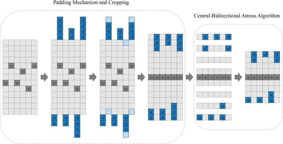
Figure 1: Padding Mechanism, Cropping and Central-Bidirectional Atrous Algorithm with Dilation Factor $d=1$

3.1 Difference Layer: Convert Time Series into First Order Difference Sequence

First, a time series $\mathbb{T}$ is transformed into its first order difference sequence $\mathbb{T}_{\Delta}$. The process can be given as:

$$\left\{\begin{array}[]{l}\mathbb{T}=\{(t_{1},\zeta_{1}),(t_{2},\zeta_{2}),...,(t_{n-1},\zeta_{n-1}),(t_{n},\zeta_{n})\}\\ \qquad\qquad\qquad\qquad\qquad\Downarrow\\ \mathbb{T}_{\Delta}^{-}=\{(t_{2,1},\zeta_{2}-\zeta_{1}),...,(t_{n,n-1},\zeta_{n}-\zeta_{n-1})\}\\ \qquad\qquad\quad\Downarrow\\ \mathbb{T}_{\Delta}=\{\alpha_{1},\alpha_{2},...,\alpha_{h}\}\\ \end{array}\right.$$ (11)

where $h=n-1$ and $\alpha_{i},i\in[1,h]$ only contains observed value without timestamp. Obviously, it can be obtained that the length of $\mathbb{T}_{\Delta}$ is $n-1$. In the next step, the input is $\mathbb{T}_{\Delta}$ instead of $\mathbb{T}$.

3.2 Division layer: Divide Converted Time Series into Sub-Series Based on Sliding Window

Second, series $\mathbb{T}_{\Delta}$ is divided by sliding window whose size is $\mathbb{W}$ into sub-series, the segmented data fragments are:

$$\mathbb{T}_{\Delta}^{Seg}=\{\varUpsilon_{1},\varUpsilon_{2},...,\varUpsilon_{c}\},c=h-\mathbb{W}+1$$ (12)

where $\varUpsilon_{j}=\{\alpha_{j},\alpha_{j+1},...,\alpha_{j+\mathbb{W}-1}\},j\in[1,c]$.

3.3 Encoder of segmented sequences

3.3.1 Relative Positional Encoding: Reconstruct Sub-Series with View on Global Observation Temporal Data

Third, in the concept of fuzzy time series proposed in [26], the two numbers $\eta_{1}$ and $\eta_{2}$ are selected intuitively, which may lead to non-reproducibility of experiment results on various datasets. As a result, $\eta_{1}$ and $\eta_{2}$ are uniformly set as standard deviation of corresponding first order difference sequence, which can be given as:

$$\varphi=\eta_{1}=\eta_{2}=\sigma(\mathbb{T}_{\Delta})$$ (13)

where $\sigma$ represents standard deviation. Then, universe of discourse $\mathbb{U}$ of $\mathbb{T}_{\Delta}$ can be calculated as:

$$\mathbb{U}_{\mathbb{T}_{\Delta}}=[\alpha_{min}-\varphi,\alpha_{max}+\varphi]=[\beta_{l},\beta_{u}]$$ (14)

where $\alpha_{min}$ and $\alpha_{max}$ represent minimum and maximum element contained in $\mathbb{T}_{\Delta}$ and $\beta_{l}$ and $\beta_{u}$ denote lower and upper bound of $\mathbb{U}_{\mathbb{T}_{\Delta}}$. And the number of intervals, $\mathbb{N}$, can be confirmed as:

$$\mathbb{N}=log_{2}^{h}-1$$ (15)

the partitioned universe of discourse can be given as:

$$\mathbb{U}_{\mathbb{T}_{\Delta}}=[\beta_{l},\beta_{l}+\xi,...,\beta_{l}+\kappa\times\xi,...,\beta_{u}-\xi,\beta_{u}]$$ (16)

where $\xi=(\beta_{u}-\beta_{l})/\mathbb{N}$ and $\kappa\in[1,\mathbb{N}]$. Then, integrate each element contained in $\varUpsilon_{j}$ into the partitioned universe of discourse $\mathbb{U}_{\mathbb{T}_{\Delta}}$ to create new sequences based on data fragments captured by sliding window:

$$\tiny\varUpsilon_{j}^{\mathbb{U}_{\mathbb{T}_{\Delta}}}=\begin{bmatrix}\beta_{l}&...&\beta_{l}+\kappa^{\prime}\times\xi&\alpha_{j}&\beta_{l}+(\kappa^{\prime}+1)\times\xi&...&\beta_{u}\\ \beta_{l}&...&\beta_{l}+\kappa^{\prime\prime}\times\xi&\alpha_{j+1}&\beta_{l}-(\kappa^{\prime\prime}+1)\times\xi&...&\beta_{u}\\ \vdots&\vdots&\vdots&\vdots&\vdots&\vdots&\vdots\\ \beta_{l}&...&\beta_{l}+\kappa^{\prime\prime\prime}\times\xi&\alpha_{j+\mathbb{W}-1}&\beta_{l}-(\kappa^{\prime\prime\prime}+1)\times\xi&...&\beta_{u}\end{bmatrix}$$ (17)

the position of each integrated element is uniquely identified. Then, all the data from sliding window in the reconstructed series is replaced with the last element in original subset divided only keeping position information of former elements:

$$\scriptsize\ell_{j}=\begin{bmatrix}\beta_{l}&...&\beta_{l}+\kappa^{\prime}\times\xi&\alpha_{j+\mathbb{W}-1}&\beta_{l}+(\kappa^{\prime}+1)\times\xi&...&\beta_{u}\\ \beta_{l}&...&\beta_{l}+\kappa^{\prime\prime}\times\xi&\alpha_{j+\mathbb{W}-1}&\beta_{l}+(\kappa^{\prime\prime}+1)\times\xi&...&\beta_{u}\\ \vdots&\vdots&\vdots&\vdots&\vdots&\vdots&\vdots\\ \beta_{l}&...&\beta_{l}+\kappa^{\prime\prime\prime}\times\xi&\alpha_{j+\mathbb{W}-1}&\beta_{l}+(\kappa^{\prime\prime\prime}+1)\times\xi&...&\beta_{u}\end{bmatrix}$$ (18)

the simplified form of it can be given as:

$$\ell_{j}=\begin{bmatrix}\beta_{l}&...&x_{1}&\underline{\alpha}&\mathring{x}_{1}&...&\beta_{u}\\ \beta_{l}&...&x_{2}&\underline{\alpha}&\mathring{x}_{2}&...&\beta_{u}\\ \vdots&\vdots&\vdots&\vdots&\vdots&\vdots&\vdots\\ \beta_{l}&...&x_{p}&\underline{\alpha}&\mathring{x}_{p}&...&\beta_{u}\\ \end{bmatrix}$$ (19)

where $p\in[1,\mathbb{W}]$ and the final input to the proposed network is:

$$\mathbb{T}_{Input}=\{\ell_{1},\ell_{2},...,\ell_{c}\}$$ (20)

3.3.2 Padding Mechanism and Cropping

Forth, one side of each row of input data is filled separately so that the length of data on both sides of the last element in original subset is the same. Assume data of row $p$ in $\ell_{\hbar}$ is vector $\vec{\varLambda_{p}}$, the process of padding can be given as:

$$\small\vec{\breve{\varLambda}}_{p}=\left\{\begin{array}[]{l}Concat(rep(\beta_{l})_{\mathbb{D}},\vec{\varLambda}_{p}^{\beta_{l}\Rightarrow x_{p}}),||(\vec{\varLambda}_{p}^{\beta_{l}\Rightarrow x_{p}})||<||(\vec{\varLambda}_{p}^{\mathring{x}_{p}\Rightarrow\beta_{u}})||\\ Concat(\vec{\varLambda}_{p}^{\mathring{x}_{p}\Rightarrow\beta_{u}},rep(\beta_{u})_{\mathbb{D}^{\prime}}),||(\vec{\varLambda}_{p}^{\beta_{l}\Rightarrow x_{p}})||>||(\vec{\varLambda}_{p}^{\mathring{x}_{p}\Rightarrow\beta_{u}})||\\ \end{array}\right.$$ (21)

where $\vec{\varLambda}_{p}^{\dot{o}\Rightarrow\ddot{o}}$ represents a segmented vector which ranges from element $\dot{o}$ to $\ddot{o}$, $||\vec{\varLambda}_{p}^{\dot{o}\Rightarrow\ddot{o}}||$ is the length of $\vec{\varLambda}_{p}^{\dot{o}\Rightarrow\ddot{o}}$ and $Concat$ denotes the operation of concatenation of two vectors. Besides, $rep(\dot{o})_{\mathbb{D}}$ means creating a vector containing $\mathbb{D}$ copies of element $\dot{o}$ and $\mathbb{D}=||(\vec{\varLambda}_{p}^{\mathring{x}\Rightarrow\beta_{u}})||-||(\vec{\varLambda}_{p}^{\beta_{l}\Rightarrow x})||$ or $\mathbb{D}^{\prime}=||(\vec{\varLambda}_{p}^{\beta_{l}\Rightarrow x})||-||(\vec{\varLambda}_{p}^{\mathring{x}\Rightarrow\beta_{u}})||$.

Then, each row containing in $\ell_{\hbar}$ is padded ensuring lengths of two sides of the last element in original subset are equal. However, the operation of padding brings a problem that length of each row is not exactly the same which is difficult for neural network to acquire information and capture features. As a result, there is a need to crop redundant elements in each padded data row. Assume length of the shortest padded vector is $\mathbb{S}$ and the operation of cropping $\mathbb{M}$ elements which lie from both ends of the vector $\breve{\varLambda}_{p}$ to its centre is $Crop_{\mathbb{M}}$, the process of cropping is defined as:

$$\underline{\vec{\varLambda}}_{p}=Crop_{\mathbb{M}}(\vec{\breve{\varLambda}}_{p})$$ (22)

where $\mathbb{M}=(||\vec{\breve{\varLambda}}_{p}||-\mathbb{S})/2$ and $\underline{\vec{\varLambda}}_{p}$ is the cropped vector.

3.3.3 Central-Bidirectional Atrous Algorithm

Fifth, the processed information needs to be further extracted so that subsequent networks can capture more useful information and avoid unnecessary calculations. Because of the unique nature of the reconstructed timing data, the atrous algorithm is modified to obtain data from the centre to both sides of each segment, which reserves the nearest observation value and corresponding position distribution information from the prediction object. Assume the leftmost and rightmost element in $\underline{\vec{\varLambda}}_{p}$ are $\epsilon_{l_{p}}$ and $\epsilon_{r_{p}}$, the input which is divided into two parts by the central element to central-bidirectional atrous algorithm (CBAA) is:

$$\left\{\begin{array}[]{l}\ell_{j}^{l}=[\underline{\vec{\varLambda}}_{1_{\mathring{x}_{1}+g\times d}}^{\ \mathring{x}_{1}\Rightarrow\epsilon_{r_{1}}},\underline{\vec{\varLambda}}_{2_{\mathring{x}_{2}+g\times d}}^{\ \mathring{x}_{2}\Rightarrow\epsilon_{r_{2}}},...,\underline{\vec{\varLambda}}_{{p-1}_{\mathring{x}_{p-1}+g\times d}}^{\ \mathring{x}_{p-1}\Rightarrow\epsilon_{r_{p-1}}},\underline{\vec{\varLambda}}_{p_{\mathring{x}_{p}+g\times d}}^{\ \mathring{x}_{p}\Rightarrow\epsilon_{r_{p}}}]\\ \ell_{j}^{r}=[{\mathchoice{\vbox{\offinterlineskip\halign{#\cr\reflectbox{$\displaystyle\vec{}\mkern 4.0mu$}\cr\kern-4.30554pt\cr$\displaystyle\underline{\varLambda}$\cr}}}{\vbox{\offinterlineskip\halign{#\cr\reflectbox{$\textstyle\vec{}\mkern 4.0mu$}\cr\kern-4.30554pt\cr$\textstyle\underline{\varLambda}$\cr}}}{\vbox{\offinterlineskip\halign{#\cr\reflectbox{$\scriptstyle\vec{}\mkern 4.0mu$}\cr\kern-3.01389pt\cr$\scriptstyle\underline{\varLambda}$\cr}}}{\vbox{\offinterlineskip\halign{#\cr\reflectbox{$\scriptscriptstyle\vec{}\mkern 4.0mu$}\cr\kern-2.15277pt\cr$\scriptscriptstyle\underline{\varLambda}$\cr}}}}_{1_{x_{1}-g\times d}}^{\epsilon_{l_{1}}\Rightarrow x_{1}},{\mathchoice{\vbox{\offinterlineskip\halign{#\cr\reflectbox{$\displaystyle\vec{}\mkern 4.0mu$}\cr\kern-4.30554pt\cr$\displaystyle\underline{\varLambda}$\cr}}}{\vbox{\offinterlineskip\halign{#\cr\reflectbox{$\textstyle\vec{}\mkern 4.0mu$}\cr\kern-4.30554pt\cr$\textstyle\underline{\varLambda}$\cr}}}{\vbox{\offinterlineskip\halign{#\cr\reflectbox{$\scriptstyle\vec{}\mkern 4.0mu$}\cr\kern-3.01389pt\cr$\scriptstyle\underline{\varLambda}$\cr}}}{\vbox{\offinterlineskip\halign{#\cr\reflectbox{$\scriptscriptstyle\vec{}\mkern 4.0mu$}\cr\kern-2.15277pt\cr$\scriptscriptstyle\underline{\varLambda}$\cr}}}}_{2_{x_{2}-g\times d}}^{\epsilon_{l_{2}}\Rightarrow x_{2}},...,{\mathchoice{\vbox{\offinterlineskip\halign{#\cr\reflectbox{$\displaystyle\vec{}\mkern 4.0mu$}\cr\kern-4.30554pt\cr$\displaystyle\underline{\varLambda}$\cr}}}{\vbox{\offinterlineskip\halign{#\cr\reflectbox{$\textstyle\vec{}\mkern 4.0mu$}\cr\kern-4.30554pt\cr$\textstyle\underline{\varLambda}$\cr}}}{\vbox{\offinterlineskip\halign{#\cr\reflectbox{$\scriptstyle\vec{}\mkern 4.0mu$}\cr\kern-3.01389pt\cr$\scriptstyle\underline{\varLambda}$\cr}}}{\vbox{\offinterlineskip\halign{#\cr\reflectbox{$\scriptscriptstyle\vec{}\mkern 4.0mu$}\cr\kern-2.15277pt\cr$\scriptscriptstyle\underline{\varLambda}$\cr}}}}_{{p-1}_{x_{p-1}-g\times d}}^{\epsilon_{l_{p-1}}\Rightarrow x_{p-1}},{\mathchoice{\vbox{\offinterlineskip\halign{#\cr\reflectbox{$\displaystyle\vec{}\mkern 4.0mu$}\cr\kern-4.30554pt\cr$\displaystyle\underline{\varLambda}$\cr}}}{\vbox{\offinterlineskip\halign{#\cr\reflectbox{$\textstyle\vec{}\mkern 4.0mu$}\cr\kern-4.30554pt\cr$\textstyle\underline{\varLambda}$\cr}}}{\vbox{\offinterlineskip\halign{#\cr\reflectbox{$\scriptstyle\vec{}\mkern 4.0mu$}\cr\kern-3.01389pt\cr$\scriptstyle\underline{\varLambda}$\cr}}}{\vbox{\offinterlineskip\halign{#\cr\reflectbox{$\scriptscriptstyle\vec{}\mkern 4.0mu$}\cr\kern-2.15277pt\cr$\scriptscriptstyle\underline{\varLambda}$\cr}}}}_{p_{x_{p}-g\times d}}^{\epsilon_{l_{p}}\Rightarrow x_{p}}]\\ \end{array}\right.$$ (23)

where $\ell_{j}^{l}$ and $\ell_{j}^{r}$ denote left and right part of cropped vector $\underline{\vec{\varLambda}}_{p}$ and the directions of filters on them are opposite. Moreover, assume a filter $f:\{0,...,v-1\}$ and the operation of CBAA, $\mathbb{F}$, starting with elements $\mathring{x}_{p}$ and $x_{p}$ is defined as:

$$\footnotesize\mathbb{F}(\underline{\alpha})_{j}=Concat(\sum_{g=0}^{v-1}f(g)\cdot\ell_{j}^{l},\underline{\alpha},\sum_{g=0}^{v-1}f(g)\cdot\ell_{j}^{r})$$ (24)

where $\cdot$ represents the operation of dilated convolution, $d$ is the factor of dilation, $v$ means the filter size, $\mathring{x}_{p}+g\times d$ and $x_{p}-g\times d$ account for the direction of movement of filters.

When $d=1$, the form of atrous algorithm degenerates into regular convolution. A larger dilation factor enables the algorithm to capture features at a longer range. In original atrous algorithm, the operation of dilation is utilized to enlarge the receptive field without reduce sizes of feature maps. But in the CBAA, the dilated convolution is mainly used to construct efficient maps with proper sizes containing underlying features of historic information via multiple non-adjacent fuzzy intervals.

3.4 Semi-Asymmetric Convolutional Architecture

Sixth, a semi-asymmetric convolutional neural network (SACNN) is designed to aggregate information and produce differential predictions. SACNN is made up of a stack of one module which is called SAC block. The SAC block consists of two parts, the first part is the batchnorm layer $Bn$ which is defined as:

$$\tilde{C}_{j}=Bn(\mathbb{F}(\underline{\alpha})_{j})=\frac{\mathbb{F}(\underline{\alpha})_{j}-\bar{\mathbb{F}(\underline{\alpha})_{j}}}{\sqrt{\sigma(\mathbb{F}(\underline{\alpha})_{j})+\epsilon}}*\gamma+\delta$$ (25)

where $\bar{\mathbb{F}(\underline{\alpha})_{j}}$ and $\sigma(\mathbb{F}(\underline{\alpha})_{j})$ denotes mean and standard-deviation of $\mathbb{F}(\underline{\alpha})_{j}$, $\gamma$ and $\delta$ are learnable parameter vectors whose size is the number of channel of input. The output $\tilde{A}_{j}$ is supposed to be sent into the next part, semi-asymmetric convolutional layer $Sa$ which consists of $L$ combinations of $X$ horizontal and vertical filters $\check{f}_{V}\in\mathbb{R}^{V\times 1}$ and $\check{f}_{H}\in\mathbb{R}^{1\times H}$ . Assume the input $\tilde{C}_{j}\in\mathbb{R}^{H^{\prime}\times V^{\prime}\times Y}$ with $H^{\prime}\times V^{\prime}$ feature map and $Y$ channels, the process of generating output can be defined as:

$$B_{j}=Sa(\tilde{C}_{j})=[\check{f}_{V}\diamond(\check{f}_{H}\diamond\tilde{C}_{j})]_{\times L},\ B_{j}\in\mathbb{R}^{H^{\prime\prime}\times V^{\prime\prime}\times X}$$ (26)

where $\diamond$ represents semi-asymmetric convolution and $OUT=X/Y$ is the lifting factor of number of input’s to output’s channels. When $V=H$, $Sa$ degenerates into the form of regular asymmetric convolution. Before outputting the final values, the information is expected to be sent into two linear layers:

$$Q_{j}=SAC(\mathbb{F}(\underline{\alpha})_{j})=(B_{j}A^{T}+b)A^{\prime T}+b^{\prime}$$ (27)

where $A$ and $A^{\prime}$ are the learnable weights of the module of shape which is transposed to times the original input $B_{j}$ and $b$ and $b^{\prime}$ are the biases to be added. Then, $Q_{j}$ is the prediction which the proposed model produce on the first order difference sequence $\mathbb{T}_{\Delta}$.

3.5 Restore Output of Network to Original Position and Make Prediction

Seventh, restore the differential prediction $Q_{j}$ to the original time series $\mathbb{T}$. The process of a sliding window generating corresponding prediction is given as:

$$\hat{\zeta}_{j+\mathbb{W}+1}=\zeta_{j+\mathbb{W}}+Q_{j}$$ (28)

on the training data, the proposed model is expected to approximate trend of changes of time series. For the prediction of value beyond the known time series data, the prediction is made as:

$$\hat{\zeta}_{n+1}=\zeta_{n}+Q_{n-\mathbb{W}}$$ (29)

the process of producing prediction of the proposed model is illustrated in Fig.2.

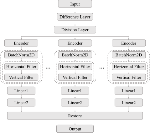
Figure 2: Details of the Proposed Model

TABLE I: MEAN MAE RESULTS OF UNIVARIATE DATASETS

Dataset	Naive	SES	Theta	TBATS	ETS	ARIMA	PR	CatBoost	FFNN	DeepAR
M1 Yearly	221512.32	171353.41	152799.26	103006.90	146110.11	145608.87	134246.38	215904.20	136238.80	152084.40
M1 Quarterly	3350.81	2206.27	1981.96	2326.46	2088.15	2191.10	1630.38	1802.18	1617.39	1951.14
M1 Monthly	2866.26	2259.04	2166.18	2237.50	1905.28	2080.13	2088.25	2052.32	2162.58	1860.81
M3 Yearly	1563.64	1022.27	957.40	1192.85	1031.40	1416.31	1018.48	1163.36	1082.03	994.72
M3 Quarterly	711.65	571.96	486.31	561.77	513.06	559.40	519.30	593.29	528.47	519.35
M3 Monthly	1002.94	743.41	623.71	630.59	626.46	654.80	692.97	732.00	692.48	728.81
M3 Other	452.11	277.83	215.35	189.42	194.98	193.02	234.43	318.13	240.17	247.56
M4 Yearly	1487.58	1009.06	890.51	960.45	920.66	1067.16	875.76	929.06	-	-
M4 Quarterly	838.19	622.57	574.34	570.26	573.19	604.51	610.51	609.55	631.01	597.16
M4 Monthly	835.69	625.24	563.58	589.52	582.60	575.36	596.19	611.69	612.52	615.22
M4 Weekly	480.94	336.82	333.32	296.15	335.66	321.61	293.21	364.65	338.37	351.78
M4 Daily	255.42	178.27	178.86	176.60	193.26	179.67	181.92	231.36	177.91	299.79
M4 Hourly	399.84	1218.06	1220.97	386.27	3358.10	1310.85	257.39	285.35	385.49	886.02
Tourism Yearly	117966.55	95579.23	90653.60	94121.08	94818.89	95033.24	82682.97	79567.22	79593.22	71471.29
Tourism Quarterly	13988.39	15014.19	7656.49	9972.42	8925.52	10475.47	9092.58	10267.97	8981.04	9511.37
Tourism Monthly	3019.44	5302.10	2069.96	2940.08	2004.51	2536.77	2187.28	2537.04	2022.21	1871.69
CIF 2016	650535.53	581875.97	714818.58	855578.40	642421.42	469059.49	563205.57	603551.30	1495923.44	3200418.00
Aus. Electricity Demand	241.77	659.60	665.04	370.74	1282.99	1045.92	247.18	241.77	258.76	302.41
Dominick	5.86	5.70	5.86	7.08	5.81	7.10	8.19	8.09	5.85	5.23
Bitcoin	6.57$\times$1017	5.33$\times$1018	5.33$\times$1018	9.9$\times$1017	1.1$\times$1018	3.62$\times$1018	6.66$\times$1017	1.93$\times$1018	1.45$\times$1018	1.95$\times$1018
Pedestrian Counts	65.59	170.87	170.94	222.38	216.50	635.16	44.18	43.41	46.41	44.78
Vehicle Trips	13.37	29.98	30.76	21.21	30.95	30.07	27.24	22.61	22.93	22.00
KDD Cup	72.17	42.04	42.06	39.20	44.88	52.20	36.85	34.82	37.16	48.98
Weather	2.79	2.24	2.51	2.30	2.35	2.45	8.17	2.51	2.09	2.02
Sunspot	0.14	4.93	4.93	2.57	4.93	2.57	3.83	2.27	7.97	0.77
Saugeen River Flow	12.49	21.50	21.49	22.26	30.69	22.38	25.24	21.28	22.98	23.51
US Births	1497.36	1192.20	586.93	399.00	419.73	526.33	574.93	441.70	557.87	424.93
Dataset	N-BEATS	WaveNet	Transformer	MSS∗	FEDformer∗	NetAtt∗	Pyraformer∗	PFSD∗	Informer	Ours
M1 Yearly	173300.20	284953.90	164637.90	59228.64	124729.30	66409.64	127110.48	51417.35	-	66062.77
M1 Quarterly	1820.25	1855.89	1864.08	1686.22	1683.57	1727.60	1721.32	1231.13	-	1234.77
M1 Monthly	1820.37	2184.42	2723.88	2063.19	2394.66	1720.12	2421.01	1952.81	-	1620.47
M3 Yearly	962.33	987.28	924.47	933.80	873.74	906.63	891.88	858.70	-	530.78
M3 Quarterly	494.85	523.04	719.62	538.85	623.58	591.25	711.46	473.84	-	307.63
M3 Monthly	648.60	699.30	798.38	1127.37	728.60	1014.96	693.24	912.28	-	547.31
M3 Other	221.85	245.29	239.24	229.01	217.03	297.44	196.81	210.80	-	92.47
M4 Yearly	-	-	-	792.87	730.24	967.37	757.92	528.36	-	415.63
M4 Quarterly	580.44	596.78	637.60	560.72	594.24	617.30	608.55	445.09	-	382.57
M4 Monthly	578.48	655.51	780.47	644.51	688.95	781.42	694.29	608.31	-	353.34
M4 Weekly	277.73	359.46	378.89	301.26	317.16	322.59	295.60	250.68	-	222.42
M4 Daily	190.44	189.47	201.08	173.20	167.05	207.44	161.36	103.28	-	62.54
M4 Hourly	425.75	393.63	320.54	1355.21	246.33	1841.90	228.87	999.83	-	94.06
Tourism Yearly	70951.80	69905.47	74316.52	-	-	-	-	-	-	53029.08
Tourism Quarterly	8640.56	9137.12	9521.67	-	-	-	-	-	-	7799.49
Tourism Monthly	2003.02	2095.13	2146.98	-	-	-	-	-	-	2227.20
CIF 2016	679034.80	5998224.62	4057973.04	-	-	-	-	-	-	226103.58
Aus. Electricity Demand	213.83	227.50	231.45	-	-	-	-	-	-	42.48
Dominick	8.28	5.10	5.18	5.39	5.10	6.02	5.16	4.80	-	4.43
Bitcoin	1.06$\times$1018	2.46$\times$1018	2.61$\times$1018	-	-	-	-	-	-	3.77$\times$1017
Pedestrian Counts	66.84	46.46	47.29	-	-	-	-	-	-	66.66
Vehicle Trips	28.16	24.15	28.01	-	-	-	-	-	-	12.36
KDD Cup	49.10	37.08	44.46	-	-	-	-	-	-	5.92
Weather	2.34	2.29	2.03	-	-	-	-	-	-	1.87
Sunspot	14.47	0.17	0.13	-	-	-	-	-	19.43	0.14
Saugeen River Flow	27.92	22.17	28.06	-	-	-	-	-	28.59	8.77
US Births	422.00	504.40	452.87	-	-	-	-	-	609.43	538.37

TABLE II: MEAN RMSE RESULTS OF UNIVARIATE DATASETS

Dataset	Naive	SES	Theta	TBATS	ETS	ARIMA	PR	CatBoost	FFNN	DeepAR
M1 Yearly	237288.10	193829.49	171458.07	116850.90	167739.02	175343.75	152038.68	237644.50	154309.80	173075.10
M1 Quarterly	3798.89	2545.73	2282.65	2673.91	2408.47	2538.45	1909.31	2161.01	1871.85	2313.32
M1 Monthly	3533.38	2725.83	2564.88	2594.48	2263.96	2450.61	2478.88	2461.68	2527.03	2202.19
M3 Yearly	1729.92	1172.85	1106.05	1386.33	1189.21	1662.17	1181.81	1341.70	1256.21	1157.88
M3 Quarterly	804.54	670.56	567.70	653.61	598.73	650.76	605.50	697.96	621.73	606.56
M3 Monthly	1193.11	893.88	753.99	765.20	755.26	790.76	830.04	874.20	833.15	873.71
M3 Other	479.26	309.68	242.13	216.95	224.08	220.77	262.31	349.90	268.99	277.74
M4 Yearly	1612.24	1154.49	1020.48	1099.95	1052.12	1230.35	1000.18	1065.02	-	-
M4 Quarterly	955.55	732.82	673.15	672.74	674.27	709.99	711.93	714.21	735.84	700.32
M4 Monthly	1002.72	755.45	683.72	743.41	705.70	702.06	720.46	734.79	743.47	740.26
M4 Weekly	553.29	412.60	405.17	356.74	408.50	386.30	350.29	420.84	399.10	422.18
M4 Daily	293.15	209.75	210.37	208.36	229.97	212.64	213.01	263.13	209.44	343.48
M4 Hourly	477.27	1476.81	1483.70	469.87	3830.44	1563.05	312.98	344.62	467.89	1095.10
Tourism Yearly	130104.42	106665.20	99914.21	105799.40	104700.51	106082.60	89645.61	87489.00	87931.79	78470.68
Tourism Quarterly	17050.68	17270.57	9254.63	12001.48	10812.34	12564.77	11746.85	12787.97	12182.57	11761.96
Tourism Monthly	3873.31	7039.35	2701.96	3661.51	2542.96	3132.40	2739.43	3102.76	2584.10	2359.87
CIF 2016	712332.30	657112.42	804654.19	940099.90	722397.37	526395.02	648890.31	705273.30	1629741.53	3532475.00
Aus. Electricity Demand	340.70	766.27	771.51	446.59	1404.02	1234.76	319.98	300.55	330.91	357.00
Dominick	8.31	6.48	6.74	8.03	6.59	7.96	9.44	9.15	6.79	6.67
Bitcoin	8.27$\times$1017	5.35$\times$1018	5.35$\times$1018	1.16$\times$1018	1.22$\times$1018	3.96$\times$1018	8.29$\times$1018	2.02$\times$1018	1.57$\times$1018	2.02$\times$1018
Pedestrian Counts	94.29	228.14	228.20	261.25	278.26	820.28	61.84	60.78	67.17	65.77
Vehicle Trips	18.13	36.53	37.44	25.69	37.61	34.95	31.69	27.28	27.88	26.46
KDD Cup	111.97	73.81	73.83	71.21	76.71	82.66	68.20	65.71	68.43	80.19
Weather	3.80	2.85	3.27	2.89	2.96	3.07	9.08	3.09	2.81	2.74
Sunspot	0.53	4.95	4.95	2.97	4.95	2.96	3.95	2.38	8.43	1.14
Saugeen River Flow	22.30	39.79	39.79	42.58	50.39	43.23	47.70	39.32	40.64	45.28
US Births	1921.21	1369.50	735.51	606.54	607.20	705.51	732.09	618.38	726.72	683.99
Dataset	N-BEATS	WaveNet	Transformer	MSS∗	FEDformer∗	NetAtt∗	Pyraformer∗	PFSD∗	Informer	Ours
M1 Yearly	192489.80	312821.80	182850.60	68119.81	143607.73	81092.33	145991.89	59867.94	-	80553.54
M1 Quarterly	2267.27	2271.68	2231.50	1977.00	1992.56	2057.60	2026.49	1458.75	-	1519.10
M1 Monthly	2183.37	2578.93	3129.84	2427.46	2918.05	2024.08	2957.84	2369.96	-	2085.94
M3 Yearly	1117.37	1147.62	1084.75	1079.09	1019.83	1061.72	1054.66	981.94	-	655.87
M3 Quarterly	582.83	606.75	819.18	636.68	735.21	693.52	810.20	568.22	-	384.34
M3 Monthly	796.91	845.30	948.40	1311.49	877.76	1193.29	836.84	1079.11	-	697.11
M3 Other	248.53	276.97	271.02	260.48	245.08	335.88	227.20	247.66	-	115.68
M4 Yearly	-	-	-	898.74	787.35	1173.95	816.41	606.06	-	516.66
M4 Quarterly	684.65	696.96	739.06	662.18	691.68	715.13	712.44	514.54	-	476.51
M4 Monthly	705.21	787.94	902.38	778.20	831.55	902.91	853.13	720.67	-	471.81
M4 Weekly	330.78	437.26	456.90	354.97	379.04	388.03	337.62	320.38	-	286.07
M4 Daily	221.69	220.45	233.63	205.22	192.67	249.70	183.30	118.88	-	84.87
M4 Hourly	501.19	468.09	391.22	1643.46	304.69	2124.99	284.09	1209.48	-	136.42
Tourism Yearly	78241.67	77581.31	80089.25	-	-	-	-	-	-	62680.50
Tourism Quarterly	11305.95	11546.58	11724.14	-	-	-	-	-	-	10014.33
Tourism Monthly	2596.21	2694.22	2660.06	-	-	-	-	-	-	2932.16
CIF 2016	772924.30	6085242.41	4625974.00	-	-	-	-	-	-	288763.10
Aus. Electricity Demand	268.37	286.48	295.22	-	-	-	-	-	-	62.16
Dominick	9.78	6.81	6.63	7.39	6.97	7.02	6.89	6.56	-	6.60
Bitcoin	1.26$\times$1018	2.55$\times$1018	2.67$\times$1018						-	4.39$\times$1017
Pedestrian Counts	99.33	67.99	70.17	-	-	-	-	-	-	98.13
Vehicle Trips	33.56	28.99	32.98	-	-	-	-	-	-	23.58
KDD Cup	80.39	68.87	76.21	-	-	-	-	-	-	10.16
Weather	3.09	2.98	2.81	-	-	-	-	-	-	2.70
Sunspot	14.52	0.66	0.52	-	-	-	-	-	20.31	0.53
Saugeen River Flow	48.91	42.99	49.12	-	-	-	-	-	44.42	13.36
US Births	627.74	768.81	686.51	-	-	-	-	-	734.44	679.99

TABLE III: MEAN MAE RESULTS OF MULTIVARIATE DATASETS

Dataset	Naive	SES	Theta	TBATS	ETS	ARIMA	PR	CatBoost	FFNN	DeepAR
NN5 Daily	4.63	6.63	3.80	3.70	3.72	4.41	5.47	4.22	4.06	3.94
NN5 Weekly	19.44	15.66	15.30	14.98	15.70	15.38	14.94	15.29	15.02	14.69
Web Traffic Daily	484.67	363.43	358.73	415.40	403.23	340.36	-	-	-	-
Web Traffic Weekly	2756.28	2337.11	2373.98	2241.84	2668.28	3115.03	4051.75	10715.36	2025.23	2272.58
Solar 10 Minutes	0.00	3.28	3.29	8.77	3.28	2.37	3.28	5.69	3.28	3.28
Solar Weekly	998.99	1202.39	1210.83	908.65	1131.01	839.88	1044.98	1513.49	1050.84	721.59
Electricity Hourly	279.78	845.97	846.03	574.30	1344.61	868.20	537.38	407.14	354.39	329.75
Electricity Weekly	99675.88	74149.18	74111.14	24347.24	67737.82	28457.18	44882.52	34518.43	27451.83	50312.05
Carparts	0.66	0.55	0.53	0.58	0.56	0.56	0.41	0.53	0.39	0.39
FRED-MD	5607.17	2798.22	3492.84	1989.97	2041.42	2957.11	8921.94	2475.68	2339.57	4263.36
Traffic Hourly	0.01	0.03	0.03	0.04	0.03	0.04	0.02	0.02	0.01	0.01
Traffic Weekly	1.25	1.12	1.13	1.17	1.14	1.22	1.13	1.17	1.15	1.18
Rideshare	1.61	6.29	7.62	6.45	6.29	3.37	6.30	6.07	6.59	6.28
Hospital	32.29	21.76	18.54	17.43	17.97	19.60	19.24	19.17	22.86	18.25
COVID Deaths	310.84	353.71	321.32	96.29	85.59	85.77	347.98	475.15	144.14	201.98
Temperature Rain	6.66	8.18	8.22	7.14	8.21	7.19	6.13	6.76	5.56	5.37
Dataset	N-BEATS	WaveNet	Transformer	MSS∗	FEDformer∗	NetAtt∗	Pyraformer∗	PFSD∗	Informer	Ours
NN5 Daily	4.92	3.97	4.16	-	-	-	-	-	4.07	4.92
NN5 Weekly	14.19	19.34	20.34	-	-	-	-	-	19.45	15.09
Web Traffic Daily	-	-	-	-	-	-	-	-	-	217.47
Web Traffic Weekly	2051.30	2025.50	3100.32	-	-	-	-	-	-	1437.49
Solar 10 Minutes	3.52	-	3.28	3.36	3.18	3.93	3.22	2.17	3.67	1.60
Solar Weekly	1172.64	1996.89	576.35	841.69	479.30	1247.77	513.24	649.22	2360.71	700.31
Electricity Hourly	350.37	286.56	398.80	-	-	-	-	-	441.77	203.39
Electricity Weekly	32991.72	61429.32	76382.47	-	-	-	-	-	47773.67	15699.48
Carparts	0.98	0.40	0.39	-	-	-	-	-	-	0.53
FRED-MD	2557.80	2508.40	4666.04	-	-	-	-	-	32700.73	596.54
Traffic Hourly	0.02	0.02	0.01	-	-	-	-	-	0.02	0.008
Traffic Weekly	1.11	1.20	1.42	-	-	-	-	-	1.42	1.10
Rideshare	5.55	2.75	6.29	-	-	-	-	-	-	0.79
Hospital	20.18	19.35	36.19	-	-	-	-	-	38.82	16.40
COVID Deaths	158.81	1049.48	408.66	-	-	-	-	-	-	8.84
Temperature Rain	7.28	5.81	5.24	-	-	-	-	-	-	4.56

TABLE IV: MEAN RMSE RESULTS OF MULTIVARIATE DATASETS

Dataset	Naive	SES	Theta	TBATS	ETS	ARIMA	PR	CatBoost	FFNN	DeepAR
NN5 Daily	6.68	8.23	5.28	5.20	5.22	6.05	7.26	5.73	5.79	5.50
NN5 Weekly	24.27	18.82	18.65	18.53	18.82	18.55	18.62	18.67	18.29	18.53
Web Traffic Daily	911.51	590.11	583.32	740.74	650.43	595.43	-	-	-	-
Web Traffic Weekly	4020.90	2970.78	3012.39	2951.87	3369.64	3777.28	4750.26	14040.64	2719.65	2981.91
Solar 10 Minutes	0.00	7.23	7.23	10.71	7.23	5.55	7.23	8.73	7.21	7.22
Solar Weekly	1350.79	1331.26	1341.55	1049.01	1264.43	967.87	1168.18	1754.22	1231.54	873.62
Electricity Hourly	414.29	1026.29	1026.36	743.35	1524.87	1082.44	689.85	582.66	519.06	477.99
Electricity Weekly	104510.94	77067.87	76935.58	28039.73	70368.97	32594.81	47802.08	37289.74	30594.15	53100.26
Carparts	1.17	0.78	0.78	0.84	0.80	0.81	0.73	0.79	0.74	0.74
FRED-MD	6333.09	3103.00	3898.72	2295.74	2341.72	3312.46	9736.93	2679.38	2631.4	4638.71
Traffic Hourly	0.02	0.04	0.04	0.05	0.04	0.04	0.03	0.03	0.02	0.02
Traffic Weekly	1.63	1.51	1.53	1.53	1.53	1.54	1.50	1.50	1.55	1.51
Rideshare	1.98	7.17	8.60	7.35	7.17	4.80	7.18	6.95	7.14	7.15
Hospital	39.54	26.55	22.59	21.28	22.02	23.68	23.48	23.45	27.77	22.01
COVID Deaths	313.04	403.41	370.14	113.00	102.08	100.46	394.07	607.92	173.14	230.47
Temperature Rain	10.15	10.34	10.36	9.20	10.38	9.22	9.83	8.71	8.89	9.11
Dataset	N-BEATS	WaveNet	Transformer	MSS∗	FEDformer∗	NetAtt∗	Pyraformer∗	PFSD∗	Informer	Ours
NN5 Daily	6.47	5.75	5.92	-	-	-	-	-	5.52	6.52
NN5 Weekly	17.35	24.16	24.02	-	-	-	-	-	23.03	18.98
Web Traffic Daily	-	-	-	-	-	-	-	-	-	465.84
Web Traffic Weekly	2820.62	2719.37	3815.38	-	-	-	-	-	-	2197.40
Solar 10 Minutes	6.62	-	7.23	6.94	6.91	7.97	7.18	5.28	6.41	1.60
Solar Weekly	1307.78	2569.26	693.84	972.45	609.94	2493.06	672.54	776.15	2623.95	863.46
Electricity Hourly	510.91	489.91	514.68	-	-	-	-	-	629.88	302.56
Electricity Weekly	35576.83	63916.89	78894.67	-	-	-	-	-	54022.60	22540.95
Carparts	1.11	0.74	0.74	-	-	-	-	-	-	0.78
FRED-MD	2812.97	2779.48	5098.91	-	-	-	-	-	32867.61	708.38
Traffic Hourly	0.02	0.03	0.02	-	-	-	-	-	0.04	0.01
Traffic Weekly	1.44	1.61	1.94	-	-	-	-	-	1.76	1.50
Rideshare	6.23	3.51	7.17	-	-	-	-	-	-	1.04
Hospital	24.18	23.38	40.48	-	-	-	-	-	44.25	20.45
COVID Deaths	186.54	1135.41	479.96	-	-	-	-	-	-	13.27
Temperature Rain	11.03	9.07	9.01	-	-	-	-	-	-	7.05

4 Experiments

In this section, multiple experiments are conducted to evaluate the effectiveness and validity of the proposed method.

4.1 Datasets Description

In order to fully illustrate the performance of the proposed model, the comparison experiments are conducted on 43 datasets which are provided by monash time series forecasting archive (MTSFA) [48]. Specifically, among them, there are 27 univariate and 16 multivariate datasets and they cover multiple domains, such as Tourism, Banking, Energy, Sales, Economic, Transport, Nature, Web and Health. Moreover, the datasets have different sampling rates such as yearly, quarterly and monthly, which also correspond disparate expected forecast horizons.

4.2 Baseline Methods for Comparison

To demonstrate the performance improvement gained by the proposed model, we compare it with baseline methods, such as Naive (Forecasting), Simple Exponential Smoothing (SES) [49], Theta [50], Trigonometric Box-Cox ARMA Trend Seasonal Model (TBATS) [51], Exponential Smoothing (ETS) [52], (Dynamic Harmonic Regression-)ARIMA [53, 54], Pooled Regression Model (PR) [55], CatBoost [56], Feed-Forward Neural Network (FFNN) [57], DeepAR [58], N-BEATS [59], WaveNet [60], Transformer [61], MSS^∗ [62], FEDformer^∗ [6], NetAtt^∗ [63], Pyraformer^∗ [7], PFSD^∗ [64] and Informer [8]. The experimental results of these methods except naive forecasting are acquired from MTSFA and PFSD. Besides, the results of experiments of Naive (Forecasting) are generated by following the experimental rules given by MTSFA strictly.

4.3 Evaluation Metrics

Measurement of model performance is an important objective of the experiments. Mean Absolute Error (MAE) and Root Mean Square Error (RMSE) are selected to evaluate the accuracy of forecasting of chosen comparative models whose definitions are defined as:

$$MAE=\frac{\sum_{i=1}^{N}|\hat{y}_{i}-y_{i}|}{N}$$ (30)

$$RMSE=\sqrt{\frac{\sum_{i=1}^{N}|\hat{y}_{i}-y_{i}|^{2}}{N}}$$ (31)

where $\hat{y}_{i}$ represents the value of forecasting.

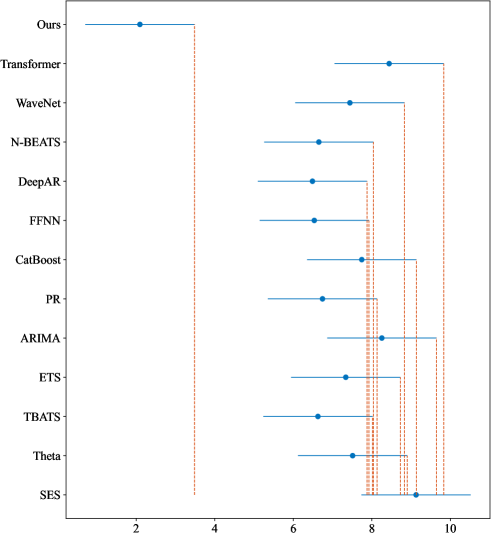
(a)     MAE Comparison Among Models Without ^∗

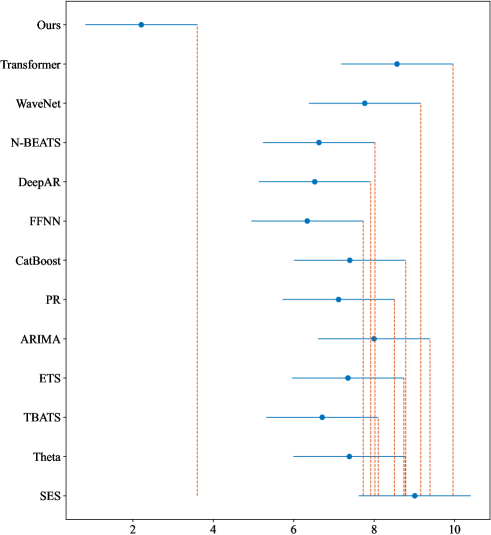
(b)     RMSE Comparison Among Models Without ^∗

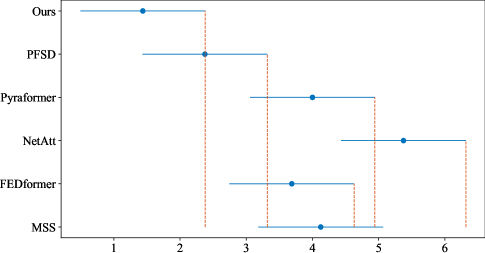
(c)     MAE Comparison Among Models With ^∗

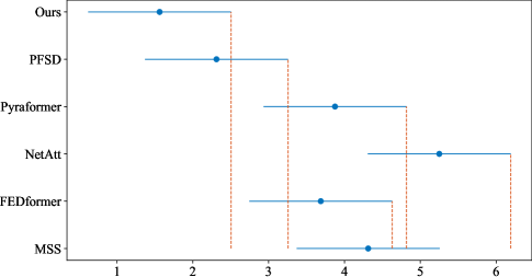
(d)     RMSE Comparison Among Models With ^∗

Figure 3: Friedman Test Figure: the Performance Comparison Based MAE and RMSE Among Models From the Perspective of Nemenyi Test.

4.4 Implementation Details

The proposed model is realized using the code framework provided by Pytorch 1.13.0. The experimental is conducted with CPU AMD 5900X, GPU NVIDIA RTX 3090, 64GB memory and SSD 2TB. The model is trained for 500 epochs using optimizer NAdam, scheduler ReduceLROnPlateau with factor 0.5, eps 1e-5, threshold 1e-5 and patience 5 and loss function L1Loss without any data augmentation.

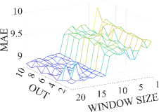
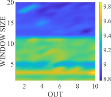
(a) Saugeenday Dataset

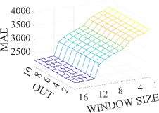
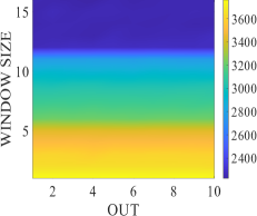
(b) Tourism Monthly Dataset

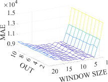
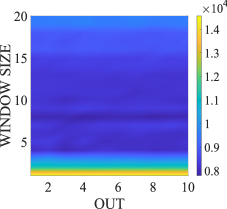
(c) Tourism Quarterly Dataset

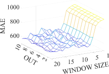
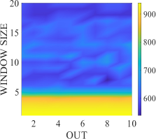
(d) US Births Dataset

Figure 4: MAE Variations When Parameter OUT and Window Size Vary on Univariate Datasets

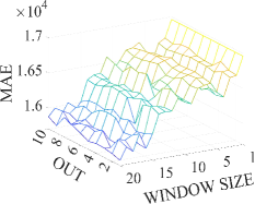
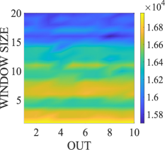
(a) Electricity Weekly Dataset

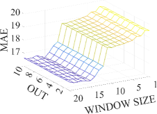
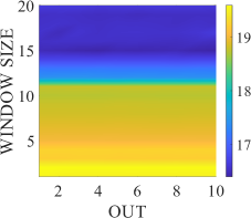
(b) Hospital Dataset

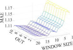
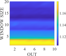
(c) Traffic Weekly Dataset

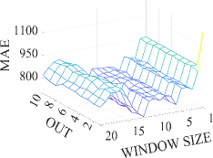
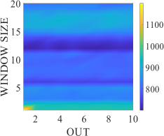
(d) Solar Weekly Dataset

Figure 5: MAE Variations When Parameter OUT and Window Size Vary on Multivariate Datasets

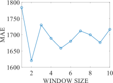
(a) M1 Monthly Dataset

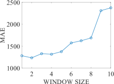
(b) M1 Quarterly Dataset

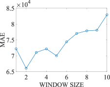
(c) M1 Yearly Dataset

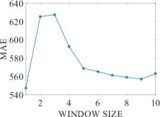
(d) M3 Monthly Dataset

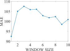
(e) M3 Other Dataset

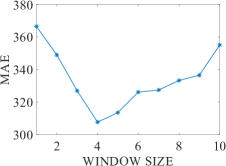
(f) M3 Quarterly Dataset

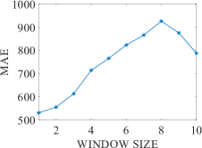
(g) M3 Yearly Dataset

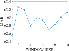
(h) M4 Daily Dataset

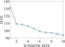
(i) M4 Hourly Dataset

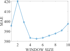
(j) M4 Quarterly Dataset

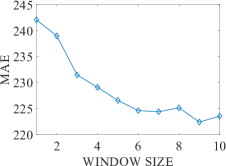
(k) M4 Weekly Dataset

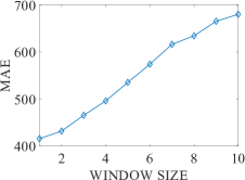
(l) M4 Yearly Dataset

Figure 6: MAE Variations on Different Window Sizes on Univariate Datasets

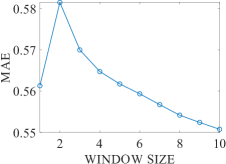
(a) Car Parts Dataset

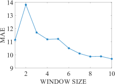
(b) Covid Deaths Dataset

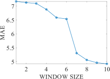
(c) NN5 Daily Dataset

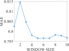
(d) Rideshare Dataset

Figure 7: MAE Variations on Different Window Sizes on Multivariate Datasets

4.5 Discussion on Experimental Results

The experimental results of univariate and multivariate datasets are provided in Table I, II and Table III, IV respectively. Generally, the proposed model obtains state-of-the-art results on most of the experimental time series datasets. However, the results of RMSE fail to remain consistent with MAE, it demonstrates that the proposed model’s ability in handling abnormal prediction values is relatively lacking. We argue that the main reason for this phenomenon is that the proposed model pays much more attention to the global information distributed to the elements captured by the sliding window and ignores the influence of the original values on the future trend to a certain extent due to the strategies of data encoding and utilization of information processed of the proposed model. Especially, our proposed model outperforms transformer-based methods which attract lots of researchers’ attention recently on almost all of the datasets, we consider that temporal data is not similar to images and videos in which there are enormous amount of semantic information needed to be extracted .

4.6 Overall Performance Comparison Between Proposed and Comparative Models

In order to comprehensively demonstrate superiority of the proposed model, we utilize Nemenyi test with $CD=q_{0.05}\sqrt{\frac{k(k+1)}{6N_{d}}}$ in which $k$ is the number of algorithms participating in the comparison and $N$is the number of datasets. Due to lack of some results of models with superscript $*$ on certain datasets, the Nemenyi test is divided into two groups to ensure fairness of comparison and the evaluation results are shown in Friedman test figure at Fig.3. It can be easily concluded that the proposed model acquire the most excellent integrated performance on experimental datasets provided.

4.7 Parameter Study

Different datasets have their corresponding optimal parameter setting for the proposed model. We selected four univariate and four multivariate data sets for a brief analysis. In Fig.4 and 5, it can be obtained that the performance of the proposed model benefits from a larger window size. And lifting factor $OUT$ has limited influence on the model capability and can reduce the error in some cases. Besides, synthesizing conditions of Fig.6 and 7, increasing the window size dose not necessarily improve model’s performance, but larger window sizes can help capture more information and establish the foundation of precise predictions in general. Specifically, on multiple datasets such as M4 Monthly, Quarterly, KDD Cup 2018 and Covid Deaths datasets, error increases considerably when window size equals 2. The main reason probably is that the size sacrifices timeliness of data to some extent and is not capable of providing sufficient semantic information to the model so that the proposed model encounters difficulty in producing accurate predictions.

Figure 8: Qualitative Prediction Results by the Proposed Method on Aus. Electricity Demand Dataset

5 Conclusion

In this paper, a novel time series forecasting model is proposed which consists of encoder part and semi-asymmetric convolutional architecture. The main role of devised data encoder is assigning elements in original observation time series with positional information so that the model could possess a global view on observation sequences. Based on processed data, a novel architecture is designed referencing asymmetric convolution and considering variability of time series which enables the model to obtain information at flexible scales on different time series. Capturing features with separate range helps model to learn underlying relationship among elements with effective understanding of associated positional information. Both of them contributes to the outstanding performance of the proposed model.

To comprehensively demonstrate the performance of the model proposed in this paper, we conduct experiments on 27 univariate and 16 multivariate datasets. The experimental results illustrate that the proposed model outperforms comparative methods on most of forecasting tasks. Specifically, the proposed model achieves the highest rank on all competition datasets such as M series, KDD Cup and Web Traffic. In addition to these intuitive results, Nemenyi test also strongly demonstrates the excellent performance of the proposed model. Besides, we also investigate the influences of the two main parameters on 24 datasets to further explain settings of the proposed model.

Nevertheless, the proposed model achieves relatively satisfying performance in most of forecasting experiments, there are still some potentials in it which can be further explored. We think we may be able to improve the model in two possible directions: 1): The attention mechanism can be introduced into the model to help the model better understand semantic information in time series, 2): A recurrent architecture of convolutional neural network is expected to be developed to better memory past information.

References

- [1] R. R. Sharma, M. Kumar, S. Maheshwari, and K. P. Ray, “Evdhm-arima-based time series forecasting model and its application for COVID-19 cases,” IEEE Trans. Instrum. Meas., vol. 70, pp. 1–10, 2021.
- [2] Q. Tan, M. Ye, A. J. Ma, B. Yang, T. C. Yip, G. L. Wong, and P. C. Yuen, “Explainable uncertainty-aware convolutional recurrent neural network for irregular medical time series,” IEEE Trans. Neural Networks Learn. Syst., vol. 32, no. 10, pp. 4665–4679, 2021.
- [3] D. Cheng, F. Yang, S. Xiang, and J. Liu, “Financial time series forecasting with multi-modality graph neural network,” Pattern Recognit., vol. 121, p. 108218, 2022.
- [4] G. Liu, F. Xiao, C. Lin, and Z. Cao, “A fuzzy interval time-series energy and financial forecasting model using network-based multiple time-frequency spaces and the induced-ordered weighted averaging aggregation operation,” IEEE Trans. Fuzzy Syst., vol. 28, no. 11, pp. 2677–2690, 2020.
- [5] E. Uchiteleva, S. Primak, M. Luccini, A. R. Hussein, and A. Shami, “The trils approach for drift-aware time-series prediction in iiot environment,” IEEE Trans. Ind. Informatics, vol. 18, no. 10, pp. 6581–6591, 2022.
- [6] T. Zhou, Z. Ma, Q. Wen, X. Wang, L. Sun, and R. Jin, “Fedformer: Frequency enhanced decomposed transformer for long-term series forecasting,” arXiv preprint arXiv:2201.12740, 2022.
- [7] S. Liu, H. Yu, C. Liao, J. Li, W. Lin, A. X. Liu, and S. Dustdar, “Pyraformer: Low-complexity pyramidal attention for long-range time series modeling and forecasting,” in The Tenth International Conference on Learning Representations, ICLR 2022, Virtual Event, April 25-29, 2022. OpenReview.net, 2022.
- [8] H. Zhou, S. Zhang, J. Peng, S. Zhang, J. Li, H. Xiong, and W. Zhang, “Informer: Beyond efficient transformer for long sequence time-series forecasting,” in Proceedings of the AAAI Conference on Artificial Intelligence, vol. 35, no. 12, 2021, pp. 11 106–11 115.
- [9] M. Chen, H. Peng, J. Fu, and H. Ling, “Autoformer: Searching transformers for visual recognition,” in 2021 IEEE/CVF International Conference on Computer Vision, ICCV 2021, Montreal, QC, Canada, October 10-17, 2021. IEEE, 2021, pp. 12 250–12 260.
- [10] A. Zeng, M. Chen, L. Zhang, and Q. Xu, “Are transformers effective for time series forecasting?” CoRR, vol. abs/2205.13504, 2022.
- [11] Y. He, L. Li, X. Zhu, and K. L. Tsui, “Multi-graph convolutional-recurrent neural network (MGC-RNN) for short-term forecasting of transit passenger flow,” IEEE Trans. Intell. Transp. Syst., vol. 23, no. 10, pp. 18 155–18 174, 2022.
- [12] Y. Liu, C. Gong, L. Yang, and Y. Chen, “DSTP-RNN: A dual-stage two-phase attention-based recurrent neural network for long-term and multivariate time series prediction,” Expert Syst. Appl., vol. 143, 2020.
- [13] D. K. Dennis, D. A. E. Acar, V. Mandikal, V. S. Sadasivan, V. Saligrama, H. V. Simhadri, and P. Jain, “Shallow RNN: accurate time-series classification on resource constrained devices,” in Advances in Neural Information Processing Systems 32: Annual Conference on Neural Information Processing Systems 2019, NeurIPS 2019, December 8-14, 2019, Vancouver, BC, Canada, 2019, pp. 12 896–12 906.
- [14] K. Guo, N. Wang, D. Liu, and X. Peng, “Uncertainty-aware LSTM based dynamic flight fault detection for UAV actuator,” IEEE Trans. Instrum. Meas., vol. 72, pp. 1–13, 2023.
- [15] Y. Tang, F. Yu, W. Pedrycz, X. Yang, J. Wang, and S. Liu, “Building trend fuzzy granulation-based LSTM recurrent neural network for long-term time-series forecasting,” IEEE Trans. Fuzzy Syst., vol. 30, no. 6, pp. 1599–1613, 2022.
- [16] K. Bandara, C. Bergmeir, and H. Hewamalage, “Lstm-msnet: Leveraging forecasts on sets of related time series with multiple seasonal patterns,” IEEE Trans. Neural Networks Learn. Syst., vol. 32, no. 4, pp. 1586–1599, 2021.
- [17] V. L. Guen and N. Thome, “Deep time series forecasting with shape and temporal criteria,” IEEE Trans. Pattern Anal. Mach. Intell., vol. 45, no. 1, pp. 342–355, 2023.
- [18] Y. Li, K. Li, C. Chen, X. Zhou, Z. Zeng, and K. Li, “Modeling temporal patterns with dilated convolutions for time-series forecasting,” ACM Trans. Knowl. Discov. Data, vol. 16, no. 1, pp. 14:1–14:22, 2022.
- [19] Y. Chen, I. Segovia-Dominguez, B. Coskunuzer, and Y. R. Gel, “Tamp-s2gcnets: Coupling time-aware multipersistence knowledge representation with spatio-supra graph convolutional networks for time-series forecasting,” in The Tenth International Conference on Learning Representations, ICLR 2022, Virtual Event, April 25-29, 2022. OpenReview.net, 2022.
- [20] S. Bai, J. Z. Kolter, and V. Koltun, “An empirical evaluation of generic convolutional and recurrent networks for sequence modeling,” CoRR, vol. abs/1803.01271, 2018.
- [21] G. Liu, “Time series forecasting via learning convolutionally low-rank models,” IEEE Trans. Inf. Theory, vol. 68, no. 5, pp. 3362–3380, 2022.
- [22] S. Liu, H. Ji, and M. C. Wang, “Nonpooling convolutional neural network forecasting for seasonal time series with trends,” IEEE Trans. Neural Networks Learn. Syst., vol. 31, no. 8, pp. 2879–2888, 2020.
- [23] Y. Li, H. Wang, J. Li, C. Liu, and J. Tan, “ACT: adversarial convolutional transformer for time series forecasting,” in International Joint Conference on Neural Networks, IJCNN 2022, Padua, Italy, July 18-23, 2022. IEEE, 2022, pp. 1–8.
- [24] P. Fergus, C. Chalmers, C. A. C. Montañez, D. Reilly, P. Lisboa, and B. Pineles, “Modelling segmented cardiotocography time-series signals using one-dimensional convolutional neural networks for the early detection of abnormal birth outcomes,” IEEE Trans. Emerg. Top. Comput. Intell., vol. 5, no. 6, pp. 882–892, 2021.
- [25] Y. Wang, Z. Liu, D. Hu, and M. Zhang, “Multivariate time series prediction based on optimized temporal convolutional networks with stacked auto-encoders,” in Proceedings of The 11th Asian Conference on Machine Learning, ACML 2019, 17-19 November 2019, Nagoya, Japan. PMLR, 2019, pp. 157–172.
- [26] S. Chen, “Forecasting enrollments based on fuzzy time series,” Fuzzy Sets Syst., vol. 81, no. 3, pp. 311–319, 1996.
- [27] Q. Ma, Z. Chen, S. Tian, and W. W. Y. Ng, “Difference-guided representation learning network for multivariate time-series classification,” IEEE Trans. Cybern., vol. 52, no. 6, pp. 4717–4727, 2022.
- [28] H. Zhang, Z. Tang, Y. Xie, H. Yuan, Q. Chen, and W. Gui, “Siamese time series and difference networks for performance monitoring in the froth flotation process,” IEEE Trans. Ind. Informatics, vol. 18, no. 4, pp. 2539–2549, 2022.
- [29] K. Gao, W. Feng, X. Zhao, C. Yu, W. Su, Y. Niu, and L. Han, “Anomaly detection for time series with difference rate sample entropy and generative adversarial networks,” Complex., vol. 2021, pp. 5 854 096:1–5 854 096:13, 2021.
- [30] X. Wang, H. Zhang, Y. Zhang, M. Wang, J. Song, T. Lai, and M. Khushi, “Learning nonstationary time-series with dynamic pattern extractions,” IEEE Trans. Artif. Intell., vol. 3, no. 5, pp. 778–787, 2022.
- [31] J. Jin, A. Dundar, and E. Culurciello, “Flattened convolutional neural networks for feedforward acceleration,” in 3rd International Conference on Learning Representations, ICLR 2015, San Diego, CA, USA, May 7-9, 2015, Workshop Track Proceedings, 2015.
- [32] S. Lo, H. Hang, S. Chan, and J. Lin, “Efficient dense modules of asymmetric convolution for real-time semantic segmentation,” in MMAsia ’19: ACM Multimedia Asia, Beijing, China, December 16-18, 2019. ACM, 2019, pp. 1:1–1:6.
- [33] J. Ye, Z. Liu, B. Du, L. Sun, W. Li, Y. Fu, and H. Xiong, “Learning the evolutionary and multi-scale graph structure for multivariate time series forecasting,” in KDD ’22: The 28th ACM SIGKDD Conference on Knowledge Discovery and Data Mining, Washington, DC, USA, August 14 - 18, 2022, A. Zhang and H. Rangwala, Eds. ACM, 2022, pp. 2296–2306.
- [34] P. Meschenmoser, J. F. Buchmüller, D. Seebacher, M. Wikelski, and D. A. Keim, “Multisegva: Using visual analytics to segment biologging time series on multiple scales,” IEEE Trans. Vis. Comput. Graph., vol. 27, no. 2, pp. 1623–1633, 2021.
- [35] M. Jaderberg, A. Vedaldi, and A. Zisserman, “Speeding up convolutional neural networks with low rank expansions,” in British Machine Vision Conference, BMVC 2014, Nottingham, UK, September 1-5, 2014. BMVA Press, 2014.
- [36] F. Liu, X. Zhou, J. Cao, Z. Wang, T. Wang, H. Wang, and Y. Zhang, “Anomaly detection in quasi-periodic time series based on automatic data segmentation and attentional LSTM-CNN,” IEEE Trans. Knowl. Data Eng., vol. 34, no. 6, pp. 2626–2640, 2022.
- [37] Y. Oh, “Multivariate times series classification using multichannel CNN,” in Proceedings of the Thirty-First International Joint Conference on Artificial Intelligence, IJCAI 2022, Vienna, Austria, 23-29 July 2022. ijcai.org, 2022, pp. 5865–5866.
- [38] X. Ding, X. Zhang, N. Ma, J. Han, G. Ding, and J. Sun, “Repvgg: Making vgg-style convnets great again,” in IEEE Conference on Computer Vision and Pattern Recognition, CVPR 2021, virtual, June 19-25, 2021. Computer Vision Foundation / IEEE, 2021, pp. 13 733–13 742.
- [39] E. L. Denton, W. Zaremba, J. Bruna, Y. LeCun, and R. Fergus, “Exploiting linear structure within convolutional networks for efficient evaluation,” in Advances in Neural Information Processing Systems 27: Annual Conference on Neural Information Processing Systems 2014, December 8-13 2014, Montreal, Quebec, Canada, 2014, pp. 1269–1277.
- [40] X. Ding, Y. Guo, G. Ding, and J. Han, “Acnet: Strengthening the kernel skeletons for powerful CNN via asymmetric convolution blocks,” in 2019 IEEE/CVF International Conference on Computer Vision, ICCV 2019, Seoul, Korea (South), October 27 - November 2, 2019. IEEE, 2019, pp. 1911–1920.
- [41] A. Paszke, A. Chaurasia, S. Kim, and E. Culurciello, “Enet: A deep neural network architecture for real-time semantic segmentation,” CoRR, vol. abs/1606.02147, 2016.
- [42] L. Chen, G. Papandreou, I. Kokkinos, K. Murphy, and A. L. Yuille, “Semantic image segmentation with deep convolutional nets and fully connected crfs,” in 3rd International Conference on Learning Representations, ICLR 2015, San Diego, CA, USA, May 7-9, 2015, Conference Track Proceedings, 2015.
- [43] L. Chen, G. Papandreou, I. Kokkinos, K. Murphy, and A. L. Yuille, “Deeplab: Semantic image segmentation with deep convolutional nets, atrous convolution, and fully connected crfs,” IEEE Trans. Pattern Anal. Mach. Intell., vol. 40, no. 4, pp. 834–848, 2018.
- [44] A. van den Oord, S. Dieleman, H. Zen, K. Simonyan, O. Vinyals, A. Graves, N. Kalchbrenner, A. W. Senior, and K. Kavukcuoglu, “Wavenet: A generative model for raw audio,” p. 125, 2016.
- [45] Q. Song and B. Chissom, “Fuzzy time series and its model,” Fuzzy Sets and Systems, vol. 54, p. 269–277, 03 1993.
- [46] L. A. Zadeh, “Fuzzy sets,” Inf. Control., vol. 8, no. 3, pp. 338–353, 1965.
- [47] Q. Song and B. Chissom, “Forecasting enrollments with fuzzy time series—part ii,” Fuzzy Sets and Systems, vol. 62, pp. 1–8, 02 1994.
- [48] R. Godahewa, C. Bergmeir, G. I. Webb, R. J. Hyndman, and P. Montero-Manso, “Monash time series forecasting archive,” in Proceedings of the Neural Information Processing Systems Track on Datasets and Benchmarks 1, NeurIPS Datasets and Benchmarks 2021, December 2021, virtual, 2021.
- [49] C. Holt, “Forecasting trends and seasonal by exponentially weighted averages,” Office of Naval Research Memorandum, vol. 20, 01 1957.
- [50] V. Assimakopoulos and K. Nikolopoulos, “The theta model: A decomposition approach to forecasting,” International Journal of Forecasting, vol. 16, pp. 521–530, 10 2000.
- [51] A. De Livera, R. Hyndman, and R. Snyder, “Forecasting time series with complex seasonal patterns using exponential smoothing,” Journal of the American Statistical Association, vol. 106, pp. 1513–1527, 01 2010.
- [52] R. Hyndman, A. Koehler, K. Ord, and R. Snyder, “Forecasting with exponential smoothing. the state space approach,” 01 2008.
- [53] B. Box, G. Jenkins, G. Reinsel, and G. Ljung, Time Series Analysis: Forecasting and Control, 01 2016, vol. 68.
- [54] R. J. Hyndman and G. Athanasopoulos, Forecasting: principles and practice. OTexts, 2018.
- [55] J. R. Trapero, N. Kourentzes, and R. Fildes, “On the identification of sales forecasting models in the presence of promotions,” J. Oper. Res. Soc., vol. 66, no. 2, pp. 299–307, 2015.
- [56] L. O. Prokhorenkova, G. Gusev, A. Vorobev, A. V. Dorogush, and A. Gulin, “Catboost: unbiased boosting with categorical features,” in Advances in Neural Information Processing Systems 31: Annual Conference on Neural Information Processing Systems 2018, NeurIPS 2018, December 3-8, 2018, Montréal, Canada, 2018, pp. 6639–6649.
- [57] I. Goodfellow, Y. Bengio, and A. Courville, Deep Learning. MIT Press, 2016, http://www.deeplearningbook.org.
- [58] V. Flunkert, D. Salinas, and J. Gasthaus, “Deepar: Probabilistic forecasting with autoregressive recurrent networks,” International Journal of Forecasting, vol. 36, 04 2017.
- [59] B. N. Oreshkin, D. Carpov, N. Chapados, and Y. Bengio, “N-BEATS: neural basis expansion analysis for interpretable time series forecasting,” in 8th International Conference on Learning Representations, ICLR 2020, Addis Ababa, Ethiopia, April 26-30, 2020. OpenReview.net, 2020.
- [60] A. Borovykh, S. Bohte, and C. W. Oosterlee, “Conditional time series forecasting with convolutional neural networks,” arXiv preprint arXiv:1703.04691, 2017.
- [61] A. Vaswani, N. Shazeer, N. Parmar, J. Uszkoreit, L. Jones, A. N. Gomez, L. Kaiser, and I. Polosukhin, “Attention is all you need,” in Advances in Neural Information Processing Systems 30: Annual Conference on Neural Information Processing Systems 2017, December 4-9, 2017, Long Beach, CA, USA, 2017, pp. 5998–6008.
- [62] Y. Hu and F. Xiao, “An efficient forecasting method for time series based on visibility graph and multi-subgraph similarity,” Chaos, Solitons & Fractals, vol. 160, p. 112243, 07 2022.
- [63] Y. Hu and F. Xiao, “Network self attention for forecasting time series,” Appl. Soft Comput., vol. 124, p. 109092, 2022.
- [64] Y. Hu and F. Xiao, “Time series forecasting based on fuzzy cognitive visibility graph and weighted multi-subgraph similarity,” IEEE Transactions on Fuzzy Systems, 2022.