An Efficient Solution to s-Rectangular Robust Markov Decision Processes

Navdeep Kumar Technion Kfir Levy Technion Kaixin Wang National University of Singapore Shie Mannor Technion
Abstract

We present an efficient robust value iteration for s-rectangular robust Markov Decision Processes (MDPs) with a time complexity comparable to standard (non-robust) MDPs which is significantly faster than any existing method. We do so by deriving the optimal robust Bellman operator in concrete forms using our $L_{p}$ water filling lemma. We unveil the exact form of the optimal policies, which turn out to be novel threshold policies with the probability of playing an action proportional to its advantage.

1 Introduction

In Markov Decision Processes (MDPs), an agent interacts with the environment and learns to optimally behave in it ย [28]. However, the MDP solution may be very sensitive to little changes in the model parameters ย [23]. Hence we should be cautious applying the solution of the MDP, when the model is changing or when there is uncertainty in the model parameters. Robust MDPs provide a way to address this issue, where an agent can learn to optimally behave even when the model parameters are uncertain ย [15, 29, 18]. Another motivation to study robust MDPs is that they can lead to better generalization [33, 34, 25] compared to non-robust solutions.

Unfortunately, solving robust MDPs is proven to be NP-hard for general uncertainty sets [32]. As a result, the uncertainty set is often assumed to be rectangular, which enables the existence of a contractive robust Bellman operators to obtain the optimal robust value function [24, 18, 22, 12, 32]. Recently, there has been progress in solving robust MDPs for some sa-rectangular uncertainty sets via both value-based and policy-based methods [30, 31]. An uncertainty set is said to be sa-rectangular if it can be expressed as a Cartesian product of the uncertainty in all states and actions. It can be further generalized to a s-rectangular uncertainty set if it can be expressed as a Cartesian product of the uncertainty in all states only. Compared to sa-rectangular robust MDPs, s-rectangular robust MDPs are less conservative and hence more desirable; however, they are also much more difficult and poorly understood [32]. Currently, there are few works that consider s-rectangular $L_{p}$ robust MDPs where uncertainty set is further constrained by $L_{p}$ norm, but they rely on black box methods which limits its applicability and offers little insights [7, 16, 9, 32]. No effective value or policy based methods exist for solving any s-robust MDPs. Moreover, it is known that optimal policies in s-rectangular robust MDPs can be stochastic, in contrast to sa-rectangular robust MDPs and non-robust MDPs [32]. However, so far, nothing is known about the stochastic nature of the optimal policies in s-rectangular MDPs.

In this work, we mainly focus on s-rectangular $L_{p}$ robust MDPs. We first revise the unrealistic assumptions made in the noise transition kernel in [9] and introduce forbidden transitions, which leads to novel regularizers. Then we derive robust Bellman operator (policy evaluation) for a s-rectangular robust MDPs in closed form which is equivalent to reward-value-policy-regularized non-robust Bellman operator without radius assumption 5.1 in [9]. We exploit this equivalence to derive an optimal robust Bellman operator in concrete forms using our $L_{p}$-water pouring lemma which generalizes existing water pouring lemma for $L_{2}$ case [1]. We can compute these operators in closed form for $p=1,\infty$ and exactly by a simple algorithm for $p=2$, and approximately by binary search for general $p$. We show that the time complexity of robust value iteration for $p=1,2$ is the same as that of non-robust value iteration. For general $p$, the complexity includes some additional log-factors due to binary searches.

In addition, we derive a complete characterization of the stochastic nature of optimal policies in s-rectangular robust MDPs. The optimal policies in this case, are threshold policies, that plays only actions with positive advantage with probability proportional to $(p-1)$-th power to its advantage.

Related Work. For sa-rectangular R-contamination robust MDPs, [30] derived robust Bellman operators which are equivalent to value-regularized-non-robust Bellman operators, enabling efficient robust value iteration. Building upon this work, [31] derived robust policy gradient which is equivalvent to non-robust policy gradient with regularizer and correction terms. Unfortunately, these methods canโ€™t be naturally generalized to s-rectangular robust MDPs.

For s-rectangular robust MDPs, methods such as robust value iteration [6, 32], robust modified policy iteration [19], partial robust policy iteration [16] etc tries to approximately evaluate robust Bellman operators using variety of tools to estimate optimal robust value function. The scalability of these methods has been limited due to their reliance on an external black-box solver such as Linear Programming.

Previous works have explored robust MDPs from a regularization perspective [9, 10, 17, 11]. Specifically, [9] showed that s-rectangular robust MDPs is equivalent to reward-value-policy regularized MDPs, and proposed a gradient based policy iteration for s-rectangular $L_{p}$ robust MDPs ( where uncertainty set is s-rectangular and constrained by $L_{p}$ norm). But this gradient based policy improvement relies on black box simplex projection, hence very slow and not scalable.

The detailed discussion of the above works can be found in the appendix.

2 Preliminary

2.1 Notations

For a set $\mathcal{S}$, $\lvert\mathcal{S}\rvert$ denotes its cardinality. โŸจu,vโŸฉ:=โˆ‘sโˆˆ๐’ฎuโ€‹(s)โ€‹vโ€‹(s)assign๐‘ข๐‘ฃsubscript๐‘ ๐’ฎ๐‘ข๐‘ ๐‘ฃ๐‘ \langle u,v\rangle:=\sum_{s\in\mathcal{S}}u(s)v(s) denotes the dot product between functions $u,v:\mathcal{S}\to\mathbb{R}$. โˆฅvโˆฅpq:=(โˆ‘s|vโ€‹(s)|p)qpassignsuperscriptsubscriptdelimited-โˆฅโˆฅ๐‘ฃ๐‘๐‘žsuperscriptsubscript๐‘ superscript๐‘ฃ๐‘ ๐‘๐‘ž๐‘\lVert v\rVert_{p}^{q}:=(\sum_{s}\lvert v(s)\rvert^{p})^{\frac{q}{p}} denotes the $q$-th power of $L_{p}$ norm of function $v$, and we use $\lVert v\rVert_{p}:=\lVert v\rVert^{1}_{p}$ and $\lVert v\rVert:=\lVert v\rVert_{2}$ as shorthand. For a set $\mathcal{C}$, $\Delta_{\mathcal{C}}:=\{a:\mathcal{C}\to\mathbb{R}|a(c)\geq 0,\forall c,\sum_{c\in\mathcal{C}}a_{c}=1\}$ is the probability simplex over $\mathcal{C}$. $\mathbf{0},\mathbf{1}$ denotes all zero vector and all ones vector/function respectively of appropriate dimension/domain. $\mathbf{1}(a=b):=1$ if $a=b$, 0 otherwise, is the indicator function. For vectors $u,v$, $\mathbf{1}(u\geq v)$ is component wise indicator vector, i.e. $\mathbf{1}(u\geq v)(x)=\mathbf{1}(u(x)\geq v(x))$. $A\times B=\{(a,b)\mid a\in A,b\in B\}$ is cartesain product between set $A$ and $B$.

2.2 Markov Decision Processes

A Markov Decision Process (MDP) can be described as a tuple $(\mathcal{S},\mathcal{A},P,R,\gamma,\mu)$, where $\mathcal{S}$ is the state space, $\mathcal{A}$ is the action space, $P$ is a transition kernel mapping $\mathcal{S}\times\mathcal{A}$ to $\Delta_{\mathcal{S}}$, $R$ is a reward function mapping $\mathcal{S}\times\mathcal{A}$ to $\mathbb{R}$, $\mu$ is an initial distribution over states in $\mathcal{S}$, and $\gamma$ is a discount factor in $[0,1)$. The expected discounted cumulative reward (return) is defined as

$\displaystyle\rho^{\pi}_{(P,R)}:=$ $\displaystyle\mathbb{E}\left[\sum_{n=0}^{\infty}\gamma^{n}R(s_{n},a_{n})\Bigm{|}s_{0}\sim\mu,\pi,P\right].$

The return can be written compactly as

$\displaystyle\rho^{\pi}_{(P,R)}=\langle\mu,v^{\pi}_{(P,R)}\rangle,$ (1)

[26] where $v^{\pi}_{(P,R)}$ is the value function , defined as

$\displaystyle v^{\pi}_{(P,R)}(s):=\mathbb{E}\left[\sum_{n=0}^{\infty}\gamma^{n}R(s_{n},a_{n})\Bigm{|}s_{0}=s,\pi,P\right].$ (2)

Our objective is to find an optimal policy $\pi^{*}_{(P,R)}$ that maximizes the performance $\rho^{\pi}_{(P,R)}$. This performance can be written as :

$\displaystyle\rho^{*}_{(P,R)}:=\max_{\pi}\rho^{\pi}_{(P,R)}=\langle\mu,v^{*}_{(P,R)}\rangle,$ (3)

where $v^{*}_{(P,R)}:=\max_{\pi}v^{\pi}_{(P,R)}$ is the optimal value function [26].

The value function $v^{\pi}_{(P,R)}$ and the optimal value function $v^{*}_{(P,R)}$ are the fixed points of the Bellman operator $\mathcal{T}^{\pi}_{(P,R)}$ and the robust Bellman operator $\mathcal{T}^{*}_{(P,R)}$, respectively [28]. These $\gamma$-contraction operators are defined as follows: For any vector $v$, and state sโˆˆ๐’ฎ๐‘ ๐’ฎs\in\mathcal{S},

(๐’ฏ(P,R)ฯ€โ€‹v)โ€‹(s)subscriptsuperscript๐’ฏ๐œ‹๐‘ƒ๐‘…๐‘ฃ๐‘ \displaystyle(\mathcal{T}^{\pi}_{(P,R)}v)(s) $\displaystyle:=\sum_{a}\pi(a|s)\Bigm{[}R(s,a)+\gamma\sum_{s^{\prime}}P(s^{\prime}|s,a)v(s^{\prime})\Bigm{]},\quad\text{and}$
$\displaystyle\mathcal{T}^{*}_{(P,R)}v$ $\displaystyle:=\max_{\pi}\mathcal{T}^{\pi}_{(P,R)}v.$

Therefore, the value iteration $v_{n+1}:=\mathcal{T}^{*}_{(P,R)}v_{n}$ converges linearly to the optimal value function $v^{*}_{(P,R)}$. Given this optimal value function, the optimal policy can be computed as: $\pi^{*}_{(P,R)}\in\text{arg}\max_{\pi}\mathcal{T}^{\pi}_{(P,R)}v^{*}_{(P,R)}$.

Remark 1.

The vector minimum of a set $U$ of vectors is defined component wise, i.e. $(\min_{u\in U}u)(i):=\min_{u\in U}u(i)$. This operation is well-defined only when there exists a minimal vector $u^{*}\in U$ such that $u^{*}\preceq u,\forall u\in U$. The same holds for other operations such as maximum, argmin, argmax, etc.

2.3 Robust Markov Decision Processes

A robust Markov Decision Process (MDP) is a tuple $(\mathcal{S},\mathcal{A},\mathcal{P},\mathcal{R},\gamma,\mu)$ which generalizes the standard MDP by containing a set of transition kernels $\mathcal{P}$ and set of reward functions $\mathcal{R}$. Let uncertainty set $\mathcal{U}=\mathcal{P}\times\mathcal{R}$ be set of tuples of transition kernels and reward functions [18, 24]. The robust performance $\rho^{\pi}_{\mathcal{U}}$ of a policy $\pi$ is defined to be its worst performance on the entire uncertainty set $\mathcal{U}$ as

$\displaystyle\rho^{\pi}_{\mathcal{U}}:=\min_{(P,R)\in\mathcal{U}}\rho^{\pi}_{(P,R)}.$ (4)

Our objective is to find an optimal robust policy $\pi^{*}_{\mathcal{U}}$ that maximizes the robust performance $\rho^{\pi}_{\mathcal{U}}$, defined as

$\displaystyle\rho^{*}_{\mathcal{U}}:=\max_{\pi}\rho^{\pi}_{\mathcal{U}}.$ (5)

Solving the above robust objectives 4 and 5 are strongly NP-hard for general uncertainty sets, even if they are convex [32]. Hence, the uncertainty set $\mathcal{U}=\mathcal{P}\times\mathcal{R}$ is commonly assumed to be s-rectangular, meaning that $\mathcal{R}$ and $\mathcal{P}$ can be decomposed state-wise as $\mathcal{R}=\times_{s\in\mathcal{S}}\mathcal{R}_{s}$ and $\mathcal{P}=\times_{s\in\mathcal{S}}\mathcal{P}_{s}$. For further simplification, $\mathcal{U}=\mathcal{P}\times\mathcal{R}$ is assumed to decompose state-action-wise as $\mathcal{R}=\times_{(s,a)\in\mathcal{S}\times\mathcal{A}}\mathcal{R}_{s,a}$ and $\mathcal{P}=\times_{(s,a)\in\mathcal{S}\times\mathcal{A}}\mathcal{P}_{s,a}$, known as sa-rectangular uncertainty set. Throughout the paper, the uncertainty set is assumed to be s-rectangular (or sa-rectangular) unless stated otherwise. Under the s-rectangularity assumption, for every policy $\pi$, there exists a robust value function $v^{\pi}_{\mathcal{U}}$ which is the minimum of $v^{\pi}_{(P,R)}$ for all $(P,R)\in\mathcal{U}$, and the optimal robust value function $v^{*}_{\mathcal{U}}$ which is the maximum of $v^{\pi}_{\mathcal{U}}$ for all policies $\pi$ [32], that is

$$v^{\pi}_{\mathcal{U}}:=\min_{{(P,R)\in\mathcal{U}}}v^{\pi}_{(P,R)},\quad\text{and}\quad v^{*}_{\mathcal{U}}:=\max_{\pi}v^{\pi}_{\mathcal{U}}.$$

This implies, robust policy performance can be rewritten as

$\displaystyle\rho^{\pi}_{\mathcal{U}}=\langle\mu,v^{\pi}_{\mathcal{U}}\rangle,\quad\text{and}\quad\rho^{*}_{\mathcal{U}}=\langle\mu,v^{*}_{\mathcal{U}}\rangle.$

Furthermore, the robust value function $v^{\pi}_{\mathcal{U}}$ is the fixed point of the robust Bellmen operator $\mathcal{T}^{\pi}_{\mathcal{U}}$ [32, 18], defined as

(๐’ฏ๐’ฐฯ€โ€‹v)โ€‹(s):=min(P,R)โˆˆ๐’ฐโ€‹โˆ‘aฯ€โ€‹(a|s)โ€‹[Rโ€‹(s,a)+ฮณโ€‹โˆ‘sโ€ฒPโ€‹(sโ€ฒ|s,a)โ€‹vโ€‹(sโ€ฒ)],assignsubscriptsuperscript๐’ฏ๐œ‹๐’ฐ๐‘ฃ๐‘ subscript๐‘ƒ๐‘…๐’ฐsubscript๐‘Ž๐œ‹conditional๐‘Ž๐‘ delimited-[]๐‘…๐‘ ๐‘Ž๐›พsubscriptsuperscript๐‘ โ€ฒ๐‘ƒconditionalsuperscript๐‘ โ€ฒ๐‘ ๐‘Ž๐‘ฃsuperscript๐‘ โ€ฒ\displaystyle(\mathcal{T}^{\pi}_{\mathcal{U}}v)(s):=\min_{(P,R)\in\mathcal{U}}\sum_{a}\pi(a|s)\left[R(s,a)+\gamma\sum_{s^{\prime}}P(s^{\prime}|s,a)v(s^{\prime})\right],

and the optimal robust value function $v^{*}_{\mathcal{U}}$ is the fixed point of the optimal robust Bellman operator $\mathcal{T}^{*}_{\mathcal{U}}$ [18, 32], defined as

$\displaystyle\mathcal{T}^{*}_{\mathcal{U}}v:=\max_{\pi}\mathcal{T}^{\pi}_{\mathcal{U}}v.$

The optimal robust Bellman operator $\mathcal{T}^{*}_{\mathcal{U}}$ and robust Bellman operators $\mathcal{T}^{\pi}_{\mathcal{U}}$ are $\gamma$ contraction maps for all policy $\pi$ [32], that is

$\displaystyle\lVert\mathcal{T}^{*}_{\mathcal{U}}v-\mathcal{T}^{*}_{\mathcal{U}}u\rVert_{\infty}\leq\gamma\lVert u-v\rVert_{\infty},\qquad\lVert\mathcal{T}^{\pi}_{\mathcal{U}}v-\mathcal{T}^{\pi}_{\mathcal{U}}u\rVert_{\infty}\leq\gamma\lVert u-v\rVert_{\infty},\qquad\forall\pi,u,v.$

So for all initial values $v^{\pi}_{0},v^{*}_{0}$, sequences defined as

$\displaystyle v^{\pi}_{n+1}:=\mathcal{T}^{\pi}_{\mathcal{U}}v^{\pi}_{n},\qquad v^{*}_{n+1}:=\mathcal{T}^{*}_{\mathcal{U}}v^{*}_{n}$ (6)

converges linearly to their respective fixed points, that is $v^{\pi}_{n}\to v^{\pi}_{\mathcal{U}}$ and $v^{*}_{n}\to v^{*}_{\mathcal{U}}$. Given this optimal robust value function, the optimal robust policy can be computed as: $\pi^{*}_{\mathcal{U}}\in\text{arg}\max_{\pi}\mathcal{T}^{\pi}_{\mathcal{U}}v^{*}_{\mathcal{U}}$ [32]. This makes the robust value iteration an attractive method for solving s-rectangular robust MDPs.

3 Method

In this section, we consider constraining the uncertainty set around nominal values by the $L_{p}$ norm, which is a natural way of limiting the broad class of s (or sa)-rectangular uncertainty sets [9, 16, 3]. We will then derive robust Bellman operators for these uncertainty sets, which can be used to obtain robust value functions. This will be done separately for sa-rectangular in Subsection 3.1 and s-rectangular case in Section 3.2.

We begin by making a few useful definitions. We reserve $q$ for Holder conjugate of $p$, i.e. $\frac{1}{p}+\frac{1}{q}=1$. Let $p$-variance function $\kappa_{p}:\mathcal{S}\to\mathbb{R}$ be defined as

$$\kappa_{p}(v):=\min_{\omega\in\mathbb{R}}\lVert v-\omega\mathbf{1}\lVert_{p}.$$ (7)

For $p=1,2,\infty$, the $p$-variance function $\kappa_{p}$ has intuitive closed forms as summarized in Table 1. For general $p$, it can be calculated by binary search in the range [minsโกvโ€‹(s),maxsโกvโ€‹(s)]subscript๐‘ ๐‘ฃ๐‘ subscript๐‘ ๐‘ฃ๐‘ [\min_{s}v(s),\max_{s}v(s)] ( see appendix I for proofs).

Table 1: $p$-variance
$x$ $\kappa_{x}(v)$ Remark
$p$ $\min_{\omega\in\mathbb{R}}\lVert v-\omega\mathbf{1}\lVert_{p}$ Binary search
$\infty$ maxsโกvโ€‹(s)โˆ’minsโกvโ€‹(s)2subscript๐‘ ๐‘ฃ๐‘ subscript๐‘ ๐‘ฃ๐‘ 2\frac{\max_{s}v(s)-\min_{s}v(s)}{2} Semi-norm
$2$ $\sqrt{\sum_{s}\bigm{(}v(s)-\frac{\sum_{s}v(s)}{S}\bigm{)}^{2}}$ Variance
$1$ โˆ‘i=1โŒŠ(S+1)/2โŒ‹vโ€‹(si)superscriptsubscript๐‘–1๐‘†12๐‘ฃsubscript๐‘ ๐‘–\sum_{i=1}^{\lfloor(S+1)/2\rfloor}v(s_{i}) Top half - lower half
โˆ’โˆ‘i=โŒˆ(S+1)/2โŒ‰Svโ€‹(si)superscriptsubscript๐‘–๐‘†12๐‘†๐‘ฃsubscript๐‘ ๐‘–\quad-\sum_{i=\lceil(S+1)/2\rceil}^{S}v(s_{i})
where $v$ is sorted, i.e. vโ€‹(si)โ‰ฅvโ€‹(si+1)โˆ€i.๐‘ฃsubscript๐‘ ๐‘–๐‘ฃsubscript๐‘ ๐‘–1for-all๐‘–v(s_{i})\geq v(s_{i+1})\quad\forall i.

3.1 (Sa)-rectangular Lp robust Markov Decision Processes

In accordance with [9], we define sa-rectangular $L_{p}$ constrained uncertainty set $\mathcal{U}^{\texttt{sa}}_{p}$ as

$$\mathcal{U}^{\texttt{sa}}_{p}:=(P_{0}+\mathcal{P})\times(R_{0}+\mathcal{R})$$

where $\mathcal{P}$, $\mathcal{R}$ are noise sets around nominal kernel $P_{0}$ and nominal reward $R_{0}$ respectively. Furthermore, noise sets are sa-rectangular, that is

$$\mathcal{P}=\times_{s\in\mathcal{S},a\in\mathcal{A}}\mathcal{P}_{s,a},\quad\text{and}\quad\mathcal{R}=\times_{s\in\mathcal{S},a\in\mathcal{A}}\mathcal{R}_{s,a},$$

and each component are bounded by $L_{p}$ norm that is

โ„›s,asubscriptโ„›๐‘ ๐‘Ž\displaystyle\mathcal{R}_{s,a} $\displaystyle=\Bigm{\{}R_{s,a}\in\mathbb{R}\Bigm{|}\lvert R_{s,a}\rvert\leq\alpha_{s,a}\Bigm{\}},\quad\text{and}$
๐’ซs,asubscript๐’ซ๐‘ ๐‘Ž\displaystyle\mathcal{P}_{s,a} $\displaystyle=\{P_{s,a}:\mathcal{S}\to\mathbb{R}\Bigm{|}\underbrace{\sum_{s^{\prime}}P_{s,a}(s^{\prime})=0}_{\text{ simplex condition }},\lVert P_{s,a}\rVert_{p}\leq\beta_{s,a}\}$

with radius vector $\alpha$ and $\beta$. Radius vector $\beta$ is chosen small enough so that all the transition kernels in $(P_{0}+\mathcal{P})$ are well defined. Further, all transition kernels in $(P_{0}+\mathcal{P})$ must have the sum of each row equal to one, with $P_{0}$ being a valid transition kernel satisfying this requirement. This implies that the elements of $\mathcal{P}$ must have a sum of zero across each row as ensured by simplex condition above.

Our setting differs from [9] as they didnโ€™t impose this simplex condition on the kernel noise, which renders their setting unrealistic as not all transition kernels in their uncertainty set satisfy the properties of transition kernels. This makes our reward regularizer dependent on the $q$-variance of the value function $\kappa_{q}(v)$, instead of the $q$-th norm of value function $\lVert v\rVert_{q}$ in [9].

The main result of this subsection below states that robust Bellman operators can be evaluated using only nominal values and regularizers.

Theorem 1.

sa-rectangular $L_{p}$ robust Bellman operators are equivalent to reward-value regularized (non-robust) Bellman operators:

(๐’ฏ๐’ฐpsaฯ€โ€‹v)โ€‹(s)=subscriptsuperscript๐’ฏ๐œ‹subscriptsuperscript๐’ฐsa๐‘๐‘ฃ๐‘ absent\displaystyle(\mathcal{T}^{\pi}_{\mathcal{U}^{\texttt{sa}}_{p}}v)(s)= $\displaystyle\sum_{a}\pi(a|s)\Bigm{[}-\alpha_{s,a}-\gamma\beta_{s,a}\kappa_{q}(v)+R_{0}(s,a)+\gamma\sum_{s^{\prime}}P_{0}(s^{\prime}|s,a)v(s^{\prime})\Bigm{]},\quad\text{and}$
(๐’ฏ๐’ฐpsaโˆ—โ€‹v)โ€‹(s)=subscriptsuperscript๐’ฏsubscriptsuperscript๐’ฐsa๐‘๐‘ฃ๐‘ absent\displaystyle(\mathcal{T}^{*}_{\mathcal{U}^{\texttt{sa}}_{p}}v)(s)= $\displaystyle\max_{a\in\mathcal{A}}\Bigm{[}-\alpha_{s,a}-\gamma\beta_{s,a}\kappa_{q}(v)+R_{0}(s,a)+\gamma\sum_{s^{\prime}}P_{0}(s^{\prime}|s,a)v(s^{\prime})\Bigm{]}.$
Proof.

The proof in appendix, it mainly consists of two parts: a) Separating the noise from nominal values. b) The reward noise to yields the term โˆ’ฮฑs,asubscript๐›ผ๐‘ ๐‘Ž-\alpha_{s,a} and noise in kernel yields โˆ’ฮณโ€‹ฮฒs,aโ€‹ฮบqโ€‹(v)๐›พsubscript๐›ฝ๐‘ ๐‘Žsubscript๐œ…๐‘ž๐‘ฃ-\gamma\beta_{s,a}\kappa_{q}(v). โˆŽ

Note, the reward penalty is proportional to both the uncertainty radiuses and a novel variance function $\kappa_{p}(v)$.

We recover non-robust value iteration by putting uncertainty radiuses (i.e. ฮฑs,a,ฮฒs,asubscript๐›ผ๐‘ ๐‘Žsubscript๐›ฝ๐‘ ๐‘Ž\alpha_{s,a},\beta_{s,a}) to zero, in the above results. Furthermore, the same is true for all subsequent robust results in this paper.

Q-Learning

The above result immediately implies the robust value iteration, and also suggests the Q-value iteration of the following form

Qn+1โ€‹(s,a)subscript๐‘„๐‘›1๐‘ ๐‘Ž\displaystyle Q_{n+1}(s,a) $\displaystyle=\max_{a}\Bigm{[}R_{0}(s,a)-\alpha_{s,a}-\gamma\beta_{s,a}\kappa_{q}(v_{n})+\sum_{s^{\prime}}P_{0}(s^{\prime}|s,a)\max_{a}Q_{n}(s^{\prime},a^{\prime})\Bigm{]},$

where vnโ€‹(s)=maxaโกQnโ€‹(s,a)subscript๐‘ฃ๐‘›๐‘ subscript๐‘Žsubscript๐‘„๐‘›๐‘ ๐‘Žv_{n}(s)=\max_{a}Q_{n}(s,a), which is further discussed in appendix E.

Observe that value-variance $\kappa_{p}(v)$ can be estimated online, using batches or other more sophisticated methods. This paves the path for generalizing to a model-free setting similar to [30].

Forbidden Transitions

Now, we focus on the cases where P0โ€‹(sโ€ฒ|s,a)=0subscript๐‘ƒ0conditionalsuperscript๐‘ โ€ฒ๐‘ ๐‘Ž0P_{0}(s^{\prime}|s,a)=0 for some states sโ€ฒsuperscript๐‘ โ€ฒs^{\prime}, that is, forbidden transitions. In many practical situations, for a given state, many transitions are impossible. For example, consider a grid world example where only a single-step jumps (left, right, up, down) are allowed, so in this case, the probability of making a multi-step jump is impossible. So upon adding noise to the kernel, the system should not start making impossible transitions. Therefore, noise set $\mathcal{P}$ must satisfy additional constraint: For any (s,a)๐‘ ๐‘Ž(s,a) if P0โ€‹(sโ€ฒ|s,a)=0subscript๐‘ƒ0conditionalsuperscript๐‘ โ€ฒ๐‘ ๐‘Ž0P_{0}(s^{\prime}|s,a)=0 then

Pโ€‹(sโ€ฒ|s,a)=0,โˆ€Pโˆˆ๐’ซ.formulae-sequence๐‘ƒconditionalsuperscript๐‘ โ€ฒ๐‘ ๐‘Ž0for-all๐‘ƒ๐’ซP(s^{\prime}|s,a)=0,\quad\forall P\in\mathcal{P}.

Incorporating this constraint without much change in the theory is one of our novel contribution, and is discussed in the appendix C.

Table 2: Optimal robust Bellman operator evaluation
$\mathcal{U}$ (๐’ฏ๐’ฐโˆ—โ€‹v)โ€‹(s)subscriptsuperscript๐’ฏ๐’ฐ๐‘ฃ๐‘ (\mathcal{T}^{*}_{\mathcal{U}}v)(s) remark
$\mathcal{U}^{\texttt{s}}_{p}$ $\min x\quad s.t.\quad\Bigm{\lVert}\bigm{(}Q_{s}-x\mathbf{1}\bigm{)}\circ\mathbf{1}\bigm{(}Q_{s}\geq x\bigm{)}\Bigm{\rVert}_{p}=\sigma_{q}(v,s)$ Solve by binary search
$\mathcal{U}^{\texttt{s}}_{1}$ maxkโกโˆ‘i=1kQโ€‹(s,ai)โˆ’ฯƒโˆžโ€‹(v,s)ksubscript๐‘˜superscriptsubscript๐‘–1๐‘˜๐‘„๐‘ subscript๐‘Ž๐‘–subscript๐œŽ๐‘ฃ๐‘ ๐‘˜\max_{k}\frac{\sum_{i=1}^{k}Q(s,a_{i})-\sigma_{\infty}(v,s)}{k} Highest penalized average
$\mathcal{U}^{\texttt{s}}_{2}$ By algorithm 1 High mean and variance
$\mathcal{U}^{\texttt{s}}_{\infty}$ maxaโˆˆ๐’œโกQโ€‹(s,a)โˆ’ฯƒ1โ€‹(v,s)subscript๐‘Ž๐’œ๐‘„๐‘ ๐‘Žsubscript๐œŽ1๐‘ฃ๐‘ \max_{a\in\mathcal{A}}Q(s,a)-\sigma_{1}(v,s) Best action
$\mathcal{U}^{\texttt{sa}}_{p}$ $\max_{a\in\mathcal{A}}\Bigm{[}Q(s,a)-\alpha_{sa}-\gamma\beta_{sa}\kappa_{q}(v)\Bigm{]}$ Best penalized action
nr maxaโกQโ€‹(s,a)subscript๐‘Ž๐‘„๐‘ ๐‘Ž\max_{a}Q(s,a) Best action
where nr stands for Non-Robust MDP, Qโ€‹(s,a)=R0โ€‹(s,a)+ฮณโ€‹โˆ‘sโ€ฒP0โ€‹(sโ€ฒ|s,a)โ€‹vโ€‹(sโ€ฒ),๐‘„๐‘ ๐‘Žsubscript๐‘…0๐‘ ๐‘Ž๐›พsubscriptsuperscript๐‘ โ€ฒsubscript๐‘ƒ0conditionalsuperscript๐‘ โ€ฒ๐‘ ๐‘Ž๐‘ฃsuperscript๐‘ โ€ฒ\quad Q(s,a)=R_{0}(s,a)+\gamma\sum_{s^{\prime}}P_{0}(s^{\prime}|s,a)v(s^{\prime}),
sorted Q-value: Qโ€‹(s,a1)โ‰ฅโ‹ฏโ‰ฅQโ€‹(s,aA)๐‘„๐‘ subscript๐‘Ž1โ‹ฏ๐‘„๐‘ subscript๐‘Ž๐ดQ(s,a_{1})\geq\cdots\geq Q(s,a_{A})\quad, ฯƒqโ€‹(v,s)=ฮฑs+ฮณโ€‹ฮฒsโ€‹ฮบqโ€‹(v)subscript๐œŽ๐‘ž๐‘ฃ๐‘ subscript๐›ผ๐‘ ๐›พsubscript๐›ฝ๐‘ subscript๐œ…๐‘ž๐‘ฃ\sigma_{q}(v,s)=\alpha_{s}+\gamma\beta_{s}\kappa_{q}(v), Qs=Qโ€‹(s,โ‹…)subscript๐‘„๐‘ ๐‘„๐‘ โ‹…Q_{s}=Q(s,\cdot),
and $\circ$ is Hadamard product.

3.2 S-rectangular Lp robust Markov Decision Processes

In this subsection, we discuss the core contribution of this paper: the evaluation of robust Bellman operators for the s-rectangular uncertainty set.

We begin by defining s-rectangular $L_{p}$ constrained uncertainty set $\mathcal{U}^{\texttt{s}}_{p}$ as

$$\mathcal{U}^{\texttt{s}}_{p}:=(P_{0}+\mathcal{P})\times(R_{0}+\mathcal{R})$$

where noise sets are s-rectangular,

$$\mathcal{P}=\times_{s\in\mathcal{S}}\mathcal{P}_{s},\quad\text{and}\quad\mathcal{R}=\times_{s\in\mathcal{S}}\mathcal{R}_{s},$$

and each component are bounded by $L_{p}$ norm,

โ„›ssubscriptโ„›๐‘ \displaystyle\mathcal{R}_{s} $\displaystyle=\Bigm{\{}R_{s}:\mathcal{A}\to\mathbb{R}\Bigm{|}\lVert R_{s}\rVert_{p}\leq\alpha_{s}\Bigm{\}},\quad\text{and}$
๐’ซssubscript๐’ซ๐‘ \displaystyle\mathcal{P}_{s} $\displaystyle=\Bigm{\{}P_{s}:\mathcal{S}\times\mathcal{A}\to\mathbb{R}\Bigm{|}\lVert P_{s}\rVert_{p}\leq\beta_{s},\sum_{s^{\prime}}P_{s}(s^{\prime},a)=0,\forall a\Bigm{\}},$

with radius vectors $\alpha$ and small enough $\beta$.

The result below shows that, compared to the sa-rectangular case, the policy evaluation for the s-rectangular case has an extra dependence on the policy.

Theorem 2.

(Policy Evaluation) S-rectangular $L_{p}$ robust Bellman operator is equivalent to reward-value-policy regularized (non-robust) Bellman operator:

$\displaystyle(\mathcal{T}^{\pi}_{\mathcal{U}^{\texttt{s}}_{p}}v)(s)=-\bigm{[}\alpha_{s}+\gamma\beta_{s}\kappa_{q}(v)\bigm{]}\lVert\pi_{s}\rVert_{q}+\sum_{a}\pi(a|s)\Bigm{[}R_{0}(s,a)+\gamma\sum_{s^{\prime}}P_{0}(s^{\prime}|s,a)v(s^{\prime})\Bigm{]},$

where โˆฅฯ€sโˆฅqsubscriptdelimited-โˆฅโˆฅsubscript๐œ‹๐‘ ๐‘ž\lVert\pi_{s}\rVert_{q} is $q$-norm of the vector $\pi(\cdot|s)\in\Delta_{\mathcal{A}}$.

Proof.

The proof in the appendix: the techniques are similar to as its sa-rectangular counterpart. โˆŽ

The reward penalty in this case has an additional dependence on the norm of the policy (โˆฅฯ€sโˆฅqsubscriptdelimited-โˆฅโˆฅsubscript๐œ‹๐‘ ๐‘ž\lVert\pi_{s}\rVert_{q}). This norm is conceptually similar to entropy regularization โˆ‘aฯ€โ€‹(a|s)โ€‹lnโก(ฯ€โ€‹(a|s))subscript๐‘Ž๐œ‹conditional๐‘Ž๐‘ ๐œ‹conditional๐‘Ž๐‘ \sum_{a}\pi(a|s)\ln(\pi(a|s)), which is widely studied in the literature [21, 13, 20, 14, 27], and other regularizers such as โˆ‘aฯ€โ€‹(a|s)โ€‹tsallisโ€‹(1โˆ’ฯ€โ€‹(a|s)2)subscript๐‘Ž๐œ‹conditional๐‘Ž๐‘ tsallis1๐œ‹conditional๐‘Ž๐‘ 2\sum_{a}\pi(a|s)\textit{tsallis}(\frac{1-\pi(a|s)}{2}), โˆ‘aฯ€โ€‹(a|s)โ€‹cโ€‹oโ€‹sโ€‹(cโ€‹oโ€‹sโ€‹(ฯ€โ€‹(a|s)2))subscript๐‘Ž๐œ‹conditional๐‘Ž๐‘ ๐‘๐‘œ๐‘ ๐‘๐‘œ๐‘ ๐œ‹conditional๐‘Ž๐‘ 2\sum_{a}\pi(a|s)cos(cos(\frac{\pi(a|s)}{2})), etc.

Note: These regularizers, which are convex functions, are often used to promote stochasticity in the policy and thus improve exploration during learning. However, the above result shows another benefit of these regularizers: they can improve robustness, which in turn can lead to better generalization.

In literature, the above regularizers are scaled with arbitrary chosen constant, here we have the different constant ฮฑs+ฮณโ€‹ฮฒsโ€‹ฮบqโ€‹(v)subscript๐›ผ๐‘ ๐›พsubscript๐›ฝ๐‘ subscript๐œ…๐‘ž๐‘ฃ\alpha_{s}+\gamma\beta_{s}\kappa_{q}(v) for different states.

This extra dependence makes the policy improvement a more challenging task and thus, presents a richer theory.

Theorem 3.

(Policy improvement) For any vector $v$ and state s๐‘ s, (๐’ฏ๐’ฐpsโˆ—โ€‹v)โ€‹(s)subscriptsuperscript๐’ฏsubscriptsuperscript๐’ฐs๐‘๐‘ฃ๐‘ (\mathcal{T}^{*}_{\mathcal{U}^{\texttt{s}}_{p}}v)(s) is the minimum value of $x$ that satisfies

$\displaystyle\Bigm{[}\sum_{a}\Bigm{(}Q(s,a)-x\Bigm{)}^{p}\mathbf{1}\Bigm{(}Q(s,a)\geq x\Bigm{)}\Bigm{]}^{\frac{1}{p}}=\sigma,$ (8)

where Qโ€‹(s,a)=R0โ€‹(s,a)+ฮณโ€‹โˆ‘sโ€ฒP0โ€‹(sโ€ฒ|s,a)โ€‹vโ€‹(sโ€ฒ)๐‘„๐‘ ๐‘Žsubscript๐‘…0๐‘ ๐‘Ž๐›พsubscriptsuperscript๐‘ โ€ฒsubscript๐‘ƒ0conditionalsuperscript๐‘ โ€ฒ๐‘ ๐‘Ž๐‘ฃsuperscript๐‘ โ€ฒQ(s,a)=R_{0}(s,a)+\gamma\sum_{s^{\prime}}P_{0}(s^{\prime}|s,a)v(s^{\prime}), and ฯƒ=ฮฑs+ฮณโ€‹ฮฒsโ€‹ฮบqโ€‹(v)๐œŽsubscript๐›ผ๐‘ ๐›พsubscript๐›ฝ๐‘ subscript๐œ…๐‘ž๐‘ฃ\sigma=\alpha_{s}+\gamma\beta_{s}\kappa_{q}(v).

Proof.

The proof is in the appendix; the main steps are:

(๐’ฏ๐’ฐpsโˆ—โ€‹v)โ€‹(s)=maxฯ€โก(๐’ฏ๐’ฐpsฯ€โ€‹v)โ€‹(s),(from definition)subscriptsuperscript๐’ฏsubscriptsuperscript๐’ฐs๐‘๐‘ฃ๐‘ subscript๐œ‹subscriptsuperscript๐’ฏ๐œ‹subscriptsuperscript๐’ฐs๐‘๐‘ฃ๐‘ (from definition)\displaystyle(\mathcal{T}^{*}_{\mathcal{U}^{\texttt{s}}_{p}}v)(s)=\max_{\pi}(\mathcal{T}^{\pi}_{\mathcal{U}^{\texttt{s}}_{p}}v)(s),\qquad\text{(from definition)}
( Using policy evaluation Theorem 2)
$\displaystyle=\max_{\pi}\Bigm{[}(\mathcal{T}^{\pi}_{(P_{0},R_{0})}v)(s)-\bigm{[}\alpha_{s}+\gamma\beta_{s}\kappa_{q}(v)\bigm{]}\lVert\pi_{s}\rVert_{q}\Bigm{]}$
=maxฯ€sโˆˆฮ”๐’œโกโŸจฯ€s,QsโŸฉโˆ’ฯƒโ€‹โˆฅฯ€sโˆฅq( whereย Qs=Q(โ‹…|s)).absentsubscriptsubscript๐œ‹๐‘ subscriptฮ”๐’œsubscript๐œ‹๐‘ subscript๐‘„๐‘ ๐œŽsubscriptdelimited-โˆฅโˆฅsubscript๐œ‹๐‘ ๐‘ž( whereย Qs=Q(โ‹…|s)).\displaystyle=\max_{\pi_{s}\in\Delta_{\mathcal{A}}}\langle\pi_{s},Q_{s}\rangle-\sigma\lVert\pi_{s}\rVert_{q}\quad\text{( where $Q_{s}=Q(\cdot|s)$).}

The solution to the above optimization problem is technically complex. Specifically, for $p=2$, the solution is known as the water filling/pouring lemma [1], we generalize it to the $L_{p}$ case, in the appendix. โˆŽ

To better understand the nature of (8), lets look at the โ€™sub-optimality distanceโ€™ function $g$,

$$g(x):=\Bigm{[}\sum_{a}\Bigm{(}Q(s,a)-x\Bigm{)}^{p}\mathbf{1}\Bigm{(}Q(s,a)\geq x\Bigm{)}\Bigm{]}^{\frac{1}{p}}.$$

The $g(x)$ is the cumulative difference between $x$ and the Q-values of actions whose Q-value is greater than $x$. The function is monotonically decreasing, with a lower bound of $\sigma$ at x=maxaโกQโ€‹(s,a)โˆ’ฯƒ๐‘ฅsubscript๐‘Ž๐‘„๐‘ ๐‘Ž๐œŽx=\max_{a}Q(s,a)-\sigma and a value of zero for all xโ‰ฅmaxaโกQโ€‹(s,a)๐‘ฅsubscript๐‘Ž๐‘„๐‘ ๐‘Žx\geq\max_{a}Q(s,a). Since, (๐’ฏ๐’ฐpsโˆ—โ€‹v)โ€‹(s)subscriptsuperscript๐’ฏsubscriptsuperscript๐’ฐs๐‘๐‘ฃ๐‘ (\mathcal{T}^{*}_{\mathcal{U}^{\texttt{s}}_{p}}v)(s) is the value of $x$ at which the "sub-optimality distance" $g(x)$ is equal to the "uncertainty penalty" $\sigma$. Hence, (8) can be approximately solved using a binary search between the interval [maxaโกQโ€‹(s,a)โˆ’ฯƒ,maxaโกQโ€‹(s,a)]subscript๐‘Ž๐‘„๐‘ ๐‘Ž๐œŽsubscript๐‘Ž๐‘„๐‘ ๐‘Ž[\max_{a}Q(s,a)-\sigma,\quad\max_{a}Q(s,a)].

We invite the readers to consider the dependence of (๐’ฏ๐’ฐpsโˆ—โ€‹v)โ€‹(s)subscriptsuperscript๐’ฏsubscriptsuperscript๐’ฐs๐‘๐‘ฃ๐‘ (\mathcal{T}^{*}_{\mathcal{U}^{\texttt{s}}_{p}}v)(s) on p,ฮฑs,๐‘subscript๐›ผ๐‘ p,\alpha_{s}, and ฮฒssubscript๐›ฝ๐‘ \beta_{s}, specifically:

  1. 1.

    If ฮฑs=ฮฒs=0subscript๐›ผ๐‘ subscript๐›ฝ๐‘ 0\alpha_{s}=\beta_{s}=0 then $\sigma=0$ which implies (๐’ฏ๐’ฐpsโˆ—โ€‹v)โ€‹(s)=maxaโกQโ€‹(s,a)subscriptsuperscript๐’ฏsubscriptsuperscript๐’ฐs๐‘๐‘ฃ๐‘ subscript๐‘Ž๐‘„๐‘ ๐‘Ž(\mathcal{T}^{*}_{\mathcal{U}^{\texttt{s}}_{p}}v)(s)=\max_{a}Q(s,a), same as non-robust case.

  2. 2.

    If $p=\infty$ then (๐’ฏ๐’ฐpsโˆ—โ€‹v)โ€‹(s)=maxaโกQโ€‹(s,a)โˆ’ฯƒsubscriptsuperscript๐’ฏsubscriptsuperscript๐’ฐs๐‘๐‘ฃ๐‘ subscript๐‘Ž๐‘„๐‘ ๐‘Ž๐œŽ(\mathcal{T}^{*}_{\mathcal{U}^{\texttt{s}}_{p}}v)(s)=\max_{a}Q(s,a)-\sigma, as in the sa-rectangular case.

  3. 3.

    For $p=1,2$, (8) becomes linear and quadratic equation respectively, hence can be solved exactly.

  4. 4.

    As ฮฑssubscript๐›ผ๐‘ \alpha_{s} and ฮฒssubscript๐›ฝ๐‘ \beta_{s} increase, $\sigma$ increases, resulting in a decrease in (๐’ฏ๐’ฐpsโˆ—โ€‹v)โ€‹(s)subscriptsuperscript๐’ฏsubscriptsuperscript๐’ฐs๐‘๐‘ฃ๐‘ (\mathcal{T}^{*}_{\mathcal{U}^{\texttt{s}}_{p}}v)(s) at a rate that becomes smaller as $\sigma$ increases. When $\sigma$ is sufficiently small, (๐’ฏ๐’ฐpsโˆ—โ€‹v)โ€‹(s)=maxaโกQโ€‹(s,a)โˆ’ฯƒsubscriptsuperscript๐’ฏsubscriptsuperscript๐’ฐs๐‘๐‘ฃ๐‘ subscript๐‘Ž๐‘„๐‘ ๐‘Ž๐œŽ(\mathcal{T}^{*}_{\mathcal{U}^{\texttt{s}}_{p}}v)(s)=\max_{a}Q(s,a)-\sigma.

Solution to (8) can be obtained in closed form for the cases of $p=1,\infty$, exactly by algorithm 1 for $p=2$, and approximately by binary search for general $p$, as summarized in table 2.

In this section, we have demonstrated that robust Bellman operators can be efficiently evaluated for both sa and s rectangular $L_{p}$ robust MDPs, thus enabling efficient robust value iteration. In the following sections, we discuss the nature of optimal policies and the time complexity of robust value iteration. Finally, we present experiments validating the time complexity of robust value iteration.

Algorithm 1 s-rectangular $L_{2}$ robust Bellman operator
(see algorithm 1 of [1]

Input: v,s,x=Qโ€‹(s,โ‹…),๐‘ฃ๐‘ ๐‘ฅ๐‘„๐‘ โ‹…v,s,x=Q(s,\cdot), and ฯƒ=ฮฑs+ฮณโ€‹ฮฒsโ€‹ฮบqโ€‹(v)๐œŽsubscript๐›ผ๐‘ ๐›พsubscript๐›ฝ๐‘ subscript๐œ…๐‘ž๐‘ฃ\sigma=\alpha_{s}+\gamma\beta_{s}\kappa_{q}(v)
Output: (๐’ฏ๐’ฐpsโˆ—โ€‹v)โ€‹(s)subscriptsuperscript๐’ฏsubscriptsuperscript๐’ฐs๐‘๐‘ฃ๐‘ (\mathcal{T}^{*}_{\mathcal{U}^{\texttt{s}}_{p}}v)(s)

1:ย ย Sort $x$ such that $x_{1}\geq x_{2},\cdots\geq x_{A}$.
2:ย ย Set $k=0$ and $\lambda=x_{1}-\sigma$
3:ย ย whileย kโ‰คAโˆ’1๐‘˜๐ด1k\leq A-1 and $\lambda\leq x_{k}$ย do
4:ย ย ย ย ย k=k+1๐‘˜๐‘˜1k=k+1
5:ย ย ย ย ย 
$$\lambda=\frac{1}{k}\Bigm{[}\sum_{i=1}^{k}x_{i}-\sqrt{k\sigma^{2}+(\sum_{i=1}^{k}x_{i}^{2}-k\sum_{i=1}^{k}x_{i})^{2}}\Bigm{]}$$
6:ย ย endย while
7:ย ย return $\lambda$
Table 3: Optimal Policy
$\mathcal{U}$ ฯ€๐’ฐโˆ—โ€‹(a|s)โˆproportional-tosubscriptsuperscript๐œ‹๐’ฐconditional๐‘Ž๐‘ absent\pi^{*}_{\mathcal{U}}(a|s)\propto Remark
$\mathcal{U}^{\texttt{s}}_{p}$ Aโ€‹(s,a)pโˆ’1โ€‹๐Ÿโ€‹(Aโ€‹(s,a)โ‰ฅ0)๐ดsuperscript๐‘ ๐‘Ž๐‘11๐ด๐‘ ๐‘Ž0A(s,a)^{p-1}\mathbf{1}(A(s,a)\geq 0) Top actions proportional to
$(p-1)$-th power of advantage
๐’ฐ1ssubscriptsuperscript๐’ฐ๐‘ 1\mathcal{U}^{s}_{1} ๐Ÿโ€‹(Aโ€‹(s,a)โ‰ฅ0)1๐ด๐‘ ๐‘Ž0\mathbf{1}(A(s,a)\geq 0) Top actions with uniform probability
๐’ฐ2ssubscriptsuperscript๐’ฐ๐‘ 2\mathcal{U}^{s}_{2} Aโ€‹(s,a)โ€‹๐Ÿโ€‹(Aโ€‹(s,a)โ‰ฅ0)๐ด๐‘ ๐‘Ž1๐ด๐‘ ๐‘Ž0A(s,a)\mathbf{1}(A(s,a)\geq 0) Top actions proportion to advantage
๐’ฐโˆžssubscriptsuperscript๐’ฐ๐‘ \mathcal{U}^{s}_{\infty} ๐Ÿโ€‹(Aโ€‹(s,a)=0)1๐ด๐‘ ๐‘Ž0\mathbf{1}(A(s,a)=0) Best action
$\mathcal{U}^{\texttt{sa}}_{p}$ ๐Ÿโ€‹(Aโ€‹(s,a)=maxaโกAโ€‹(s,a))1๐ด๐‘ ๐‘Žsubscript๐‘Ž๐ด๐‘ ๐‘Ž\mathbf{1}(A(s,a)=\max_{a}A(s,a)) Best regularized action
$(P_{0},R_{0})$ ๐Ÿโ€‹(Aโ€‹(s,a)=0)1๐ด๐‘ ๐‘Ž0\mathbf{1}(A(s,a)=0) Non-robust MDP: Best action
where Qโ€‹(s,a)=R0โ€‹(s,a)+ฮณโ€‹โˆ‘sโ€ฒP0โ€‹(sโ€ฒ|s,a)โ€‹v๐’ฐโˆ—โ€‹(sโ€ฒ)๐‘„๐‘ ๐‘Žsubscript๐‘…0๐‘ ๐‘Ž๐›พsubscriptsuperscript๐‘ โ€ฒsubscript๐‘ƒ0conditionalsuperscript๐‘ โ€ฒ๐‘ ๐‘Žsubscriptsuperscript๐‘ฃ๐’ฐsuperscript๐‘ โ€ฒQ(s,a)=R_{0}(s,a)+\gamma\sum_{s^{\prime}}P_{0}(s^{\prime}|s,a)v^{*}_{\mathcal{U}}(s^{\prime}), and Aโ€‹(s,a)=Qโ€‹(s,a)โˆ’v๐’ฐโˆ—โ€‹(s)๐ด๐‘ ๐‘Ž๐‘„๐‘ ๐‘Žsubscriptsuperscript๐‘ฃ๐’ฐ๐‘ A(s,a)=Q(s,a)-v^{*}_{\mathcal{U}}(s).

4 Optimal Policies

In the previous sections, we discussed how to efficiently obtain the optimal robust value functions. This section focuses on utilizing these optimal robust value functions to derive the optimal robust policy using

$\displaystyle\pi^{*}_{\mathcal{U}}\in\text{arg}\max_{\pi}\mathcal{T}^{\pi}_{\mathcal{U}}v^{*}_{\mathcal{U}}.$

This implies, the robust optimal policy $\pi^{*}_{\mathcal{U}}(\cdot|s)$ at state s๐‘ s, is the policy $\pi$ that maximizes

$$\sum_{a}\pi(a|s)\min_{(P,R)\in\mathcal{U}}\Bigm{[}R(s,a)+\gamma\sum_{s^{\prime}}P(s^{\prime}|s,a)v^{*}_{\mathcal{U}}(s^{\prime})\Bigm{]}.$$

Non-robust MDP admits a deterministic optimal policy that maximizes the optimal Q-value Qโ€‹(s,a):=Rโ€‹(s,a)+ฮณโ€‹โˆ‘sโ€ฒPโ€‹(sโ€ฒ|s,a)โ€‹v(P,R)โˆ—โ€‹(sโ€ฒ)assign๐‘„๐‘ ๐‘Ž๐‘…๐‘ ๐‘Ž๐›พsubscriptsuperscript๐‘ โ€ฒ๐‘ƒconditionalsuperscript๐‘ โ€ฒ๐‘ ๐‘Žsubscriptsuperscript๐‘ฃ๐‘ƒ๐‘…superscript๐‘ โ€ฒQ(s,a):=R(s,a)+\gamma\sum_{s^{\prime}}P(s^{\prime}|s,a)v^{*}_{(P,R)}(s^{\prime}).

sa-rectangular robust MDPs are known to admit a deterministic optimal robust policy [18, 24]. Moreover, from Theorem 1, it clear that a sa-rectangular $L_{p}$ robust MDP has a deterministic optimal robust policy that maximizes the regularized Q-value Qโ€‹(s,a)=โˆ’ฮฑs,aโˆ’ฮณโ€‹ฮฒs,aโ€‹ฮบqโ€‹(v)+R0โ€‹(s,a)+ฮณโ€‹โˆ‘sโ€ฒP0โ€‹(sโ€ฒ|s,a)โ€‹v๐’ฐpsaโˆ—โ€‹(sโ€ฒ)๐‘„๐‘ ๐‘Žsubscript๐›ผ๐‘ ๐‘Ž๐›พsubscript๐›ฝ๐‘ ๐‘Žsubscript๐œ…๐‘ž๐‘ฃsubscript๐‘…0๐‘ ๐‘Ž๐›พsubscriptsuperscript๐‘ โ€ฒsubscript๐‘ƒ0conditionalsuperscript๐‘ โ€ฒ๐‘ ๐‘Žsubscriptsuperscript๐‘ฃsubscriptsuperscript๐’ฐsa๐‘superscript๐‘ โ€ฒQ(s,a)=-\alpha_{s,a}-\gamma\beta_{s,a}\kappa_{q}(v)+R_{0}(s,a)+\gamma\sum_{s^{\prime}}P_{0}(s^{\prime}|s,a)v^{*}_{\mathcal{U}^{\texttt{sa}}_{p}}(s^{\prime}).

s-rectangular robust MDPs: For this case, it is known that all optimal robust policies can be stochastic [32], however, it was not previously known what the nature of this stochasticity was. The result below provides the first explicit characterization of robust optimal policies.

Theorem 4.

The optimal robust policy $\pi^{*}_{\mathcal{U}^{\texttt{s}}_{p}}$ can be computed using optimal robust value function as:

$\displaystyle\pi^{*}_{\mathcal{U}^{\texttt{s}}_{p}}(a|s)\propto[Q(s,a)-v^{*}_{\mathcal{U}^{\texttt{s}}_{p}}(s)]^{p-1}\mathbf{1}\bigm{(}Q(s,a)\geq v^{*}_{\mathcal{U}^{\texttt{s}}_{p}}(s)\bigm{)}$

where Qโ€‹(s,a)=R0โ€‹(s,a)+ฮณโ€‹โˆ‘sโ€ฒP0โ€‹(sโ€ฒ|s,a)โ€‹v๐’ฐpsโˆ—โ€‹(s)๐‘„๐‘ ๐‘Žsubscript๐‘…0๐‘ ๐‘Ž๐›พsubscriptsuperscript๐‘ โ€ฒsubscript๐‘ƒ0conditionalsuperscript๐‘ โ€ฒ๐‘ ๐‘Žsubscriptsuperscript๐‘ฃsubscriptsuperscript๐’ฐs๐‘๐‘ Q(s,a)=R_{0}(s,a)+\gamma\sum_{s^{\prime}}P_{0}(s^{\prime}|s,a)v^{*}_{\mathcal{U}^{\texttt{s}}_{p}}(s).

The above policy is a threshold policy that takes actions with a positive advantage, which is proportional to the advantage function, while giving more weight to actions with higher advantages and avoiding playing actions that are not useful. This policy is different from the optimal policy in soft-Q learning with entropy regularization, which is a softmax policy of the form ฯ€โ€‹(a|s)โˆeฮทโ€‹(Qโ€‹(a|s)โˆ’vโ€‹(s))proportional-to๐œ‹conditional๐‘Ž๐‘ superscript๐‘’๐œ‚๐‘„conditional๐‘Ž๐‘ ๐‘ฃ๐‘ \pi(a|s)\propto e^{\eta(Q(a|s)-v(s))} [14, 21, 27]. To the best of our knowledge, this type of policy has not been presented in literature before.

The special cases of the above theorem for $p=1,2,\infty$ along with others are summarized in table 3.

Algorithm 2 Online s-rectangular $L_{p}$ robust value iteration

Input: Initialize $Q,v$ randomly, s0โˆผฮผ,similar-tosubscript๐‘ 0๐œ‡s_{0}\sim\mu, and $n=0$.
Output: $v=v^{*}_{\mathcal{U}^{\texttt{s}}_{p}}$.

1:ย ย whileย  not converged; $n=n+1$ย do
2:ย ย ย ย ย Estimate $\kappa_{p}(v)$ using table 1.
3:ย ย ย ย ย Approximate (๐’ฏ๐’ฐpsโˆ—โ€‹v)โ€‹(sn)subscriptsuperscript๐’ฏsubscriptsuperscript๐’ฐs๐‘๐‘ฃsubscript๐‘ ๐‘›(\mathcal{T}^{*}_{\mathcal{U}^{\texttt{s}}_{p}}v)(s_{n}) using table 2 and update
vโ€‹(sn)=vโ€‹(sn)+ฮทnโ€‹[(๐’ฏ๐’ฐpsโˆ—โ€‹v)โ€‹(sn)โˆ’vโ€‹(sn)].๐‘ฃsubscript๐‘ ๐‘›๐‘ฃsubscript๐‘ ๐‘›subscript๐œ‚๐‘›delimited-[]subscriptsuperscript๐’ฏsubscriptsuperscript๐’ฐs๐‘๐‘ฃsubscript๐‘ ๐‘›๐‘ฃsubscript๐‘ ๐‘›v(s_{n})=v(s_{n})+\eta_{n}[(\mathcal{T}^{*}_{\mathcal{U}^{\texttt{s}}_{p}}v)(s_{n})-v(s_{n})].
4:ย ย ย ย ย Play action $a_{n}=a$ with probability proportional to
[Qโ€‹(sn,a)โˆ’vโ€‹(sn)]pโˆ’1โ€‹๐Ÿโ€‹(Qโ€‹(sn,a)โ‰ฅvโ€‹(sn)),superscriptdelimited-[]๐‘„subscript๐‘ ๐‘›๐‘Ž๐‘ฃsubscript๐‘ ๐‘›๐‘11๐‘„subscript๐‘ ๐‘›๐‘Ž๐‘ฃsubscript๐‘ ๐‘›[Q(s_{n},a)-v(s_{n})]^{p-1}\mathbf{1}(Q(s_{n},a)\geq v(s_{n})),
and get next state sn+1subscript๐‘ ๐‘›1s_{n+1} from the environment.
5:ย ย ย ย ย Update Q-value:
Qโ€‹(sn,an)=๐‘„subscript๐‘ ๐‘›subscript๐‘Ž๐‘›absent\displaystyle Q(s_{n},a_{n})= Qโ€‹(sn,an)+ฮทnโ€ฒโ€‹[Rโ€‹(sn,an)+ฮณโ€‹vโ€‹(sn+1)โˆ’Qโ€‹(sn,an)].๐‘„subscript๐‘ ๐‘›subscript๐‘Ž๐‘›subscriptsuperscript๐œ‚โ€ฒ๐‘›delimited-[]๐‘…subscript๐‘ ๐‘›subscript๐‘Ž๐‘›๐›พ๐‘ฃsubscript๐‘ ๐‘›1๐‘„subscript๐‘ ๐‘›subscript๐‘Ž๐‘›\displaystyle Q(s_{n},a_{n})+\eta^{\prime}_{n}[R(s_{n},a_{n})+\gamma v(s_{n+1})-Q(s_{n},a_{n})].
6:ย ย endย while
Table 4: Relative running cost (time) for value iteration
S A nr ๐’ฐ1sโ€‹asubscriptsuperscript๐’ฐ๐‘ ๐‘Ž1\mathcal{U}^{sa}_{1} LP ๐’ฐ1ssubscriptsuperscript๐’ฐ๐‘ 1\mathcal{U}^{s}_{1} LP ๐’ฐ1sโ€‹asubscriptsuperscript๐’ฐ๐‘ ๐‘Ž1\mathcal{U}^{sa}_{1} ๐’ฐ2sโ€‹asubscriptsuperscript๐’ฐ๐‘ ๐‘Ž2\mathcal{U}^{sa}_{2} ๐’ฐโˆžsโ€‹asubscriptsuperscript๐’ฐ๐‘ ๐‘Ž\mathcal{U}^{sa}_{\infty} ๐’ฐ1ssubscriptsuperscript๐’ฐ๐‘ 1\mathcal{U}^{s}_{1} ๐’ฐ2ssubscriptsuperscript๐’ฐ๐‘ 2\mathcal{U}^{s}_{2} ๐’ฐโˆžssubscriptsuperscript๐’ฐ๐‘ \mathcal{U}^{s}_{\infty} ๐’ฐ10sโ€‹asubscriptsuperscript๐’ฐ๐‘ ๐‘Ž10\mathcal{U}^{sa}_{10} ๐’ฐ10ssubscriptsuperscript๐’ฐ๐‘ 10\mathcal{U}^{s}_{10}
10 10 1 1438 72625 1.7 1.5 1.5 1.4 2.6 1.4 5.5 33
30 10 1 6616 629890 1.3 1.4 1.4 1.5 2.8 3.0 5.2 78
50 10 1 6622 4904004 1.5 1.9 1.3 1.2 2.4 2.2 4.1 41
100 20 1 16714 NA 1.4 1.5 1.5 1.1 2.1 1.5 3.2 41
nr stands for Non-robust MDP

5 Time complexity

In this section, we examine the time complexity of robust value iteration:

$$v_{n+1}:=\mathcal{T}^{*}_{\mathcal{U}}v_{n}$$

for different $L_{p}$ robust MDPs assuming the knowledge of nominal values ($P_{0}$, $R_{0}$). Since, the optimal robust Bellman operator $\mathcal{T}^{*}_{\mathcal{U}}$ is $\gamma$-contraction operator [32], meaning that it requires only $O(\log(\frac{1}{\epsilon}))$ iterations to obtain an $\epsilon$-close approximation of the optimal robust value. The main challenge is to calculate the cost of one iteration.

The evaluation of the optimal robust Bellman operators in Theorem 1 and Theorem 3 has three main components. A) Computing $\kappa_{p}(v)$, which can be done differently depending on the value of $p$, as shown in table 1. B) Computing the Q-value from $v$, which requires $O(S^{2}A)$ in all cases. And finally, C) Evaluating optimal robust Bellman operators from Q-values, which requires different operations such as sorting of the Q-value, calculating the best action, and performing a binary search, etc., as shown in table 2. The overall complexity of the evaluation is presented in table 5, with the proofs provided in appendix L.

We can observe that when the state space $S$ is large, the complexity of the robust MDPs is the same as that of the non-robust MDPs, as the complexity of all robust MDPs is the same as non-robust MDPs at the limit $S\to\infty$ (keeping action space $A$ and tolerance $\epsilon$ constant). This is verified by our experiments, thus concluding that the $L_{p}$ robust MDPs are as easy as non-robust MDPs.

Table 5: Time complexity
Total cost $O$
Non-Robust MDP $\log(1/\epsilon)S^{2}A$
$\mathcal{U}^{\mathtt{sa}}_{1}$ $\log(1/\epsilon)S^{2}A$
$\mathcal{U}^{\mathtt{sa}}_{2}$ $\log(1/\epsilon)S^{2}A$
$\mathcal{U}^{\mathtt{sa}}_{\infty}$ $\log(1/\epsilon)S^{2}A$
$\mathcal{U}^{\texttt{s}}_{1}$ $\log(1/\epsilon)(S^{2}A+SA\log(A))$
$\mathcal{U}^{\texttt{s}}_{2}$ $\log(1/\epsilon)(S^{2}A+SA\log(A))$
$\mathcal{U}^{\texttt{s}}_{\infty}$ $\log(1/\epsilon)S^{2}A$
$\mathcal{U}^{\mathtt{sa}}_{p}$ $\log(1/\epsilon)\bigm{(}S^{2}A+S\log(S/\epsilon)\bigm{)}$
$\mathcal{U}^{\texttt{s}}_{p}$ $\log(1/\epsilon)\bigm{(}S^{2}A+SA\log(A/\epsilon)\bigm{)}$
Convex $\mathcal{U}$ Strongly NP Hard

6 Experiments

In this section, we present numerical results that demonstrate the effectiveness of our methods, verifying our theoretical claims.

Table 4 and Figure 1 demonstrate the relative cost (time) of robust value iteration compared to non-robust MDP, for randomly generated kernel and reward functions with varying numbers of states $S$ and actions $A$. The results show that s and sa-rectangular MDPs are indeed costly to solve using numerical methods such as Linear Programming (LP). Our methods perform similarly to non-robust MDPs, especially for $p=1,2,\infty$. For general $p$, binary search is required for acceptable tolerance, which requires $30-50$ iterations, leading to a little longer computation time.

Refer to caption
Figure 1: Relative cost of value iteration w.r.t. non-robust MDP at different $S$ with fixed $A=10$.

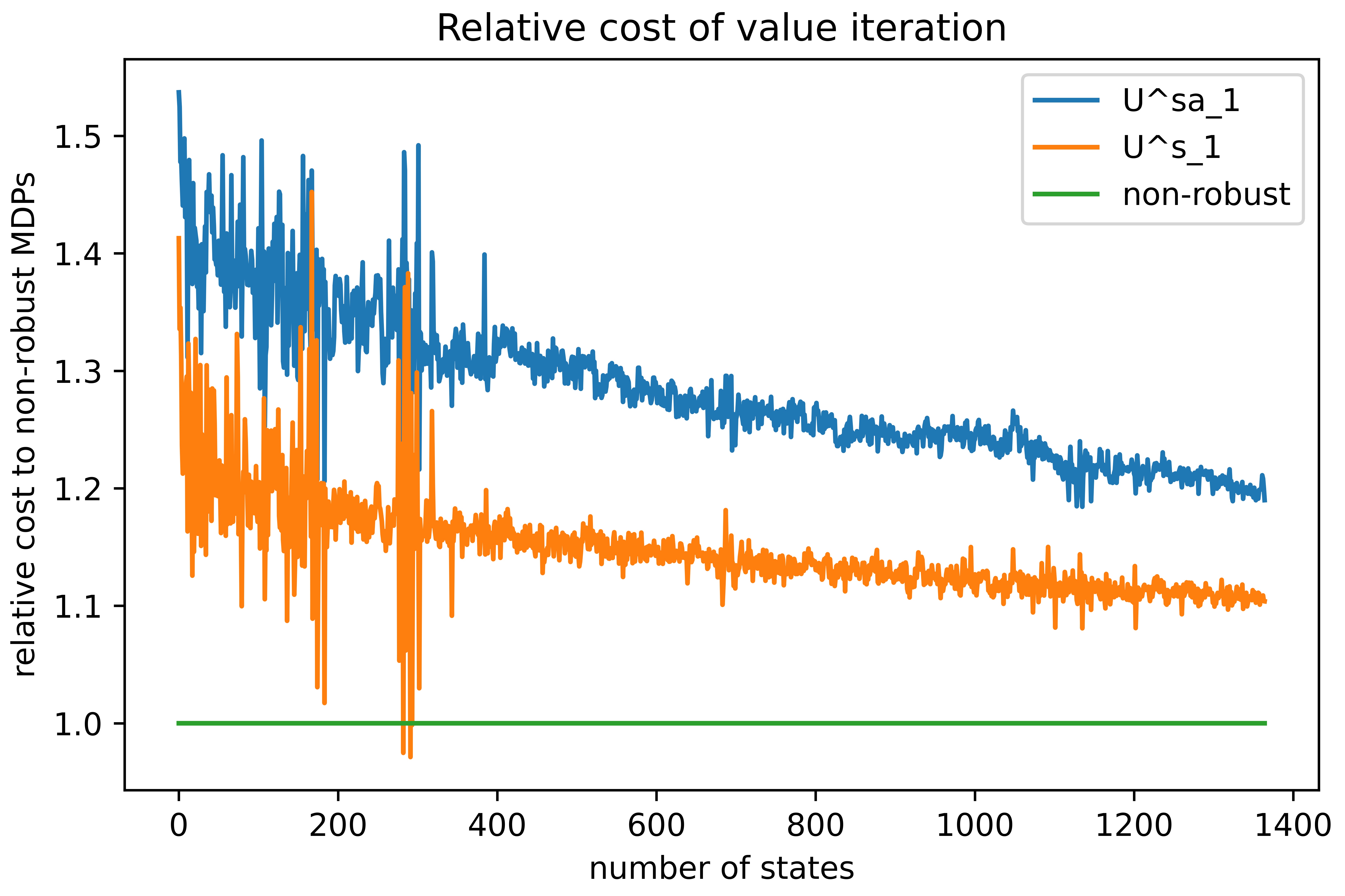
As our complexity analysis shows, value iterationโ€™s relative cost converges to 1 as the number of states increases while keeping the number of actions fixed. This is confirmed by Figure 1.

The rate of convergence for all the settings tested was the same as that of the non-robust setting, as predicted by the theory. The experiments ran a few times, resulting in some stochasticity in the results, but the trend is clear. Further details can be found in section G.

7 Conclusion and future work

We present an efficient robust value iteration for s-rectangular $L_{p}$-robust MDPs. Our method can be easily adapted to an online setting, as shown in Algorithm 2 for s-rectangular $L_{p}$-robust MDPs. Algorithm 2 is a two-time-scale algorithm, where the Q-values are approximated at a faster time scale and the value function is approximated from the Q-values at a slower time scale. The $p$-variance function $\kappa_{p}$ can be estimated in an online fashion using batches or other sophisticated methods. The convergence of the algorithm can be guaranteed from [8]; however, its analysis is left for future work.

Additionally, we introduce a novel value regularizer ($\kappa_{p}$) and a novel threshold policy which may help to obtain more robust and generalizable policies.

Further research could focus on other types of uncertainty sets, potentially resulting in different kinds of regularizers and optimal policies.

References

  • [1] Oren Anava and Kfir Levy. k*-nearest neighbors: From global to local. Advances in neural information processing systems, 29, 2016.
  • [2] Mahsa Asadi, Mohammadย Sadegh Talebi, Hippolyte Bourel, and Odalric-Ambrym Maillard. Model-based reinforcement learning exploiting state-action equivalence. CoRR, abs/1910.04077, 2019.
  • [3] Peter Auer, Thomas Jaksch, and Ronald Ortner. Near-optimal regret bounds for reinforcement learning. In D.ย Koller, D.ย Schuurmans, Y.ย Bengio, and L.ย Bottou, editors, Advances in Neural Information Processing Systems, volumeย 21. Curran Associates, Inc., 2008.
  • [4] Peter Auer and Ronald Ortner. Logarithmic online regret bounds for undiscounted reinforcement learning. In B.ย Schรถlkopf, J.ย Platt, and T.ย Hoffman, editors, Advances in Neural Information Processing Systems, volumeย 19. MIT Press, 2006.
  • [5] Mohammadย Gheshlaghi Azar, Ian Osband, and Rรฉmi Munos. Minimax regret bounds for reinforcement learning. In Doina Precup and Yeeย Whye Teh, editors, Proceedings of the 34th International Conference on Machine Learning, volumeย 70 of Proceedings of Machine Learning Research, pages 263โ€“272. PMLR, 06โ€“11 Aug 2017.
  • [6] J.ย Andrew Bagnell, Andrewย Y. Ng, and Jeffย G. Schneider. Solving uncertain markov decision processes. Technical report, Carnegie Mellon University, 2001.
  • [7] Bahram Behzadian, Marek Petrik, and Chinย Pang Ho. Fast algorithms for l_\infty-constrained s-rectangular robust mdps. In M.ย Ranzato, A.ย Beygelzimer, Y.ย Dauphin, P.S. Liang, and J.ย Wortman Vaughan, editors, Advances in Neural Information Processing Systems, volumeย 34, pages 25982โ€“25992. Curran Associates, Inc., 2021.
  • [8] Vivek Borkar. Stochastic Approximation: A Dynamical Systems Viewpoint. 01 2008.
  • [9] Esther Derman, Matthieu Geist, and Shie Mannor. Twice regularized mdps and the equivalence between robustness and regularization, 2021.
  • [10] Esther Derman and Shie Mannor. Distributional robustness and regularization in reinforcement learning, 2020.
  • [11] Benjamin Eysenbach and Sergey Levine. Maximum entropy rl (provably) solves some robust rl problems, 2021.
  • [12] Vineet Goyal and Julien Grand-Clรฉment. Robust markov decision process: Beyond rectangularity, 2018.
  • [13] Jean-Bastien Grill, Omar Darwicheย Domingues, Pierre Menard, Remi Munos, and Michal Valko. Planning in entropy-regularized markov decision processes and games. In H.ย Wallach, H.ย Larochelle, A.ย Beygelzimer, F.ย d'Alchรฉ-Buc, E.ย Fox, and R.ย Garnett, editors, Advances in Neural Information Processing Systems, volumeย 32. Curran Associates, Inc., 2019.
  • [14] Tuomas Haarnoja, Haoran Tang, Pieter Abbeel, and Sergey Levine. Reinforcement learning with deep energy-based policies, 2017.
  • [15] Graniย Adiwena Hanasusanto and Daniel Kuhn. Robust data-driven dynamic programming. In C.J. Burges, L.ย Bottou, M.ย Welling, Z.ย Ghahramani, and K.Q. Weinberger, editors, Advances in Neural Information Processing Systems, volumeย 26. Curran Associates, Inc., 2013.
  • [16] Chinย Pang Ho, Marek Petrik, and Wolfram Wiesemann. Partial policy iteration for l1-robust markov decision processes, 2020.
  • [17] Hisham Husain, Kamil Ciosek, and Ryota Tomioka. Regularized policies are reward robust, 2021.
  • [18] Garudย N. Iyengar. Robust dynamic programming. Mathematics of Operations Research, 30(2):257โ€“280, May 2005.
  • [19] Davidย L. Kaufman and Andrewย J. Schaefer. Robust modified policy iteration. INFORMS J. Comput., 25:396โ€“410, 2013.
  • [20] Xiang Li, Wenhao Yang, and Zhihua Zhang. A Regularized Approach to Sparse Optimal Policy in Reinforcement Learning. Curran Associates Inc., Red Hook, NY, USA, 2019.
  • [21] Tien Mai and Patrick Jaillet. Robust entropy-regularized markov decision processes, 2021.
  • [22] Shie Mannor, Ofir Mebel, and Huan Xu. Robust mdps with k-rectangular uncertainty. Math. Oper. Res., 41(4):1484โ€“1509, nov 2016.
  • [23] Shie Mannor, Duncan Simester, Peng Sun, and Johnย N. Tsitsiklis. Bias and variance in value function estimation. In Proceedings of the Twenty-First International Conference on Machine Learning, ICML โ€™04, pageย 72, New York, NY, USA, 2004. Association for Computing Machinery.
  • [24] Arnab Nilim and Laurentย El Ghaoui. Robust control of markov decision processes with uncertain transition matrices. Oper. Res., 53:780โ€“798, 2005.
  • [25] Charles Packer, Katelyn Gao, Jernej Kos, Philipp Krรคhenbรผhl, Vladlen Koltun, and Dawn Song. Assessing generalization in deep reinforcement learning, 2018.
  • [26] Martinย L. Puterman. Markov decision processes: Discrete stochastic dynamic programming. In Wiley Series in Probability and Statistics, 1994.
  • [27] John Schulman, Xiย Chen, and Pieter Abbeel. Equivalence between policy gradients and soft q-learning, 2017.
  • [28] Richardย S. Sutton and Andrewย G. Barto. Reinforcement Learning: An Introduction. The MIT Press, second edition, 2018.
  • [29] Aviv Tamar, Shie Mannor, and Huan Xu. Scaling up robust mdps using function approximation. In Ericย P. Xing and Tony Jebara, editors, Proceedings of the 31st International Conference on Machine Learning, volumeย 32 of Proceedings of Machine Learning Research, pages 181โ€“189, Bejing, China, 22โ€“24 Jun 2014. PMLR.
  • [30] Yue Wang and Shaofeng Zou. Online robust reinforcement learning with model uncertainty, 2021.
  • [31] Yue Wang and Shaofeng Zou. Policy gradient method for robust reinforcement learning, 2022.
  • [32] Wolfram Wiesemann, Daniel Kuhn, and Breรง Rustem. Robust markov decision processes. Mathematics of Operations Research, 38(1):153โ€“183, 2013.
  • [33] Huan Xu and Shie Mannor. Robustness and generalization, 2010.
  • [34] Chenyang Zhao, Olivier Sigaud, Freek Stulp, and Timothyย M. Hospedales. Investigating generalisation in continuous deep reinforcement learning, 2019.

How to read appendix

  1. 1.

    Section A contains related work.

  2. 2.

    Section B contains additional properties and results that couldnโ€™t be included in the main section for the sake of clarity and space. Many of the results in the main paper is special cases of the results in this section.

  3. 3.

    Section C contains the discussion on zero transition kernel (forbidden transitions).

  4. 4.

    Section D contains a possible connection this work to UCRL.

  5. 5.

    Section G contains additional experimental results and a detailed discussion.

  6. 6.

    All the proofs of the main body of the paper is presented in the section K and L.

  7. 7.

    Section I contains helper results for section K. Particularly, it discusses $p$-mean function $\omega_{p}$ and $p$-variance function $\kappa_{p}$.

  8. 8.

    Section J contains helper results for section K. Particularly, it discusses $L_{p}$ water pouring lemma, necessary to evaluate robust optimal Bellman operator (learning) for $\mathtt{s}$-rectangular $L_{p}$ robust MDPs.

  9. 9.

    Section L contains time complexity proof for model based algorithms.

  10. 10.

    Section E develops Q-learning machinery for $(\mathtt{sa})$-rectangular $L_{p}$ robust MDPs based on the results in the main section. It is not used in the main body or anywhere else, but this provides a good understanding for algorithms proposed in section F for $(\mathtt{sa})$-rectangular case.

  11. 11.

    Section F contains model-based algorithms for $\mathtt{s}$ and $(\mathtt{sa})$-rectangular $L_{p}$ robust MDPs. It also contains, remarks for special cases for $p=1,2,\infty$.

Appendix A Related Work

R-Contamination Uncertainty Robust MDPs

The paper [30] considers the following uncertainty set for some fixed constant $0\leq R\leq 1$,

$\displaystyle\mathcal{P}_{sa}=\{(1-R)(P_{0})(\cdot|s,a)+RP\mid P\in\Delta_{\mathcal{S}}\},\quad s\in\mathcal{S},a\in\mathcal{A},$ (9)

and $\mathcal{P}=\otimes_{s,a}\mathcal{P}_{s,a},\qquad\mathcal{U}=\{R_{0}\}\times\mathcal{P}$. The robust value function $v^{\pi}_{\mathcal{U}}$ is the fixed point of the robust Bellman operator defined as

(๐’ฏ๐’ฐฯ€โ€‹v)โ€‹(s):=assignsubscriptsuperscript๐’ฏ๐œ‹๐’ฐ๐‘ฃ๐‘ absent\displaystyle(\mathcal{T}^{\pi}_{\mathcal{U}}v)(s):= minPโˆˆ๐’ซโ€‹โˆ‘aฯ€โ€‹(a|s)โ€‹[R0โ€‹(s,a)+ฮณโ€‹โˆ‘sโ€ฒPโ€‹(sโ€ฒ|s,a)โ€‹vโ€‹(sโ€ฒ)],subscript๐‘ƒ๐’ซsubscript๐‘Ž๐œ‹conditional๐‘Ž๐‘ delimited-[]subscript๐‘…0๐‘ ๐‘Ž๐›พsubscriptsuperscript๐‘ โ€ฒ๐‘ƒconditionalsuperscript๐‘ โ€ฒ๐‘ ๐‘Ž๐‘ฃsuperscript๐‘ โ€ฒ\displaystyle\min_{P\in\mathcal{P}}\sum_{a}\pi(a|s)[R_{0}(s,a)+\gamma\sum_{s^{\prime}}P(s^{\prime}|s,a)v(s^{\prime})], (10)
$\displaystyle=$ โˆ‘aฯ€โ€‹(a|s)โ€‹[R0โ€‹(s,a)โˆ’ฮณโ€‹Rโ€‹maxsโกvโ€‹(s)+(1โˆ’R)โ€‹ฮณโ€‹โˆ‘sโ€ฒP0โ€‹(sโ€ฒ|s,a)โ€‹vโ€‹(sโ€ฒ)].subscript๐‘Ž๐œ‹conditional๐‘Ž๐‘ delimited-[]subscript๐‘…0๐‘ ๐‘Ž๐›พ๐‘…subscript๐‘ ๐‘ฃ๐‘ 1๐‘…๐›พsubscriptsuperscript๐‘ โ€ฒsubscript๐‘ƒ0conditionalsuperscript๐‘ โ€ฒ๐‘ ๐‘Ž๐‘ฃsuperscript๐‘ โ€ฒ\displaystyle\sum_{a}\pi(a|s)[R_{0}(s,a)-\gamma R\max_{s}v(s)+(1-R)\gamma\sum_{s^{\prime}}P_{0}(s^{\prime}|s,a)v(s^{\prime})]. (11)

And the optimal robust value function $v^{*}_{\mathcal{Ua}}$ is the fixed point of the optimal robust Bellman operator defined as

(๐’ฏ๐’ฐโˆ—โ€‹v)โ€‹(s):=assignsubscriptsuperscript๐’ฏ๐’ฐ๐‘ฃ๐‘ absent\displaystyle(\mathcal{T}^{*}_{\mathcal{U}}v)(s):= maxฯ€โกminPโˆˆ๐’ซโ€‹โˆ‘aฯ€โ€‹(a|s)โ€‹[R0โ€‹(s,a)+ฮณโ€‹(1โˆ’R)โ€‹โˆ‘sโ€ฒPโ€‹(sโ€ฒ|s,a)โ€‹vโ€‹(sโ€ฒ)],subscript๐œ‹subscript๐‘ƒ๐’ซsubscript๐‘Ž๐œ‹conditional๐‘Ž๐‘ delimited-[]subscript๐‘…0๐‘ ๐‘Ž๐›พ1๐‘…subscriptsuperscript๐‘ โ€ฒ๐‘ƒconditionalsuperscript๐‘ โ€ฒ๐‘ ๐‘Ž๐‘ฃsuperscript๐‘ โ€ฒ\displaystyle\max_{\pi}\min_{P\in\mathcal{P}}\sum_{a}\pi(a|s)[R_{0}(s,a)+\gamma(1-R)\sum_{s^{\prime}}P(s^{\prime}|s,a)v(s^{\prime})], (12)
$\displaystyle=$ maxaโก[R0โ€‹(s,a)โˆ’ฮณโ€‹Rโ€‹maxsโกvโ€‹(s)+ฮณโ€‹(1โˆ’R)โ€‹โˆ‘sโ€ฒP0โ€‹(sโ€ฒ|s,a)โ€‹vโ€‹(sโ€ฒ)].subscript๐‘Žsubscript๐‘…0๐‘ ๐‘Ž๐›พ๐‘…subscript๐‘ ๐‘ฃ๐‘ ๐›พ1๐‘…subscriptsuperscript๐‘ โ€ฒsubscript๐‘ƒ0conditionalsuperscript๐‘ โ€ฒ๐‘ ๐‘Ž๐‘ฃsuperscript๐‘ โ€ฒ\displaystyle\max_{a}[R_{0}(s,a)-\gamma R\max_{s}v(s)+\gamma(1-R)\sum_{s^{\prime}}P_{0}(s^{\prime}|s,a)v(s^{\prime})]. (13)

Since, the uncertainty set is sa-rectangular, hence the map is a contraction [24], so the robust value iteration here, will also converge linearly similar to non-robust MDPs. It is also possible to obtain Q-learning as following

Qn+1โ€‹(s,a)=R0โ€‹(s,a)โˆ’ฮณโ€‹Rโ€‹maxs,aโกQnโ€‹(s,a)+ฮณโ€‹(1โˆ’R)โ€‹โˆ‘sโ€ฒP0โ€‹(sโ€ฒ|s,a)โ€‹maxsโ€ฒโกQnโ€‹(sโ€ฒ,aโ€ฒ).subscript๐‘„๐‘›1๐‘ ๐‘Žsubscript๐‘…0๐‘ ๐‘Ž๐›พ๐‘…subscript๐‘ ๐‘Žsubscript๐‘„๐‘›๐‘ ๐‘Ž๐›พ1๐‘…subscriptsuperscript๐‘ โ€ฒsubscript๐‘ƒ0conditionalsuperscript๐‘ โ€ฒ๐‘ ๐‘Žsubscriptsuperscript๐‘ โ€ฒsubscript๐‘„๐‘›superscript๐‘ โ€ฒsuperscript๐‘Žโ€ฒ\displaystyle Q_{n+1}(s,a)=R_{0}(s,a)-\gamma R\max_{s,a}Q_{n}(s,a)+\gamma(1-R)\sum_{s^{\prime}}P_{0}(s^{\prime}|s,a)\max_{s^{\prime}}Q_{n}(s^{\prime},a^{\prime}). (14)

Convergence of the above Q-learning follows from the contraction of robust value iteration. Further, it is easy to see that model-free Q-learning can be obtained from the above.

A follow-up work [31] proposes a policy gradient method for the same.

Proposition 1.

(Theorem 3.3 of [31]) Consider a class of policies ฮ ฮ \Pi satisfying Assumption 3.2 of [31]. The gradient of the robust return is given by

$\displaystyle\nabla\rho^{\pi_{\theta}}=$ ฮณโ€‹R(1โˆ’ฮณ)โ€‹(1โˆ’ฮณ+ฮณโ€‹R)โ€‹โˆ‘s,adฮผฯ€ฮธโ€‹(s,a)โ€‹โˆ‡ฯ€ฮธโ€‹(a|s)โ€‹Q๐’ฐฯ€ฮธโ€‹(s,a)๐›พ๐‘…1๐›พ1๐›พ๐›พ๐‘…subscript๐‘ ๐‘Žsubscriptsuperscript๐‘‘subscript๐œ‹๐œƒ๐œ‡๐‘ ๐‘Žโˆ‡subscript๐œ‹๐œƒconditional๐‘Ž๐‘ subscriptsuperscript๐‘„subscript๐œ‹๐œƒ๐’ฐ๐‘ ๐‘Ž\displaystyle\frac{\gamma R}{(1-\gamma)(1-\gamma+\gamma R)}\sum_{s,a}d^{\pi_{\theta}}_{\mu}(s,a)\nabla{\pi_{\theta}}(a|s)Q^{\pi_{\theta}}_{\mathcal{U}}(s,a)
+11โˆ’ฮณ+ฮณโ€‹Rโ€‹โˆ‘s,adsฮธฯ€ฮธโ€‹(s,a)โ€‹โˆ‡ฯ€ฮธโ€‹(a|s)โ€‹Q๐’ฐฯ€ฮธโ€‹(s,a),11๐›พ๐›พ๐‘…subscript๐‘ ๐‘Žsubscriptsuperscript๐‘‘subscript๐œ‹๐œƒsubscript๐‘ ๐œƒ๐‘ ๐‘Žโˆ‡subscript๐œ‹๐œƒconditional๐‘Ž๐‘ subscriptsuperscript๐‘„subscript๐œ‹๐œƒ๐’ฐ๐‘ ๐‘Ž\displaystyle\qquad+\frac{1}{1-\gamma+\gamma R}\sum_{s,a}d^{\pi_{\theta}}_{s_{\theta}}(s,a)\nabla{\pi_{\theta}}(a|s)Q^{\pi_{\theta}}_{\mathcal{U}}(s,a),

where sฮธโˆˆargโ€‹maxโกv๐’ฐฯ€ฮธโ€‹(s)subscript๐‘ ๐œƒargsubscriptsuperscript๐‘ฃsubscript๐œ‹๐œƒ๐’ฐ๐‘ s_{\theta}\in\text{arg}\max v^{\pi_{\theta}}_{\mathcal{U}}(s), and $Q^{\pi}_{\mathcal{U}}(s,a)=\sum_{a}\pi(a|s)\bigm{[}R_{0}(s,a)-\gamma R\max_{s}v^{\pi}_{\mathcal{U}}(s)+\gamma(1-R)\sum_{s^{\prime}}P_{0}(s^{\prime}|s,a)v^{\pi}_{\mathcal{U}}(s^{\prime})\bigm{]}.$

The work shows that the proposed robust policy gradient method converges to the global optimum asymptotically under direct policy parameterization.

The uncertainty set considered here, is sa-rectangular, as uncertainty in each state-action is independent, hence the regularizer term (ฮณโ€‹Rโ€‹maxsโกvโ€‹(s))๐›พ๐‘…subscript๐‘ ๐‘ฃ๐‘ (\gamma R\max_{s}v(s)) is independent of policy, and the optimal (and greedy) policy is deterministic. It is unclear, how the uncertainty set can be generalized to the s๐‘ s-rectangular case. Observe that the above results resemble very closely our sa-rectangular $L_{1}$ robust MDPs results.

Twice Regularized MDPs

The paper [9] converts robust MDPs to twice regularized MDPs, and proposes a gradient based policy iteration method for solving them.

Proposition 2.

(corollary 3.1 of [9]) (s-rectangular reward robust policy evaluation) Let the uncertainty set be $\mathcal{U}=(R_{0}+\mathcal{R})\times\{P_{0}\}$, where โ„›s={rsโˆˆ๐‘๐’œโˆฃโˆฅrsโˆฅโ‰คฮฑs}subscriptโ„›๐‘ conditional-setsubscript๐‘Ÿ๐‘ superscript๐‘๐’œdelimited-โˆฅโˆฅsubscript๐‘Ÿ๐‘ subscript๐›ผ๐‘ \mathcal{R}_{s}=\{r_{s}\in\mathbf{R}^{\mathcal{A}}\mid\lVert r_{s}\rVert\leq\alpha_{s}\} for all sโˆˆ๐’ฎ๐‘ ๐’ฎs\in\mathcal{S}. Then the robust value function $v^{\pi}_{\mathcal{U}}$ is the optimal solution to the convex optimization problem:

$$\max_{v\in\mathbf{R}^{\mathcal{A}}}\langle\mu,v\rangle\quad s.t.\quad v(s)\leq(\mathcal{T}^{\pi}_{R_{0},P_{0}}v)(s)-\alpha_{s}\lVert\pi_{s}\rVert,\qquad\forall s\in\mathcal{S}.$$

It derives the policy gradient for reward robust MDPs to obtain the optimal robust policy $\pi^{*}_{\mathcal{U}}$.

Proposition 3.

(Proposition 3.2 of [9]) (s-rectangular reward robust policy gradient) Let the uncertainty set be $\mathcal{U}=(R_{0}+\mathcal{R})\times\{P_{0}\}$, where โ„›s={rsโˆˆ๐‘๐’œโˆฃโˆฅrsโˆฅโ‰คฮฑs}subscriptโ„›๐‘ conditional-setsubscript๐‘Ÿ๐‘ superscript๐‘๐’œdelimited-โˆฅโˆฅsubscript๐‘Ÿ๐‘ subscript๐›ผ๐‘ \mathcal{R}_{s}=\{r_{s}\in\mathbf{R}^{\mathcal{A}}\mid\lVert r_{s}\rVert\leq\alpha_{s}\} for all sโˆˆ๐’ฎ๐‘ ๐’ฎs\in\mathcal{S}. Then the gradient of the reward robust objective $\rho^{\pi}_{\mathcal{U}}:=\langle\mu,v^{\pi}_{\mathcal{U}}\rangle$ is given by

$$\nabla\rho^{\pi}_{\mathcal{U}}=\mathbf{E}_{(s,a)\sim d^{\pi}_{P_{0}}}\Bigm{[}\nabla\ln(\pi(a|s))\bigm{(}Q^{\pi}_{\mathcal{U}}(s,a)-\alpha_{s}\frac{\pi(a|s)}{\lVert\pi_{s}\rVert}\bigm{)}\Bigm{]},$$

where Q๐’ฐฯ€โ€‹(s,a):=min(R,P)โˆˆ๐’ฐโก[Rโ€‹(s,a)+ฮณโ€‹โˆ‘sโ€ฒPโ€‹(sโ€ฒ|s,a)โ€‹v๐’ฐฯ€โ€‹(sโ€ฒ)].assignsubscriptsuperscript๐‘„๐œ‹๐’ฐ๐‘ ๐‘Žsubscript๐‘…๐‘ƒ๐’ฐ๐‘…๐‘ ๐‘Ž๐›พsubscriptsuperscript๐‘ โ€ฒ๐‘ƒconditionalsuperscript๐‘ โ€ฒ๐‘ ๐‘Žsubscriptsuperscript๐‘ฃ๐œ‹๐’ฐsuperscript๐‘ โ€ฒQ^{\pi}_{\mathcal{U}}(s,a):=\min_{(R,P)\in\mathcal{U}}[R(s,a)+\gamma\sum_{s^{\prime}}P(s^{\prime}|s,a)v^{\pi}_{\mathcal{U}}(s^{\prime})].

Proposition 4.

(Corollary 4.1 of [9]) (s-rectangular general robust policy evaluation) Let the uncertainty set be $\mathcal{U}=(R_{0}+\mathcal{R})\times\{P_{0}+\mathcal{P}\}$, where โ„›s={rsโˆˆ๐‘๐’œโˆฃโˆฅrsโˆฅโ‰คฮฑs}subscriptโ„›๐‘ conditional-setsubscript๐‘Ÿ๐‘ superscript๐‘๐’œdelimited-โˆฅโˆฅsubscript๐‘Ÿ๐‘ subscript๐›ผ๐‘ \mathcal{R}_{s}=\{r_{s}\in\mathbf{R}^{\mathcal{A}}\mid\lVert r_{s}\rVert\leq\alpha_{s}\} and ๐’ซs={Psโˆˆ๐‘๐’ฎร—๐’œโˆฃโˆฅPsโˆฅโ‰คฮฒs}subscript๐’ซ๐‘ conditional-setsubscript๐‘ƒ๐‘ superscript๐‘๐’ฎ๐’œdelimited-โˆฅโˆฅsubscript๐‘ƒ๐‘ subscript๐›ฝ๐‘ \mathcal{P}_{s}=\{P_{s}\in\mathbf{R}^{\mathcal{S}\times\mathcal{A}}\mid\lVert P_{s}\rVert\leq\beta_{s}\} for all sโˆˆ๐’ฎ๐‘ ๐’ฎs\in\mathcal{S}. Then the robust value function $v^{\pi}_{\mathcal{U}}$ is the optimal solution to the convex optimization problem:

$$\max_{v\in\mathbf{R}^{\mathcal{A}}}\langle\mu,v\rangle\quad s.t.\quad v(s)\leq(\mathcal{T}^{\pi}_{R_{0},P_{0}}v)(s)-\alpha_{s}\lVert\pi_{s}\rVert-\gamma\beta_{s}\lVert v\rVert\lVert\pi_{s}\rVert,\qquad\forall s\in\mathcal{S}.$$

Same as the reward robust case, the paper tries to find a policy gradient method to obtain the optimal robust policy. Unfortunately, the dependence of regularizer terms on value makes it a very difficult task. Hence it proposes the $R^{2}$MPI algorithm (algorithm 1 of ย [9]) for the purpose that optimizing the greedy step via projection onto the simplex using a black box solver. Note that the above proposition is not same as our policy evaluation (although it looks similar), it requires some extra assumptions (assumption 5.1 ย [9]) and lot of work ensure $R^{2}$ Bellman operator is contraction etc. In our case, we directly evaluate robust Bellman operator that has already proven to be a contraction, hence we donโ€™t require any extra assumption nor any other work as ย [9].

Our work makes improvements over this work by explicitly solving both policy evaluation and policy improvement in general robust MDPs. It also makes more realistic assumptions on the transition kernel uncertainty set.

Regularizer solves Robust MDPs

The work [11] looks in the opposite direction than we do. It investigates the impact of the popularly used entropy regularizer on robustness. It finds that MaxEnt can be used to maximize a lower bound on a certain robust RL objective (reward robust).

As we noticed that โˆฅฯ€sโˆฅqsubscriptdelimited-โˆฅโˆฅsubscript๐œ‹๐‘ ๐‘ž\lVert\pi_{s}\rVert_{q} behaves like entropy in our regularization. Further, our work also deals with uncertainty in transition kernel in addition to the uncertainty in reward function.

Upper Confidence RL

The upper confidence setting in [4, 3] is very similar to our $L_{p}$ robust setting. We refer to this discussion in section D.

Appendix B S-rectangular: More Properties

Definition 1.

We begin with the following notational definitions.

  1. 1.

    $Q$-value at value function $v$ is defined as

    Qvโ€‹(s,a):=R0โ€‹(s,a)+ฮณโ€‹โˆ‘sโ€ฒP0โ€‹(sโ€ฒ|s,a)โ€‹vโ€‹(sโ€ฒ).assignsuperscript๐‘„๐‘ฃ๐‘ ๐‘Žsubscript๐‘…0๐‘ ๐‘Ž๐›พsubscriptsuperscript๐‘ โ€ฒsubscript๐‘ƒ0conditionalsuperscript๐‘ โ€ฒ๐‘ ๐‘Ž๐‘ฃsuperscript๐‘ โ€ฒQ^{v}(s,a):=R_{0}(s,a)+\gamma\sum_{s^{\prime}}P_{0}(s^{\prime}|s,a)v(s^{\prime}).
  2. 2.

    Optimal $Q$-value is defined as

    Q๐’ฐโˆ—โ€‹(s,a)=R0โ€‹(s,a)+ฮณโ€‹โˆ‘sโ€ฒP0โ€‹(sโ€ฒ|s,a)โ€‹v๐’ฐโˆ—โ€‹(sโ€ฒ)subscriptsuperscript๐‘„๐’ฐ๐‘ ๐‘Žsubscript๐‘…0๐‘ ๐‘Ž๐›พsubscriptsuperscript๐‘ โ€ฒsubscript๐‘ƒ0conditionalsuperscript๐‘ โ€ฒ๐‘ ๐‘Žsubscriptsuperscript๐‘ฃ๐’ฐsuperscript๐‘ โ€ฒQ^{*}_{\mathcal{U}}(s,a)=R_{0}(s,a)+\gamma\sum_{s^{\prime}}P_{0}(s^{\prime}|s,a)v^{*}_{\mathcal{U}}(s^{\prime})
  3. 3.

    With little abuse of notation, Qโ€‹(s,ai)๐‘„๐‘ subscript๐‘Ž๐‘–Q(s,a_{i}) shall denote the $i$th best value in state s๐‘ s, that is

    $$Q(s,a_{1})\geq Q(s,a_{2})\geq,\cdots,\geq Q(s,a_{A}).$$
  4. 4.

    $\pi^{v}_{\mathcal{U}}$ denotes the greedy policy at value function $v$, that is

    $$\mathcal{T}^{*}_{\mathcal{U}}v=\mathcal{T}^{\pi^{v}_{\mathcal{U}}}_{\mathcal{U}}v.$$
  5. 5.

    ฯ‡pโ€‹(s)subscript๐œ’๐‘๐‘ \chi_{p}(s) denotes the number of active actions in state s๐‘ s in s-rectangular $L_{p}$ robust MDPs, defined as

    $$\chi_{p}(s):=\bigm{\lvert}\{a\mid\pi^{*}_{\mathcal{U}^{s}_{p}}(a|s)\geq 0\}\bigm{\rvert}.$$
  6. 6.

    ฯ‡pโ€‹(p,s)subscript๐œ’๐‘๐‘๐‘ \chi_{p}(p,s) denotes the number of active actions in state s๐‘ s at value function $v$ in s-rectangular $L_{p}$ robust MDPs, defined as

    $$\chi_{p}(v,s):=\bigm{\lvert}\{a\mid\pi^{v}_{\mathcal{U}^{s}_{p}}(a|s)\geq 0\}\bigm{\rvert}.$$

We saw above that optimal policy in s-rectangular robust MDPs may be stochastic. The action that has a positive advantage is active and the rest are inactive. Let ฯ‡pโ€‹(s)subscript๐œ’๐‘๐‘ \chi_{p}(s) be the number of active actions in state s๐‘ s, defined as

$\displaystyle\chi_{p}(s):=\bigm{\lvert}\{a\mid\pi^{*}_{\mathcal{U}^{s}_{p}}(a|s)\geq 0\}\bigm{\rvert}=\bigm{\lvert}\{a\mid Q^{*}_{\mathcal{U}^{s}_{p}}(s,a)\geq v^{*}_{\mathcal{U}^{s}_{p}}(s)\}\bigm{\rvert}.$ (15)

Last equality comes from Theorem 4. One direct relation between Q-value and value function is given by

$\displaystyle v^{*}_{\mathcal{U}^{s}_{p}}(s)=\sum_{a}\pi^{*}_{\mathcal{U}^{s}_{p}}(a|s)\Bigm{[}-\bigm{(}\alpha_{s}+\gamma\beta_{s}\kappa_{q}(v)\bigm{)}\lVert\pi^{*}_{\mathcal{U}^{s}_{p}}(\cdot|s)\rVert_{q}+Q^{*}_{\mathcal{U}^{s}_{p}}(s,a)\Bigm{]}.$ (16)

The above relation is very convoluted compared to non-robust and sa-rectangular robust cases. The property below illuminates an interesting relation.

Property 1.

(Optimal Value vs Q-value) v๐’ฐpsโˆ—โ€‹(s)subscriptsuperscript๐‘ฃsubscriptsuperscript๐’ฐ๐‘ ๐‘๐‘ v^{*}_{\mathcal{U}^{s}_{p}}(s) is bounded by the Q-value of ฯ‡pโ€‹(s)subscript๐œ’๐‘๐‘ \chi_{p}(s)th and (ฯ‡pโ€‹(s)+1)subscript๐œ’๐‘๐‘ 1(\chi_{p}(s)+1)th actions, that is ,

Q๐’ฐpsโˆ—โ€‹(s,aฯ‡pโ€‹(s)+1)<v๐’ฐpsโˆ—โ€‹(s)โ‰คQ๐’ฐpsโˆ—โ€‹(s,aฯ‡pโ€‹(s)).subscriptsuperscript๐‘„subscriptsuperscript๐’ฐ๐‘ ๐‘๐‘ subscript๐‘Žsubscript๐œ’๐‘๐‘ 1subscriptsuperscript๐‘ฃsubscriptsuperscript๐’ฐ๐‘ ๐‘๐‘ subscriptsuperscript๐‘„subscriptsuperscript๐’ฐ๐‘ ๐‘๐‘ subscript๐‘Žsubscript๐œ’๐‘๐‘ Q^{*}_{\mathcal{U}^{s}_{p}}(s,a_{\chi_{p}(s)+1})<v^{*}_{\mathcal{U}^{s}_{p}}(s)\leq Q^{*}_{\mathcal{U}^{s}_{p}}(s,a_{\chi_{p}(s)}).

This special case of the property 2, similarly table 6 is special case of table 8.

Table 6: Optimal value function and Q-value
vโˆ—โ€‹(s)=maxaโกQโˆ—โ€‹(s,a)superscript๐‘ฃ๐‘ subscript๐‘Žsuperscript๐‘„๐‘ ๐‘Žv^{*}(s)=\max_{a}Q^{*}(s,a) Best value
v๐’ฐpsโ€‹aโˆ—โ€‹(s)=maxaโก[ฮฑs,aโˆ’ฮณโ€‹ฮฒs,aโ€‹ฮบqโ€‹(v๐’ฐpsโ€‹aโˆ—)โˆ’Q๐’ฐpsโ€‹aโˆ—โ€‹(s,a)]subscriptsuperscript๐‘ฃsubscriptsuperscript๐’ฐ๐‘ ๐‘Ž๐‘๐‘ subscript๐‘Žsubscript๐›ผ๐‘ ๐‘Ž๐›พsubscript๐›ฝ๐‘ ๐‘Žsubscript๐œ…๐‘žsubscriptsuperscript๐‘ฃsubscriptsuperscript๐’ฐ๐‘ ๐‘Ž๐‘subscriptsuperscript๐‘„subscriptsuperscript๐’ฐ๐‘ ๐‘Ž๐‘๐‘ ๐‘Žv^{*}_{\mathcal{U}^{sa}_{p}}(s)=\max_{a}[\alpha_{s,a}-\gamma\beta_{s,a}\kappa_{q}(v^{*}_{\mathcal{U}^{sa}_{p}})-Q^{*}_{\mathcal{U}^{sa}_{p}}(s,a)] Best regularized value
Q๐’ฐpsโˆ—โ€‹(s,aฯ‡pโ€‹(s)+1)<v๐’ฐpsโˆ—โ€‹(s)โ‰คQ๐’ฐpsโˆ—โ€‹(s,aฯ‡pโ€‹(s))subscriptsuperscript๐‘„subscriptsuperscript๐’ฐ๐‘ ๐‘๐‘ subscript๐‘Žsubscript๐œ’๐‘๐‘ 1subscriptsuperscript๐‘ฃsubscriptsuperscript๐’ฐ๐‘ ๐‘๐‘ subscriptsuperscript๐‘„subscriptsuperscript๐’ฐ๐‘ ๐‘๐‘ subscript๐‘Žsubscript๐œ’๐‘๐‘ Q^{*}_{\mathcal{U}^{s}_{p}}(s,a_{\chi_{p}(s)+1})<v^{*}_{\mathcal{U}^{s}_{p}}(s)\leq Q^{*}_{\mathcal{U}^{s}_{p}}(s,a_{\chi_{p}(s)}) Sandwich!
where $v^{*},Q^{*}$ is the optimal value function and Q-value respectively
of non-robust MDP.

The same is true for the non-optimal Q-value and value function.

Theorem 5.

(Greedy policy) The greedy policy ฯ€๐’ฐpsvsubscriptsuperscript๐œ‹๐‘ฃsubscriptsuperscript๐’ฐ๐‘ ๐‘\pi^{v}_{\mathcal{U}^{s}_{p}} is a threshold policy, that is proportional to the advantage function, that is

$$\pi^{v}_{\mathcal{U}^{s}_{p}}(a|s)\propto\bigm{(}Q^{v}(s,a)-(\mathcal{T}^{*}_{\mathcal{U}^{s}_{p}}v)(s)\bigm{)}^{p-1}\mathbf{1}\bigm{(}Q^{v}(s,a)\geq(\mathcal{T}^{*}_{\mathcal{U}^{s}_{p}}v)(s)\bigm{)}.$$

The above theorem is proved in the appendix, and Theorem 4 is its special case. So is table 3 special case of table 7.

Table 7: Greedy policy at value function $v$
$\mathcal{U}$ ฯ€๐’ฐvโ€‹(a|s)โˆproportional-tosubscriptsuperscript๐œ‹๐‘ฃ๐’ฐconditional๐‘Ž๐‘ absent\pi^{v}_{\mathcal{U}}(a|s)\propto remark
๐’ฐpssubscriptsuperscript๐’ฐ๐‘ ๐‘\mathcal{U}^{s}_{p} (Qvโ€‹(s,a)โˆ’(๐’ฏ๐’ฐโˆ—โ€‹v)โ€‹(s))pโˆ’1โ€‹๐Ÿโ€‹(A๐’ฐvโ€‹(s,a)โ‰ฅ0)superscriptsuperscript๐‘„๐‘ฃ๐‘ ๐‘Žsubscriptsuperscript๐’ฏ๐’ฐ๐‘ฃ๐‘ ๐‘11subscriptsuperscript๐ด๐‘ฃ๐’ฐ๐‘ ๐‘Ž0(Q^{v}(s,a)-(\mathcal{T}^{*}_{\mathcal{U}}v)(s))^{p-1}\mathbf{1}(A^{v}_{\mathcal{U}}(s,a)\geq 0) top actions proportional to
$(p-1)$th power of its advantage
๐’ฐ1ssubscriptsuperscript๐’ฐ๐‘ 1\mathcal{U}^{s}_{1} ๐Ÿโ€‹(A๐’ฐvโ€‹(s,a)โ‰ฅ0)โˆ‘a๐Ÿโ€‹(A๐’ฐvโ€‹(s,a)โ‰ฅ0)1subscriptsuperscript๐ด๐‘ฃ๐’ฐ๐‘ ๐‘Ž0subscript๐‘Ž1subscriptsuperscript๐ด๐‘ฃ๐’ฐ๐‘ ๐‘Ž0\frac{\mathbf{1}(A^{v}_{\mathcal{U}}(s,a)\geq 0)}{\sum_{a}\mathbf{1}(A^{v}_{\mathcal{U}}(s,a)\geq 0)} top actions with uniform probability
๐’ฐ2ssubscriptsuperscript๐’ฐ๐‘ 2\mathcal{U}^{s}_{2} $\frac{A^{v}_{\mathcal{U}}(s,a)\mathbf{1}A^{v}_{\mathcal{U}}(s,a)\geq 0)}{\sum_{a}A^{v}_{\mathcal{U}}(s,a)\mathbf{1}(A^{v}_{\mathcal{U}}(s,a)\geq 0)}$ top actions proportion to advantage
๐’ฐโˆžssubscriptsuperscript๐’ฐ๐‘ \mathcal{U}^{s}_{\infty} argโ€‹maxaโˆˆ๐’œโกQvโ€‹(s,a)argsubscript๐‘Ž๐’œsuperscript๐‘„๐‘ฃ๐‘ ๐‘Ž\text{arg}\max_{a\in\mathcal{A}}Q^{v}(s,a) best action
$\mathcal{U}^{\mathtt{sa}}_{p}$ argโ€‹maxaโก[โˆ’ฮฑsโ€‹aโˆ’ฮณโ€‹ฮฒsโ€‹aโ€‹ฮบqโ€‹(v)+Qvโ€‹(s,a)]argsubscript๐‘Žsubscript๐›ผ๐‘ ๐‘Ž๐›พsubscript๐›ฝ๐‘ ๐‘Žsubscript๐œ…๐‘ž๐‘ฃsuperscript๐‘„๐‘ฃ๐‘ ๐‘Ž\text{arg}\max_{a}[-\alpha_{sa}-\gamma\beta_{sa}\kappa_{q}(v)+Q^{v}(s,a)] best action
where A๐’ฐvโ€‹(s,a)=Qvโ€‹(s,a)โˆ’(๐’ฏ๐’ฐโˆ—โ€‹v)โ€‹(s)subscriptsuperscript๐ด๐‘ฃ๐’ฐ๐‘ ๐‘Žsuperscript๐‘„๐‘ฃ๐‘ ๐‘Žsubscriptsuperscript๐’ฏ๐’ฐ๐‘ฃ๐‘ A^{v}_{\mathcal{U}}(s,a)=Q^{v}(s,a)-(\mathcal{T}^{*}_{\mathcal{U}}v)(s) and Qvโ€‹(s,a)=R0โ€‹(s,a)+ฮณโ€‹โˆ‘sโ€ฒP0โ€‹(sโ€ฒ|s,a)โ€‹vโ€‹(sโ€ฒ)superscript๐‘„๐‘ฃ๐‘ ๐‘Žsubscript๐‘…0๐‘ ๐‘Ž๐›พsubscriptsuperscript๐‘ โ€ฒsubscript๐‘ƒ0conditionalsuperscript๐‘ โ€ฒ๐‘ ๐‘Ž๐‘ฃsuperscript๐‘ โ€ฒQ^{v}(s,a)=R_{0}(s,a)+\gamma\sum_{s^{\prime}}P_{0}(s^{\prime}|s,a)v(s^{\prime}).

The above result states that the greedy policy takes actions that have a positive advantage, so we have.

$\displaystyle\chi_{p}(v,s):=\bigm{\lvert}\{a\mid\pi^{v}_{\mathcal{U}^{s}_{p}}(a|s)\geq 0\}\bigm{\rvert}=\bigm{\lvert}\{a\mid Q^{v}(s,a)\geq(\mathcal{T}^{*}_{\mathcal{U}^{s}_{p}})v(s)\}\bigm{\rvert}.$ (17)
Property 2.

(Greedy Value vs Q-value) (๐’ฏ๐’ฐpsโˆ—โ€‹v)โ€‹(s)subscriptsuperscript๐’ฏsubscriptsuperscript๐’ฐ๐‘ ๐‘๐‘ฃ๐‘ (\mathcal{T}^{*}_{\mathcal{U}^{s}_{p}}v)(s) is bounded by the Q-value of ฯ‡pโ€‹(v,s)subscript๐œ’๐‘๐‘ฃ๐‘ \chi_{p}(v,s)th and (ฯ‡pโ€‹(v,s)+1)subscript๐œ’๐‘๐‘ฃ๐‘ 1(\chi_{p}(v,s)+1)th actions, that is ,

Qvโ€‹(s,aฯ‡pโ€‹(v,s)+1)<(๐’ฏ๐’ฐpsโˆ—โ€‹v)โ€‹(s)โ‰คQvโ€‹(s,aฯ‡pโ€‹(v,s)).superscript๐‘„๐‘ฃ๐‘ subscript๐‘Žsubscript๐œ’๐‘๐‘ฃ๐‘ 1subscriptsuperscript๐’ฏsubscriptsuperscript๐’ฐ๐‘ ๐‘๐‘ฃ๐‘ superscript๐‘„๐‘ฃ๐‘ subscript๐‘Žsubscript๐œ’๐‘๐‘ฃ๐‘ Q^{v}(s,a_{\chi_{p}(v,s)+1})<(\mathcal{T}^{*}_{\mathcal{U}^{s}_{p}}v)(s)\leq Q^{v}(s,a_{\chi_{p}(v,s)}).
Table 8: Greedy value function and Q-value
(๐’ฏโˆ—โ€‹v)โ€‹(s)=maxaโกQvโ€‹(s,a)superscript๐’ฏ๐‘ฃ๐‘ subscript๐‘Žsuperscript๐‘„๐‘ฃ๐‘ ๐‘Ž(\mathcal{T}^{*}v)(s)=\max_{a}Q^{v}(s,a) Best value
(๐’ฏ๐’ฐpsโ€‹aโˆ—)โ€‹vโ€‹(s)=maxaโก[ฮฑs,aโˆ’ฮณโ€‹ฮฒs,aโ€‹ฮบqโ€‹(v)โˆ’Qvโ€‹(s,a)]subscriptsuperscript๐’ฏsubscriptsuperscript๐’ฐ๐‘ ๐‘Ž๐‘๐‘ฃ๐‘ subscript๐‘Žsubscript๐›ผ๐‘ ๐‘Ž๐›พsubscript๐›ฝ๐‘ ๐‘Žsubscript๐œ…๐‘ž๐‘ฃsuperscript๐‘„๐‘ฃ๐‘ ๐‘Ž(\mathcal{T}^{*}_{\mathcal{U}^{sa}_{p}})v(s)=\max_{a}[\alpha_{s,a}-\gamma\beta_{s,a}\kappa_{q}(v)-Q^{v}(s,a)] Best regularized value
Qvโ€‹(s,aฯ‡pโ€‹(v,s)+1)<(๐’ฏ๐’ฐpsโˆ—)โ€‹vโ€‹(s)โ‰คQvโ€‹(s,aฯ‡pโ€‹(v,s))superscript๐‘„๐‘ฃ๐‘ subscript๐‘Žsubscript๐œ’๐‘๐‘ฃ๐‘ 1subscriptsuperscript๐’ฏsubscriptsuperscript๐’ฐ๐‘ ๐‘๐‘ฃ๐‘ superscript๐‘„๐‘ฃ๐‘ subscript๐‘Žsubscript๐œ’๐‘๐‘ฃ๐‘ Q^{v}(s,a_{\chi_{p}(v,s)+1})<(\mathcal{T}^{*}_{\mathcal{U}^{s}_{p}})v(s)\leq Q^{v}(s,a_{\chi_{p}(v,s)}) Sandwich!
where $Q^{v}(s,a_{1})\geq,\cdots,\geq Q^{v}(s,a_{A}).$

The property below states that we can compute the number of active actions ฯ‡pโ€‹(v,s)subscript๐œ’๐‘๐‘ฃ๐‘ \chi_{p}(v,s) (and ฯ‡pโ€‹(s)subscript๐œ’๐‘๐‘ \chi_{p}(s)) directly without computing greedy (optimal) policy.

Property 3.

ฯ‡pโ€‹(v,s)subscript๐œ’๐‘๐‘ฃ๐‘ \chi_{p}(v,s) is number of actions that has positive advantage, that is

$$\chi_{p}(v,s):=\max\{k\mid\sum_{i=1}^{k}\bigm{(}Q^{v}(s,a_{i})-Q^{v}(s,a_{k})\bigm{)}^{p}\leq\sigma^{p}\},$$

where ฯƒ=ฮฑs+ฮณโ€‹ฮฒsโ€‹ฮบqโ€‹(v)๐œŽsubscript๐›ผ๐‘ ๐›พsubscript๐›ฝ๐‘ subscript๐œ…๐‘ž๐‘ฃ\sigma=\alpha_{s}+\gamma\beta_{s}\kappa_{q}(v), and $Q^{v}(s,a_{1})\geq Q^{v}(s,a_{2}),\geq\cdots\geq Q(s,a_{A}).$

When uncertainty radiuses (ฮฑs,ฮฒssubscript๐›ผ๐‘ subscript๐›ฝ๐‘ \alpha_{s},\beta_{s}) are zero (essentially $\sigma=0$ ), then ฯ‡pโ€‹(v,s)=1,โˆ€v,ssubscript๐œ’๐‘๐‘ฃ๐‘ 1for-all๐‘ฃ๐‘ \chi_{p}(v,s)=1,\forall v,s, that means, greedy policy taking the best action. In other words, all the robust results reduce to non-robust results as discussed in section 2.2 as the uncertainty radius becomes zero.

Algorithm 3 Algorithm to compute s-rectangular $L_{p}$ robust optimal Bellman Operator
1:ย ย Input: ฯƒ=ฮฑs+ฮณโ€‹ฮฒsโ€‹ฮบqโ€‹(v),Qโ€‹(s,a)=R0โ€‹(s,a)+ฮณโ€‹โˆ‘sโ€ฒP0โ€‹(sโ€ฒ|s,a)โ€‹vโ€‹(sโ€ฒ)formulae-sequence๐œŽsubscript๐›ผ๐‘ ๐›พsubscript๐›ฝ๐‘ subscript๐œ…๐‘ž๐‘ฃ๐‘„๐‘ ๐‘Žsubscript๐‘…0๐‘ ๐‘Ž๐›พsubscriptsuperscript๐‘ โ€ฒsubscript๐‘ƒ0conditionalsuperscript๐‘ โ€ฒ๐‘ ๐‘Ž๐‘ฃsuperscript๐‘ โ€ฒ\sigma=\alpha_{s}+\gamma\beta_{s}\kappa_{q}(v),\qquad Q(s,a)=R_{0}(s,a)+\gamma\sum_{s^{\prime}}P_{0}(s^{\prime}|s,a)v(s^{\prime}).
2:ย ย Output (๐’ฏ๐’ฐpsโˆ—โ€‹v)โ€‹(s),ฯ‡pโ€‹(v,s)subscriptsuperscript๐’ฏsubscriptsuperscript๐’ฐ๐‘ ๐‘๐‘ฃ๐‘ subscript๐œ’๐‘๐‘ฃ๐‘ (\mathcal{T}^{*}_{\mathcal{U}^{s}_{p}}v)(s),\chi_{p}(v,s)
3:ย ย Sort Qโ€‹(s,โ‹…)๐‘„๐‘ โ‹…Q(s,\cdot) and label actions such that Qโ€‹(s,a1)โ‰ฅQโ€‹(s,a2),โ‹ฏ๐‘„๐‘ subscript๐‘Ž1๐‘„๐‘ subscript๐‘Ž2โ‹ฏQ(s,a_{1})\geq Q(s,a_{2}),\cdots.
4:ย ย Set initial value guess ฮป1=Qโ€‹(s,a1)โˆ’ฯƒsubscript๐œ†1๐‘„๐‘ subscript๐‘Ž1๐œŽ\lambda_{1}=Q(s,a_{1})-\sigma and counter $k=1$.
5:ย ย whileย kโ‰คAโˆ’1๐‘˜๐ด1k\leq A-1 and ฮปkโ‰คQโ€‹(s,ak)subscript๐œ†๐‘˜๐‘„๐‘ subscript๐‘Ž๐‘˜\lambda_{k}\leq Q(s,a_{k})ย do
6:ย ย ย ย ย Increment counter: $k=k+1$
7:ย ย ย ย ย Take $\lambda_{k}$ to be a solution of the following
$$\sum_{i=1}^{k}\bigm{(}Q(s,a_{i})-x\bigm{)}^{p}=\sigma^{p},\quad\text{and}\quad x\leq Q(s,a_{k}).$$ (18)
8:ย ย endย while
9:ย ย Return: $\lambda_{k},k$

Appendix C Revisiting kernel noise assumption

Sa-Rectangular Uncertainty

Suppose at state s๐‘ s, we know that it is impossible to have transition (next) to some states (forbidden states Fs,asubscript๐น๐‘ ๐‘ŽF_{s,a}) under some action. That is, we have the transition uncertainty set $\mathcal{P}$ and nominal kernel $P_{0}$ such that

P0โ€‹(sโ€ฒ|s,a)=Pโ€‹(sโ€ฒ|s,a)=0,โˆ€Pโˆˆ๐’ซ,โˆ€sโ€ฒโˆˆFs,a.formulae-sequencesubscript๐‘ƒ0conditionalsuperscript๐‘ โ€ฒ๐‘ ๐‘Ž๐‘ƒconditionalsuperscript๐‘ โ€ฒ๐‘ ๐‘Ž0formulae-sequencefor-all๐‘ƒ๐’ซfor-allsuperscript๐‘ โ€ฒsubscript๐น๐‘ ๐‘Ž\displaystyle P_{0}(s^{\prime}|s,a)=P(s^{\prime}|s,a)=0,\quad\forall P\in\mathcal{P},\forall s^{\prime}\in F_{s,a}. (19)

Then we define, the kernel noise as

๐’ซs,a={PโˆฃโˆฅPโˆฅp=ฮฒs,a,โˆ‘sโ€ฒPโ€‹(sโ€ฒ)=0,Pโ€‹(sโ€‹")=0,โˆ€sโ€‹"โˆˆFs,a}.subscript๐’ซ๐‘ ๐‘Žconditional-set๐‘ƒformulae-sequencesubscriptdelimited-โˆฅโˆฅ๐‘ƒ๐‘subscript๐›ฝ๐‘ ๐‘Žformulae-sequencesubscriptsuperscript๐‘ โ€ฒ๐‘ƒsuperscript๐‘ โ€ฒ0formulae-sequence๐‘ƒ๐‘ "0for-all๐‘ "subscript๐น๐‘ ๐‘Ž\displaystyle\mathcal{P}_{s,a}=\{P\mid\lVert P\rVert_{p}=\beta_{s,a},\quad\sum_{s^{\prime}}P(s^{\prime})=0,\quad P(s")=0,\forall s"\in F_{s,a}\}. (20)

In this case, our $p$-variance function is redefined as

ฮบpโ€‹(v,s,a)=subscript๐œ…๐‘๐‘ฃ๐‘ ๐‘Žabsent\displaystyle\kappa_{p}(v,s,a)= minโˆฅPโˆฅp=ฮฒs,a,โˆ‘sโ€ฒPโ€‹(sโ€ฒ)=0,Pโ€‹(sโ€‹")=0,โˆ€sโ€‹"โˆˆFs,aโกโŸจP,vโŸฉsubscriptformulae-sequencesubscriptdelimited-โˆฅโˆฅ๐‘ƒ๐‘subscript๐›ฝ๐‘ ๐‘Žformulae-sequencesubscriptsuperscript๐‘ โ€ฒ๐‘ƒsuperscript๐‘ โ€ฒ0formulae-sequence๐‘ƒ๐‘ "0for-all๐‘ "subscript๐น๐‘ ๐‘Ž๐‘ƒ๐‘ฃ\displaystyle\min_{\lVert P\rVert_{p}=\beta_{s,a},\quad\sum_{s^{\prime}}P(s^{\prime})=0,\quad P(s")=0,\quad\forall s"\in F_{s,a}}\langle P,v\rangle (21)
$\displaystyle=$ $\displaystyle\min_{\omega\in\mathbb{R}}\lVert u-\omega\mathbf{1}\rVert_{p},\qquad\text{where $u(s)=v(s)\mathbf{1}(s\notin F_{s,a})$.}$ (22)
$\displaystyle=$ $\displaystyle\kappa_{p}(u)$ (23)

This basically says, we consider value of only those states that is allowed (not forbidden) in calculation of $p$-variance. For example, we have

ฮบโˆžโ€‹(v,s,a)subscript๐œ…๐‘ฃ๐‘ ๐‘Ž\displaystyle\kappa_{\infty}(v,s,a) =maxsโˆ‰Fs,aโกvโ€‹(s)โˆ’minsโˆ‰Fs,aโกvโ€‹(s)2.absentsubscript๐‘ subscript๐น๐‘ ๐‘Ž๐‘ฃ๐‘ subscript๐‘ subscript๐น๐‘ ๐‘Ž๐‘ฃ๐‘ 2\displaystyle=\frac{\max_{s\notin F_{s,a}}v(s)-\min_{s\notin F_{s,a}}v(s)}{2}. (24)

So theorem 1 of the main paper can be re-stated as

Theorem 6.

(Restated) $(\mathtt{Sa})$-rectangular $L_{p}$ robust Bellman operator is equivalent to reward regularized (non-robust) Bellman operator. That is, using $\kappa_{p}$ above, we have

(๐’ฏ๐’ฐp๐šœ๐šŠฯ€โ€‹v)โ€‹(s)=subscriptsuperscript๐’ฏ๐œ‹subscriptsuperscript๐’ฐ๐šœ๐šŠ๐‘๐‘ฃ๐‘ absent\displaystyle(\mathcal{T}^{\pi}_{\mathcal{U}^{\mathtt{sa}}_{p}}v)(s)= โˆ‘aฯ€โ€‹(a|s)โ€‹[โˆ’ฮฑs,aโˆ’ฮณโ€‹ฮฒs,aโ€‹ฮบqโ€‹(v,s,a)+R0โ€‹(s,a)+ฮณโ€‹โˆ‘sโ€ฒP0โ€‹(sโ€ฒ|s,a)โ€‹vโ€‹(sโ€ฒ)],subscript๐‘Ž๐œ‹conditional๐‘Ž๐‘ delimited-[]subscript๐›ผ๐‘ ๐‘Ž๐›พsubscript๐›ฝ๐‘ ๐‘Žsubscript๐œ…๐‘ž๐‘ฃ๐‘ ๐‘Žsubscript๐‘…0๐‘ ๐‘Ž๐›พsubscriptsuperscript๐‘ โ€ฒsubscript๐‘ƒ0conditionalsuperscript๐‘ โ€ฒ๐‘ ๐‘Ž๐‘ฃsuperscript๐‘ โ€ฒ\displaystyle\sum_{a}\pi(a|s)[-\alpha_{s,a}-\gamma\beta_{s,a}\kappa_{q}(v,s,a)+R_{0}(s,a)+\gamma\sum_{s^{\prime}}P_{0}(s^{\prime}|s,a)v(s^{\prime})],
(๐’ฏ๐’ฐp๐šœ๐šŠโˆ—โ€‹v)โ€‹(s)=subscriptsuperscript๐’ฏsubscriptsuperscript๐’ฐ๐šœ๐šŠ๐‘๐‘ฃ๐‘ absent\displaystyle(\mathcal{T}^{*}_{\mathcal{U}^{\mathtt{sa}}_{p}}v)(s)= maxaโˆˆ๐’œโก[โˆ’ฮฑs,aโˆ’ฮณโ€‹ฮฒs,aโ€‹ฮบqโ€‹(v,s,a)+R0โ€‹(s,a)+ฮณโ€‹โˆ‘sโ€ฒP0โ€‹(sโ€ฒ|s,a)โ€‹vโ€‹(sโ€ฒ)].subscript๐‘Ž๐’œsubscript๐›ผ๐‘ ๐‘Ž๐›พsubscript๐›ฝ๐‘ ๐‘Žsubscript๐œ…๐‘ž๐‘ฃ๐‘ ๐‘Žsubscript๐‘…0๐‘ ๐‘Ž๐›พsubscriptsuperscript๐‘ โ€ฒsubscript๐‘ƒ0conditionalsuperscript๐‘ โ€ฒ๐‘ ๐‘Ž๐‘ฃsuperscript๐‘ โ€ฒ\displaystyle\max_{a\in\mathcal{A}}[-\alpha_{s,a}-\gamma\beta_{s,a}\kappa_{q}(v,s,a)+R_{0}(s,a)+\gamma\sum_{s^{\prime}}P_{0}(s^{\prime}|s,a)v(s^{\prime})].

S-Rectangular Uncertainty

This notion can also be applied to s-rectanular uncertainty, but with little caution. Here, we define forbidden states in state s๐‘ s to be Fssubscript๐น๐‘ F_{s} (state dependent) instead of state-action dependent in sa-rectangular case. Here, we define $p$-variance as

ฮบpโ€‹(v,s)=ฮบpโ€‹(u),whereย uโ€‹(s)=vโ€‹(s)โ€‹๐Ÿโ€‹(sโˆ‰Fs).subscript๐œ…๐‘๐‘ฃ๐‘ subscript๐œ…๐‘๐‘ขwhereย u(s)=v(s)๐Ÿ(sโˆ‰Fs).\displaystyle\kappa_{p}(v,s)=\kappa_{p}(u),\qquad\text{where $u(s)=v(s)\mathbf{1}(s\notin F_{s})$. } (26)

So the theorem 2 can be restated as

Theorem 7.

(restated) (Policy Evaluation) S-rectangular $L_{p}$ robust Bellman operator is equivalent to reward regularized (non-robust) Bellman operator, that is

$$(\mathcal{T}^{\pi}_{\mathcal{U}^{s}_{p}}v)(s)=-\Bigm{(}\alpha_{s}+\gamma\beta_{s}\kappa_{q}(v,s)\Bigm{)}\lVert\pi(\cdot|s)\rVert_{q}+\sum_{a}\pi(a|s)\Bigm{(}R_{0}(s,a)+\gamma\sum_{s^{\prime}}P_{0}(s^{\prime}|s,a)v(s^{\prime})\Bigm{)}$$

where $\kappa_{p}$ is defined above and $\lVert\pi(\cdot|s)\rVert_{q}$ is $q$-norm of the vector $\pi(\cdot|s)\in\Delta_{\mathcal{A}}$.

All the other results (including theorem 4), we just need to replace the old $p$-variance function with new $p$-variance function appropriately.

Appendix D Application to UCRL

In robust MDPs, we consider the minimization over uncertainty set to avoid risk. When we want to discover the underlying kernel by exploration, then we seek optimistic policy, then we consider the maximization over uncertainty set [4, 3, 2]. We refer the reader to the step 3 of the UCRL algorithm [4], which seeks to find

$\displaystyle\text{arg}\max_{\pi}\max_{R,P\in\mathcal{U}}\langle\mu,v^{\pi}_{P,R}\rangle,$ (27)

where

๐’ฐ={(R,P)โˆฃ|Rโ€‹(s,a)โˆ’R0โ€‹(s,a)|โ‰คฮฑs,a,|Pโ€‹(sโ€ฒ|s,a)โˆ’P0โ€‹(sโ€ฒ|s,a)|โ‰คฮฒs,a,sโ€ฒ,Pโˆˆ(ฮ”๐’ฎ)๐’ฎร—๐’œ}๐’ฐconditional-set๐‘…๐‘ƒformulae-sequence๐‘…๐‘ ๐‘Žsubscript๐‘…0๐‘ ๐‘Žsubscript๐›ผ๐‘ ๐‘Žformulae-sequence๐‘ƒconditionalsuperscript๐‘ โ€ฒ๐‘ ๐‘Žsubscript๐‘ƒ0conditionalsuperscript๐‘ โ€ฒ๐‘ ๐‘Žsubscript๐›ฝ๐‘ ๐‘Žsuperscript๐‘ โ€ฒ๐‘ƒsuperscriptsubscriptฮ”๐’ฎ๐’ฎ๐’œ\mathcal{U}=\{(R,P)\mid\lvert R(s,a)-R_{0}(s,a)\rvert\leq\alpha_{s,a},\lvert P(s^{\prime}|s,a)-P_{0}(s^{\prime}|s,a)\rvert\leq\beta_{s,a,s^{\prime}},P\in(\Delta_{\mathcal{S}})^{\mathcal{S}\times\mathcal{A}}\}

for current estimated kernel $P_{0}$ and reward function $R_{0}$. We refer section 3.1.1 and step 4 of the UCRL 2 algorithm of [3], which seeks to find

$\displaystyle\text{arg}\max_{\pi}\max_{R,P\in\mathcal{U}}\langle\mu,v^{\pi}_{P,R}\rangle,$ (28)

where

$\displaystyle\mathcal{U}=$ $\displaystyle\{(R,P)\mid\lvert R(s,a)-R_{0}(s,a)\rvert\leq\alpha_{s,a},$
$\displaystyle\qquad\lVert P(\cdot|s,a)-P_{0}(\cdot|s,a)\rVert_{1}\leq\beta_{s,a},P\in(\Delta_{\mathcal{S}})^{\mathcal{S}\times\mathcal{A}}\}$

The uncertainty radius $\alpha,\beta$ depends on the number of samples of different transitions and observations of the reward. The paper [4] doesnโ€™t explain any method to solve the above problem. UCRL 2 algorithm [3], suggests to solve it by linear programming that can be very slow. We show that it can be solved by our methods.

The above problem can be tackled as following

maxฯ€โกmaxR,Pโˆˆ๐’ฐpsโ€‹aโกโŸจฮผ,vP,Rฯ€โŸฉ.subscript๐œ‹subscript๐‘…๐‘ƒsubscriptsuperscript๐’ฐ๐‘ ๐‘Ž๐‘๐œ‡subscriptsuperscript๐‘ฃ๐œ‹๐‘ƒ๐‘…\displaystyle\max_{\pi}\max_{R,P\in\mathcal{U}^{sa}_{p}}\langle\mu,v^{\pi}_{P,R}\rangle. (29)

We can define, optimistic Bellman operators as

$\displaystyle\hat{\mathcal{T}}^{\pi}_{\mathcal{U}}v:=\max_{R,P\in\mathcal{U}}v^{\pi}_{P,R},\qquad\hat{\mathcal{T}}^{*}_{\mathcal{U}}v:=\max_{\pi}\max_{R,P\in\mathcal{U}}v^{\pi}_{P,R}.$ (30)

The well definition and contraction of the above optimistic operators may follow directly from their pessimistic (robust) counterparts. We can evaluate above optimistic operators as

$\displaystyle(\hat{\mathcal{T}}^{\pi}_{\mathcal{U}^{sa}_{p}}v)(s)=\sum_{a}\pi(a|s)\bigm{[}R_{0}(s,a)+\alpha_{s,a}+\beta_{s,a}\gamma\kappa_{q}(v)+\sum_{s^{\prime}}P_{0}(s^{\prime}|s,a)v(s^{\prime})\bigm{]},$ (31)
$\displaystyle(\hat{\mathcal{T}}^{*}_{\mathcal{U}^{sa}_{p}}v)(s)=\max_{a}\bigm{[}R_{0}(s,a)+\alpha_{s,a}+\beta_{s,a}\gamma\kappa_{q}(v)+\sum_{s^{\prime}}P_{0}(s^{\prime}|s,a)v(s^{\prime})\bigm{]}.$ (32)

The uncertainty radiuses $\alpha,\beta$ and nominal values $P_{0},R_{0}$ can be found by similar analysis by [4, 3]. We can get the Q-learning from the above results as

Qโ€‹(s,a)โ†’R0โ€‹(s,a)โˆ’ฮฑs,aโˆ’ฮณโ€‹ฮฒs,aโ€‹ฮบqโ€‹(v)+ฮณโ€‹โˆ‘sโ€ฒP0โ€‹(sโ€ฒ|s,a)โ€‹maxaโ€ฒโกQโ€‹(sโ€ฒ,aโ€ฒ),โ†’๐‘„๐‘ ๐‘Žsubscript๐‘…0๐‘ ๐‘Žsubscript๐›ผ๐‘ ๐‘Ž๐›พsubscript๐›ฝ๐‘ ๐‘Žsubscript๐œ…๐‘ž๐‘ฃ๐›พsubscriptsuperscript๐‘ โ€ฒsubscript๐‘ƒ0conditionalsuperscript๐‘ โ€ฒ๐‘ ๐‘Žsubscriptsuperscript๐‘Žโ€ฒ๐‘„superscript๐‘ โ€ฒsuperscript๐‘Žโ€ฒ\displaystyle Q(s,a)\to R_{0}(s,a)-\alpha_{s,a}-\gamma\beta_{s,a}\kappa_{q}(v)+\gamma\sum_{s^{\prime}}P_{0}(s^{\prime}|s,a)\max_{a^{\prime}}Q(s^{\prime},a^{\prime}), (33)

where vโ€‹(s)=maxaโกQโ€‹(s,a)๐‘ฃ๐‘ subscript๐‘Ž๐‘„๐‘ ๐‘Žv(s)=\max_{a}Q(s,a). From law of large numbers, we know that uncertainty radiuses ฮฑs,a,ฮฒs,asubscript๐›ผ๐‘ ๐‘Žsubscript๐›ฝ๐‘ ๐‘Ž\alpha_{s,a},\beta_{s,a} behaves as $O(\frac{1}{\sqrt{n}})$ asymptotically with number of iteration $n$. This resembles very closely to UCB VI algorithm [5]. We emphasize that similar optimistic operators can be defined and evaluated for s-rectangular uncertainty sets too.

Appendix E Q-Learning for sa-rectangular MDPs

In view of Theorem 1, we can define $Q^{\pi}_{\mathcal{U}^{\mathtt{sa}}_{p}}$, the robust Q-values under policy $\pi$ for $(\mathtt{sa})$-rectangular $L_{p}$ constrained uncertainty set $\mathcal{U}^{\mathtt{sa}}_{p}$ as

Q๐’ฐp๐šœ๐šŠฯ€โ€‹(s,a):=โˆ’ฮฑs,aโˆ’ฮณโ€‹ฮฒs,aโ€‹ฮบqโ€‹(v๐’ฐp๐šœ๐šŠฯ€)+R0โ€‹(s,a)+ฮณโ€‹โˆ‘sโ€ฒP0โ€‹(sโ€ฒ|s,a)โ€‹v๐’ฐp๐šœ๐šŠฯ€โ€‹(sโ€ฒ).assignsubscriptsuperscript๐‘„๐œ‹subscriptsuperscript๐’ฐ๐šœ๐šŠ๐‘๐‘ ๐‘Žsubscript๐›ผ๐‘ ๐‘Ž๐›พsubscript๐›ฝ๐‘ ๐‘Žsubscript๐œ…๐‘žsubscriptsuperscript๐‘ฃ๐œ‹subscriptsuperscript๐’ฐ๐šœ๐šŠ๐‘subscript๐‘…0๐‘ ๐‘Ž๐›พsubscriptsuperscript๐‘ โ€ฒsubscript๐‘ƒ0conditionalsuperscript๐‘ โ€ฒ๐‘ ๐‘Žsubscriptsuperscript๐‘ฃ๐œ‹subscriptsuperscript๐’ฐ๐šœ๐šŠ๐‘superscript๐‘ โ€ฒ\displaystyle Q^{\pi}_{\mathcal{U}^{\mathtt{sa}}_{p}}(s,a):=-\alpha_{s,a}-\gamma\beta_{s,a}\kappa_{q}(v^{\pi}_{\mathcal{U}^{\mathtt{sa}}_{p}})+R_{0}(s,a)+\gamma\sum_{s^{\prime}}P_{0}(s^{\prime}|s,a)v^{\pi}_{\mathcal{U}^{\mathtt{sa}}_{p}}(s^{\prime}). (34)

This implies that we have the following relation between robust Q-values and robust value function, same as its non-robust counterparts,

v๐’ฐp๐šœ๐šŠฯ€โ€‹(s)=โˆ‘aฯ€โ€‹(a|s)โ€‹Q๐’ฐp๐šœ๐šŠฯ€โ€‹(s,a).subscriptsuperscript๐‘ฃ๐œ‹subscriptsuperscript๐’ฐ๐šœ๐šŠ๐‘๐‘ subscript๐‘Ž๐œ‹conditional๐‘Ž๐‘ subscriptsuperscript๐‘„๐œ‹subscriptsuperscript๐’ฐ๐šœ๐šŠ๐‘๐‘ ๐‘Žv^{\pi}_{\mathcal{U}^{\mathtt{sa}}_{p}}(s)=\sum_{a}\pi(a|s)Q^{\pi}_{\mathcal{U}^{\mathtt{sa}}_{p}}(s,a). (35)

Let $Q^{*}_{\mathcal{U}^{\mathtt{sa}}_{p}}$ denote the optimal robust Q-values associated with optimal robust value $v^{*}_{\mathcal{U}^{\mathtt{sa}}_{p}}$, given as

Q๐’ฐp๐šœ๐šŠโˆ—โ€‹(s,a):=โˆ’ฮฑs,aโˆ’ฮณโ€‹ฮฒs,aโ€‹ฮบqโ€‹(v๐’ฐp๐šœ๐šŠโˆ—)+R0โ€‹(s,a)+ฮณโ€‹โˆ‘sโ€ฒP0โ€‹(sโ€ฒ|s,a)โ€‹v๐’ฐp๐šœ๐šŠโˆ—โ€‹(sโ€ฒ).assignsubscriptsuperscript๐‘„subscriptsuperscript๐’ฐ๐šœ๐šŠ๐‘๐‘ ๐‘Žsubscript๐›ผ๐‘ ๐‘Ž๐›พsubscript๐›ฝ๐‘ ๐‘Žsubscript๐œ…๐‘žsubscriptsuperscript๐‘ฃsubscriptsuperscript๐’ฐ๐šœ๐šŠ๐‘subscript๐‘…0๐‘ ๐‘Ž๐›พsubscriptsuperscript๐‘ โ€ฒsubscript๐‘ƒ0conditionalsuperscript๐‘ โ€ฒ๐‘ ๐‘Žsubscriptsuperscript๐‘ฃsubscriptsuperscript๐’ฐ๐šœ๐šŠ๐‘superscript๐‘ โ€ฒ\displaystyle Q^{*}_{\mathcal{U}^{\mathtt{sa}}_{p}}(s,a):=-\alpha_{s,a}-\gamma\beta_{s,a}\kappa_{q}(v^{*}_{\mathcal{U}^{\mathtt{sa}}_{p}})+R_{0}(s,a)+\gamma\sum_{s^{\prime}}P_{0}(s^{\prime}|s,a)v^{*}_{\mathcal{U}^{\mathtt{sa}}_{p}}(s^{\prime}). (36)

It is evident from Theorem 1 that optimal robust value and optimal robust Q-values satisfies the following relation, same as its non-robust counterparts,

v๐’ฐp๐šœ๐šŠโˆ—โ€‹(sโ€ฒ)=maxaโˆˆ๐’œโกQ๐’ฐp๐šœ๐šŠโˆ—โ€‹(s,a).subscriptsuperscript๐‘ฃsubscriptsuperscript๐’ฐ๐šœ๐šŠ๐‘superscript๐‘ โ€ฒsubscript๐‘Ž๐’œsubscriptsuperscript๐‘„subscriptsuperscript๐’ฐ๐šœ๐šŠ๐‘๐‘ ๐‘Ž\displaystyle v^{*}_{\mathcal{U}^{\mathtt{sa}}_{p}}(s^{\prime})=\max_{a\in\mathcal{A}}Q^{*}_{\mathcal{U}^{\mathtt{sa}}_{p}}(s,a). (37)

Combining 37 and LABEL:eq:saLpQ, we have optimal robust Q-value recursion as follows

Q๐’ฐp๐šœ๐šŠโˆ—โ€‹(s,a)=โˆ’ฮฑs,aโˆ’ฮณโ€‹ฮฒs,aโ€‹ฮบqโ€‹(v๐’ฐp๐šœ๐šŠโˆ—)+R0โ€‹(s,a)+ฮณโ€‹โˆ‘sโ€ฒP0โ€‹(sโ€ฒ|s,a)โ€‹maxaโˆˆ๐’œโกQ๐’ฐp๐šœ๐šŠโˆ—โ€‹(s,a).subscriptsuperscript๐‘„subscriptsuperscript๐’ฐ๐šœ๐šŠ๐‘๐‘ ๐‘Žsubscript๐›ผ๐‘ ๐‘Ž๐›พsubscript๐›ฝ๐‘ ๐‘Žsubscript๐œ…๐‘žsubscriptsuperscript๐‘ฃsubscriptsuperscript๐’ฐ๐šœ๐šŠ๐‘subscript๐‘…0๐‘ ๐‘Ž๐›พsubscriptsuperscript๐‘ โ€ฒsubscript๐‘ƒ0conditionalsuperscript๐‘ โ€ฒ๐‘ ๐‘Žsubscript๐‘Ž๐’œsubscriptsuperscript๐‘„subscriptsuperscript๐’ฐ๐šœ๐šŠ๐‘๐‘ ๐‘Ž\displaystyle Q^{*}_{\mathcal{U}^{\mathtt{sa}}_{p}}(s,a)=-\alpha_{s,a}-\gamma\beta_{s,a}\kappa_{q}(v^{*}_{\mathcal{U}^{\mathtt{sa}}_{p}})+R_{0}(s,a)+\gamma\sum_{s^{\prime}}P_{0}(s^{\prime}|s,a)\max_{a\in\mathcal{A}}Q^{*}_{\mathcal{U}^{\mathtt{sa}}_{p}}(s,a). (38)

The above robust Q-value recursion enjoys similar properties as its non-robust counterparts.

Corollary 1.

($(\mathtt{sa})$-rectangular $L_{p}$ regularized Q-learning) Let

Qn+1โ€‹(s,a)=R0โ€‹(s,a)โˆ’ฮฑsโ€‹aโˆ’ฮณโ€‹ฮฒsโ€‹aโ€‹ฮบqโ€‹(vn)+ฮณโ€‹โˆ‘sโ€ฒP0โ€‹(sโ€ฒ|s,a)โ€‹maxaโˆˆ๐’œโกQnโ€‹(sโ€ฒ,a),subscript๐‘„๐‘›1๐‘ ๐‘Žsubscript๐‘…0๐‘ ๐‘Žsubscript๐›ผ๐‘ ๐‘Ž๐›พsubscript๐›ฝ๐‘ ๐‘Žsubscript๐œ…๐‘žsubscript๐‘ฃ๐‘›๐›พsubscriptsuperscript๐‘ โ€ฒsubscript๐‘ƒ0conditionalsuperscript๐‘ โ€ฒ๐‘ ๐‘Žsubscript๐‘Ž๐’œsubscript๐‘„๐‘›superscript๐‘ โ€ฒ๐‘Ž\displaystyle Q_{n+1}(s,a)=R_{0}(s,a)-\alpha_{sa}-\gamma\beta_{sa}\kappa_{q}(v_{n})+\gamma\sum_{s^{\prime}}P_{0}(s^{\prime}|s,a)\max_{a\in\mathcal{A}}Q_{n}(s^{\prime},a),

where vnโ€‹(s)=maxaโˆˆ๐’œโกQnโ€‹(s,a)subscript๐‘ฃ๐‘›๐‘ subscript๐‘Ž๐’œsubscript๐‘„๐‘›๐‘ ๐‘Žv_{n}(s)=\max_{a\in\mathcal{A}}Q_{n}(s,a), then $Q_{n}$ converges to $Q^{*}_{\mathcal{U}^{\mathtt{sa}}_{p}}$ linearly.

Observe that the above Q-learning equation is exactly the same as non-robust MDP except the reward penalty. Recall that ฮบ1โ€‹(v)=0.5โ€‹(maxsโกvโ€‹(s)โˆ’minsโกvโ€‹(s))subscript๐œ…1๐‘ฃ0.5subscript๐‘ ๐‘ฃ๐‘ subscript๐‘ ๐‘ฃ๐‘ \kappa_{1}(v)=0.5(\max_{s}v(s)-\min_{s}v(s)) is difference between peak to peak values and $\kappa_{2}(v)$ is variance of $v$, that can be easily estimated. Hence, model free algorithms for $(\mathtt{sa})$-rectangular $L_{p}$ robust MDPs for $p=1,2$, can be derived easily from the above results. This implies that $(\mathtt{sa})$-rectangular $L_{1}$ and $L_{2}$ robust MDPs are as easy as non-robust MDPs.

Appendix F Model Based Algorithms

In this section, we assume that we know the nominal transitional kernel and nominal reward function. Algorithm 4, algorithm 5 is model based algorithm for $(\mathtt{sa})$-rectangular and $\mathtt{s}$ rectangular $L_{p}$ robust MDPs respectively. It is explained in the algorithms, how to get deal with specail cases $(p=1,2,\infty)$ in a easy way.

Algorithm 4 Model Based Q-Learning Algorithm for SA Rectangular $L_{p}$ Robust MDP
1:ย ย Input: ฮฑs,a,ฮฒs,asubscript๐›ผ๐‘ ๐‘Žsubscript๐›ฝ๐‘ ๐‘Ž\alpha_{s,a},\beta_{s,a} are uncertainty radius in reward and transition kernel respectively in state $\mathtt{s}$ and action $a$. Transition kernel $P$ and reward vector $R$. Take initial $Q$-values $Q_{0}$ randomly and v0โ€‹(s)=maxaโกQ0โ€‹(s,a).subscript๐‘ฃ0๐‘ subscript๐‘Žsubscript๐‘„0๐‘ ๐‘Žv_{0}(s)=\max_{a}Q_{0}(s,a).
2:ย ย whileย  not convergedย do
3:ย ย ย ย ย Do binary search in [minsโกvnโ€‹(s),maxsโกvnโ€‹(s)]subscript๐‘ subscript๐‘ฃ๐‘›๐‘ subscript๐‘ subscript๐‘ฃ๐‘›๐‘ [\min_{s}v_{n}(s),\max_{s}v_{n}(s)] to get $q$-mean $\omega_{n}$, such that
โˆ‘s(vnโ€‹(s)โˆ’ฯ‰n)|vnโ€‹(s)โˆ’ฯ‰n|โ€‹|vnโ€‹(s)โˆ’ฯ‰n|1pโˆ’1=0.subscript๐‘ subscript๐‘ฃ๐‘›๐‘ subscript๐œ”๐‘›subscript๐‘ฃ๐‘›๐‘ subscript๐œ”๐‘›superscriptsubscript๐‘ฃ๐‘›๐‘ subscript๐œ”๐‘›1๐‘10\sum_{s}\frac{(v_{n}(s)-\omega_{n})}{|v_{n}(s)-\omega_{n}|}|v_{n}(s)-\omega_{n}|^{\frac{1}{p-1}}=0. (39)
4:ย ย ย ย ย Compute $q$-variance: $\qquad\kappa_{n}=\lVert v-\omega_{n}\rVert_{q}$.
5:ย ย ย ย ย Note: For $p=1,2,\infty$, we can compute $\kappa_{n}$ exactly in closed from, see table 1.
6:ย ย ย ย ย forย sโˆˆ๐’ฎ๐‘ ๐’ฎs\in\mathcal{S} ย do
7:ย ย ย ย ย ย ย ย forย aโˆˆ๐’œ๐‘Ž๐’œa\in\mathcal{A} ย do
8:ย ย ย ย ย ย ย ย ย ย ย Update Q-value as
Qn+1โ€‹(s,a)=R0โ€‹(s,a)โˆ’ฮฑsโ€‹aโˆ’ฮณโ€‹ฮฒsโ€‹aโ€‹ฮบn+ฮณโ€‹โˆ‘sโ€ฒP0โ€‹(sโ€ฒ|s,a)โ€‹maxaโกQnโ€‹(sโ€ฒ,a).subscript๐‘„๐‘›1๐‘ ๐‘Žsubscript๐‘…0๐‘ ๐‘Žsubscript๐›ผ๐‘ ๐‘Ž๐›พsubscript๐›ฝ๐‘ ๐‘Žsubscript๐œ…๐‘›๐›พsubscriptsuperscript๐‘ โ€ฒsubscript๐‘ƒ0conditionalsuperscript๐‘ โ€ฒ๐‘ ๐‘Žsubscript๐‘Žsubscript๐‘„๐‘›superscript๐‘ โ€ฒ๐‘ŽQ_{n+1}(s,a)=R_{0}(s,a)-\alpha_{sa}-\gamma\beta_{sa}\kappa_{n}+\gamma\sum_{s^{\prime}}P_{0}(s^{\prime}|s,a)\max_{a}Q_{n}(s^{\prime},a).
9:ย ย ย ย ย ย ย ย endย for
10:ย ย ย ย ย ย ย ย Update value as
vn+1โ€‹(s)=maxaโกQn+1โ€‹(s,a).subscript๐‘ฃ๐‘›1๐‘ subscript๐‘Žsubscript๐‘„๐‘›1๐‘ ๐‘Žv_{n+1}(s)=\max_{a}Q_{n+1}(s,a).
11:ย ย ย ย ย endย for
$$n\to n+1$$
12:ย ย endย while
Algorithm 5 Model Based Algorithm for S Rectangular $L_{p}$ Robust MDP
1:ย ย Take initial $Q$-values $Q_{0}$ and value function $v_{0}$ randomly.
2:ย ย Input: ฮฑs,ฮฒssubscript๐›ผ๐‘ subscript๐›ฝ๐‘ \alpha_{s},\beta_{s} are uncertainty radius in reward and transition kernel respectively in state $\mathtt{s}$.
3:ย ย whileย  not convergedย do
4:ย ย ย ย ย Do binary search in [minsโกvnโ€‹(s),maxsโกvnโ€‹(s)]subscript๐‘ subscript๐‘ฃ๐‘›๐‘ subscript๐‘ subscript๐‘ฃ๐‘›๐‘ [\min_{s}v_{n}(s),\max_{s}v_{n}(s)] to get $q$-mean $\omega_{n}$, such that
โˆ‘s(vnโ€‹(s)โˆ’ฯ‰n)|vnโ€‹(s)โˆ’ฯ‰n|โ€‹|vnโ€‹(s)โˆ’ฯ‰n|1pโˆ’1=0.subscript๐‘ subscript๐‘ฃ๐‘›๐‘ subscript๐œ”๐‘›subscript๐‘ฃ๐‘›๐‘ subscript๐œ”๐‘›superscriptsubscript๐‘ฃ๐‘›๐‘ subscript๐œ”๐‘›1๐‘10\sum_{s}\frac{(v_{n}(s)-\omega_{n})}{|v_{n}(s)-\omega_{n}|}|v_{n}(s)-\omega_{n}|^{\frac{1}{p-1}}=0. (40)
5:ย ย ย ย ย Compute $q$-variance: $\qquad\kappa_{n}=\lVert v-\omega_{n}\rVert_{q}$.
6:ย ย ย ย ย Note: For $p=1,2,\infty$, we can compute $\kappa_{n}$ exactly in closed from, see table 1.
7:ย ย ย ย ย forย sโˆˆ๐’ฎ๐‘ ๐’ฎs\in\mathcal{S} ย do
8:ย ย ย ย ย ย ย ย forย aโˆˆ๐’œ๐‘Ž๐’œa\in\mathcal{A} ย do
9:ย ย ย ย ย ย ย ย ย ย ย Update Q-value as
Qn+1โ€‹(s,a)=R0โ€‹(s,a)+ฮณโ€‹โˆ‘sโ€ฒP0โ€‹(sโ€ฒ|s,a)โ€‹vn+1โ€‹(sโ€ฒ).subscript๐‘„๐‘›1๐‘ ๐‘Žsubscript๐‘…0๐‘ ๐‘Ž๐›พsubscriptsuperscript๐‘ โ€ฒsubscript๐‘ƒ0conditionalsuperscript๐‘ โ€ฒ๐‘ ๐‘Žsubscript๐‘ฃ๐‘›1superscript๐‘ โ€ฒQ_{n+1}(s,a)=R_{0}(s,a)+\gamma\sum_{s^{\prime}}P_{0}(s^{\prime}|s,a)v_{n+1}(s^{\prime}). (41)
10:ย ย ย ย ย ย ย ย endย for
11:ย ย ย ย ย ย ย ย Sort actions in decreasing order of the Q-value, that is
Qn+1โ€‹(s,ai)โ‰ฅQn+1โ€‹(s,ai+1).subscript๐‘„๐‘›1๐‘ subscript๐‘Ž๐‘–subscript๐‘„๐‘›1๐‘ subscript๐‘Ž๐‘–1Q_{n+1}(s,a_{i})\geq Q_{n+1}(s,a_{i+1}). (42)
12:ย ย ย ย ย ย ย ย Value evaluation:
vn+1โ€‹(s)=xsuch thatย (ฮฑs+ฮณโ€‹ฮฒsโ€‹ฮบn)p=โˆ‘Qn+1โ€‹(s,ai)โ‰ฅx|Qn+1โ€‹(s,ai)โˆ’x|p.formulae-sequencesubscript๐‘ฃ๐‘›1๐‘ ๐‘ฅsuch thatย superscriptsubscript๐›ผ๐‘ ๐›พsubscript๐›ฝ๐‘ subscript๐œ…๐‘›๐‘subscriptsubscript๐‘„๐‘›1๐‘ subscript๐‘Ž๐‘–๐‘ฅsuperscriptsubscript๐‘„๐‘›1๐‘ subscript๐‘Ž๐‘–๐‘ฅ๐‘v_{n+1}(s)=x\quad\text{such that }\quad(\alpha_{s}+\gamma\beta_{s}\kappa_{n})^{p}=\sum_{Q_{n+1}(s,a_{i})\geq x}|Q_{n+1}(s,a_{i})-x|^{p}. (43)
13:ย ย ย ย ย ย ย ย Note: We can compute vn+1โ€‹(s)subscript๐‘ฃ๐‘›1๐‘ v_{n+1}(s) exactly in closed from for $p=\infty$ and for $p=1,2$, we can do the same using algorithm 8,7 respectively, see table 2.
14:ย ย ย ย ย endย for
$$n\to n+1$$
15:ย ย endย while
Algorithm 6 Model based algorithm for s-recantangular $L_{1}$ robust MDPs
1:ย ย Take initial value function $v_{0}$ randomly and start the counter $n=0$.
2:ย ย whileย  not convergedย do
3:ย ย ย ย ย Calculate $q$-variance: $\qquad\kappa_{n}=\frac{1}{2}\bigm{[}\max_{s}v_{n}(s)-\min_{s}v_{n}(s)\bigm{]}$
4:ย ย ย ย ย forย sโˆˆ๐’ฎ๐‘ ๐’ฎs\in\mathcal{S} ย do
5:ย ย ย ย ย ย ย ย forย aโˆˆ๐’œ๐‘Ž๐’œa\in\mathcal{A} ย do
6:ย ย ย ย ย ย ย ย ย ย ย Update Q-value as
Qnโ€‹(s,a)=R0โ€‹(s,a)+ฮณโ€‹โˆ‘sโ€ฒP0โ€‹(sโ€ฒ|s,a)โ€‹vnโ€‹(sโ€ฒ).subscript๐‘„๐‘›๐‘ ๐‘Žsubscript๐‘…0๐‘ ๐‘Ž๐›พsubscriptsuperscript๐‘ โ€ฒsubscript๐‘ƒ0conditionalsuperscript๐‘ โ€ฒ๐‘ ๐‘Žsubscript๐‘ฃ๐‘›superscript๐‘ โ€ฒQ_{n}(s,a)=R_{0}(s,a)+\gamma\sum_{s^{\prime}}P_{0}(s^{\prime}|s,a)v_{n}(s^{\prime}). (44)
7:ย ย ย ย ย ย ย ย endย for
8:ย ย ย ย ย ย ย ย Sort actions in state s๐‘ s, in decreasing order of the Q-value, that is
Qnโ€‹(s,a1)โ‰ฅQnโ€‹(s,a2),โ‹ฏโ‰ฅQnโ€‹(s,aA).formulae-sequencesubscript๐‘„๐‘›๐‘ subscript๐‘Ž1subscript๐‘„๐‘›๐‘ subscript๐‘Ž2โ‹ฏsubscript๐‘„๐‘›๐‘ subscript๐‘Ž๐ดQ_{n}(s,a_{1})\geq Q_{n}(s,a_{2}),\cdots\geq Q_{n}(s,a_{A}). (45)
9:ย ย ย ย ย ย ย ย Value evaluation:
vn+1โ€‹(s)=maxmโกโˆ‘i=1mQnโ€‹(s,ai)โˆ’ฮฑsโˆ’ฮฒsโ€‹ฮณโ€‹ฮบnm.subscript๐‘ฃ๐‘›1๐‘ subscript๐‘šsuperscriptsubscript๐‘–1๐‘šsubscript๐‘„๐‘›๐‘ subscript๐‘Ž๐‘–subscript๐›ผ๐‘ subscript๐›ฝ๐‘ ๐›พsubscript๐œ…๐‘›๐‘šv_{n+1}(s)=\max_{m}\frac{\sum_{i=1}^{m}Q_{n}(s,a_{i})-\alpha_{s}-\beta_{s}\gamma\kappa_{n}}{m}. (46)
10:ย ย ย ย ย ย ย ย Value evaluation can also be done using algorithm 8.
11:ย ย ย ย ย endย for
$$n\to n+1$$
12:ย ย endย while

Appendix G Experiments

The table 4 contains relative cost (time) of robust value iteration w.r.t. non-robust MDP, for randomly generated kernel and reward function with the number of states $S$ and the number of action $A$.

Table 9: Relative running cost (time) for value iteration
$\mathcal{U}$ S=10 A=10 S=30 A=10 S=50 A=10 S=100 A=20 remark
non-robust 1 1 1 1
๐’ฐโˆžsโ€‹asubscriptsuperscript๐’ฐ๐‘ ๐‘Ž\mathcal{U}^{sa}_{\infty} by LP 1374 2282 2848 6930 lp
๐’ฐ1sโ€‹asubscriptsuperscript๐’ฐ๐‘ ๐‘Ž1\mathcal{U}^{sa}_{1} by LP 1438 6616 6622 16714 lp
๐’ฐ1ssubscriptsuperscript๐’ฐ๐‘ 1\mathcal{U}^{s}_{1} by LP 72625 629890 4904004 NA lp/minimize
๐’ฐ1sโ€‹asubscriptsuperscript๐’ฐ๐‘ ๐‘Ž1\mathcal{U}^{sa}_{1} 1.77 1.38 1.54 1.45 closed form
๐’ฐ2sโ€‹asubscriptsuperscript๐’ฐ๐‘ ๐‘Ž2\mathcal{U}^{sa}_{2} 1.51 1.43 1.91 1.59 closed form
๐’ฐโˆžsโ€‹asubscriptsuperscript๐’ฐ๐‘ ๐‘Ž\mathcal{U}^{sa}_{\infty} 1.58 1.48 1.37 1.58 closed form
๐’ฐ1ssubscriptsuperscript๐’ฐ๐‘ 1\mathcal{U}^{s}_{1} 1.41 1.58 1.20 1.16 closed form
๐’ฐ2ssubscriptsuperscript๐’ฐ๐‘ 2\mathcal{U}^{s}_{2} 2.63 2.82 2.49 2.18 closed form
๐’ฐโˆžssubscriptsuperscript๐’ฐ๐‘ \mathcal{U}^{s}_{\infty} 1.41 3.04 2.25 1.50 closed form
๐’ฐ5sโ€‹asubscriptsuperscript๐’ฐ๐‘ ๐‘Ž5\mathcal{U}^{sa}_{5} 5.4 4.91 4.14 4.06 binary search
๐’ฐ10sโ€‹asubscriptsuperscript๐’ฐ๐‘ ๐‘Ž10\mathcal{U}^{sa}_{10} 5.56 5.29 4.15 3.26 binary search
๐’ฐ5ssubscriptsuperscript๐’ฐ๐‘ 5\mathcal{U}^{s}_{5} 33.30 89.23 40.22 41.22 binary search
๐’ฐ10ssubscriptsuperscript๐’ฐ๐‘ 10\mathcal{U}^{s}_{10} 33.59 78.17 41.07 41.10 binary search
lp stands for scipy.optimize.linearprog

Notations

S : number of state, A: number of actions, ๐’ฐpsโ€‹asubscriptsuperscript๐’ฐ๐‘ ๐‘Ž๐‘\mathcal{U}^{sa}_{p} LP: Sa rectangular $L_{p}$ robust MPDs by Linear Programming, ๐’ฐpssubscriptsuperscript๐’ฐ๐‘ ๐‘\mathcal{U}^{s}_{p} LP: S rectangular $L_{p}$ robust MPDs by Linear Programming and other numerical methods, ๐’ฐp=1,2,โˆžsโ€‹a/ssubscriptsuperscript๐’ฐ๐‘ ๐‘Ž๐‘ ๐‘12\mathcal{U}^{sa/s}_{p=1,2,\infty} : Sa/S rectangular $L_{1}/L_{2}/L_{\infty}$ robust MDPs by closed form method (see table 2, theorem 3) ๐’ฐp=5,10sโ€‹a/ssubscriptsuperscript๐’ฐ๐‘ ๐‘Ž๐‘ ๐‘510\mathcal{U}^{sa/s}_{p=5,10} : Sa/S rectangular $L_{5}/L_{10}$ robust MDPs by binary search (see table 2, theorem 3 of the paper)

Observations

1. Our method for s/sa rectangular $L_{1}/L_{2}/L_{\infty}$ robust MDPs takes almost same (1-3 times) the time as non-robust MDP for one iteration of value iteration. This confirms our complexity analysis (see table 4 of the paper) 2. Our binary search method for sa rectangular $L_{5}/L_{10}$ robust MDPs takes around $4-6$ times more time than non-robust counterpart. This is due to extra iterations required to find p-variance function $\kappa_{p}(v)$ through binary search. 3. Our binary search method for s rectangular $L_{5}/L_{10}$ robust MDPs takes around $30-100$ times more time than non-robust counterpart. This is due to extra iterations required to find p-variance function $\kappa_{p}(v)$ through binary search and Bellman operator. 4. One common feature of our method is that time complexity scales moderately as guranteed through our complexity analysis. 5. Linear programming methods for sa-rectangualr $L_{1}/L_{\infty}$ robsust MDPs take atleast 1000 times more than our methods for small state-action space, and it scales up very fast. 6. Numerical methods (Linear programming for minimization over uncertianty and โ€™scipy.optimize.minimizeโ€™ for maximization over policy) for s-rectangular $L_{1}$ robust MDPs take 4-5 order more time than our mehtods (and non-robust MDPs) for very small state-action space, and scales up too fast. The reason is obvious, as it has to solve two optimization, one minimization over uncertainty and other maximization over policy, whereas in the sa-rectangular case, only minimization over uncertainty is required. This confirms that s-rectangular uncertainty set is much more challenging.

Rate of convergence

The rate of convergence for all were approximately the same as $0.9=\gamma$, as predicted by theory. And it is well illustrated by the relative rate of convergence w.r.t. non-robust by the table 10.

Table 10: Relative running cost (time) for value iteration
$\mathcal{U}$ S=10 A=10 S=100 A=20 remark
non-robust 1 1
๐’ฐ1sโ€‹asubscriptsuperscript๐’ฐ๐‘ ๐‘Ž1\mathcal{U}^{sa}_{1} 0.999 0.999 closed form
๐’ฐ2sโ€‹asubscriptsuperscript๐’ฐ๐‘ ๐‘Ž2\mathcal{U}^{sa}_{2} 0.999 0.999 closed form
๐’ฐโˆžsโ€‹asubscriptsuperscript๐’ฐ๐‘ ๐‘Ž\mathcal{U}^{sa}_{\infty} 1.000 0.998 closed form
๐’ฐ1ssubscriptsuperscript๐’ฐ๐‘ 1\mathcal{U}^{s}_{1} 0.999 0.999 closed form
๐’ฐ2ssubscriptsuperscript๐’ฐ๐‘ 2\mathcal{U}^{s}_{2} 0.999 0.999 closed form
๐’ฐโˆžssubscriptsuperscript๐’ฐ๐‘ \mathcal{U}^{s}_{\infty} 1.000 0.998 closed form
๐’ฐ5sโ€‹asubscriptsuperscript๐’ฐ๐‘ ๐‘Ž5\mathcal{U}^{sa}_{5} 0.999 0.995 binary search
๐’ฐ10sโ€‹asubscriptsuperscript๐’ฐ๐‘ ๐‘Ž10\mathcal{U}^{sa}_{10} 1.000 0.999 binary search
๐’ฐ5ssubscriptsuperscript๐’ฐ๐‘ 5\mathcal{U}^{s}_{5} 1.000 0.999 binary search
๐’ฐ10ssubscriptsuperscript๐’ฐ๐‘ 10\mathcal{U}^{s}_{10} 1.000 0.995 binary search

In the above experiments, Bellman updates for sa/s rectangular $L_{1}/L_{2}/L_{\infty}$ were done in closed form, and for $L_{5}/L_{10}$ were done by binary search as suggested by table 2 and theorem 3.

Note: Above experimentsโ€™ results are for few runs, hence containing some stochasticity but the general trend is clear. In the final version, we will do averaging of many runs to minimize the stochastic nature. Results for many different runs can be found at https://github.com/******.

Note that the above experiments were done without using too much parallelization. There is ample scope to fine-tune and improve the performance of robust MDPs. The above experiments confirm the theoretical complexity provided in Table 4 of the paper. The codes and results can be found at https://github.com/******.

Experiments parameters

Number of states $S$ (variable), number of actions $A$ (variable), transition kernel and reward function generated randomly, discount factor $0.9$, uncertainty radiuses =$0.1$ (for all states and action, just for convenience ), number of iterations = 100, tolerance for binary search = $0.00001$

Hardware

The experiments are done on the following hardware: Intel(R) Core(TM) i5-4300U CPU @ 1.90GHz 64 bits, memory 7862MiB Software: Experiments were done in python, using numpy, scipy.optimize.linprog for Linear programmig for policy evalution in s/sa rectangular robust MDPs, scipy.optimize.minize and scipy.optimize.LinearConstraints for policy improvement in s-rectangular $L_{1}$ robust MDPs.

Appendix H Extension to Model Free Settings

Extension of Q-learning (in section E ) for sa-rectangular MDPs to model free setting can easily done similar to [30], also policy gradient method can be obtained as [31]. The only thing, we need to do, is to be able to compute/estimate $\kappa_{q}$ online. It can be estimated using an ensemble (samples). Further, $\kappa_{2}$ can be estimated by the estimated mean and the estimated second moment. $\kappa_{\infty}$ can be estimated by tracking maximum and minimum values.

For s-rectangular case too, we can obtain model-free algorithms easily, by estimating $\kappa_{q}$ online and keeping track of Q-values and value function. The convergence analysis may be similar to [30], especially for sa-rectangular case, and for the other, it would be two time scale, which can be dealt with techniques in [8]. We leave this for future work. It would be interesting to obtain policy gradient methods for this case, which we believe can be obtained from the policy evaluation theorem.

Appendix I p-variance

Recall that $\kappa_{p}$ is defined as follows

$$\kappa_{p}(v)=\min_{w}\lVert v-\omega\mathbf{1}\rVert_{p}=\lVert v-\omega_{p}\rVert_{p}.$$

Now, observe that

$\displaystyle\frac{\partial\lVert v-\omega\rVert_{p}}{\partial\omega}=0$ (47)
$\displaystyle\implies$ โˆ‘ssโ€‹iโ€‹gโ€‹nโ€‹(vโ€‹(s)โˆ’ฯ‰)โ€‹|vโ€‹(s)โˆ’ฯ‰|pโˆ’1=0,subscript๐‘ ๐‘ ๐‘–๐‘”๐‘›๐‘ฃ๐‘ ๐œ”superscript๐‘ฃ๐‘ ๐œ”๐‘10\displaystyle\sum_{s}sign(v(s)-\omega)|v(s)-\omega|^{p-1}=0,
$\displaystyle\implies$ โˆ‘ssโ€‹iโ€‹gโ€‹nโ€‹(vโ€‹(s)โˆ’ฯ‰pโ€‹(v))โ€‹|vโ€‹(s)โˆ’ฯ‰qโ€‹(v)|pโˆ’1=0.subscript๐‘ ๐‘ ๐‘–๐‘”๐‘›๐‘ฃ๐‘ subscript๐œ”๐‘๐‘ฃsuperscript๐‘ฃ๐‘ subscript๐œ”๐‘ž๐‘ฃ๐‘10\displaystyle\sum_{s}sign(v(s)-\omega_{p}(v))|v(s)-\omega_{q}(v)|^{p-1}=0.

For $p=\infty$, we have

$\displaystyle\lim_{p\to\infty}\Bigm{\lvert}\sum_{s}sign\bigm{(}v(s)-\omega_{\infty}(v)\bigm{)}\bigm{\lvert}v(s)-\omega_{\infty}(v)\bigm{\rvert}^{p}\Bigm{\rvert}^{\frac{1}{p}}=0$ (48)
$\displaystyle=$ $\displaystyle\bigm{(}\max_{s}\lvert v(s)-\omega_{\infty}(v)\rvert\bigm{)}\lim_{p\to\infty}\Bigm{\lvert}\sum_{s}sign\bigm{(}v(s)-\omega_{\infty}(v)\bigm{)}\Bigm{(}\frac{\lvert v(s)-\omega_{\infty}(v)\bigm{\rvert}}{\max_{s}\lvert v(s)-\omega_{\infty}(v)\rvert}\Bigm{)}^{p}\Bigm{\rvert}^{\frac{1}{p}}$
Assuming maxsโก|vโ€‹(s)โˆ’ฯ‰โˆžโ€‹(v)|โ‰ 0subscript๐‘ ๐‘ฃ๐‘ subscript๐œ”๐‘ฃ0\max_{s}\lvert v(s)-\omega_{\infty}(v)\rvert\neq 0 otherwise ฯ‰โˆž=vโ€‹(s)=vโ€‹(sโ€ฒ),โˆ€s,sโ€ฒformulae-sequencesubscript๐œ”๐‘ฃ๐‘ ๐‘ฃsuperscript๐‘ โ€ฒfor-all๐‘ superscript๐‘ โ€ฒ\omega_{\infty}=v(s)=v(s^{\prime}),\quad\forall s,s^{\prime}
$\displaystyle\implies$ $\displaystyle\lim_{p\to\infty}\Bigm{\lvert}\sum_{s}sign\bigm{(}v(s)-\omega_{\infty}(v)\bigm{)}\Bigm{(}\frac{\lvert v(s)-\omega_{\infty}(v)\bigm{\rvert}}{\max_{s}\lvert v(s)-\omega_{\infty}(v)\rvert}\Bigm{)}^{p}\Bigm{\rvert}^{\frac{1}{p}}=0$
To avoid technical complication, we assume maxsโกvโ€‹(s)>vโ€‹(s)<minsโกvโ€‹(s),โˆ€sformulae-sequencesubscript๐‘ ๐‘ฃ๐‘ ๐‘ฃ๐‘ subscript๐‘ ๐‘ฃ๐‘ for-all๐‘ \max_{s}v(s)>v(s)<\min_{s}v(s),\quad\forall s
$\displaystyle\implies$ limpโ†’โˆž|maxsโกvโ€‹(s)โˆ’ฯ‰โˆžโ€‹(v)|=limpโ†’โˆž|minsโกvโ€‹(s)โˆ’ฯ‰โˆžโ€‹(v)|subscriptโ†’๐‘subscript๐‘ ๐‘ฃ๐‘ subscript๐œ”๐‘ฃsubscriptโ†’๐‘subscript๐‘ ๐‘ฃ๐‘ subscript๐œ”๐‘ฃ\displaystyle\lim_{p\to\infty}\lvert\max_{s}v(s)-\omega_{\infty}(v)\rvert=\lim_{p\to\infty}\lvert\min_{s}v(s)-\omega_{\infty}(v)\rvert
$\displaystyle\implies$ maxsโกvโ€‹(s)โˆ’limqโ†’โˆžฯ‰โˆžโ€‹(v)=โˆ’(minsโกvโ€‹(s)โˆ’limpโ†’โˆžฯ‰โˆžโ€‹(v)),(managing signs)subscript๐‘ ๐‘ฃ๐‘ subscriptโ†’๐‘žsubscript๐œ”๐‘ฃsubscript๐‘ ๐‘ฃ๐‘ subscriptโ†’๐‘subscript๐œ”๐‘ฃ(managing signs)\displaystyle\max_{s}v(s)-\lim_{q\to\infty}\omega_{\infty}(v)=-(\min_{s}v(s)-\lim_{p\to\infty}\omega_{\infty}(v)),\qquad\text{(managing signs)}
$\displaystyle\implies$ limpโ†’โˆžฯ‰โˆžโ€‹(v)=maxsโกvโ€‹(s)+minsโกvโ€‹(s)2.subscriptโ†’๐‘subscript๐œ”๐‘ฃsubscript๐‘ ๐‘ฃ๐‘ subscript๐‘ ๐‘ฃ๐‘ 2\displaystyle\lim_{p\to\infty}\omega_{\infty}(v)=\frac{\max_{s}v(s)+\min_{s}v(s)}{2}.
$\displaystyle\kappa_{\infty}(v)=$ $\displaystyle\lVert v-\omega_{\infty}\mathbf{1}\rVert_{\infty}$ (49)
=\displaystyle= โˆฅvโˆ’maxsโกvโ€‹(s)+minsโกvโ€‹(s)2โ€‹๐Ÿโˆฅโˆž,(putting in value ofย ฯ‰โˆž)subscriptdelimited-โˆฅโˆฅ๐‘ฃsubscript๐‘ ๐‘ฃ๐‘ subscript๐‘ ๐‘ฃ๐‘ 21(putting in value ofย ฯ‰โˆž)\displaystyle\lVert v-\frac{\max_{s}v(s)+\min_{s}v(s)}{2}\mathbf{1}\rVert_{\infty},\qquad\text{(putting in value of $\omega_{\infty}$)}
$\displaystyle=$ maxsโกvโ€‹(s)โˆ’minsโกvโ€‹(s)2subscript๐‘ ๐‘ฃ๐‘ subscript๐‘ ๐‘ฃ๐‘ 2\displaystyle\frac{\max_{s}v(s)-\min_{s}v(s)}{2}

For $p=2$, we have

$\displaystyle\kappa_{2}(v)=$ $\displaystyle\lVert v-\omega_{2}\mathbf{1}\rVert_{2}$ (50)
$\displaystyle=$ โˆฅvโˆ’โˆ‘svโ€‹(s)Sโ€‹๐Ÿโˆฅ2,subscriptdelimited-โˆฅโˆฅ๐‘ฃsubscript๐‘ ๐‘ฃ๐‘ ๐‘†12\displaystyle\lVert v-\frac{\sum_{s}v(s)}{S}\mathbf{1}\rVert_{2},
$\displaystyle=$ โˆ‘s(vโ€‹(s)โˆ’โˆ‘svโ€‹(s)S)2subscript๐‘ superscript๐‘ฃ๐‘ subscript๐‘ ๐‘ฃ๐‘ ๐‘†2\displaystyle\sqrt{\sum_{s}(v(s)-\frac{\sum_{s}v(s)}{S})^{2}}

For $p=1$, we have

$\displaystyle\sum_{s\in\mathcal{S}}sign\bigm{(}v(s)-\omega_{1}(v)\bigm{)}=0$ (51)

Note that there may be more than one values of $\omega_{1}(v)$ that satisfies the above equation and each solution does equally good job (as we will see later). So we will pick one ( is median of $v$) according to our convenience as

ฯ‰1โ€‹(v)=vโ€‹(sโŒŠ(S+1)/2โŒ‹)+vโ€‹(sโŒˆ(S+1)/2โŒ‰)2wherevโ€‹(si)โ‰ฅvโ€‹(si+1)โˆ€i.formulae-sequencesubscript๐œ”1๐‘ฃ๐‘ฃsubscript๐‘ ๐‘†12๐‘ฃsubscript๐‘ ๐‘†122where๐‘ฃsubscript๐‘ ๐‘–๐‘ฃsubscript๐‘ ๐‘–1for-all๐‘–\omega_{1}(v)=\frac{v(s_{\lfloor(S+1)/2\rfloor})+v(s_{\lceil(S+1)/2\rceil})}{2}\quad\text{where}\quad v(s_{i})\geq v(s_{i+1})\quad\forall i.
$\displaystyle\kappa_{1}(v)=$ $\displaystyle\lVert v-\omega_{1}\mathbf{1}\rVert_{1}$ (52)
=\displaystyle= โˆฅvโˆ’mโ€‹eโ€‹dโ€‹(v)โ€‹๐Ÿโˆฅ1,(putting in value ofย ฯ‰0, see tableย 11)subscriptdelimited-โˆฅโˆฅ๐‘ฃ๐‘š๐‘’๐‘‘๐‘ฃ11(putting in value ofย ฯ‰0, see tableย 11)\displaystyle\lVert v-med(v)\mathbf{1}\rVert_{1},\qquad\text{(putting in value of $\omega_{0}$, see table \ref{tb:mean})}
$\displaystyle=$ โˆ‘s|vโ€‹(s)โˆ’mโ€‹eโ€‹dโ€‹(v)|subscript๐‘ ๐‘ฃ๐‘ ๐‘š๐‘’๐‘‘๐‘ฃ\displaystyle\sum_{s}\lvert v(s)-med(v)\rvert
$\displaystyle=$ โˆ‘i=1โŒŠ(S+1)/2โŒ‹(vโ€‹(s)โˆ’mโ€‹eโ€‹dโ€‹(v))+โˆ‘โŒˆ(S+1)/2โŒ‰S(mโ€‹eโ€‹dโ€‹(v)โˆ’vโ€‹(s))superscriptsubscript๐‘–1๐‘†12๐‘ฃ๐‘ ๐‘š๐‘’๐‘‘๐‘ฃsuperscriptsubscript๐‘†12๐‘†๐‘š๐‘’๐‘‘๐‘ฃ๐‘ฃ๐‘ \displaystyle\sum_{i=1}^{\lfloor(S+1)/2\rfloor}(v(s)-med(v))+\sum_{\lceil(S+1)/2\rceil}^{S}(med(v)-v(s))
$\displaystyle=$ โˆ‘i=1โŒŠ(S+1)/2โŒ‹vโ€‹(s)โˆ’โˆ‘โŒˆ(S+1)/2โŒ‰Svโ€‹(s)superscriptsubscript๐‘–1๐‘†12๐‘ฃ๐‘ superscriptsubscript๐‘†12๐‘†๐‘ฃ๐‘ \displaystyle\sum_{i=1}^{\lfloor(S+1)/2\rfloor}v(s)-\sum_{\lceil(S+1)/2\rceil}^{S}v(s)

where mโ€‹eโ€‹dโ€‹(v):=vโ€‹(sโŒŠ(S+1)/2โŒ‹)+vโ€‹(sโŒˆ(S+1)/2โŒ‰)2wherevโ€‹(si)โ‰ฅvโ€‹(si+1)โˆ€iformulae-sequenceassign๐‘š๐‘’๐‘‘๐‘ฃ๐‘ฃsubscript๐‘ ๐‘†12๐‘ฃsubscript๐‘ ๐‘†122where๐‘ฃsubscript๐‘ ๐‘–๐‘ฃsubscript๐‘ ๐‘–1for-all๐‘–med(v):=\frac{v(s_{\lfloor(S+1)/2\rfloor})+v(s_{\lceil(S+1)/2\rceil})}{2}\quad\text{where}\quad v(s_{i})\geq v(s_{i+1})\quad\forall i is median of $v$. The results are summarized in table 1 and 11.

Table 11: $p$-mean, where vโ€‹(si)โ‰ฅvโ€‹(si+1)โˆ€i.๐‘ฃsubscript๐‘ ๐‘–๐‘ฃsubscript๐‘ ๐‘–1for-all๐‘–v(s_{i})\geq v(s_{i+1})\quad\forall i.
$x$ $\omega_{x}(v)$ remark
$p$ โˆ‘ssโ€‹iโ€‹gโ€‹nโ€‹(vโ€‹(s)โˆ’ฯ‰pโ€‹(v))โ€‹|vโ€‹(s)โˆ’ฯ‰pโ€‹(v)|1pโˆ’1=0subscript๐‘ ๐‘ ๐‘–๐‘”๐‘›๐‘ฃ๐‘ subscript๐œ”๐‘๐‘ฃsuperscript๐‘ฃ๐‘ subscript๐œ”๐‘๐‘ฃ1๐‘10\sum_{s}sign(v(s)-\omega_{p}(v))\lvert v(s)-\omega_{p}(v)\rvert^{\frac{1}{p-1}}=0 Solve by binary search
$1$ vโ€‹(sโŒŠ(S+1)/2โŒ‹)+vโ€‹(sโŒˆ(S+1)/2โŒ‰)2๐‘ฃsubscript๐‘ ๐‘†12๐‘ฃsubscript๐‘ ๐‘†122\frac{v(s_{\lfloor(S+1)/2\rfloor})+v(s_{\lceil(S+1)/2\rceil})}{2} Median
2 โˆ‘svโ€‹(s)Ssubscript๐‘ ๐‘ฃ๐‘ ๐‘†\frac{\sum_{s}v(s)}{S} Mean
$\infty$ maxsโกvโ€‹(s)+minsโกvโ€‹(s)2subscript๐‘ ๐‘ฃ๐‘ subscript๐‘ ๐‘ฃ๐‘ 2\frac{\max_{s}v(s)+\min_{s}v(s)}{2} Average of peaks

I.1 p-variance function and kernel noise

Lemma 1.

$q$-variance function $\kappa_{q}$ is the solution of the following optimization problem (kernel noise),

ฮบqโ€‹(v)=โˆ’1ฯตโ€‹mincโกโŸจc,vโŸฉ,โˆฅcโˆฅpโ‰คฯต,โˆ‘scโ€‹(s)=0.formulae-sequencesubscript๐œ…๐‘ž๐‘ฃ1italic-ฯตsubscript๐‘๐‘๐‘ฃformulae-sequencesubscriptdelimited-โˆฅโˆฅ๐‘๐‘italic-ฯตsubscript๐‘ ๐‘๐‘ 0\kappa_{q}(v)=-\frac{1}{\epsilon}\min_{c}\langle c,v\rangle,\qquad\lVert c\rVert_{p}\leq\epsilon,\qquad\sum_{s}c(s)=0.
Proof.

Writing Lagrangian $L$, as

L:=โˆ‘scโ€‹(s)โ€‹vโ€‹(s)+ฮปโ€‹โˆ‘scโ€‹(s)+ฮผโ€‹(โˆ‘s|cโ€‹(s)|pโˆ’ฯตp),assign๐ฟsubscript๐‘ ๐‘๐‘ ๐‘ฃ๐‘ ๐œ†subscript๐‘ ๐‘๐‘ ๐œ‡subscript๐‘ superscript๐‘๐‘ ๐‘superscriptitalic-ฯต๐‘L:=\sum_{s}c(s)v(s)+\lambda\sum_{s}c(s)+\mu(\sum_{s}\lvert c(s)\rvert^{p}-\epsilon^{p}),

where $\lambda\in\mathbb{R}$ is the multiplier for the constraint โˆ‘scโ€‹(s)=0subscript๐‘ ๐‘๐‘ 0\sum_{s}c(s)=0 and $\mu\geq 0$ is the multiplier for the inequality constraint $\lVert c\lVert_{q}\leq\epsilon.$ Taking its derivative, we have

โˆ‚Lโˆ‚cโ€‹(s)=vโ€‹(s)+ฮป+ฮผโ€‹pโ€‹|cโ€‹(s)|pโˆ’1โ€‹cโ€‹(s)|cโ€‹(s)|๐ฟ๐‘๐‘ ๐‘ฃ๐‘ ๐œ†๐œ‡๐‘superscript๐‘๐‘ ๐‘1๐‘๐‘ ๐‘๐‘ \displaystyle\frac{\partial L}{\partial c(s)}=v(s)+\lambda+\mu p\lvert c(s)\rvert^{p-1}\frac{c(s)}{\lvert c(s)\rvert} (53)

From the KKT (stationarity) condition, the solution $c^{*}$ has zero derivative, that is

vโ€‹(s)+ฮป+ฮผโ€‹pโ€‹|cโˆ—โ€‹(s)|pโˆ’1โ€‹cโˆ—โ€‹(s)|cโˆ—โ€‹(s)|=0,โˆ€sโˆˆ๐’ฎ.formulae-sequence๐‘ฃ๐‘ ๐œ†๐œ‡๐‘superscriptsuperscript๐‘๐‘ ๐‘1superscript๐‘๐‘ superscript๐‘๐‘ 0for-all๐‘ ๐’ฎ\displaystyle v(s)+\lambda+\mu p\lvert c^{*}(s)\rvert^{p-1}\frac{c^{*}(s)}{\lvert c^{*}(s)\rvert}=0,\qquad\forall s\in\mathcal{S}. (54)

Using Lagrangian derivative equation (54), we have

vโ€‹(s)+ฮป+ฮผโ€‹pโ€‹|cโˆ—โ€‹(s)|pโˆ’1โ€‹cโˆ—โ€‹(s)|cโˆ—โ€‹(s)|=0๐‘ฃ๐‘ ๐œ†๐œ‡๐‘superscriptsuperscript๐‘๐‘ ๐‘1superscript๐‘๐‘ superscript๐‘๐‘ 0\displaystyle v(s)+\lambda+\mu p\lvert c^{*}(s)\rvert^{p-1}\frac{c^{*}(s)}{\lvert c^{*}(s)\rvert}=0 (55)
โŸน\displaystyle\implies โˆ‘scโˆ—โ€‹(s)โ€‹[vโ€‹(s)+ฮป+ฮผโ€‹pโ€‹|cโˆ—โ€‹(s)|pโˆ’1โ€‹cโˆ—โ€‹(s)|cโˆ—โ€‹(s)|]=0,(multiply withย cโˆ—โ€‹(s)ย and summing )subscript๐‘ superscript๐‘๐‘ delimited-[]๐‘ฃ๐‘ ๐œ†๐œ‡๐‘superscriptsuperscript๐‘๐‘ ๐‘1superscript๐‘๐‘ superscript๐‘๐‘ 0(multiply withย cโˆ—(s)ย and summing )\displaystyle\sum_{s}c^{*}(s)[v(s)+\lambda+\mu p\lvert c^{*}(s)\rvert^{p-1}\frac{c^{*}(s)}{\lvert c^{*}(s)\rvert}]=0,\qquad\text{(multiply with $c^{*}(s)$ and summing )}
$\displaystyle\implies$ โˆ‘scโˆ—โ€‹(s)โ€‹vโ€‹(s)+ฮปโ€‹โˆ‘scโˆ—โ€‹(s)+ฮผโ€‹pโ€‹โˆ‘s|cโˆ—โ€‹(s)|pโˆ’1โ€‹(cโˆ—โ€‹(s))2|cโˆ—โ€‹(s)|=0subscript๐‘ superscript๐‘๐‘ ๐‘ฃ๐‘ ๐œ†subscript๐‘ superscript๐‘๐‘ ๐œ‡๐‘subscript๐‘ superscriptsuperscript๐‘๐‘ ๐‘1superscriptsuperscript๐‘๐‘ 2superscript๐‘๐‘ 0\displaystyle\sum_{s}c^{*}(s)v(s)+\lambda\sum_{s}c^{*}(s)+\mu p\sum_{s}\lvert c^{*}(s)\rvert^{p-1}\frac{(c^{*}(s))^{2}}{\lvert c^{*}(s)\rvert}=0
โŸน\displaystyle\implies โŸจcโˆ—,vโŸฉ+ฮผโ€‹pโ€‹โˆ‘s|cโˆ—โ€‹(s)|p=0(usingย โˆ‘scโˆ—โ€‹(s)=0ย andย (cโˆ—โ€‹(s))2=|cโˆ—โ€‹(s)|2ย )superscript๐‘๐‘ฃ๐œ‡๐‘subscript๐‘ superscriptsuperscript๐‘๐‘ ๐‘0(usingย โˆ‘scโˆ—(s)=0ย andย (cโˆ—(s))2=|cโˆ—(s)|2ย )\displaystyle\langle c^{*},v\rangle+\mu p\sum_{s}\lvert c^{*}(s)\rvert^{p}=0\qquad\text{(using $\sum_{s}c^{*}(s)=0$ and $(c^{*}(s))^{2}=\lvert c^{*}(s)\rvert^{2}$ )}
$\displaystyle\implies$ $\displaystyle\langle c^{*},v\rangle=-\mu p\epsilon^{p},\qquad\text{(using $\sum_{s}\lvert c^{*}(s)\rvert^{p}=\epsilon^{p}$ ).}$

It is easy to see that $\mu\geq 0$, as minimum value of the objective must not be positive ( at $c=0$, the objective value is zero). Again we use Lagrangian derivative (54) and try to get the objective value ($-\mu p\epsilon^{p}$) in terms of $\lambda$, as

vโ€‹(s)+ฮป+ฮผโ€‹pโ€‹|cโˆ—โ€‹(s)|pโˆ’1โ€‹cโˆ—โ€‹(s)|cโˆ—โ€‹(s)|=0๐‘ฃ๐‘ ๐œ†๐œ‡๐‘superscriptsuperscript๐‘๐‘ ๐‘1superscript๐‘๐‘ superscript๐‘๐‘ 0\displaystyle v(s)+\lambda+\mu p\lvert c^{*}(s)\rvert^{p-1}\frac{c^{*}(s)}{\lvert c^{*}(s)\rvert}=0 (56)
$\displaystyle\implies$ |cโˆ—โ€‹(s)|pโˆ’2โ€‹cโˆ—โ€‹(s)=โˆ’vโ€‹(s)+ฮปฮผโ€‹p,(re-arranging terms)superscriptsuperscript๐‘๐‘ ๐‘2superscript๐‘๐‘ ๐‘ฃ๐‘ ๐œ†๐œ‡๐‘(re-arranging terms)\displaystyle\lvert c^{*}(s)\rvert^{p-2}c^{*}(s)=-\frac{v(s)+\lambda}{\mu p},\qquad\text{(re-arranging terms)}
โŸน\displaystyle\implies โˆ‘s|(|cโˆ—โ€‹(s)|pโˆ’2โ€‹cโˆ—โ€‹(s))|ppโˆ’1=โˆ‘s|โˆ’vโ€‹(s)+ฮปฮผโ€‹p|ppโˆ’1,(doingย โˆ‘s|โ‹…|ppโˆ’1ย )subscript๐‘ superscriptsuperscriptsuperscript๐‘๐‘ ๐‘2superscript๐‘๐‘ ๐‘๐‘1subscript๐‘ superscript๐‘ฃ๐‘ ๐œ†๐œ‡๐‘๐‘๐‘1(doingย โˆ‘s|โ‹…|ppโˆ’1ย )\displaystyle\sum_{s}|(\lvert c^{*}(s)\rvert^{p-2}c^{*}(s))|^{\frac{p}{p-1}}=\sum_{s}|-\frac{v(s)+\lambda}{\mu p}|^{\frac{p}{p-1}},\qquad\text{(doing $\sum_{s}\lvert\cdot\rvert^{\frac{p}{p-1}}$ )}
$\displaystyle\implies$ โˆฅcโˆ—โˆฅpp=โˆ‘s|โˆ’vโ€‹(s)+ฮปฮผโ€‹p|ppโˆ’1=โˆ‘s|vโ€‹(s)+ฮปฮผโ€‹p|q=โˆฅv+ฮปโˆฅqq|ฮผโ€‹p|qsubscriptsuperscriptdelimited-โˆฅโˆฅsuperscript๐‘๐‘๐‘subscript๐‘ superscript๐‘ฃ๐‘ ๐œ†๐œ‡๐‘๐‘๐‘1subscript๐‘ superscript๐‘ฃ๐‘ ๐œ†๐œ‡๐‘๐‘žsubscriptsuperscriptdelimited-โˆฅโˆฅ๐‘ฃ๐œ†๐‘ž๐‘žsuperscript๐œ‡๐‘๐‘ž\displaystyle\lVert c^{*}\rVert^{p}_{p}=\sum_{s}|-\frac{v(s)+\lambda}{\mu p}|^{\frac{p}{p-1}}=\sum_{s}|\frac{v(s)+\lambda}{\mu p}|^{q}=\frac{\lVert v+\lambda\rVert^{q}_{q}}{|\mu p|^{q}}
$\displaystyle\implies$ $\displaystyle|\mu p|^{q}\lVert c^{*}\rVert^{p}_{p}=\lVert v+\lambda\rVert^{q}_{q},\qquad\text{(re-arranging terms)}$
$\displaystyle\implies$ $\displaystyle|\mu p|^{q}\epsilon^{p}=\lVert v+\lambda\rVert^{q}_{q},\qquad\text{(using $\sum_{s}\lvert c^{*}(s)\rvert^{p}=\epsilon^{p}$ )}$
$\displaystyle\implies$ $\displaystyle\epsilon(\mu p\epsilon^{p/q})=\epsilon\lVert v+\lambda\rVert_{q}\qquad\text{(taking $\frac{1}{q}$the power then multiplying with $\epsilon$)}$
$\displaystyle\implies$ $\displaystyle\mu p\epsilon^{p}=\epsilon\lVert v+\lambda\rVert_{q}.$

Again, using Lagrangian derivative (54) to solve for $\lambda$, we have

vโ€‹(s)+ฮป+ฮผโ€‹pโ€‹|cโˆ—โ€‹(s)|pโˆ’1โ€‹cโˆ—โ€‹(s)|cโˆ—โ€‹(s)|=0๐‘ฃ๐‘ ๐œ†๐œ‡๐‘superscriptsuperscript๐‘๐‘ ๐‘1superscript๐‘๐‘ superscript๐‘๐‘ 0\displaystyle v(s)+\lambda+\mu p\lvert c^{*}(s)\rvert^{p-1}\frac{c^{*}(s)}{\lvert c^{*}(s)\rvert}=0 (57)
$\displaystyle\implies$ |cโˆ—โ€‹(s)|pโˆ’2โ€‹cโˆ—โ€‹(s)=โˆ’vโ€‹(s)+ฮปฮผโ€‹p,(re-arranging terms)superscriptsuperscript๐‘๐‘ ๐‘2superscript๐‘๐‘ ๐‘ฃ๐‘ ๐œ†๐œ‡๐‘(re-arranging terms)\displaystyle\lvert c^{*}(s)\rvert^{p-2}c^{*}(s)=-\frac{v(s)+\lambda}{\mu p},\qquad\text{(re-arranging terms)}
$\displaystyle\implies$ |cโˆ—โ€‹(s)|=|vโ€‹(s)+ฮปฮผโ€‹p|1pโˆ’1,(looking at absolute value)superscript๐‘๐‘ superscript๐‘ฃ๐‘ ๐œ†๐œ‡๐‘1๐‘1(looking at absolute value)\displaystyle\lvert c^{*}(s)\rvert=|\frac{v(s)+\lambda}{\mu p}|^{\frac{1}{p-1}},\quad\text{(looking at absolute value)}
andcโˆ—โ€‹(s)|cโˆ—โ€‹(s)|=โˆ’vโ€‹(s)+ฮป|vโ€‹(s)+ฮป|,(looking at sign: and noteย ฮผ,pโ‰ฅ0)formulae-sequenceandsuperscript๐‘๐‘ superscript๐‘๐‘ ๐‘ฃ๐‘ ๐œ†๐‘ฃ๐‘ ๐œ†(looking at sign: and noteย ฮผ,pโ‰ฅ0)\displaystyle\quad\text{and}\quad\frac{c^{*}(s)}{\lvert c^{*}(s)\rvert}=-\frac{v(s)+\lambda}{|v(s)+\lambda|},\quad\text{(looking at sign: and note $\mu,p\geq 0$)}
$\displaystyle\implies$ โˆ‘scโˆ—โ€‹(s)|cโˆ—โ€‹(s)|โ€‹|cโˆ—โ€‹(s)|=โˆ’โˆ‘svโ€‹(s)+ฮป|vโ€‹(s)+ฮป|โ€‹|vโ€‹(s)+ฮปฮผโ€‹p|1pโˆ’1,(putting back)subscript๐‘ superscript๐‘๐‘ superscript๐‘๐‘ superscript๐‘๐‘ subscript๐‘ ๐‘ฃ๐‘ ๐œ†๐‘ฃ๐‘ ๐œ†superscript๐‘ฃ๐‘ ๐œ†๐œ‡๐‘1๐‘1(putting back)\displaystyle\sum_{s}\frac{c^{*}(s)}{\lvert c^{*}(s)\rvert}\lvert c^{*}(s)\rvert=-\sum_{s}\frac{v(s)+\lambda}{|v(s)+\lambda|}|\frac{v(s)+\lambda}{\mu p}|^{\frac{1}{p-1}},\qquad\text{(putting back)}
$\displaystyle\implies$ โˆ‘scโˆ—โ€‹(s)=โˆ’โˆ‘svโ€‹(s)+ฮป|vโ€‹(s)+ฮป|โ€‹|vโ€‹(s)+ฮปฮผโ€‹p|1pโˆ’1,subscript๐‘ superscript๐‘๐‘ subscript๐‘ ๐‘ฃ๐‘ ๐œ†๐‘ฃ๐‘ ๐œ†superscript๐‘ฃ๐‘ ๐œ†๐œ‡๐‘1๐‘1\displaystyle\sum_{s}c^{*}(s)=-\sum_{s}\frac{v(s)+\lambda}{|v(s)+\lambda|}|\frac{v(s)+\lambda}{\mu p}|^{\frac{1}{p-1}},
โŸน\displaystyle\implies โˆ‘svโ€‹(s)+ฮป|vโ€‹(s)+ฮป|โ€‹|vโ€‹(s)+ฮป|1pโˆ’1=0,( usingย โˆ‘icโˆ—โ€‹(s)=0)subscript๐‘ ๐‘ฃ๐‘ ๐œ†๐‘ฃ๐‘ ๐œ†superscript๐‘ฃ๐‘ ๐œ†1๐‘10( usingย โˆ‘icโˆ—(s)=0)\displaystyle\sum_{s}\frac{v(s)+\lambda}{|v(s)+\lambda|}|v(s)+\lambda|^{\frac{1}{p-1}}=0,\qquad\text{( using $\sum_{i}c^{*}(s)=0$)}

Combining everything, we have

โˆ’1ฯตโ€‹mincโกโŸจc,vโŸฉ,โˆฅcโˆฅpโ‰คฯต,โˆ‘scโ€‹(s)=0formulae-sequence1italic-ฯตsubscript๐‘๐‘๐‘ฃsubscriptdelimited-โˆฅโˆฅ๐‘๐‘italic-ฯตsubscript๐‘ ๐‘๐‘ 0\displaystyle-\frac{1}{\epsilon}\min_{c}\langle c,v\rangle,\qquad\lVert c\rVert_{p}\leq\epsilon,\qquad\sum_{s}c(s)=0 (58)
$\displaystyle=$ โˆฅvโˆ’ฮปโˆฅq,such thatโˆ‘ssโ€‹iโ€‹gโ€‹nโ€‹(vโ€‹(s)โˆ’ฮป)โ€‹|vโ€‹(s)โˆ’ฮป|1pโˆ’1=0.subscriptdelimited-โˆฅโˆฅ๐‘ฃ๐œ†๐‘žsuch thatsubscript๐‘ ๐‘ ๐‘–๐‘”๐‘›๐‘ฃ๐‘ ๐œ†superscript๐‘ฃ๐‘ ๐œ†1๐‘10\displaystyle\lVert v-\lambda\rVert_{q},\quad\text{such that}\quad\sum_{s}sign(v(s)-\lambda)|v(s)-\lambda|^{\frac{1}{p-1}}=0.

Now, observe that

$\displaystyle\frac{\partial\lVert v-\lambda\rVert_{q}}{\partial\lambda}=0$ (59)
$\displaystyle\implies$ โˆ‘ssโ€‹iโ€‹gโ€‹nโ€‹(vโ€‹(s)โˆ’ฮป)โ€‹|vโ€‹(s)โˆ’ฮป|1pโˆ’1=0,subscript๐‘ ๐‘ ๐‘–๐‘”๐‘›๐‘ฃ๐‘ ๐œ†superscript๐‘ฃ๐‘ ๐œ†1๐‘10\displaystyle\sum_{s}sign(v(s)-\lambda)|v(s)-\lambda|^{\frac{1}{p-1}}=0,
$\displaystyle\implies$ ฮบqโ€‹(v)=โˆฅvโˆ’ฮปโˆฅq,such thatโˆ‘ssโ€‹iโ€‹gโ€‹nโ€‹(vโ€‹(s)โˆ’ฮป)โ€‹|vโ€‹(s)โˆ’ฮป|1pโˆ’1=0.formulae-sequencesubscript๐œ…๐‘ž๐‘ฃsubscriptdelimited-โˆฅโˆฅ๐‘ฃ๐œ†๐‘žsuch thatsubscript๐‘ ๐‘ ๐‘–๐‘”๐‘›๐‘ฃ๐‘ ๐œ†superscript๐‘ฃ๐‘ ๐œ†1๐‘10\displaystyle\kappa_{q}(v)=\lVert v-\lambda\rVert_{q},\quad\text{such that}\quad\sum_{s}sign(v(s)-\lambda)|v(s)-\lambda|^{\frac{1}{p-1}}=0.

The last equality follows from the convexity of p-norm $\lVert\cdot\rVert_{q}$, where every local minima is global minima.

For the sanity check, we re-derive things for $p=1$ from scratch. For $p=1$, we have

โˆ’1ฯตโ€‹mincโกโŸจc,vโŸฉ,โˆฅcโˆฅ1โ‰คฯต,โˆ‘scโ€‹(s)=0.formulae-sequence1italic-ฯตsubscript๐‘๐‘๐‘ฃsubscriptdelimited-โˆฅโˆฅ๐‘1italic-ฯตsubscript๐‘ ๐‘๐‘ 0\displaystyle-\frac{1}{\epsilon}\min_{c}\langle c,v\rangle,\qquad\lVert c\rVert_{1}\leq\epsilon,\qquad\sum_{s}c(s)=0. (60)
$\displaystyle=$ โˆ’12โ€‹(minsโกvโ€‹(s)โˆ’maxsโกvโ€‹(s))12subscript๐‘ ๐‘ฃ๐‘ subscript๐‘ ๐‘ฃ๐‘ \displaystyle-\frac{1}{2}(\min_{s}v(s)-\max_{s}v(s))
$\displaystyle=$ $\displaystyle\kappa_{1}(v).$

It is easy to see the above result, just by inspection. โˆŽ

I.2 Binary search for p-mean and estimation of p-variance

If the function $f:[-B/2,B/2]\to\mathbb{R},B\in\mathbb{R}$ is monotonic (WLOG let it be monotonically decreasing) in a bounded domain, and it has a unique root $x^{*}$ s.t. $f(x^{*})=0$. Then we can find $x$ that is an $\epsilon$-approximation $x^{*}$ (i.e. $\lVert x-x^{*}\rVert\leq\epsilon$ ) in $O(B/\epsilon)$ iterations. Why? Let $x_{0}=0$ and

$$x_{n+1}:=\begin{cases}\frac{-B+x_{n}}{2}&\text{if}\quad f(x_{n})>0\\ \frac{B+x_{n}}{2}&\text{if}\quad f(x_{n})<0\\ x_{n}&\text{if}\quad f(x_{n})=0\\ \end{cases}.$$

It is easy to observe that $\lVert x_{n}-x^{*}\rVert\leq B(1/2)^{n}$. This is proves the above claim. This observation will be referred to many times.
Now, we move to the main claims of the section.

Proposition 5.

The function

$$h_{p}(\lambda):=\sum_{s}sign\bigm{(}v(s)-\lambda\bigm{)}\bigm{\lvert}v(s)-\lambda\bigm{\rvert}^{p}$$

is monotonically strictly decreasing and also has a root in the range [minsโกvโ€‹(s),maxsโกvโ€‹(s)]subscript๐‘ ๐‘ฃ๐‘ subscript๐‘ ๐‘ฃ๐‘ [\min_{s}v(s),\max_{s}v(s)].

Proof.
hpโ€‹(ฮป)=โˆ‘svโ€‹(s)โˆ’ฮป|vโ€‹(s)โˆ’ฮป|โ€‹|vโ€‹(s)โˆ’ฮป|psubscriptโ„Ž๐‘๐œ†subscript๐‘ ๐‘ฃ๐‘ ๐œ†๐‘ฃ๐‘ ๐œ†superscript๐‘ฃ๐‘ ๐œ†๐‘\displaystyle h_{p}(\lambda)=\sum_{s}\frac{v(s)-\lambda}{|v(s)-\lambda|}|v(s)-\lambda|^{p} (61)
dโ€‹hpdโ€‹ฮปโ€‹(ฮป)=โˆ’pโ€‹โˆ‘s|vโ€‹(s)โˆ’ฮป|pโˆ’1โ‰ค0,โˆ€pโ‰ฅ0.formulae-sequence๐‘‘subscriptโ„Ž๐‘๐‘‘๐œ†๐œ†๐‘subscript๐‘ superscript๐‘ฃ๐‘ ๐œ†๐‘10for-all๐‘0\displaystyle\frac{dh_{p}}{d\lambda}(\lambda)=-p\sum_{s}|v(s)-\lambda|^{p-1}\leq 0,\qquad\forall p\geq 0.

Now, observe that hpโ€‹(maxsโกvโ€‹(s))โ‰ค0subscriptโ„Ž๐‘subscript๐‘ ๐‘ฃ๐‘ 0h_{p}(\max_{s}v(s))\leq 0 and hpโ€‹(minsโกvโ€‹(s))โ‰ฅ0subscriptโ„Ž๐‘subscript๐‘ ๐‘ฃ๐‘ 0h_{p}(\min_{s}v(s))\geq 0, hence by $h_{p}$ must have a root in the range [minsโกvโ€‹(s),maxsโกvโ€‹(s)]subscript๐‘ ๐‘ฃ๐‘ subscript๐‘ ๐‘ฃ๐‘ [\min_{s}v(s),\max_{s}v(s)] as the function is continuous. โˆŽ

The above proposition ensures that a root $\omega_{p}(v)$ can be easily found by binary search between [minsโกvโ€‹(s),maxsโกvโ€‹(s)]subscript๐‘ ๐‘ฃ๐‘ subscript๐‘ ๐‘ฃ๐‘ [\min_{s}v(s),\max_{s}v(s)].

Precisely, $\epsilon$ approximation of $\omega_{p}(v)$ can be found in Oโ€‹(logโก(maxsโกvโ€‹(s)โˆ’minsโกvโ€‹(s)ฯต))๐‘‚subscript๐‘ ๐‘ฃ๐‘ subscript๐‘ ๐‘ฃ๐‘ italic-ฯตO(\log(\frac{\max_{s}v(s)-\min_{s}v(s)}{\epsilon})) number of iterations of binary search. And one evaluation of the function $h_{p}$ requires $O(S)$ iterations. And we have finite state-action space and bounded reward hence WLOG we can assume |maxsโกvโ€‹(s)|,|minsโกvโ€‹(s)|subscript๐‘ ๐‘ฃ๐‘ subscript๐‘ ๐‘ฃ๐‘ \lvert\max_{s}v(s)\rvert,\lvert\min_{s}v(s)\rvert are bounded by a constant. Hence, the complexity to approximate $\omega_{p}$ is $O(S\log(\frac{1}{\epsilon}))$.

Let $\hat{\omega}_{p}(v)$ be an $\epsilon$-approximation of $\omega_{p}(v)$, that is

$$\bigm{\lvert}\omega_{p}(v)-\hat{\omega}_{p}(v)\bigm{\rvert}\leq\epsilon.$$

And let $\hat{\kappa}_{p}(v)$ be approximation of $\kappa_{p}(v)$ using approximated mean, that is,

$$\hat{\kappa}_{p}(v):=\lVert v-\hat{\omega}_{p}(v)\mathbf{1}\rVert_{p}.$$

Now we will show that $\epsilon$ error in calculation of $p$-mean $\omega_{p}$, induces $O(\epsilon)$ error in estimation of $p$-variance $\kappa_{p}$. Precisely,

$\displaystyle\Bigm{\lvert}\kappa_{p}(v)-\hat{\kappa}_{p}(v)\Bigm{\rvert}=$ $\displaystyle\Bigm{\lvert}\bigm{\lVert}v-\omega_{p}(v)\mathbf{1}\bigm{\rVert}_{p}-\bigm{\lVert}v-\hat{\omega}_{p}(v)\mathbf{1}\bigm{\rVert}_{p}\Bigm{\rvert}$ (62)
$\displaystyle\leq$ $\displaystyle\bigm{\lVert}\omega_{p}(v)\mathbf{1}-\hat{\omega}_{p}(v)\mathbf{1}\bigm{\rVert}_{p},\qquad\text{(reverse triangle inequality)}$
$\displaystyle=$ $\displaystyle\bigm{\lVert}\mathbf{1}\bigm{\rVert}_{p}\bigm{\lvert}\omega_{p}(v)-\hat{\omega}_{p}(v)\bigm{\rvert}$
$\displaystyle\leq$ $\displaystyle\bigm{\lVert}\mathbf{1}\bigm{\rVert}_{p}\epsilon$
$\displaystyle=$ $\displaystyle S^{\frac{1}{p}}\epsilon\leq S\epsilon.$

For general $p$, an $\epsilon$ approximation of $\kappa_{p}(v)$ can be calculated in $O(S\log(\frac{S}{\epsilon})$ iterations. Why? We will estimate mean $\omega_{p}$ to an $\epsilon/S$ tolerance (with cost $O(S\log(\frac{S}{\epsilon})$ ) and then approximate the $\kappa_{p}$ with this approximated mean (cost $O(S)$).

Appendix J Lp Water Filling/Pouring lemma

In this section, we are going to discuss the following optimization problem,

$$\max_{c}-\alpha\lVert c\rVert_{q}+\langle c,b\rangle\qquad\text{such that }\qquad\sum_{i=1}^{A}c_{i}=1,\quad c_{i}\geq 0,\quad\forall i$$

where $\alpha\geq 0$, referred as $L_{p}$-water pouring problem. We are going to assume WLOG that $b$ is sorted component wise, that is $b_{1}\geq b_{2},\cdots\geq b_{A}.$ The above problem for $p=2$, is studied in [1]. The approach we are going to solve the problem is as follows: a) Write Lagrangian b) Since the problem is convex, any solutions of KKT condition is global maximum. c) Obtain conditions using KKT conditions.

Lemma 2.

Let $b\in\mathbb{R}^{A}$ be such that its components are in decreasing order (i,e $b_{i}\geq b_{i+1}$), $\alpha\geq 0$ be any non-negative constant, and

$$\zeta_{p}:=\max_{c}-\alpha\lVert c\rVert_{q}+\langle c,b\rangle\qquad\text{such that }\qquad\sum_{i=1}^{A}c_{i}=1,\quad c_{i}\geq 0,\quad\forall i,$$ (63)

and let $c^{*}$ be a solution to the above problem. Then

  1. 1.

    Higher components of $b$, gets higher weight in $c^{*}$. In other words, $c^{*}$ is also sorted component wise in descending order, that is

    $$c^{*}_{1}\geq c^{*}_{2},\cdots,\geq c^{*}_{A}.$$
  2. 2.

    The value $\zeta_{p}$ satisfies the following equation

    $$\alpha^{p}=\sum_{b_{i}\geq\zeta_{p}}(b_{i}-\zeta_{p})^{p}$$
  3. 3.

    The solution $c$ of (63), is related to $\zeta_{p}$ as

    ci=(biโˆ’ฮถp)pโˆ’1โ€‹๐Ÿโ€‹(biโ‰ฅฮถp)โˆ‘s(biโˆ’ฮถp)pโˆ’1โ€‹๐Ÿโ€‹(biโ‰ฅฮถp)subscript๐‘๐‘–superscriptsubscript๐‘๐‘–subscript๐œ๐‘๐‘11subscript๐‘๐‘–subscript๐œ๐‘subscript๐‘ superscriptsubscript๐‘๐‘–subscript๐œ๐‘๐‘11subscript๐‘๐‘–subscript๐œ๐‘c_{i}=\frac{(b_{i}-\zeta_{p})^{p-1}\mathbf{1}(b_{i}\geq\zeta_{p})}{\sum_{s}(b_{i}-\zeta_{p})^{p-1}\mathbf{1}(b_{i}\geq\zeta_{p})}
  4. 4.

    Observe that the top $\chi_{p}:=\max\{i|b_{i}\geq\zeta_{p}\}$ actions are active and rest are passive. The number of active actions can be calculated as

    $$\{k|\alpha^{p}\geq\sum_{i=1}^{k}(b_{i}-b_{k})^{p}\}=\{1,2,\cdots,\chi_{p}\}.$$
  5. 5.

    Things can be re-written as

    $$c_{i}\propto\begin{cases}(b_{i}-\zeta_{p})^{p-1}&\text{if}\quad i\leq\chi_{p}\\ 0&\text{else}\end{cases}\qquad\text{and}\qquad\alpha^{p}=\sum_{i=1}^{\chi_{p}}(b_{i}-\zeta_{p})^{p}$$
  6. 6.

    The function $\sum_{b_{i}\geq x}(b_{i}-x)^{p}$ is monotonically decreasing in $x$, hence the root $\zeta_{p}$ can be calculated efficiently by binary search between $[b_{1}-\alpha,b_{1}]$.

  7. 7.

    Solution is sandwiched as follows

    $$b_{\chi_{p}+1}\leq\zeta_{p}\leq b_{\chi_{p}}$$
  8. 8.

    $k\leq\chi_{p}$ if and only if there exist the solution of the following,

    $$\sum_{i=1}^{k}(b_{i}-x)^{p}=\alpha^{p}\quad\text{and}\quad x\leq b_{k}.$$
  9. 9.

    If action $k$ is active and there is greedy increment hope then action $k+1$ is also active. That is

    $$k\leq\chi_{p}\quad\text{and}\quad\lambda_{k}\leq b_{k+1}\implies k+1\leq\chi_{p},$$

    where

    $$\sum_{i=1}^{k}(b_{i}-\lambda_{k})^{p}=\alpha^{p}\quad\text{and}\quad\lambda_{k}\leq b_{k}.$$
  10. 10.

    If action $k$ is active, and there is no greedy hope and then action $k+1$ is not active. That is,

    $$k\leq\chi_{p}\quad\text{and}\quad\lambda_{k}>b_{k+1}\implies k+1>\chi_{p},$$

    where

    $$\sum_{i=1}^{k}(b_{i}-\lambda_{k})^{p}=\alpha^{p}\quad\text{and}\quad\lambda_{k}\leq b_{k}.$$

    And this implies $k=\chi_{p}.$

Proof.
  1. 1.

    Let

    $$f(c):=-\alpha\lVert c\rVert_{q}+\langle b,c\rangle.$$

    Let $c$ be any vector, and $c^{\prime}$ be rearrangement $c$ in descending order. Precisely,

    $$c^{\prime}_{k}:=c_{i_{k}},\quad\text{where}\quad c_{i_{1}}\geq c_{i_{2}},\cdots,\geq c_{i_{A}}.$$

    Then it is easy to see that $f(c^{\prime})\geq f(c).$ And the claim follows.

  2. 2.

    Writting Lagrangian of the optimization problem, and its derivative,

    $\displaystyle L=-\alpha\lVert c\rVert_{q}+\langle c,b\rangle+\lambda(\sum_{i}c_{i}-1)+\theta_{i}c_{i}$ (64)
    $\displaystyle\frac{\partial L}{\partial c_{i}}=-\alpha\lVert c\rVert_{q}^{1-q}|c_{i}|^{q-2}c_{i}+b_{i}+\lambda+\theta_{i},$

    $\lambda\in\mathbb{R}$ is multiplier for equality constraint $\sum_{i}c_{i}=1$ and $\theta_{1},\cdots,\theta_{A}\geq 0$ are multipliers for inequality constraints $c_{i}\geq 0,\quad\forall i\in[A].$ Using KKT (stationarity) condition, we have

    $$-\alpha\lVert c^{*}\rVert_{q}^{1-q}|c^{*}_{i}|^{q-2}c^{*}_{i}+b_{i}+\lambda+\theta_{i}=0$$ (65)

    Let $\mathcal{B}:=\{i|c^{*}_{i}>0\}$, then

    $\displaystyle\sum_{i\in\mathcal{B}}c^{*}_{i}[-\alpha\lVert c^{*}\rVert_{q}^{1-q}|c^{*}_{i}|^{q-2}c^{*}_{i}+b_{i}+\lambda]=0$ (66)
    $\displaystyle\implies$ $\displaystyle-\alpha\lVert c^{*}\rVert_{q}^{1-q}\lVert c^{*}\rVert^{q}_{q}+\langle c^{*},b\rangle+\lambda=0,\qquad\text{(using $\sum_{i}c^{*}_{i}=1$ and $(c^{*}_{i})^{2}=|c^{*}_{i}|^{2}$)}$
    $\displaystyle\implies$ $\displaystyle-\alpha\lVert c^{*}\rVert_{q}+\langle c^{*},b\rangle+\lambda=0$
    $\displaystyle\implies$ $\displaystyle-\alpha\lVert c^{*}\rVert_{q}+\langle c^{*},b\rangle=-\lambda,\qquad\text{(re-arranging)}$

    Now again using (65), we have

    $\displaystyle-\alpha\lVert c^{*}\rVert_{q}^{1-q}|c^{*}_{i}|^{q-2}c^{*}_{i}+b_{i}+\lambda+\theta_{i}=0$ (67)
    $\displaystyle\implies$ $\displaystyle\alpha\lVert c^{*}\rVert_{q}^{1-q}|c^{*}_{i}|^{q-2}c^{*}_{i}=b_{i}+\lambda+\theta_{i},\qquad\forall i,\qquad\text{(re-arranging)}$

    Now, if $i\in\mathcal{B}$ then $\theta_{i}=0$ from complimentry slackness, so we have

    $$\alpha\lVert c^{*}\rVert_{q}^{1-q}|c^{*}_{i}|^{q-2}c^{*}_{i}=b_{i}+\lambda>0,\qquad\forall i\in\mathcal{B}$$

    by definition of $\mathcal{B}$. Now, if for some $i$, $b_{i}+\lambda>0$ then $b_{i}+\lambda+\theta_{i}>0$ as $\theta_{i}\geq 0$, that implies

    $$\alpha\lVert c^{*}\rVert_{q}^{1-q}|c^{*}_{i}|^{q-2}c^{*}_{i}=b_{i}+\lambda+\theta_{i}>0$$
    $$\implies c^{*}_{i}>0\implies i\in\mathcal{B}.$$

    So, we have,

    $$i\in\mathcal{B}\iff b_{i}+\lambda>0.$$

    To summarize, we have

    $$\alpha\lVert c^{*}\rVert_{q}^{1-q}|c^{*}_{i}|^{q-2}c^{*}_{i}=(b_{i}+\lambda)\mathbf{1}(b_{i}\geq-\lambda),\quad\forall i,$$ (68)
    $\displaystyle\implies$ $\displaystyle\sum_{i}\alpha^{\frac{q}{q-1}}\lVert c^{*}\rVert_{q}^{-q}(c^{*}_{i})^{q}=\sum_{i}(b_{i}+\lambda)^{\frac{q}{q-1}}\mathbf{1}(b_{i}\geq-\lambda),$ (69)
    ย ย ย ย ย ย (taking $q/(q-1)$th power and summing)
    $\displaystyle\implies$ $\displaystyle\alpha^{p}=\sum_{i=1}^{A}(b_{i}+\lambda)^{p}\mathbf{1}(b_{i}\geq-\lambda).$

    So, we have,

    $\displaystyle\zeta_{p}$ $\displaystyle=-\lambda\quad\text{such that }\quad\alpha^{p}=\sum_{b_{i}\geq\lambda}(b_{i}+\lambda)^{p}.$ (70)
    $\displaystyle\implies\alpha^{p}$ $\displaystyle=\sum_{b_{i}\geq\zeta_{p}}(b_{i}-\zeta_{p})^{p}$
  3. 3.

    Furthermore, using (68), we have

    $\displaystyle\alpha\lVert c^{*}\rVert_{q}^{1-q}|c^{*}_{i}|^{q-2}c^{*}_{i}=(b_{i}+\lambda)\mathbf{1}(b_{i}\geq-\lambda)=(b_{i}-\zeta_{p})\mathbf{1}(b_{i}\geq\zeta_{p})\quad\forall i,$ (71)
    $\displaystyle\implies$ $\displaystyle c^{*}_{i}\propto(b_{i}-\zeta_{p})^{\frac{1}{q-1}}\mathbf{1}(b_{i}\geq\zeta_{p})=\frac{(b_{i}-\zeta_{p})^{p-1}\mathbf{1}(b_{i}\geq\zeta_{p})}{\sum_{i}(b_{i}-\zeta_{p})^{p-1}\mathbf{1}(b_{i}\geq\zeta_{p})},\qquad\text{(using $\sum_{i}c^{*}_{i}=1$)}.$
  4. 4.

    Now, we move on to calculate the number of active actions $\chi_{p}$. Observe that the function

    $$f(\lambda):=\sum_{i=1}^{A}(b_{i}-\lambda)^{p}\mathbf{1}(b_{i}\geq\lambda)-\alpha^{p}$$ (72)

    is monotonically decreasing in $\lambda$ and $\zeta_{p}$ is a root of $f$. This implies

    $\displaystyle f(x)\leq 0\iff x\geq\zeta_{p}$ (73)
    $\displaystyle\implies$ $\displaystyle f(b_{i})\leq 0\iff b_{i}\geq\zeta_{p}$
    $\displaystyle\implies$ $\displaystyle\{i|b_{i}\geq\zeta_{p}\}=\{i|f(b_{i})\leq 0\}$
    $\displaystyle\implies$ $\displaystyle\chi_{p}=\max\{i|b_{i}\geq\zeta_{p}\}=\max\{i|f(b_{i})\leq 0\}.$

    Hence, things follows by putting back in the definition of $f$.

  5. 5.

    We have,

    $$\alpha^{p}=\sum_{i=1}^{A}(b_{i}-\zeta_{p})^{p}\mathbf{1}(b_{i}\geq\zeta_{p}),\quad\text{and}\quad\chi_{p}=\max\{i|b_{i}\geq\zeta_{p}\}.$$

    Combining both we have

    $$\alpha^{p}=\sum_{i=1}^{\chi_{p}}(b_{i}-\zeta_{p})^{p}.$$

    And the other part follows directly.

  6. 6.

    Continuity and montonocity of the function $\sum_{b_{i}\geq x}(b_{i}-x)^{p}$ is trivial. Now observe that $\sum_{b_{i}\geq b_{1}}(b_{i}-b_{1})^{p}=0$ and $\sum_{b_{i}\geq b_{1}-\alpha}(b_{i}-(b_{1}-\alpha))^{p}\geq\alpha^{p}$, so it implies that it is equal to $\alpha^{p}$ in the range $[b_{1}-\alpha,b_{1}]$.

  7. 7.

    Recall that the $\zeta_{p}$ is the solution to the following equation

    $$\alpha^{p}=\sum_{b_{i}\geq x}(b_{i}-x)^{p}.$$

    And from the definition of $\chi_{p}$, we have

    $$\alpha^{p}<\sum_{i=1}^{\chi_{p}+1}(b_{i}-b_{\chi_{p}+1})^{p}=\sum_{b_{i}\geq b_{\chi_{p}+1}}(b_{i}-b_{\chi_{p}+1})^{p},\quad\text{and}$$
    $$\alpha^{p}\geq\sum_{i=1}^{\chi_{p}}(b_{i}-b_{\chi_{p}})^{p}=\sum_{b_{i}\geq b_{\chi_{p}}}(b_{i}-b_{\chi_{p}})^{p}.$$

    So from continuity, we infer the root $\zeta_{p}$ must lie between $[b_{\chi_{p}+1},b_{\chi}]$.

  8. 8.

    We prove the first direction, and assume we have

    $\displaystyle k\leq\chi_{p}$ (74)
    $\displaystyle\implies$ $\displaystyle\sum_{i=1}^{k}(b_{i}-b_{k})^{p}\leq\alpha^{p}\qquad\text{(from definition of $\chi_{p}$)}.$

    Observe the function $f(x):=\sum_{i=1}^{k}(b_{i}-x)^{p}$ is monotically decreasing in the range $(-\infty,b_{k}]$. Further, $f(b_{k})\leq\alpha^{p}$ and $\lim_{x\to-\infty}f(x)=\infty$, so from the continuity argument there must exist a value $y\in(-\infty,b_{k}]$ such that $f(y)=\alpha^{p}$. This implies that

    $$\sum_{i=1}^{k}(b_{i}-y)^{p}\leq\alpha^{p},\quad\text{and}\quad y\leq b_{k}.$$

    Hence, explicitly showed the existence of the solution. Now, we move on to the second direction, and assume there exist $x$ such that

    $$\sum_{i=1}^{k}(b_{i}-x)^{p}=\alpha^{p},\quad\text{and}\quad x\leq b_{k}.$$
    $$\implies\sum_{i=1}^{k}(b_{i}-b_{k})^{p}\leq\alpha^{p},\qquad\text{(as $x\leq b_{k}\leq b_{k-1}\cdots\leq b_{1}$)}$$
    $$\implies k\leq\chi_{p}.$$
  9. 9.

    We have $k\leq\chi_{p}$ and $\lambda_{k}$ such that

    $$\begin{split}\alpha^{p}&=\sum_{i=1}^{k}(b_{i}-\lambda_{k})^{p},\quad\text{and}\quad\lambda_{k}\leq b_{k},\qquad\text{(from above item)}\\ &\geq\sum_{i=1}^{k}(b_{i}-b_{k+1})^{p},\qquad\text{(as $\lambda_{k}\leq b_{k+1}\leq b_{k}$)}\\ &\geq\sum_{i=1}^{k+1}(b_{i}-b_{k+1})^{p},\qquad\text{(addition of $0$).}\end{split}$$ (75)

    From the definition of $\chi_{p}$, we get $k+1\leq\chi_{p}$.

  10. 10.

    We are given

    $$\sum_{i=1}^{k}(b_{i}-\lambda_{k})^{p}=\alpha^{p}$$
    $$\implies\sum_{i=1}^{k}(b_{i}-b_{k+1})^{p}>\alpha^{p},\qquad\text{(as $\lambda_{k}>b_{k+1}$)}$$
    $$\implies\sum_{i=1}^{k+1}(b_{i}-b_{k+1})^{p}>\alpha^{p},\qquad\text{(addition of zero)}$$
    $$\implies k+1>\chi_{p}.$$

โˆŽ

J.0.1 Special case: L1

For $p=1$, by definition, we have

$\displaystyle\zeta_{1}$ $\displaystyle=\max_{c}-\alpha\lVert c\rVert_{\infty}+\langle c,b\rangle\qquad\text{such that }\qquad\sum_{a\in\mathcal{A}}c_{a}=1,\quad c\succeq 0.$ (76)

And $\chi_{1}$ is the optimal number of actions, that is

$$\alpha=\sum_{i=1}^{\chi_{1}}(b_{i}-\zeta_{1})$$
$$\implies\zeta_{1}=\frac{\sum_{i=1}^{\chi_{1}}b_{i}-\alpha}{\chi_{1}}.$$

Let $\lambda_{k}$ be the such that

$$\alpha=\sum_{i=1}^{k}(b_{i}-\lambda_{k})$$
$$\implies\lambda_{k}=\frac{\sum_{i=1}^{k}b_{i}-\alpha}{k}.$$
Proposition 6.
$$\zeta_{1}=\max_{k}\lambda_{k}$$
Proof.

From lemma 2, we have

$$\lambda_{1}\leq\lambda_{2}\cdots\leq\lambda_{\chi_{1}}.$$

Now, we have

$$\begin{split}\lambda_{k}-\lambda_{k+m}&=\frac{\sum_{i=1}^{k}b_{i}-\alpha}{k}-\frac{\sum_{i=1}^{k+m}b_{i}-\alpha}{k+m}\\ &=\frac{\sum_{i=1}^{k}b_{i}-\alpha}{k}-\frac{\sum_{i=1}^{k}b_{i}-\alpha}{k+m}-\frac{\sum_{i=1}^{m}b_{k+i}}{k+m}\\ &=\frac{m(\sum_{i=1}^{k}b_{i}-\alpha}{k(k+m))}-\frac{\sum_{i=1}^{m}b_{k+i}}{k+m}\\ &=\frac{m}{k+m}(\frac{\sum_{i=1}^{k}b_{i}-\alpha}{k}-\frac{\sum_{i=1}^{m}b_{k+i}}{m})\\ &=\frac{m}{k+m}(\lambda_{k}-\frac{\sum_{i=1}^{m}b_{k+i}}{m})\\ \end{split}$$ (77)

From lemma 2, we also know the stopping criteria for $\chi_{1}$, that is

$$\lambda_{\chi_{1}}>b_{\chi_{1}+1}$$
$$\implies\lambda_{\chi_{1}}>b_{\chi_{1}+i},\qquad i\geq 1,\qquad\text{(as $b_{i}$ are in descending order)}$$
$$\implies\lambda_{\chi_{1}}>\frac{\sum_{i=1}^{m}b_{\chi_{1}+i}}{m},\qquad\forall m\geq 1.$$

Combining it with the (77), for all $m\geq 0$ , we get

$$\begin{split}\lambda_{\chi_{1}}-\lambda_{\chi_{1}+m}&=\frac{m}{\chi_{1}+m}(\lambda_{\chi_{1}}-\frac{\sum_{i=1}^{m}b_{\chi_{1}+i}}{m})\\ &\geq 0\\ \implies\lambda_{\chi_{1}}&\geq\lambda_{\chi_{1}+m}\end{split}$$ (78)

Hence, we get the desired result,

$$\zeta_{1}=\lambda_{\chi_{1}}=\max_{k}\lambda_{k}.$$

โˆŽ

J.0.2 Special case: max norm

For $p=\infty$, by definition, we have

$\displaystyle\zeta_{\infty}(b)$ $\displaystyle=\max_{c}-\alpha\lVert c\rVert_{1}+\langle c,b\rangle\qquad\text{such that }\qquad\sum_{a\in\mathcal{A}}c_{a}=1,\quad c\succeq 0.$ (79)
$\displaystyle=$ $\displaystyle\max_{c}-\alpha+\langle c,b\rangle\qquad\text{such that }\qquad\sum_{a\in\mathcal{A}}c_{a}=1,\quad c\succeq 0.$
$\displaystyle=$ $\displaystyle-\alpha+\max_{i}b_{i}$

J.0.3 Special case: L2

The problem is discussed in great details in [1], here we outline the proof. For $p=2$, we have

$\displaystyle\zeta_{2}$ $\displaystyle=\max_{c}-\alpha\lVert c\rVert_{2}+\langle c,b\rangle\qquad\text{such that }\qquad\sum_{a\in\mathcal{A}}c_{a}=1,\quad c\succeq 0.$ (80)

Let $\lambda_{k}$ be the solution of the following equation

$$\begin{split}\alpha^{2}&=\sum_{i=1}^{k}(b_{i}-\lambda)^{2},\qquad\lambda\leq b_{k}\\ &=k\lambda^{2}-2\sum_{i=1}^{k}\lambda b_{i}.+\sum_{i=1}^{k}(b_{i})^{2},\qquad\lambda\leq b_{k}\\ \implies\lambda_{k}&=\frac{\sum_{i=1}^{k}b_{i}\pm\sqrt{(\sum_{i=1}^{k}b_{i})^{2}-k(\sum_{i=1}^{k}(b_{i})^{2}-\alpha^{2})}}{k},\quad\text{and }\quad\qquad\lambda_{k}\leq b_{k}\\ &=\frac{\sum_{i=1}^{k}b_{i}-\sqrt{(\sum_{i=1}^{k}b_{i})^{2}-k(\sum_{i=1}^{k}(b_{i})^{2}-\alpha^{2})}}{k}\\ &=\frac{\sum_{i=1}^{k}b_{i}}{k}-\sqrt{\alpha^{2}-\sum_{i=1}^{k}(b_{i}-\frac{\sum_{i=1}^{k}b_{i}}{k})^{2}}\\ \end{split}$$ (81)

From lemma 2, we know

$$\lambda_{1}\leq\lambda_{2}\cdots\leq\lambda_{\chi_{2}}=\zeta_{2}$$

where $\chi_{2}$ calculated in two ways: a)

$$\chi_{2}=\max_{m}\{m|\sum_{i=1}^{m}(b_{i}-b_{m})^{2}\leq\alpha^{2}\}$$

b)

$$\chi_{2}=\min_{m}\{m|\lambda_{m}\leq b_{m+1}\}$$

We proceed greedily until stopping condition is met in lemma 2. Concretely, it is illustrated in algorithm 7.

J.1 L1 Water Pouring lemma

In this section, we re-derive the above water pouring lemma for $p=1$ from scratch, just for sanity check. As in the above proof, there is a possibility of some breakdown, as we had take limits $q\to\infty$. We will see that all the above results for $p=1$ too.

Let $b\in\mathbb{R}^{A}$ be such that its components are in decreasing order, i,e $b_{i}\geq b_{i+1}$ and

$$\zeta_{1}:=\max_{c}-\alpha\lVert c\rVert_{\infty}+\langle c,b\rangle\qquad\text{such that }\qquad\sum_{i=1}^{A}c_{i}=1,\quad c_{i}\geq 0,\quad\forall i.$$ (82)

Lets fix any vector $c\in\mathbb{R}^{A}$, and let $k_{1}:=\lfloor\frac{1}{\max_{i}c_{i}}\rfloor$ and let

$$c^{1}_{i}=\begin{cases}\max_{i}c_{i}\qquad&\text{if}\quad i\leq k_{1}\\ 1-k_{1}\max_{i}c_{i}\qquad&\text{if}\quad i=k_{1}+1\\ 0\qquad&\text{else}\\ \end{cases}$$

Then we have,

$\displaystyle-\alpha\lVert c\rVert_{\infty}+\langle c,b\rangle=$ $\displaystyle-\alpha\max_{i}c_{i}+\sum_{i=1}^{A}c_{i}b_{i}$ (83)
$\displaystyle\leq$ $\displaystyle-\alpha\max_{i}c_{i}+\sum_{i=1}^{A}c^{1}_{i}b_{i},\qquad\text{(recall $b_{i}$ is in decreasing order)}$
$\displaystyle=$ $\displaystyle-\alpha\lVert c^{1}\rVert_{\infty}+\langle c^{1},b\rangle$

Now, lets define $c^{2}\in\mathbb{R}^{A}$. Let

$$k_{2}=\begin{cases}k_{1}+1\qquad&\text{if}\quad\frac{\sum_{i=1}^{k_{1}}b_{i}-\alpha}{k_{1}}\leq b_{k+1}\\ k_{1}\qquad&\text{else}\\ \end{cases}$$

and let $c^{2}_{i}=\frac{\mathbf{1}(i\leq k_{2})}{k_{2}}$. Then we have,

$\displaystyle-\alpha\lVert c^{1}\rVert_{\infty}+\langle c^{1},b\rangle=$ $\displaystyle-\alpha\max_{i}c_{i}+\sum_{i=1}^{A}c^{1}_{i}b_{i}$ (84)
$\displaystyle=$ $\displaystyle-\alpha\max_{i}c_{i}+\sum_{i=1}^{k_{1}}\max_{i}c_{i}b_{i}+(1-k_{1}\max_{i}c_{i})b_{k_{1}+1},\quad\text{(definition of $c^{1}$)}$
$\displaystyle=$ $\displaystyle(\frac{-\alpha+\sum_{i=1}^{k_{1}}b_{i}}{k_{1}})k_{1}\max_{i}c_{i}+b_{k_{1}+1}(1-k_{1}\max_{i}c_{i}),\qquad\text{(re-arranging)}$
$\displaystyle\leq$ $\displaystyle\frac{-\alpha+\sum_{i=1}^{k_{2}}b_{i}}{k_{2}}$
$\displaystyle=$ $\displaystyle-\alpha\lVert c^{2}\rVert_{\infty}+\langle c^{2},b\rangle$

The last inequality comes from the definition of $k_{2}$ and $c^{2}$. So we conclude that a optimal solution is uniform over some actions, that is

$$\begin{split}\zeta_{1}=&\max_{c\in\mathcal{C}}-\alpha\lVert c\rVert_{\infty}+\langle c,b\rangle\\ =&\max_{k}\bigm{(}\frac{-\alpha+\sum_{i=1}^{k}b_{i}}{k}\bigm{)}\\ \end{split}$$ (85)

where $\mathcal{C}:=\{c^{k}\in\mathbb{R}^{A}|c^{k}_{i}=\frac{\mathbf{1}(i\leq k)}{k}\}$ is set of uniform actions. Rest all the properties follows same as $L_{p}$ water pouring lemma.

Appendix K Robust Value Iteration (Main)

In this section, we will discuss the main results from the paper except for time complexity results. It contains the proofs of the results presented in the main body and also some other corollaries/special cases.

K.1 sa-rectangular robust policy evaluation and improvement

Theorem 8.

$(\mathtt{sa})$-rectangular $L_{p}$ robust Bellman operator is equivalent to reward regularized (non-robust) Bellman operator, that is

(๐’ฏ๐’ฐp๐šœ๐šŠฯ€โ€‹v)โ€‹(s)=subscriptsuperscript๐’ฏ๐œ‹subscriptsuperscript๐’ฐ๐šœ๐šŠ๐‘๐‘ฃ๐‘ absent\displaystyle(\mathcal{T}^{\pi}_{\mathcal{U}^{\mathtt{sa}}_{p}}v)(s)= โˆ‘aฯ€โ€‹(a|s)โ€‹[โˆ’ฮฑs,aโˆ’ฮณโ€‹ฮฒs,aโ€‹ฮบqโ€‹(v)+R0โ€‹(s,a)+ฮณโ€‹โˆ‘sโ€ฒP0โ€‹(sโ€ฒ|s,a)โ€‹vโ€‹(sโ€ฒ)],andsubscript๐‘Ž๐œ‹conditional๐‘Ž๐‘ delimited-[]subscript๐›ผ๐‘ ๐‘Ž๐›พsubscript๐›ฝ๐‘ ๐‘Žsubscript๐œ…๐‘ž๐‘ฃsubscript๐‘…0๐‘ ๐‘Ž๐›พsubscriptsuperscript๐‘ โ€ฒsubscript๐‘ƒ0conditionalsuperscript๐‘ โ€ฒ๐‘ ๐‘Ž๐‘ฃsuperscript๐‘ โ€ฒand\displaystyle\sum_{a}\pi(a|s)[-\alpha_{s,a}-\gamma\beta_{s,a}\kappa_{q}(v)+R_{0}(s,a)+\gamma\sum_{s^{\prime}}P_{0}(s^{\prime}|s,a)v(s^{\prime})],\qquad\text{and}
(๐’ฏ๐’ฐp๐šœ๐šŠโˆ—โ€‹v)โ€‹(s)=subscriptsuperscript๐’ฏsubscriptsuperscript๐’ฐ๐šœ๐šŠ๐‘๐‘ฃ๐‘ absent\displaystyle(\mathcal{T}^{*}_{\mathcal{U}^{\mathtt{sa}}_{p}}v)(s)= maxaโˆˆ๐’œโก[โˆ’ฮฑs,aโˆ’ฮณโ€‹ฮฒs,aโ€‹ฮบqโ€‹(v)+R0โ€‹(s,a)+ฮณโ€‹โˆ‘sโ€ฒP0โ€‹(sโ€ฒ|s,a)โ€‹vโ€‹(sโ€ฒ)],subscript๐‘Ž๐’œsubscript๐›ผ๐‘ ๐‘Ž๐›พsubscript๐›ฝ๐‘ ๐‘Žsubscript๐œ…๐‘ž๐‘ฃsubscript๐‘…0๐‘ ๐‘Ž๐›พsubscriptsuperscript๐‘ โ€ฒsubscript๐‘ƒ0conditionalsuperscript๐‘ โ€ฒ๐‘ ๐‘Ž๐‘ฃsuperscript๐‘ โ€ฒ\displaystyle\max_{a\in\mathcal{A}}[-\alpha_{s,a}-\gamma\beta_{s,a}\kappa_{q}(v)+R_{0}(s,a)+\gamma\sum_{s^{\prime}}P_{0}(s^{\prime}|s,a)v(s^{\prime})],

where $\kappa_{p}$ is defined in (7).

Proof.

From definition robust Bellman operator and $\mathcal{U}^{\mathtt{sa}}_{p}=(R_{0}+\mathcal{R})\times(P_{0}+\mathcal{P})$, we have,

$\displaystyle($ $\displaystyle\mathcal{T}^{\pi}_{\mathcal{U}^{\mathtt{sa}}_{p}}v)(s)=\min_{{R,P\in\mathcal{U}^{\mathtt{sa}}_{p}}}\sum_{a}\pi(a|s)\Bigm{[}R(s,a)+\gamma\sum_{s^{\prime}}P(s^{\prime}|s,a)v(s^{\prime})\Bigm{]}$ (86)
$\displaystyle=\sum_{a}\pi(a|s)\Bigm{[}R_{0}(s,a)+\gamma\sum_{s^{\prime}}P_{0}(s^{\prime}|s,a)v(s^{\prime})\Bigm{]}+$
$\displaystyle\qquad\qquad\min_{{p\in\mathcal{P}},r\in\mathcal{R}}\sum_{a}\pi(a|s)\Bigm{[}r(s,a)+\gamma\sum_{s^{\prime}}p(s^{\prime}|s,a)v(s^{\prime})\Bigm{]},$
ย ย ย (from $(\mathtt{sa})$-rectangularity, we get)
$\displaystyle=\sum_{a}\pi(a|s)\Bigm{[}R_{0}(s,a)+\gamma\sum_{s^{\prime}}P_{0}(s^{\prime}|s,a)v(s^{\prime})\Bigm{]}+$
$\displaystyle\qquad\qquad\sum_{a}\pi(a|s)\underbrace{\min_{{p_{s,a}\in\mathcal{P}_{sa}},r_{s,a}\in\mathcal{R}_{s,a}}\Bigm{[}r_{s,a}+\gamma\sum_{s^{\prime}}p_{s,a}(s^{\prime})v(s^{\prime})\Bigm{]}}_{:=\Omega_{sa}(v)}$

Now we focus on regularizer function $\Omega$, as follows

ฮฉsโ€‹aโ€‹(v)=subscriptฮฉ๐‘ ๐‘Ž๐‘ฃabsent\displaystyle\Omega_{sa}(v)= $\displaystyle\min_{{p_{s,a}\in\mathcal{P}_{s,a}},r_{s,a}\in\mathcal{R}_{s,a}}\Bigm{[}r_{s,a}+\gamma\sum_{s^{\prime}}p_{s,a}(s^{\prime})v(s^{\prime})\Bigm{]}$ (87)
$\displaystyle=$ minrs,aโˆˆโ„›s,aโกrs,a+ฮณโ€‹minps,aโˆˆ๐’ซsโ€‹aโ€‹โˆ‘sโ€ฒps,aโ€‹(sโ€ฒ)โ€‹vโ€‹(sโ€ฒ)subscriptsubscript๐‘Ÿ๐‘ ๐‘Žsubscriptโ„›๐‘ ๐‘Žsubscript๐‘Ÿ๐‘ ๐‘Ž๐›พsubscriptsubscript๐‘๐‘ ๐‘Žsubscript๐’ซ๐‘ ๐‘Žsubscriptsuperscript๐‘ โ€ฒsubscript๐‘๐‘ ๐‘Žsuperscript๐‘ โ€ฒ๐‘ฃsuperscript๐‘ โ€ฒ\displaystyle\min_{r_{s,a}\in\mathcal{R}_{s,a}}r_{s,a}+\gamma\min_{{p_{s,a}\in\mathcal{P}_{sa}}}\sum_{s^{\prime}}p_{s,a}(s^{\prime})v(s^{\prime})
=โˆ’ฮฑs,a+ฮณโ€‹minโˆฅpsโ€‹aโˆฅpโ‰คฮฒs,a,โˆ‘sโ€ฒpsโ€‹aโ€‹(sโ€ฒ)=0โกโŸจps,a,vโŸฉ,absentsubscript๐›ผ๐‘ ๐‘Ž๐›พsubscriptformulae-sequencesubscriptdelimited-โˆฅโˆฅsubscript๐‘๐‘ ๐‘Ž๐‘subscript๐›ฝ๐‘ ๐‘Žsubscriptsuperscript๐‘ โ€ฒsubscript๐‘๐‘ ๐‘Žsuperscript๐‘ โ€ฒ0subscript๐‘๐‘ ๐‘Ž๐‘ฃ\displaystyle=-\alpha_{s,a}+\gamma\min_{\lVert p_{sa}\rVert_{p}\leq\beta_{s,a},\sum_{s^{\prime}}p_{sa}(s^{\prime})=0}\langle p_{s,a},v\rangle,
$\displaystyle=$ โˆ’ฮฑs,aโˆ’ฮณโ€‹ฮฒs,aโ€‹ฮบqโ€‹(v),(from lemmaย 1).subscript๐›ผ๐‘ ๐‘Ž๐›พsubscript๐›ฝ๐‘ ๐‘Žsubscript๐œ…๐‘ž๐‘ฃ(from lemmaย 1).\displaystyle-\alpha_{s,a}-\gamma\beta_{s,a}\kappa_{q}(v),\qquad\text{(from lemma \ref{regfn}).}

Putting back, we have

$$(\mathcal{T}^{\pi}_{\mathcal{U}^{\mathtt{sa}}_{p}}v)(s)=\sum_{a}\pi(a|s)\Bigm{[}-\alpha_{s,a}-\gamma\beta_{s,a}\kappa_{q}(v)+R_{0}(s,a)+\gamma\sum_{s^{\prime}}P_{0}(s^{\prime}|s,a)v(s^{\prime})\Bigm{]}$$

Again, reusing above results in optimal robust operator, we have

(๐’ฏ๐’ฐp๐šœ๐šŠโˆ—โ€‹v)โ€‹(s)subscriptsuperscript๐’ฏsubscriptsuperscript๐’ฐ๐šœ๐šŠ๐‘๐‘ฃ๐‘ \displaystyle(\mathcal{T}^{*}_{\mathcal{U}^{\mathtt{sa}}_{p}}v)(s) $\displaystyle=\max_{\pi_{s}\in\Delta_{\mathcal{A}}}\min_{{R,P\in\mathcal{U}^{\mathtt{sa}}_{p}}}\sum_{a}\pi_{s}(a)\Bigm{[}R(s,a)+\gamma\sum_{s^{\prime}}P(s^{\prime}|s,a)v(s^{\prime})\Bigm{]}$ (88)
$\displaystyle=\max_{\pi_{s}\in\Delta_{\mathcal{A}}}\sum_{a}\pi_{s}(a)\Bigm{[}-\alpha_{s,a}-\gamma\beta_{s,a}\kappa_{p}(v)+R_{0}(s,a)+\gamma\sum_{s^{\prime}}P_{0}(s^{\prime}|s,a)v(s^{\prime})\Bigm{]}$
$\displaystyle=\max_{a\in\mathcal{A}}\Bigm{[}-\alpha_{s,a}-\gamma\beta_{s,a}\kappa_{q}(v)+R_{0}(s,a)+\gamma\sum_{s^{\prime}}P_{0}(s^{\prime}|s,a)v(s^{\prime})\Bigm{]}$

The claim is proved. โˆŽ

K.2 S-rectangular robust policy evaluation

Theorem 9.

$\mathtt{S}$-rectangular $L_{p}$ robust Bellman operator is equivalent to reward regularized (non-robust) Bellman operator, that is

$$(\mathcal{T}^{\pi}_{\mathcal{U}^{s}_{p}}v)(s)=-\Bigm{(}\alpha_{s}+\gamma\beta_{s}\kappa_{q}(v)\Bigm{)}\lVert\pi(\cdot|s)\rVert_{q}+\sum_{a}\pi(a|s)\Bigm{(}R_{0}(s,a)+\gamma\sum_{s^{\prime}}P_{0}(s^{\prime}|s,a)v(s^{\prime})\Bigm{)}$$

where $\kappa_{p}$ is defined in (7) and $\lVert\pi(\cdot|s)\rVert_{q}$ is $q$-norm of the vector $\pi(\cdot|s)\in\Delta_{\mathcal{A}}$.

Proof.

From definition of robust Bellman operator and $\mathcal{U}^{\mathtt{s}}_{p}=(R_{0}+\mathcal{R})\times(P_{0}+\mathcal{P})$, we have

$\displaystyle($ $\displaystyle\mathcal{T}^{\pi}_{\mathcal{U}^{s}_{p}}v)(s)=\min_{{R,P\in\mathcal{U}^{s}_{p}}}\sum_{a}\pi(a|s)\Bigm{[}R(s,a)+\gamma\sum_{s^{\prime}}P(s^{\prime}|s,a)v(s^{\prime})\Bigm{]}$ (89)
$\displaystyle=\sum_{a}\pi(a|s)\Bigm{[}\underbrace{R_{0}(s,a)+\gamma\sum_{s^{\prime}}P_{0}(s^{\prime}|s,a)v(s^{\prime})}_{\text{nominal values}}\Bigm{]}$
$\displaystyle\qquad\qquad+\min_{{p\in\mathcal{P}},r\in\mathcal{R}}\sum_{a}\pi(a|s)\Bigm{[}r(s,a)+\gamma\sum_{s^{\prime}}p(s^{\prime}|s,a)v(s^{\prime})\Bigm{]}$
ย ย ย ย ย ย (from $\mathtt{s}$-rectangularity we have)
$\displaystyle=\sum_{a}\pi(a|s)\Bigm{[}R_{0}(s,a)+\gamma\sum_{s^{\prime}}P_{0}(s^{\prime}|s,a)v(s^{\prime})\Bigm{]}$
$\displaystyle\qquad\qquad+\underbrace{\min_{{p_{s}\in\mathcal{P}_{s}},r_{s}\in\mathcal{R}_{s}}\sum_{a}\pi(a|s)\Bigm{[}r_{s}(a)+\gamma\sum_{s^{\prime}}p_{s}(s^{\prime}|a)v(s^{\prime})\Bigm{]}}_{:=\Omega_{s}(\pi_{s},v)}$

where we denote ฯ€sโ€‹(a)=ฯ€โ€‹(a|s)subscript๐œ‹๐‘ ๐‘Ž๐œ‹conditional๐‘Ž๐‘ \pi_{s}(a)=\pi(a|s) as a shorthand. Now we calculate the regularizer function as follows

ฮฉsโ€‹(ฯ€s,v):=assignsubscriptฮฉ๐‘ subscript๐œ‹๐‘ ๐‘ฃabsent\displaystyle\Omega_{s}(\pi_{s},v):= minrsโˆˆโ„›s,psโˆˆ๐’ซsโกโŸจrs+ฮณโ€‹vTโ€‹ps,ฯ€sโŸฉ=minrsโˆˆโ„›sโกโŸจrs,ฯ€sโŸฉ+ฮณโ€‹minpsโˆˆ๐’ซsโกvTโ€‹psโ€‹ฯ€ssubscriptformulae-sequencesubscript๐‘Ÿ๐‘ subscriptโ„›๐‘ subscript๐‘๐‘ subscript๐’ซ๐‘ subscript๐‘Ÿ๐‘ ๐›พsuperscript๐‘ฃ๐‘‡subscript๐‘๐‘ subscript๐œ‹๐‘ subscriptsubscript๐‘Ÿ๐‘ subscriptโ„›๐‘ subscript๐‘Ÿ๐‘ subscript๐œ‹๐‘ ๐›พsubscriptsubscript๐‘๐‘ subscript๐’ซ๐‘ superscript๐‘ฃ๐‘‡subscript๐‘๐‘ subscript๐œ‹๐‘ \displaystyle\min_{r_{s}\in\mathcal{R}_{s},p_{s}\in\mathcal{P}_{s}}\langle r_{s}+\gamma v^{T}p_{s},\pi_{s}\rangle=\min_{r_{s}\in\mathcal{R}_{s}}\langle r_{s},\pi_{s}\rangle+\gamma\min_{p_{s}\in\mathcal{P}_{s}}v^{T}p_{s}\pi_{s} (90)
=โˆ’ฮฑsโ€‹โˆฅฯ€sโˆฅq+ฮณโ€‹minpsโˆˆ๐’ซsโกvTโ€‹psโ€‹ฯ€s,(usingย 1p+1q=1ย )absentsubscript๐›ผ๐‘ subscriptdelimited-โˆฅโˆฅsubscript๐œ‹๐‘ ๐‘ž๐›พsubscriptsubscript๐‘๐‘ subscript๐’ซ๐‘ superscript๐‘ฃ๐‘‡subscript๐‘๐‘ subscript๐œ‹๐‘ (usingย 1p+1q=1ย )\displaystyle=-\alpha_{s}\lVert\pi_{s}\rVert_{q}+\gamma\min_{p_{s}\in\mathcal{P}_{s}}v^{T}p_{s}\pi_{s},\qquad\text{(using $\frac{1}{p}+\frac{1}{q}=1$ )}
$\displaystyle=$ โˆ’ฮฑsโ€‹โˆฅฯ€sโˆฅq+ฮณโ€‹minpsโˆˆ๐’ซsโ€‹โˆ‘aฯ€sโ€‹(a)โ€‹โŸจps,a,vโŸฉsubscript๐›ผ๐‘ subscriptdelimited-โˆฅโˆฅsubscript๐œ‹๐‘ ๐‘ž๐›พsubscriptsubscript๐‘๐‘ subscript๐’ซ๐‘ subscript๐‘Žsubscript๐œ‹๐‘ ๐‘Žsubscript๐‘๐‘ ๐‘Ž๐‘ฃ\displaystyle-\alpha_{s}\lVert\pi_{s}\rVert_{q}+\gamma\min_{p_{s}\in\mathcal{P}_{s}}\sum_{a}\pi_{s}(a)\langle p_{s,a},v\rangle
$\displaystyle=$ โˆ’ฮฑsโ€‹โˆฅฯ€sโˆฅq+ฮณโ€‹minโˆ‘a(ฮฒs,a)pโ‰ค(ฮฒs)pminโˆฅpsโ€‹aโˆฅpโ‰คฮฒs,a,โˆ‘sโ€ฒpsโ€‹aโ€‹(sโ€ฒ)=0โˆ‘aฯ€sโ€‹(a)โ€‹โŸจps,a,vโŸฉsubscript๐›ผ๐‘ subscriptdelimited-โˆฅโˆฅsubscript๐œ‹๐‘ ๐‘ž๐›พsubscriptsubscript๐‘Žsuperscriptsubscript๐›ฝ๐‘ ๐‘Ž๐‘superscriptsubscript๐›ฝ๐‘ ๐‘subscriptformulae-sequencesubscriptdelimited-โˆฅโˆฅsubscript๐‘๐‘ ๐‘Ž๐‘subscript๐›ฝ๐‘ ๐‘Žsubscriptsuperscript๐‘ โ€ฒsubscript๐‘๐‘ ๐‘Žsuperscript๐‘ โ€ฒ0subscript๐‘Žsubscript๐œ‹๐‘ ๐‘Žsubscript๐‘๐‘ ๐‘Ž๐‘ฃ\displaystyle-\alpha_{s}\lVert\pi_{s}\rVert_{q}+\gamma\min_{\sum_{a}(\beta_{s,a})^{p}\leq(\beta_{s})^{p}}\quad\min_{\lVert p_{sa}\rVert_{p}\leq\beta_{s,a},\sum_{s^{\prime}}p_{sa}(s^{\prime})=0}\quad\sum_{a}\pi_{s}(a)\langle p_{s,a},v\rangle
$\displaystyle=$ โˆ’ฮฑsโ€‹โˆฅฯ€sโˆฅq+ฮณโ€‹minโˆ‘a(ฮฒs,a)pโ‰ค(ฮฒs)pโ€‹โˆ‘aฯ€sโ€‹(a)minโˆฅpsโ€‹aโˆฅpโ‰คฮฒs,a,โˆ‘sโ€ฒpsโ€‹aโ€‹(sโ€ฒ)=0โŸจps,a,vโŸฉsubscript๐›ผ๐‘ subscriptdelimited-โˆฅโˆฅsubscript๐œ‹๐‘ ๐‘ž๐›พsubscriptsubscript๐‘Žsuperscriptsubscript๐›ฝ๐‘ ๐‘Ž๐‘superscriptsubscript๐›ฝ๐‘ ๐‘subscript๐‘Žsubscript๐œ‹๐‘ ๐‘Žsubscriptformulae-sequencesubscriptdelimited-โˆฅโˆฅsubscript๐‘๐‘ ๐‘Ž๐‘subscript๐›ฝ๐‘ ๐‘Žsubscriptsuperscript๐‘ โ€ฒsubscript๐‘๐‘ ๐‘Žsuperscript๐‘ โ€ฒ0subscript๐‘๐‘ ๐‘Ž๐‘ฃ\displaystyle-\alpha_{s}\lVert\pi_{s}\rVert_{q}+\gamma\min_{\sum_{a}(\beta_{s,a})^{p}\leq(\beta_{s})^{p}}\sum_{a}\pi_{s}(a)\quad\min_{\lVert p_{sa}\rVert_{p}\leq\beta_{s,a},\sum_{s^{\prime}}p_{sa}(s^{\prime})=0}\quad\langle p_{s,a},v\rangle\qquad\text{}
$\displaystyle=$ โˆ’ฮฑsโ€‹โˆฅฯ€sโˆฅq+ฮณโ€‹minโˆ‘a(ฮฒsโ€‹a)pโ‰ค(ฮฒs)pโ€‹โˆ‘aฯ€sโ€‹(a)โ€‹(โˆ’ฮฒsโ€‹aโ€‹ฮบpโ€‹(v))ย ( from lemmaย 1)subscript๐›ผ๐‘ subscriptdelimited-โˆฅโˆฅsubscript๐œ‹๐‘ ๐‘ž๐›พsubscriptsubscript๐‘Žsuperscriptsubscript๐›ฝ๐‘ ๐‘Ž๐‘superscriptsubscript๐›ฝ๐‘ ๐‘subscript๐‘Žsubscript๐œ‹๐‘ ๐‘Žsubscript๐›ฝ๐‘ ๐‘Žsubscript๐œ…๐‘๐‘ฃย ( from lemmaย 1)\displaystyle-\alpha_{s}\lVert\pi_{s}\rVert_{q}+\gamma\min_{\sum_{a}(\beta_{sa})^{p}\leq(\beta_{s})^{p}}\sum_{a}\pi_{s}(a)(-\beta_{sa}\kappa_{p}(v))\qquad\text{ ( from lemma \ref{regfn})}
$\displaystyle=$ โˆ’ฮฑsโ€‹โˆฅฯ€sโˆฅqโˆ’ฮณโ€‹ฮบqโ€‹(v)โ€‹maxโˆ‘a(ฮฒsโ€‹a)pโ‰ค(ฮฒs)pโ€‹โˆ‘aฯ€sโ€‹(a)โ€‹ฮฒsโ€‹asubscript๐›ผ๐‘ subscriptdelimited-โˆฅโˆฅsubscript๐œ‹๐‘ ๐‘ž๐›พsubscript๐œ…๐‘ž๐‘ฃsubscriptsubscript๐‘Žsuperscriptsubscript๐›ฝ๐‘ ๐‘Ž๐‘superscriptsubscript๐›ฝ๐‘ ๐‘subscript๐‘Žsubscript๐œ‹๐‘ ๐‘Žsubscript๐›ฝ๐‘ ๐‘Ž\displaystyle-\alpha_{s}\lVert\pi_{s}\rVert_{q}-\gamma\kappa_{q}(v)\max_{\sum_{a}(\beta_{sa})^{p}\leq(\beta_{s})^{p}}\sum_{a}\pi_{s}(a)\beta_{sa}\qquad\text{}
$\displaystyle=$ โˆ’ฮฑsโ€‹โˆฅฯ€sโˆฅqโˆ’ฮณโ€‹ฮบpโ€‹(v)โ€‹โˆฅฯ€sโˆฅqโ€‹ฮฒs(using Holders)subscript๐›ผ๐‘ subscriptdelimited-โˆฅโˆฅsubscript๐œ‹๐‘ ๐‘ž๐›พsubscript๐œ…๐‘๐‘ฃsubscriptdelimited-โˆฅโˆฅsubscript๐œ‹๐‘ ๐‘žsubscript๐›ฝ๐‘ (using Holders)\displaystyle-\alpha_{s}\lVert\pi_{s}\rVert_{q}-\gamma\kappa_{p}(v)\lVert\pi_{s}\rVert_{q}\beta_{s}\qquad\text{(using Holders)}
$\displaystyle=$ โˆ’(ฮฑs+ฮณโ€‹ฮฒsโ€‹ฮบqโ€‹(v))โ€‹โˆฅฯ€sโˆฅq.subscript๐›ผ๐‘ ๐›พsubscript๐›ฝ๐‘ subscript๐œ…๐‘ž๐‘ฃsubscriptdelimited-โˆฅโˆฅsubscript๐œ‹๐‘ ๐‘ž\displaystyle-(\alpha_{s}+\gamma\beta_{s}\kappa_{q}(v))\lVert\pi_{s}\rVert_{q}.

Now putting above values in robust operator, we have

(๐’ฏ๐’ฐpsฯ€โ€‹v)โ€‹(s)subscriptsuperscript๐’ฏ๐œ‹subscriptsuperscript๐’ฐ๐‘ ๐‘๐‘ฃ๐‘ \displaystyle(\mathcal{T}^{\pi}_{\mathcal{U}^{s}_{p}}v)(s) $\displaystyle=-\Bigm{(}\alpha_{s}+\gamma\beta_{s}\kappa_{q}(v)\Bigm{)}\lVert\pi(\cdot|s)\rVert_{q}+$
$\displaystyle\sum_{a}\pi(a|s)\Bigm{(}R_{0}(s,a)+\gamma\sum_{s^{\prime}}P_{0}(s^{\prime}|s,a)v(s^{\prime})\Bigm{)}.$

โˆŽ

K.3 s-rectangular robust policy improvement

Reusing robust policy evaluation results in section K.2, we have

(๐’ฏ๐’ฐp๐šœโˆ—โ€‹v)โ€‹(s)subscriptsuperscript๐’ฏsubscriptsuperscript๐’ฐ๐šœ๐‘๐‘ฃ๐‘ \displaystyle(\mathcal{T}^{*}_{\mathcal{U}^{\mathtt{s}}_{p}}v)(s) $\displaystyle=\max_{\pi_{s}\in\Delta_{\mathcal{A}}}\min_{{R,P\in\mathcal{U}^{\mathtt{sa}}_{p}}}\sum_{a}\pi_{s}(a)\Bigm{[}R(s,a)+\gamma\sum_{s^{\prime}}P(s^{\prime}|s,a)v(s^{\prime})\Bigm{]}$ (91)
$\displaystyle=\max_{\pi_{s}\in\Delta_{\mathcal{A}}}\Bigm{[}-(\alpha_{s}+\gamma\beta_{s}\kappa_{q}(v))\lVert\pi_{s}\rVert_{q}+\sum_{a}\pi_{s}(a)(R(s,a)+\gamma\sum_{s^{\prime}}P(s^{\prime}|s,a)v(s^{\prime}))\Bigm{]}.$

Observe that, we have the following form

(๐’ฏ๐’ฐp๐šœโˆ—โ€‹v)โ€‹(s)=maxcโˆ’ฮฑโ€‹โˆฅcโˆฅq+โŸจc,bโŸฉsuch thatย โˆ‘i=1Aci=1,cโชฐ0,formulae-sequencesubscriptsuperscript๐’ฏsubscriptsuperscript๐’ฐ๐šœ๐‘๐‘ฃ๐‘ subscript๐‘๐›ผsubscriptdelimited-โˆฅโˆฅ๐‘๐‘ž๐‘๐‘such thatย formulae-sequencesuperscriptsubscript๐‘–1๐ดsubscript๐‘๐‘–1succeeds-or-equals๐‘0(\mathcal{T}^{*}_{\mathcal{U}^{\mathtt{s}}_{p}}v)(s)=\max_{c}-\alpha\lVert c\rVert_{q}+\langle c,b\rangle\qquad\text{such that }\qquad\sum_{i=1}^{A}c_{i}=1,\quad c\succeq 0, (92)

where ฮฑ=ฮฑs+ฮณโ€‹ฮฒsโ€‹ฮบqโ€‹(v)๐›ผsubscript๐›ผ๐‘ ๐›พsubscript๐›ฝ๐‘ subscript๐œ…๐‘ž๐‘ฃ\alpha=\alpha_{s}+\gamma\beta_{s}\kappa_{q}(v) and bi=Rโ€‹(s,ai)+ฮณโ€‹โˆ‘sโ€ฒPโ€‹(sโ€ฒ|s,ai)โ€‹vโ€‹(sโ€ฒ)subscript๐‘๐‘–๐‘…๐‘ subscript๐‘Ž๐‘–๐›พsubscriptsuperscript๐‘ โ€ฒ๐‘ƒconditionalsuperscript๐‘ โ€ฒ๐‘ subscript๐‘Ž๐‘–๐‘ฃsuperscript๐‘ โ€ฒb_{i}=R(s,a_{i})+\gamma\sum_{s^{\prime}}P(s^{\prime}|s,a_{i})v(s^{\prime}). Now all the results below, follows from water pouring lemma ( lemma 2).

Theorem 10.

(Policy improvement) The optimal robust Bellman operator can be evaluated in following ways.

  1. 1.

    (๐’ฏ๐’ฐpsโˆ—โ€‹v)โ€‹(s)subscriptsuperscript๐’ฏsubscriptsuperscript๐’ฐ๐‘ ๐‘๐‘ฃ๐‘ (\mathcal{T}^{*}_{\mathcal{U}^{s}_{p}}v)(s) is the solution of the following equation that can be found using binary search between $\bigm{[}\max_{a}Q(s,a)-\sigma,\max_{a}Q(s,a)\bigm{]}$,

    $$\sum_{a}\bigm{(}Q(s,a)-x\bigm{)}^{p}\mathbf{1}\bigm{(}Q(s,a)\geq x\bigm{)}=\sigma^{p}.$$ (93)
  2. 2.

    (๐’ฏ๐’ฐpsโˆ—โ€‹v)โ€‹(s)subscriptsuperscript๐’ฏsubscriptsuperscript๐’ฐ๐‘ ๐‘๐‘ฃ๐‘ (\mathcal{T}^{*}_{\mathcal{U}^{s}_{p}}v)(s) and ฯ‡pโ€‹(v,s)subscript๐œ’๐‘๐‘ฃ๐‘ \chi_{p}(v,s) can also be computed through algorithm 3.

where ฯƒ=ฮฑs+ฮณโ€‹ฮฒsโ€‹ฮบqโ€‹(v),๐œŽsubscript๐›ผ๐‘ ๐›พsubscript๐›ฝ๐‘ subscript๐œ…๐‘ž๐‘ฃ\sigma=\alpha_{s}+\gamma\beta_{s}\kappa_{q}(v), and Qโ€‹(s,a)=R0โ€‹(s,a)+ฮณโ€‹โˆ‘sโ€ฒP0โ€‹(sโ€ฒ|s,a)โ€‹vโ€‹(sโ€ฒ)๐‘„๐‘ ๐‘Žsubscript๐‘…0๐‘ ๐‘Ž๐›พsubscriptsuperscript๐‘ โ€ฒsubscript๐‘ƒ0conditionalsuperscript๐‘ โ€ฒ๐‘ ๐‘Ž๐‘ฃsuperscript๐‘ โ€ฒQ(s,a)=R_{0}(s,a)+\gamma\sum_{s^{\prime}}P_{0}(s^{\prime}|s,a)v(s^{\prime}).

Proof.

The first part follows from lemma 2, point 2. The second part follows from lemma 2, point 9 (greedy inclusion ) and point 10 (stopping condition). โˆŽ

Theorem 11.

(Go To Policy) The greedy policy $\pi$ w.r.t. value function $v$, defined as ๐’ฏ๐’ฐpsโˆ—โ€‹v=๐’ฏ๐’ฐpsฯ€โ€‹vsubscriptsuperscript๐’ฏsubscriptsuperscript๐’ฐ๐‘ ๐‘๐‘ฃsubscriptsuperscript๐’ฏ๐œ‹subscriptsuperscript๐’ฐ๐‘ ๐‘๐‘ฃ\mathcal{T}^{*}_{\mathcal{U}^{s}_{p}}v=\mathcal{T}^{\pi}_{\mathcal{U}^{s}_{p}}v is a threshold policy. It takes only those actions that has positive advantage, with probability proportional to $(p-1)$th power of its advantage. That is

ฯ€โ€‹(a|s)โˆ(Aโ€‹(s,a))pโˆ’1โ€‹๐Ÿโ€‹(Aโ€‹(s,a)โ‰ฅ0),proportional-to๐œ‹conditional๐‘Ž๐‘ superscript๐ด๐‘ ๐‘Ž๐‘11๐ด๐‘ ๐‘Ž0\pi(a|s)\propto(A(s,a))^{p-1}\mathbf{1}(A(s,a)\geq 0),

where Aโ€‹(s,a)=R0โ€‹(s,a)+ฮณโ€‹โˆ‘sโ€ฒP0โ€‹(sโ€ฒ|s,a)โ€‹vโ€‹(sโ€ฒ)โˆ’(๐’ฏ๐’ฐpsโˆ—โ€‹v)โ€‹(s)๐ด๐‘ ๐‘Žsubscript๐‘…0๐‘ ๐‘Ž๐›พsubscriptsuperscript๐‘ โ€ฒsubscript๐‘ƒ0conditionalsuperscript๐‘ โ€ฒ๐‘ ๐‘Ž๐‘ฃsuperscript๐‘ โ€ฒsubscriptsuperscript๐’ฏsubscriptsuperscript๐’ฐ๐‘ ๐‘๐‘ฃ๐‘ A(s,a)=R_{0}(s,a)+\gamma\sum_{s^{\prime}}P_{0}(s^{\prime}|s,a)v(s^{\prime})-(\mathcal{T}^{*}_{\mathcal{U}^{s}_{p}}v)(s).

Proof.

Follows from lemma 2, point 3. โˆŽ

Property 4.

ฯ‡pโ€‹(v,s)subscript๐œ’๐‘๐‘ฃ๐‘ \chi_{p}(v,s) is number of actions that has positive advantage, that is

$$\chi_{p}(v,s)=\Bigm{\lvert}\bigm{\{}a\mid(\mathcal{T}^{*}_{\mathcal{U}^{s}_{p}}v)(s)\leq R_{0}(s,a)+\gamma\sum_{s^{\prime}}P_{0}(s^{\prime}|s,a)v(s^{\prime})\bigm{\}}\Bigm{\rvert}.$$
Proof.

Follows from lemma 2, point 4. โˆŽ

Property 5.

( Value vs Q-value) (๐’ฏ๐’ฐpsโˆ—โ€‹v)โ€‹(s)subscriptsuperscript๐’ฏsubscriptsuperscript๐’ฐ๐‘ ๐‘๐‘ฃ๐‘ (\mathcal{T}^{*}_{\mathcal{U}^{s}_{p}}v)(s) is bounded by the Q-value of $\chi$th and $(\chi+1)$th actions. That is

Qโ€‹(s,aฯ‡+1)<(๐’ฏ๐’ฐpsโˆ—โ€‹v)โ€‹(s)โ‰คQโ€‹(s,aฯ‡),ย whereฯ‡=ฯ‡pโ€‹(v,s),formulae-sequence๐‘„๐‘ subscript๐‘Ž๐œ’1subscriptsuperscript๐’ฏsubscriptsuperscript๐’ฐ๐‘ ๐‘๐‘ฃ๐‘ ๐‘„๐‘ subscript๐‘Ž๐œ’ย where๐œ’subscript๐œ’๐‘๐‘ฃ๐‘ Q(s,a_{\chi+1})<(\mathcal{T}^{*}_{\mathcal{U}^{s}_{p}}v)(s)\leq Q(s,a_{\chi}),\qquad\text{ where}\quad\chi=\chi_{p}(v,s),

Qโ€‹(s,a)=R0โ€‹(s,a)+ฮณโ€‹โˆ‘sโ€ฒP0โ€‹(sโ€ฒ|s,a)โ€‹vโ€‹(sโ€ฒ)๐‘„๐‘ ๐‘Žsubscript๐‘…0๐‘ ๐‘Ž๐›พsubscriptsuperscript๐‘ โ€ฒsubscript๐‘ƒ0conditionalsuperscript๐‘ โ€ฒ๐‘ ๐‘Ž๐‘ฃsuperscript๐‘ โ€ฒQ(s,a)=R_{0}(s,a)+\gamma\sum_{s^{\prime}}P_{0}(s^{\prime}|s,a)v(s^{\prime}), and Qโ€‹(s,a1)โ‰ฅQโ€‹(s,a2),โ‹ฏโ€‹Qโ€‹(s,aA)๐‘„๐‘ subscript๐‘Ž1๐‘„๐‘ subscript๐‘Ž2โ‹ฏ๐‘„๐‘ subscript๐‘Ž๐ดQ(s,a_{1})\geq Q(s,a_{2}),\cdots Q(s,a_{A}).

Proof.

Follows from lemma 2, point 7. โˆŽ

Corollary 2.

For $p=1$, the optimal policy $\pi_{1}$ w.r.t. value function $v$ and uncertainty set ๐’ฐ1ssubscriptsuperscript๐’ฐ๐‘ 1\mathcal{U}^{s}_{1}, can be computed directly using ฯ‡1โ€‹(s)subscript๐œ’1๐‘ \chi_{1}(s) without calculating advantage function. That is

ฯ€1โ€‹(ais|s)=๐Ÿโ€‹(iโ‰คฯ‡1โ€‹(s))ฯ‡1โ€‹(s).subscript๐œ‹1conditionalsubscriptsuperscript๐‘Ž๐‘ ๐‘–๐‘ 1๐‘–subscript๐œ’1๐‘ subscript๐œ’1๐‘ \pi_{1}(a^{s}_{i}|s)=\frac{\mathbf{1}(i\leq\chi_{1}(s))}{\chi_{1}(s)}.
Proof.

Follows from Theorem 11 by putting $p=1$. Note that it can be directly obtained using $L_{1}$ water pouring lemma (see section J.1) โˆŽ

Corollary 3.

(For $p=\infty$) The optimal policy $\pi$ w.r.t. value function $v$ and uncertainty set ๐’ฐโˆžssubscriptsuperscript๐’ฐ๐‘ \mathcal{U}^{s}_{\infty} (precisely ๐’ฏ๐’ฐโˆžsโˆ—โ€‹v=๐’ฏ๐’ฐโˆžsฯ€โ€‹vsubscriptsuperscript๐’ฏsubscriptsuperscript๐’ฐ๐‘ ๐‘ฃsubscriptsuperscript๐’ฏ๐œ‹subscriptsuperscript๐’ฐ๐‘ ๐‘ฃ\mathcal{T}^{*}_{\mathcal{U}^{s}_{\infty}}v=\mathcal{T}^{\pi}_{\mathcal{U}^{s}_{\infty}}v), is to play the best response, that is

$$\pi(a|s)=\frac{\mathbf{1}(a\in\text{arg}\max_{a}Q(s,a))}{\bigm{\lvert}\text{arg}\max_{a}Q(s,a)\bigm{\rvert}}.$$

In case of tie in the best response, it is optimal to play any of the best responses with any probability.

Proof.

Follows from Theorem 11 by taking limit $p\to\infty$. โˆŽ

Corollary 4.

For $p=\infty$, ๐’ฏ๐’ฐpsโˆ—โ€‹vsubscriptsuperscript๐’ฏsubscriptsuperscript๐’ฐ๐‘ ๐‘๐‘ฃ\mathcal{T}^{*}_{\mathcal{U}^{s}_{p}}v, the robust optimal Bellman operator evaluation can be obtained in closed form. That is

(๐’ฏ๐’ฐโˆžsโˆ—โ€‹v)โ€‹(s)=maxaโกQโ€‹(s,a)โˆ’ฯƒ,subscriptsuperscript๐’ฏsubscriptsuperscript๐’ฐ๐‘ ๐‘ฃ๐‘ subscript๐‘Ž๐‘„๐‘ ๐‘Ž๐œŽ(\mathcal{T}^{*}_{\mathcal{U}^{s}_{\infty}}v)(s)=\max_{a}Q(s,a)-\sigma,

where ฯƒ=ฮฑs+ฮณโ€‹ฮฒsโ€‹ฮบ1โ€‹(v),Qโ€‹(s,a)=R0โ€‹(s,a)+ฮณโ€‹โˆ‘sโ€ฒP0โ€‹(sโ€ฒ|s,a)โ€‹vโ€‹(sโ€ฒ)formulae-sequence๐œŽsubscript๐›ผ๐‘ ๐›พsubscript๐›ฝ๐‘ subscript๐œ…1๐‘ฃ๐‘„๐‘ ๐‘Žsubscript๐‘…0๐‘ ๐‘Ž๐›พsubscriptsuperscript๐‘ โ€ฒsubscript๐‘ƒ0conditionalsuperscript๐‘ โ€ฒ๐‘ ๐‘Ž๐‘ฃsuperscript๐‘ โ€ฒ\sigma=\alpha_{s}+\gamma\beta_{s}\kappa_{1}(v),Q(s,a)=R_{0}(s,a)+\gamma\sum_{s^{\prime}}P_{0}(s^{\prime}|s,a)v(s^{\prime}).

Proof.

Let $\pi$ be such that

๐’ฏ๐’ฐโˆžsโˆ—โ€‹v=๐’ฏ๐’ฐโˆžsฯ€โ€‹v.subscriptsuperscript๐’ฏsubscriptsuperscript๐’ฐ๐‘ ๐‘ฃsubscriptsuperscript๐’ฏ๐œ‹subscriptsuperscript๐’ฐ๐‘ ๐‘ฃ\mathcal{T}^{*}_{\mathcal{U}^{s}_{\infty}}v=\mathcal{T}^{\pi}_{\mathcal{U}^{s}_{\infty}}v.

This implies

(๐’ฏ๐’ฐp๐šœโˆ—โ€‹v)โ€‹(s)subscriptsuperscript๐’ฏsubscriptsuperscript๐’ฐ๐šœ๐‘๐‘ฃ๐‘ \displaystyle(\mathcal{T}^{*}_{\mathcal{U}^{\mathtt{s}}_{p}}v)(s) $\displaystyle=\min_{{R,P\in\mathcal{U}^{\mathtt{sa}}_{p}}}\sum_{a}\pi(a|s)\Bigm{[}R(s,a)+\gamma\sum_{s^{\prime}}P(s^{\prime}|s,a)v(s^{\prime})\Bigm{]}$ (94)
$\displaystyle=-(\alpha_{s}+\gamma\beta_{s}\kappa_{p}(v))\lVert\pi(\cdot|s)\rVert_{q}+\sum_{a}\pi(a|s)(R(s,a)+\gamma\sum_{s^{\prime}}P(s^{\prime}|s,a)v(s^{\prime})).$

From corollary 3, we know the that $\pi$ is deterministic best response policy. Putting this we get the desired result.
There is a another way of proving this, using Theorem 3 by taking limit $p\to\infty$ carefully as

$$\lim_{p\to\infty}\sum_{a}\left(Q(s,a)-\mathcal{T}^{*}_{\mathcal{U}^{\mathtt{s}}_{p}}v)(s)\right)^{p}\mathbf{1}\left(Q(s,a)\geq\mathcal{T}^{*}_{\mathcal{U}^{\mathtt{s}}_{p}}v)(s)\right))^{\frac{1}{p}}=\sigma,$$ (95)

where ฯƒ=ฮฑs+ฮณโ€‹ฮฒsโ€‹ฮบ1โ€‹(v)๐œŽsubscript๐›ผ๐‘ ๐›พsubscript๐›ฝ๐‘ subscript๐œ…1๐‘ฃ\sigma=\alpha_{s}+\gamma\beta_{s}\kappa_{1}(v). โˆŽ

Corollary 5.

For $p=1$, the robust optimal Bellman operator ๐’ฏ๐’ฐpsโˆ—subscriptsuperscript๐’ฏsubscriptsuperscript๐’ฐ๐‘ ๐‘\mathcal{T}^{*}_{\mathcal{U}^{s}_{p}}, can be computed in closed form. That is

(๐’ฏ๐’ฐpsโˆ—โ€‹v)โ€‹(s)=maxkโกโˆ‘i=1kQโ€‹(s,ai)โˆ’ฯƒk,subscriptsuperscript๐’ฏsubscriptsuperscript๐’ฐ๐‘ ๐‘๐‘ฃ๐‘ subscript๐‘˜superscriptsubscript๐‘–1๐‘˜๐‘„๐‘ subscript๐‘Ž๐‘–๐œŽ๐‘˜(\mathcal{T}^{*}_{\mathcal{U}^{s}_{p}}v)(s)=\max_{k}\frac{\sum_{i=1}^{k}Q(s,a_{i})-\sigma}{k},

where ฯƒ=ฮฑs+ฮณโ€‹ฮฒsโ€‹ฮบโˆžโ€‹(v),Qโ€‹(s,a)=R0โ€‹(s,a)+ฮณโ€‹โˆ‘sโ€ฒP0โ€‹(sโ€ฒ|s,a)โ€‹vโ€‹(sโ€ฒ)formulae-sequence๐œŽsubscript๐›ผ๐‘ ๐›พsubscript๐›ฝ๐‘ subscript๐œ…๐‘ฃ๐‘„๐‘ ๐‘Žsubscript๐‘…0๐‘ ๐‘Ž๐›พsubscriptsuperscript๐‘ โ€ฒsubscript๐‘ƒ0conditionalsuperscript๐‘ โ€ฒ๐‘ ๐‘Ž๐‘ฃsuperscript๐‘ โ€ฒ\sigma=\alpha_{s}+\gamma\beta_{s}\kappa_{\infty}(v),Q(s,a)=R_{0}(s,a)+\gamma\sum_{s^{\prime}}P_{0}(s^{\prime}|s,a)v(s^{\prime}), and $Q(s,a_{1})\geq Q(s,a_{2}),\geq\cdots\geq Q(s,a_{A}).$

Proof.

Follows from section J.0.1. โˆŽ

Corollary 6.

The $\mathtt{s}$ rectangular $L_{p}$ robust Bellman operator can be evaluated for $p=1,2$ by algorithm 8 and algorithm 7 respectively.

Proof.

It follows from the algorithm 3, where we solve the linear equation and quadratic equation for $p=1,2$ respectively. For $p=2$, it can be found in [1]. โˆŽ

Algorithm 7 Algorithm to compute $S$-rectangular $L_{2}$ robust optimal Bellman Operator
1:ย ย Input: ฯƒ=ฮฑs+ฮณโ€‹ฮฒsโ€‹ฮบ2โ€‹(v),Qโ€‹(s,a)=R0โ€‹(s,a)+ฮณโ€‹โˆ‘sโ€ฒP0โ€‹(sโ€ฒ|s,a)โ€‹vโ€‹(sโ€ฒ)formulae-sequence๐œŽsubscript๐›ผ๐‘ ๐›พsubscript๐›ฝ๐‘ subscript๐œ…2๐‘ฃ๐‘„๐‘ ๐‘Žsubscript๐‘…0๐‘ ๐‘Ž๐›พsubscriptsuperscript๐‘ โ€ฒsubscript๐‘ƒ0conditionalsuperscript๐‘ โ€ฒ๐‘ ๐‘Ž๐‘ฃsuperscript๐‘ โ€ฒ\sigma=\alpha_{s}+\gamma\beta_{s}\kappa_{2}(v),\qquad Q(s,a)=R_{0}(s,a)+\gamma\sum_{s^{\prime}}P_{0}(s^{\prime}|s,a)v(s^{\prime}).
2:ย ย Output (๐’ฏ๐’ฐ2sโˆ—โ€‹v)โ€‹(s),ฯ‡2โ€‹(v,s)subscriptsuperscript๐’ฏsubscriptsuperscript๐’ฐ๐‘ 2๐‘ฃ๐‘ subscript๐œ’2๐‘ฃ๐‘ (\mathcal{T}^{*}_{\mathcal{U}^{s}_{2}}v)(s),\chi_{2}(v,s)
3:ย ย Sort Qโ€‹(s,โ‹…)๐‘„๐‘ โ‹…Q(s,\cdot) and label actions such that Qโ€‹(s,a1)โ‰ฅQโ€‹(s,a2),โ‹ฏ๐‘„๐‘ subscript๐‘Ž1๐‘„๐‘ subscript๐‘Ž2โ‹ฏQ(s,a_{1})\geq Q(s,a_{2}),\cdots.
4:ย ย Set initial value guess ฮป1=Qโ€‹(s,a1)โˆ’ฯƒsubscript๐œ†1๐‘„๐‘ subscript๐‘Ž1๐œŽ\lambda_{1}=Q(s,a_{1})-\sigma and counter $k=1$.
5:ย ย whileย kโ‰คAโˆ’1๐‘˜๐ด1k\leq A-1 and ฮปkโ‰คQโ€‹(s,ak)subscript๐œ†๐‘˜๐‘„๐‘ subscript๐‘Ž๐‘˜\lambda_{k}\leq Q(s,a_{k})ย do
6:ย ย ย ย ย Increment counter: $k=k+1$
7:ย ย ย ย ย Update value estimate:
$$\lambda_{k}=\frac{1}{k}\Bigm{[}\sum_{i=1}^{k}Q(s,a_{i})-\sqrt{k\sigma^{2}+(\sum_{i=1}^{k}Q(s,a_{i}))^{2}-k\sum_{i=1}^{k}(Q(s,a_{i}))^{2}}\Bigm{]}$$
8:ย ย endย while
9:ย ย Return: $\lambda_{k},k$
Algorithm 8 Algorithm to compute $S$-rectangular $L_{1}$ robust optimal Bellman Operator
1:ย ย Input: ฯƒ=ฮฑs+ฮณโ€‹ฮฒsโ€‹ฮบโˆžโ€‹(v),Qโ€‹(s,a)=R0โ€‹(s,a)+ฮณโ€‹โˆ‘sโ€ฒP0โ€‹(sโ€ฒ|s,a)โ€‹vโ€‹(sโ€ฒ)formulae-sequence๐œŽsubscript๐›ผ๐‘ ๐›พsubscript๐›ฝ๐‘ subscript๐œ…๐‘ฃ๐‘„๐‘ ๐‘Žsubscript๐‘…0๐‘ ๐‘Ž๐›พsubscriptsuperscript๐‘ โ€ฒsubscript๐‘ƒ0conditionalsuperscript๐‘ โ€ฒ๐‘ ๐‘Ž๐‘ฃsuperscript๐‘ โ€ฒ\sigma=\alpha_{s}+\gamma\beta_{s}\kappa_{\infty}(v),\qquad Q(s,a)=R_{0}(s,a)+\gamma\sum_{s^{\prime}}P_{0}(s^{\prime}|s,a)v(s^{\prime}).
2:ย ย Output (๐’ฏ๐’ฐ1sโˆ—โ€‹v)โ€‹(s),ฯ‡1โ€‹(v,s)subscriptsuperscript๐’ฏsubscriptsuperscript๐’ฐ๐‘ 1๐‘ฃ๐‘ subscript๐œ’1๐‘ฃ๐‘ (\mathcal{T}^{*}_{\mathcal{U}^{s}_{1}}v)(s),\chi_{1}(v,s)
3:ย ย Sort Qโ€‹(s,โ‹…)๐‘„๐‘ โ‹…Q(s,\cdot) and label actions such that Qโ€‹(s,a1)โ‰ฅQโ€‹(s,a2),โ‹ฏ๐‘„๐‘ subscript๐‘Ž1๐‘„๐‘ subscript๐‘Ž2โ‹ฏQ(s,a_{1})\geq Q(s,a_{2}),\cdots.
4:ย ย Set initial value guess ฮป1=Qโ€‹(s,a1)โˆ’ฯƒsubscript๐œ†1๐‘„๐‘ subscript๐‘Ž1๐œŽ\lambda_{1}=Q(s,a_{1})-\sigma and counter $k=1$.
5:ย ย whileย kโ‰คAโˆ’1๐‘˜๐ด1k\leq A-1 and ฮปkโ‰คQโ€‹(s,ak)subscript๐œ†๐‘˜๐‘„๐‘ subscript๐‘Ž๐‘˜\lambda_{k}\leq Q(s,a_{k})ย do
6:ย ย ย ย ย Increment counter: $k=k+1$
7:ย ย ย ย ย Update value estimate:
$$\lambda_{k}=\frac{1}{k}\Bigm{[}\sum_{i=1}^{k}Q(s,a_{i})-\sigma\Bigm{]}$$
8:ย ย endย while
9:ย ย Return: $\lambda_{k},k$

Appendix L Time Complexity

In this section, we will discuss time complexity of various robust MDPs and compare it with time complexity of non-robust MDPs. We assume that we have the knowledge of nominal transition kernel and nominal reward function for robust MDPs, and in case of non-robust MDPs, we assume the knowledge of the transition kernel and reward function. We divide the discussion into various parts depending upon their similarity.

L.1 Exact Value Iteration: Best Response

In this section, we will discuss non-robust MDPs, $(\mathtt{sa})$-rectangular $L_{1}/L_{2}/L_{\infty}$ robust MDPs and $\mathtt{s}$-rectangular $L_{\infty}$ robust MDPs. They all have a common theme for value iteration as follows, for the value function $v$, their Bellman operator ( $\mathcal{T}$) evaluation is done as

(๐’ฏโ€‹v)โ€‹(s)=๐’ฏ๐‘ฃ๐‘ absent\displaystyle(\mathcal{T}v)(s)= $\displaystyle\underbrace{\max_{a}}_{\text{action cost}}\Bigm{[}R(s,a)+\alpha_{s,a}\underbrace{\kappa(v)}_{\text{reward penalty/cost}}+\gamma\underbrace{\sum_{s^{\prime}}P(s^{\prime}|s,a)v(s^{\prime})}_{\text{sweep}}\Bigm{]}.$ (96)

โ€™Sweepโ€™ requires $O(S)$ iterations and โ€™action costโ€™ requires $O(A)$ iterations. Note that the reward penalty $\kappa(v)$ doesnโ€™t depend on state and action. It is calculated only once for value iteration for all states. The above value update has to be done for each states , so one full update requires

$$O\Bigm{(}S(\text{action cost})(\text{sweep cost}\bigm{)}+\text{reward cost}\Bigm{)}=O\Bigm{(}S^{2}A+\text{reward cost}\Bigm{)}$$

Since the value iteration is a contraction map, so to get $\epsilon$-close to the optimal value, it requires $O(\log(\frac{1}{\epsilon}))$ full value update, so the complexity is

$$O\Bigm{(}\log(\frac{1}{\epsilon})\bigm{(}S^{2}A+\text{reward cost}\bigm{)}\Bigm{)}.$$
  1. 1.

    Non-robust MDPs: The cost of โ€™reward is zero as there is no regularizer to compute. The total complexity is

    $$O\Bigm{(}\log(\frac{1}{\epsilon})\bigm{(}S^{2}A+0\bigm{)}\Bigm{)}=O\Bigm{(}\log(\frac{1}{\epsilon})S^{2}A\Bigm{)}.$$
  2. 2.

    $(\mathtt{sa})$-rectangular $L_{1}/L_{2}/L_{\infty}$ and $\mathtt{s}$-rectangular $L_{\infty}$ robust MDPs: We need to calculate the reward penalty ($\kappa_{1}(v)/\kappa_{2}(v)/\kappa_{\infty}$) that takes $O(S)$ iterations. As calculation of mean, variance and median, all are linear time compute. Hence the complexity is

    $$O\Bigm{(}\log(\frac{1}{\epsilon})\bigm{(}S^{2}A+S\bigm{)}\Bigm{)}=O\Bigm{(}\log(\frac{1}{\epsilon})S^{2}A\Bigm{)}.$$

L.2 Exact Value iteration: Top k response

In this section, we discuss the time complexity of $\mathtt{s}$-rectangular $L_{1}/L_{2}$ robust MDPs as in algorithm 5. We need to calculate the reward penalty ($\kappa_{\infty}(v)/\kappa_{2}(v)$ in (40)) that takes $O(S)$ iterations. Then for each state we do: sorting of Q-values in (45), value evaluation in (46), update Q-value in (44) that takes $O(A\log(A)),O(A),O(SA)$ iterations respectively. Hence the complexity is

total iteration(reward cost (40) + S( sorting (45) + value evaluation (46) +Q-value(44))
$$=\log(\frac{1}{\epsilon})(S+S(A\log(A)+A+SA)$$
$$O\Bigm{(}\log(\frac{1}{\epsilon})\bigm{(}S^{2}A+SA\log(A)\bigm{)}\Bigm{)}.$$

For general $p$, we need little caution as $k_{p}(v)$ canโ€™t be calculated exactly but approximately by binary search. And it is the subject of discussion for the next sections.

L.3 Inexact Value Iteration: sa-rectangular Lp robust MDPs ($\mathcal{U}^{\mathtt{sa}}_{p}$)

In this section, we will study the time complexity for robust value iteration for $(\mathtt{sa})$-rectangular $L_{p}$ robust MDPs for general $p$. Recall, that value iteration takes best penalized action, that is easy to compute. But reward penalization depends on $p$-variance measure $\kappa_{p}(v)$, that we will estimate by $\hat{\kappa}_{p}(v)$ through binary search. We have inexact value iterations as

vn+1โ€‹(s):=maxaโˆˆ๐’œโก[ฮฑsโ€‹aโˆ’ฮณโ€‹ฮฒsโ€‹aโ€‹ฮบ^qโ€‹(vn)+R0โ€‹(s,a)+ฮณโ€‹โˆ‘sโ€ฒP0โ€‹(sโ€ฒ|s,a)โ€‹vnโ€‹(sโ€ฒ)]assignsubscript๐‘ฃ๐‘›1๐‘ subscript๐‘Ž๐’œsubscript๐›ผ๐‘ ๐‘Ž๐›พsubscript๐›ฝ๐‘ ๐‘Žsubscript^๐œ…๐‘žsubscript๐‘ฃ๐‘›subscript๐‘…0๐‘ ๐‘Ž๐›พsubscriptsuperscript๐‘ โ€ฒsubscript๐‘ƒ0conditionalsuperscript๐‘ โ€ฒ๐‘ ๐‘Žsubscript๐‘ฃ๐‘›superscript๐‘ โ€ฒv_{n+1}(s):=\max_{a\in\mathcal{A}}[\alpha_{sa}-\gamma\beta_{sa}\hat{\kappa}_{q}(v_{n})+R_{0}(s,a)+\gamma\sum_{s^{\prime}}P_{0}(s^{\prime}|s,a)v_{n}(s^{\prime})]

where $\hat{\kappa}_{q}(v_{n})$ is a $\epsilon_{1}$ approximation of $\kappa_{q}(v_{n})$, that is $\lvert\hat{\kappa}_{q}(v_{n})-\kappa_{q}(v_{n})\rvert\leq\epsilon_{1}$. Then it is easy to see that we have bounded error in robust value iteration, that is

$$\lVert v_{n+1}-\mathcal{T}^{*}_{\mathcal{U}^{\mathtt{sa}}_{p}}v_{n}\rVert_{\infty}\leq\gamma\beta_{max}\epsilon_{1}$$

where ฮฒmโ€‹aโ€‹x:=maxs,aโกฮฒs,aassignsubscript๐›ฝ๐‘š๐‘Ž๐‘ฅsubscript๐‘ ๐‘Žsubscript๐›ฝ๐‘ ๐‘Ž\beta_{max}:=\max_{s,a}\beta_{s,a}

Proposition 7.

Let $\mathcal{T}^{*}_{\mathcal{U}}$ be a $\gamma$ contraction map, and $v^{*}$ be its fixed point. And let $\{v_{n},n\geq 0\}$ be approximate value iteration, that is

$$\lVert v_{n+1}-\mathcal{T}^{*}_{\mathcal{U}}v_{n}\rVert_{\infty}\leq\epsilon$$

then

$$\lim_{n\to\infty}\lVert v_{n}-v^{*}\rVert_{\infty}\leq\frac{\epsilon}{1-\gamma}$$

moreover, it converges to the $\frac{\epsilon}{1-\gamma}$ radius ball linearly, that is

$$\lVert v_{n}-v^{*}\rVert_{\infty}-\frac{\epsilon}{1-\gamma}\leq c\gamma^{n}$$

where $c=\frac{1}{1-\gamma}\epsilon+\lVert v_{0}-v^{*}\rVert_{\infty}$.

Proof.
$\displaystyle\lVert v_{n+1}-v^{*}\rVert_{\infty}=$ $\displaystyle\lVert v_{n+1}-\mathcal{T}^{*}_{\mathcal{U}}v^{*}\rVert_{\infty}$ (97)
$\displaystyle=$ $\displaystyle\lVert v_{n+1}-\mathcal{T}^{*}_{\mathcal{U}}v_{n}+\mathcal{T}^{*}_{\mathcal{U}}v_{n}-\mathcal{T}^{*}_{\mathcal{U}}v^{*}\rVert_{\infty}$
$\displaystyle\leq$ $\displaystyle\lVert v_{n+1}-\mathcal{T}^{*}_{\mathcal{U}}v_{n}\rVert_{\infty}+\lVert\mathcal{T}^{*}_{\mathcal{U}}v_{n}-\mathcal{T}^{*}_{\mathcal{U}}v^{*}\rVert_{\infty}$
$\displaystyle\leq$ $\displaystyle\lVert v_{n+1}-\mathcal{T}^{*}_{\mathcal{U}}v_{n}\rVert_{\infty}+\gamma\lVert v_{n}-v^{*}\rVert_{\infty},\qquad\text{(contraction)}$
$\displaystyle\leq$ $\displaystyle\epsilon+\gamma\lVert v_{n}-v^{*}\rVert_{\infty},\qquad\text{(approximate value iteration)}$
$\displaystyle\implies\lVert v_{n}-v^{*}\rVert_{\infty}=$ $\displaystyle\sum_{k=0}^{n-1}\gamma^{k}\epsilon+\gamma^{n}\lVert v_{0}-v^{*}\rVert_{\infty},\qquad\text{(unrolling above recursion)}$
$\displaystyle=$ $\displaystyle\frac{1-\gamma^{n}}{1-\gamma}\epsilon+\gamma^{n}\lVert v_{0}-v^{*}\rVert_{\infty}$
$\displaystyle=$ $\displaystyle\gamma^{n}[\frac{1}{1-\gamma}\epsilon+\lVert v_{0}-v^{*}\rVert_{\infty}]+\frac{\epsilon}{1-\gamma}$

Taking limit $n\to\infty$ both sides, we get

$$\lim_{n\to\infty}\lVert v_{n}-v^{*}\rVert_{\infty}\leq\frac{\epsilon}{1-\gamma}.$$

โˆŽ

Lemma 3.

For $\mathcal{U}^{\mathtt{sa}}_{p}$, the total iteration cost is $\log(\frac{1}{\epsilon})S^{2}A+(\log(\frac{1}{\epsilon}))^{2}$ to get $\epsilon$ close to the optimal robust value function.

Proof.

We calculate $\kappa_{q}(v)$ with $\epsilon_{1}=\frac{(1-\gamma)\epsilon}{3}$ tolerance that takes $O(S\log(\frac{S}{\epsilon_{1}}))$ using binary search (see section I.2). Now, we do approximate value iteration for $n=\log(\frac{3\lVert v_{0}-v^{*}\rVert_{\infty}}{\epsilon})$. Using the above lemma, we have

$\displaystyle\lVert v_{n}-v^{*}_{\mathcal{U}^{\mathtt{sa}}_{p}}\rVert_{\infty}=$ $\displaystyle\gamma^{n}[\frac{1}{1-\gamma}\epsilon_{1}+\lVert v_{0}-v^{*}_{\mathcal{U}^{\mathtt{sa}}_{p}}\rVert_{\infty}]+\frac{\epsilon_{1}}{1-\gamma}$ (98)
$\displaystyle\leq$ $\displaystyle\gamma^{n}[\frac{\epsilon}{3}+\lVert v_{0}-v^{*}_{\mathcal{U}^{\mathtt{sa}}_{p}}\rVert_{\infty}]+\frac{\epsilon}{3}$
$\displaystyle\leq$ $\displaystyle\gamma^{n}\frac{\epsilon}{3}+\frac{\epsilon}{3}+\frac{\epsilon}{3}\leq\epsilon.$

In summary, we have action cost $O(A)$, reward cost $O(S\log(\frac{S}{\epsilon}))$, sweep cost $O(S)$ and total number of iterations $O(\log(\frac{1}{\epsilon}))$. So the complexity is

(number of iterations)(S(actions cost) (sweep cost) + reward cost)
$$=\log(\frac{1}{\epsilon})\bigm{(}S^{2}A+S\log(\frac{S}{\epsilon})\bigm{)}=\log(\frac{1}{\epsilon})(S^{2}A+S\log(\frac{1}{\epsilon})+S\log(S))$$
$$=\log(\frac{1}{\epsilon})S^{2}A+S(\log(\frac{1}{\epsilon}))^{2}$$

โˆŽ

L.4 Inexact Value Iteration: s-rectangular Lp robust MDPs

In this section, we study the time complexity for robust value iteration for s-rectangular $L_{p}$ robust MDPs for general $p$ ( algorithm 4). Recall, that value iteration takes regularized actions and penalized reward. And reward penalization depends on $q$-variance measure $\kappa_{q}(v)$, that we will estimate by $\hat{\kappa}_{q}(v)$ through binary search, then again we will calculate $\mathcal{T}^{*}_{\mathcal{U}^{\mathtt{sa}}_{p}}$ by binary search with approximated $\kappa_{q}(v)$. Here, we have two error sources ((40), (46)) as contrast to $(\mathtt{sa})$-rectangular cases, where there was only one error source from the estimation of $\kappa_{q}$.

First, we account for the error caused by the first source ($\kappa_{q}$). Here we do value iteration with approximated $q$-variance $\hat{\kappa}_{q}$, and exact action regularizer. We have

vn+1โ€‹(s):=ฮปs.t.ย ฮฑs+ฮณโ€‹ฮฒsโ€‹ฮบ^qโ€‹(v)=(โˆ‘Qโ€‹(s,a)โ‰ฅฮป(Qโ€‹(s,a)โˆ’ฮป)p)1pformulae-sequenceassignsubscript๐‘ฃ๐‘›1๐‘ ๐œ†s.t.ย subscript๐›ผ๐‘ ๐›พsubscript๐›ฝ๐‘ subscript^๐œ…๐‘ž๐‘ฃsuperscriptsubscript๐‘„๐‘ ๐‘Ž๐œ†superscript๐‘„๐‘ ๐‘Ž๐œ†๐‘1๐‘v_{n+1}(s):=\lambda\quad\text{s.t. }\quad\alpha_{s}+\gamma\beta_{s}\hat{\kappa}_{q}(v)=(\sum_{Q(s,a)\geq\lambda}(Q(s,a)-\lambda)^{p})^{\frac{1}{p}}

where Qโ€‹(s,a)=R0โ€‹(s,a)+ฮณโ€‹โˆ‘sโ€ฒP0โ€‹(sโ€ฒ|s,a)โ€‹vnโ€‹(sโ€ฒ),๐‘„๐‘ ๐‘Žsubscript๐‘…0๐‘ ๐‘Ž๐›พsubscriptsuperscript๐‘ โ€ฒsubscript๐‘ƒ0conditionalsuperscript๐‘ โ€ฒ๐‘ ๐‘Žsubscript๐‘ฃ๐‘›superscript๐‘ โ€ฒQ(s,a)=R_{0}(s,a)+\gamma\sum_{s^{\prime}}P_{0}(s^{\prime}|s,a)v_{n}(s^{\prime}), and $\lvert\hat{\kappa}_{q}(v_{n})-\kappa_{q}(v_{n})\rvert\leq\epsilon_{1}$. Then from the next result (proposition 8), we get

$$\lVert v_{n+1}-\mathcal{T}^{*}_{\mathcal{U}^{\mathtt{sa}}_{p}}v_{n}\rVert_{\infty}\leq\gamma\beta_{max}\epsilon_{1}$$

where ฮฒmโ€‹aโ€‹x:=maxs,aโกฮฒs,aassignsubscript๐›ฝ๐‘š๐‘Ž๐‘ฅsubscript๐‘ ๐‘Žsubscript๐›ฝ๐‘ ๐‘Ž\beta_{max}:=\max_{s,a}\beta_{s,a}

Proposition 8.

Let $\hat{\kappa}$ be an an $\epsilon$-approximation of $\kappa$, that is $\lvert\hat{\kappa}-\kappa\rvert\leq\epsilon$, and let $b\in\mathbb{R}^{A}$ be sorted component wise, that is, $b_{1}\geq,\cdots,\geq b_{A}$. Let $\lambda$ be the solution to the following equation with exact parameter $\kappa$,

$$\alpha+\gamma\beta\kappa=(\sum_{b_{i}\geq\lambda}|b_{i}-\lambda|^{p})^{\frac{1}{p}}$$

and let $\hat{\lambda}$ be the solution of the following equation with approximated parameter $\hat{\kappa}$,

$$\alpha+\gamma\beta\hat{\kappa}=(\sum_{b_{i}\geq\hat{\lambda}}|b_{i}-\hat{\lambda}|^{p})^{\frac{1}{p}},$$

then $\hat{\lambda}$ is an $O(\epsilon)$-approximation of $\lambda$, that is

$$\lvert\lambda-\hat{\lambda}\rvert\leq\gamma\beta\epsilon.$$
Proof.

Let the function $f:[b_{A},b_{1}]\to\mathbb{R}$ be defined as

$$f(x):=(\sum_{b_{i}\geq x}|b_{i}-x|^{p})^{\frac{1}{p}}.$$

We will show that derivative of $f$ is bounded, implying its inverse is bounded and hence Lipschitz, that will prove the claim. Let proceed

$\displaystyle\frac{df(x)}{dx}$ $\displaystyle=-(\sum_{b_{i}\geq x}|b_{i}-x|^{p})^{\frac{1}{p}-1}\sum_{b_{i}\geq x}|b_{i}-x|^{p-1}$ (99)
$\displaystyle=-\frac{\sum_{b_{i}\geq x}|b_{i}-x|^{p-1}}{(\sum_{b_{i}\geq x}|b_{i}-x|^{p})^{\frac{p-1}{p}}}$
$\displaystyle=-\Bigm{[}\frac{(\sum_{b_{i}\geq x}|b_{i}-x|^{p-1})^{\frac{1}{p-1}}}{(\sum_{b_{i}\geq x}|b_{i}-x|^{p})^{\frac{1}{p}}}\Bigm{]}^{p-1}$
$\displaystyle\leq-1.$

The inequality follows from the following relation between $L_{p}$ norm,

$$\lVert x\rVert_{a}\geq\lVert x\rVert_{b},\qquad\forall 0\leq a\leq b.$$

It is easy to see that the function $f$ is strictly monotone in the range $b_{A},b_{1}]$, so its inverse is well defined in the same range. Then derivative of the inverse of the function $f$ is bounded as

$$0\geq\frac{d}{dx}f^{-}(x)\geq-1.$$

Now, observe that $\lambda=f^{-}(\alpha+\gamma\beta\kappa)$ and $\hat{\lambda}=f^{-}(\alpha+\gamma\beta\hat{\kappa})$, then by Lipschitzcity, we have

$$|\lambda-\hat{\lambda}|=|f^{-}(\alpha+\gamma\beta\kappa)-f^{-}(\alpha+\gamma\beta\hat{\kappa})|\leq\gamma\beta|-\kappa-\hat{\kappa})|\leq\gamma\beta\epsilon.$$

โˆŽ

Lemma 4.

For $\mathcal{U}^{\mathtt{s}}_{p}$, the total iteration cost is $O\Bigm{(}\log(\frac{1}{\epsilon})\bigm{(}S^{2}A+SA\log(\frac{A}{\epsilon})\bigm{)}\Bigm{)}$ to get $\epsilon$ close to the optimal robust value function.

Proof.

We calculate $\kappa_{q}(v)$ in (40) with $\epsilon_{1}=\frac{(1-\gamma)\epsilon}{6}$ tolerance that takes $O(S\log(\frac{S}{\epsilon_{1}}))$ iterations using binary search (see section I.2). Then for every state, we sort the $Q$ values (as in (45)) that costs $O(A\log(A))$ iterations. In each state, to update value, we do again binary search with approximate $\kappa_{q}(v)$ upto $\epsilon_{2}:=\frac{(1-\gamma)\epsilon}{6}$ tolerance, that takes $O(\log(\frac{1}{\epsilon_{2}}))$ search iterations and each iteration cost $O(A)$, altogether it costs $O(A\log(\frac{1}{\epsilon_{2}}))$ iterations. Sorting of actions and binary search adds upto $O(A\log(\frac{A}{\epsilon}))$ iterations (action cost). So we have (doubly) approximated value iteration as following,

|vn+1โ€‹(s)โˆ’ฮป^|โ‰คฯต1subscript๐‘ฃ๐‘›1๐‘ ^๐œ†subscriptitalic-ฯต1\lvert v_{n+1}(s)-\hat{\lambda}\rvert\leq\epsilon_{1} (100)

where

(ฮฑs+ฮณโ€‹ฮฒsโ€‹ฮบ^qโ€‹(vn))p=โˆ‘Qnโ€‹(s,a)โ‰ฅฮป^(Qnโ€‹(s,a)โˆ’ฮป^)psuperscriptsubscript๐›ผ๐‘ ๐›พsubscript๐›ฝ๐‘ subscript^๐œ…๐‘žsubscript๐‘ฃ๐‘›๐‘subscriptsubscript๐‘„๐‘›๐‘ ๐‘Ž^๐œ†superscriptsubscript๐‘„๐‘›๐‘ ๐‘Ž^๐œ†๐‘(\alpha_{s}+\gamma\beta_{s}\hat{\kappa}_{q}(v_{n}))^{p}=\sum_{Q_{n}(s,a)\geq\hat{\lambda}}(Q_{n}(s,a)-\hat{\lambda})^{p}

and

Qnโ€‹(s,a)=R0โ€‹(s,a)+ฮณโ€‹โˆ‘sโ€ฒP0โ€‹(sโ€ฒ|s,a)โ€‹vnโ€‹(sโ€ฒ),|ฮบ^qโ€‹(vn)โˆ’ฮบqโ€‹(vn)|โ‰คฯต1.formulae-sequencesubscript๐‘„๐‘›๐‘ ๐‘Žsubscript๐‘…0๐‘ ๐‘Ž๐›พsubscriptsuperscript๐‘ โ€ฒsubscript๐‘ƒ0conditionalsuperscript๐‘ โ€ฒ๐‘ ๐‘Žsubscript๐‘ฃ๐‘›superscript๐‘ โ€ฒsubscript^๐œ…๐‘žsubscript๐‘ฃ๐‘›subscript๐œ…๐‘žsubscript๐‘ฃ๐‘›subscriptitalic-ฯต1Q_{n}(s,a)=R_{0}(s,a)+\gamma\sum_{s^{\prime}}P_{0}(s^{\prime}|s,a)v_{n}(s^{\prime}),\qquad\lvert\hat{\kappa}_{q}(v_{n})-\kappa_{q}(v_{n})\rvert\leq\epsilon_{1}.

And we do this approximate value iteration for $n=\log(\frac{3\lVert v_{0}-v^{*}\rVert_{\infty}}{\epsilon})$. Now, we do error analysis. By accumulating error, we have

|vn+1โ€‹(s)โˆ’(๐’ฏ๐’ฐp๐šœโˆ—โ€‹vn)โ€‹(s)|โ‰คsubscript๐‘ฃ๐‘›1๐‘ subscriptsuperscript๐’ฏsubscriptsuperscript๐’ฐ๐šœ๐‘subscript๐‘ฃ๐‘›๐‘ absent\displaystyle\lvert v_{n+1}(s)-(\mathcal{T}^{*}_{\mathcal{U}^{\mathtt{s}}_{p}}v_{n})(s)\rvert\leq |vn+1โ€‹(s)โˆ’ฮป^|+|ฮป^โˆ’(๐’ฏ๐’ฐp๐šœโˆ—โ€‹vn)โ€‹(s)|subscript๐‘ฃ๐‘›1๐‘ ^๐œ†^๐œ†subscriptsuperscript๐’ฏsubscriptsuperscript๐’ฐ๐šœ๐‘subscript๐‘ฃ๐‘›๐‘ \displaystyle\lvert v_{n+1}(s)-\hat{\lambda}\rvert+\lvert\hat{\lambda}-(\mathcal{T}^{*}_{\mathcal{U}^{\mathtt{s}}_{p}}v_{n})(s)\rvert (101)
$\displaystyle\leq$ ฯต1+|ฮป^โˆ’(๐’ฏ๐’ฐp๐šœโˆ—โ€‹vn)โ€‹(s)|,(by definition)subscriptitalic-ฯต1^๐œ†subscriptsuperscript๐’ฏsubscriptsuperscript๐’ฐ๐šœ๐‘subscript๐‘ฃ๐‘›๐‘ (by definition)\displaystyle\epsilon_{1}+\lvert\hat{\lambda}-(\mathcal{T}^{*}_{\mathcal{U}^{\mathtt{s}}_{p}}v_{n})(s)\rvert,\qquad\text{(by definition)}
$\displaystyle\leq$ ฯต1+ฮณโ€‹ฮฒmaxโ€‹ฯต1,(from propositionย 8)subscriptitalic-ฯต1๐›พsubscript๐›ฝsubscriptitalic-ฯต1(from propositionย 8)\displaystyle\epsilon_{1}+\gamma\beta_{\max}\epsilon_{1},\qquad\text{(from proposition \ref{rs:sLpkappaErr})}
$\displaystyle\leq$ $\displaystyle 2\epsilon_{1}.$

where ฮฒmโ€‹aโ€‹x:=maxsโกฮฒs,ฮณโ‰ค1formulae-sequenceassignsubscript๐›ฝ๐‘š๐‘Ž๐‘ฅsubscript๐‘ subscript๐›ฝ๐‘ ๐›พ1\beta_{max}:=\max_{s}\beta_{s},\gamma\leq 1.

Now, we do approximate value iteration, and from proposition 7, we get

โˆฅvnโˆ’v๐’ฐpsโˆ—โˆฅโ‰คdelimited-โˆฅโˆฅsubscript๐‘ฃ๐‘›subscriptsuperscript๐‘ฃsubscriptsuperscript๐’ฐ๐‘ ๐‘absent\displaystyle\lVert v_{n}-v^{*}_{\mathcal{U}^{s}_{p}}\rVert\leq 2โ€‹ฯต11โˆ’ฮณ+ฮณnโ€‹[11โˆ’ฮณโ€‹2โ€‹ฯต1+โˆฅv0โˆ’v๐’ฐpsโˆ—โˆฅโˆž]2subscriptitalic-ฯต11๐›พsuperscript๐›พ๐‘›delimited-[]11๐›พ2subscriptitalic-ฯต1subscriptdelimited-โˆฅโˆฅsubscript๐‘ฃ0subscriptsuperscript๐‘ฃsubscriptsuperscript๐’ฐ๐‘ ๐‘\displaystyle\frac{2\epsilon_{1}}{1-\gamma}+\gamma^{n}[\frac{1}{1-\gamma}2\epsilon_{1}+\lVert v_{0}-v^{*}_{\mathcal{U}^{s}_{p}}\rVert_{\infty}] (102)

Now, putting the value of $n$, we have

โˆฅvnโˆ’v๐’ฐpsโˆ—โˆฅโˆž=subscriptdelimited-โˆฅโˆฅsubscript๐‘ฃ๐‘›subscriptsuperscript๐‘ฃsubscriptsuperscript๐’ฐ๐‘ ๐‘absent\displaystyle\lVert v_{n}-v^{*}_{\mathcal{U}^{s}_{p}}\rVert_{\infty}= ฮณnโ€‹[2โ€‹ฯต11โˆ’ฮณ+โˆฅv0โˆ’v๐’ฐpsโˆ—โˆฅโˆž]+2โ€‹ฯต11โˆ’ฮณsuperscript๐›พ๐‘›delimited-[]2subscriptitalic-ฯต11๐›พsubscriptdelimited-โˆฅโˆฅsubscript๐‘ฃ0subscriptsuperscript๐‘ฃsubscriptsuperscript๐’ฐ๐‘ ๐‘2subscriptitalic-ฯต11๐›พ\displaystyle\gamma^{n}[\frac{2\epsilon_{1}}{1-\gamma}+\lVert v_{0}-v^{*}_{\mathcal{U}^{s}_{p}}\rVert_{\infty}]+\frac{2\epsilon_{1}}{1-\gamma} (103)
$\displaystyle\leq$ ฮณnโ€‹[ฯต3+โˆฅv0โˆ’v๐’ฐpsโˆ—โˆฅโˆž]+ฯต3superscript๐›พ๐‘›delimited-[]italic-ฯต3subscriptdelimited-โˆฅโˆฅsubscript๐‘ฃ0subscriptsuperscript๐‘ฃsubscriptsuperscript๐’ฐ๐‘ ๐‘italic-ฯต3\displaystyle\gamma^{n}[\frac{\epsilon}{3}+\lVert v_{0}-v^{*}_{\mathcal{U}^{s}_{p}}\rVert_{\infty}]+\frac{\epsilon}{3}
$\displaystyle\leq$ $\displaystyle\gamma^{n}\frac{\epsilon}{3}+\frac{\epsilon}{3}+\frac{\epsilon}{3}\leq\epsilon.$

To summarize, we do $O(\log(\frac{1}{\epsilon}))$ full value iterations. Cost of evaluating reward penalty is $O(S\log(\frac{S}{\epsilon}))$. For each state: evaluation of $Q$-value from value function requires $O(SA)$ iterations, sorting the actions according $Q$-values requires $O(A\log(A))$ iterations, and binary search for evaluation of value requires $O(A\log(1/\epsilon)$. So the complexity is

$$O(\text{(total iterations)(reward cost + S(Q-value + sorting + binary search for value )}))$$
$$=O\Bigm{(}\log(\frac{1}{\epsilon})\bigm{(}S\log(\frac{S}{\epsilon})+S(SA+A\log(A)+A\log(\frac{1}{\epsilon}))\bigm{)}\Bigm{)}$$
$$=O\Bigm{(}\log(\frac{1}{\epsilon})\bigm{(}S\log(\frac{1}{\epsilon})+S\log(S)+S^{2}A+SA\log(A)+SA\log(\frac{1}{\epsilon})\bigm{)}\Bigm{)}$$
$$=O\Bigm{(}\log(\frac{1}{\epsilon})\bigm{(}S^{2}A+SA\log(A)+SA\log(\frac{1}{\epsilon})\bigm{)}\Bigm{)}$$
$$=O\Bigm{(}\log(\frac{1}{\epsilon})\bigm{(}S^{2}A+SA\log(\frac{A}{\epsilon})\bigm{)}\Bigm{)}$$

โˆŽ