A Maximum Principle for Optimal Control Problems involving Sweeping Processes with a Nonsmooth Set

Abstract

We generalize a Maximum Principle for optimal control problems involving sweeping systems previously derived in [14] to cover the case where the moving set may be nonsmooth. Noteworthy, we consider problems with constrained end point. A remarkable feature of our work is that we rely upon an ingenious smooth approximating family of standard differential equations in the vein of that used in [10].

Keywords: Sweeping Process Optimal Control, Maximum Principle, Approximations

1 Introduction

In recent years, there has been a surge of interest in optimal control problems involving the controlled sweeping process of the form

$$\dot{x}(t)\in f(t,x(t),u(t))-N_{C(t)}(x(t)),~{}u(t)\in U,~{}~{}x(0)\in C_{0}.$$ (1.1)

In this respect, we refer to, for example, [3], [4], [5], [8], [9], [16], [23], [10] (see also accompanying correction [11]), [6], [15] and [14]. Sweeping processes first appeared in the seminal paper [18] by J.J. Moreau as a mathematical framework for problems in plasticity and friction theory. They have proved of interest to tackle problems in mechanics, engineering, economics and crowd motion problems; to name but a few, see [1], [5], [16], [17] and [21]. In the last decades, systems in the form (1.1) have caught the attention and interest of the optimal control community. Such interest resides not only in the range of applications but also in the remarkable challenge they rise concerning the derivation of necessary conditions. This is due to the presence of the normal cone $N_{C(t)}(x(t))$ in the dynamics. Indeed, the presence of the normal cone renders the discontinuity of the right hand of the differential inclusion in (1.1) destroying a regularity property central to many known optimal control results.

Lately, there has been several successful attempts to derive necessary conditions for optimal control problems involving (1.1). Assuming that the set $C$ is time independent, necessary conditions for optimal control problems with free end point have been derived under different assumptions and using different techniques. In [10], the set $C$ has the form $C=\{x:~{}\psi(x)\leq 0\}$ and an approximating sequence of optimal control problems, where (1.1) is approximated by the differential equation

$$\dot{x}_{\gamma_{k}}(t)=f(t,x_{\gamma_{k}}(t),u(t))-\gamma_{k}e^{\gamma_{k}\psi(x_{\gamma_{k}}(t))}\nabla\psi(x_{\gamma_{k}}(t)),$$ (1.2)

for some positive sequence $\gamma_{k}\to+\infty$, is used. Similar techniques are also applied to somehow more general problems in [23]. A useful feature of those approximations is explored in [12] to define numerial schemes to solve such problems.

More recently, an adaptation of the family of approximating systems (1.2) is used in [14] to generalize the results in [10] to cover problems with additional end point constraints and with a moving set of the form $C(t)=\{x:~{}\psi(t,x)\leq 0\}$.

In this paper we generalize the Maximum Principle proved in [14] to cover problems with possibly nonsmooth sets. Our problem of interest is

$$(P)\left\{\begin{array}[]{l}\mbox{Minimize }\;\phi(x(T))\\[5.69054pt] \mbox{over processes $(x,u)$ such that }\\[5.69054pt] \hskip 22.76219pt\dot{x}(t)\in f(t,x(t),u(t))-N_{C(t)}(x(t)),\hskip 5.69046pt\mbox{a.e.}\ \ t\in[0,T],\\[5.69054pt] \hskip 22.76219ptu(t)\in U,\ \ \;\,\mbox{a.e.}\ \ t\in[0,T],\\[5.69054pt] \hskip 22.76219pt(x(0),x(T))\in C_{0}\times C_{T}{~{}\subset C(0)\times C(T)},\end{array}\right.$$

where $T>0$ is fixed, $\phi:R^{n}\to R$, $f:[0,T]\times R^{n}\times R^{m}\to R^{n}$, $U\subset R^{m}$ and

$$C(t):=\left\{x\in R^{n}:~{}\psi^{i}(t,x)\leq 0,\;i=1,\ldots,I\right\}$$ (1.3)

for some functions $\psi^{i}:[0,T]\times R^{n}\to R$, $i=1,\ldots,I$.

The case where $I=1$ in (1.3) and $\psi^{1}$ is $C^{2}$ is covered in [14]. Here, we assume $I>1$ and that the functions $\psi^{i}$ are also $C^{2}$. Although going from $I=1$ in (1.3) to $I>1$ may be seen as a small generalization, it demands a significant revision of the technical approach and, plus, the introduction of a constraint qualification. This is because the set (1.3) may be nonsmooth. We focus on sets (1.3), satisfying a certain constraint qualification, introduced in assumption (A1) in section 2 below. This is, indeed, a restriction on the nonsmoothness of (1.3). A similar problem with nonsmooth moving set is considered in [15]. Our results cannot be obtained from the results of [15] and do not generalize them.

This paper is organized in the following way. In section 2, we introduce the main notation and we state and discuss the assumptions under which we work. In this same section, we also introduce the family of approximating systems to $\dot{x}(t)\in f(t,x(t),u(t))-N_{C(t)}(x(t))$ and establish a crucial convergence result, Theorem 2.2. In section 3, we dwell on the approximating family of optimal control problems to $(P)$ and we state the associated necessary conditions. The Maximum Principle for $(P)$ is then deduced and stated in Theorem 4.1, covering additionally, problems in the form of $(P)$ where the end point constraint $x(T)\in C_{T}$ is absent. Before finishing, we present an illustrative example of our main result, Theorem 4.1.

2 Preliminaries

In this section, we introduce a summary of the notation and state the assumptions on the data of $(P)$ enforced throughout. Furthermore, we extract information from the assumptions establishing relations crucial for the forthcoming analysis.

Notation

For a set $S\subset R^{n}$, $\partial S$, $\text{cl}\,S$ and $\text{int}\,S$ denote the boundary, closure and interior of $S$.

If $g:R^{p}\to R^{q}$, $\nabla g$ represents the derivative and $\nabla^{2}g$ the second derivative. If $g:R\times R^{p}\to R^{q}$, then $\nabla_{x}g$ represents the derivative w.r.t. $x\in R^{p}$ and $\nabla^{2}_{x}g$ the second derivative, while $\partial_{t}g(t,x)$ represents the derivative w.r.t. $t\in R$.

The Euclidean norm or the induced matrix norm on $R^{p\times q}$ is denoted by $|\cdot|$. We denote by $B_{n}$ the closed unit ball in $R^{n}$ centered at the origin. The inner product of $x$ and $y$ is denoted by $\langle x,y\rangle$. For some $A\subset R^{n}$, $d(x,A)$ denotes the distance between $x$ and $A$. We denote the support function of $A$ at $z$ by $S(z,A)=\sup\{\langle z,a\rangle\mid a\in A\}$

The space $L^{\infty}([a,b];R^{p})$ (or simply $L^{\infty}$ when the domains are clearly understood) is the Lebesgue space of essentially bounded functions $h:[a,b]\to R^{p}$. We say that $h\in BV([a,b];R^{p})$ if $h$ is a function of bounded variation. The space of continuous functions is denoted by $C([a,b];R^{p})$.

Standard concepts from nonsmooth analysis will also be used. Those can be found in [7], [19] or [22], to name but a few. The Mordukhovich normal cone to a set $S$ at $s\in S$ is denoted by $N_{S}(s)$ and $\partial f(s)$ is the Mordukhovich subdifferential of $f$ at $s$ (also known as limiting subdifferential).

For any set $A\subset R^{n}$, $\text{cone}\,A$ is the cone generated by the set $A$.

We now turn to problem $(P)$. We first state the definition of admissible processes for $(P)$ and then we describe the assumptions under which we will derive our main results.

Definition 2.1

A pair $(x,u)$ is called an admissible process for $(P)$ when $x$ is an absolutely continuous function and $u$ is a measurable function satisfying the constraints of $(P)$.

Assumptions on the data of $\mathbf{(P)}$

• The function $\psi^{i}$, $i=1,\ldots,I$, are $C^{2}$. The graph of $C(\cdot)$ is compact and it is contained in the interior of a ball $rB_{n+1}$, for some $r>0$. There exist constants $\beta>0$, $\eta>0$ and $\rho\in]0,1[$ such that

  $$\psi^{i}(t,x)\in[-\beta,\beta]\Longrightarrow|\nabla_{x}\psi^{i}(t,x)|>\eta\;\;{\rm forall}\;(t,x)\in[0,T]\times R^{n},$$ (2.1)

  and, for $I(t,x)=\{i=1,\ldots,I\mid\psi^{i}(t,x)\in]-2\beta,\beta]\}$,

  $$\langle\nabla_{x}\psi^{i}(t,x),\nabla_{x}\psi^{j}(t,x)\rangle\geq 0,\;\;i,j\in I(t,x).$$ (2.2)

  Moreover, if $i\in I(t,x)$, then

  $$\sum_{j\in I(t,x)\setminus\{i\}}\big{|}\langle\nabla_{x}\psi^{i}(t,x),\nabla_{x}\psi^{j}(t,x)\rangle\big{|}\leq\rho|\nabla_{x}\psi^{i}(t,x)|^{2}$$ (2.3)

  and

  $$\psi^{i}(t,x)\leq-2\beta~{}\Longrightarrow~{}\nabla\psi^{i}(t,x)=0~{}\text{ for }i=1,\ldots I.$$ (2.4)

• The function $f$ is continuous, $x\to f(t,x,u)$ is continuously differentiable for all $(t,u)\in[0,T]\times R^{m}$. The constant $M>0$ is such that $|f(t,x,u)|\leq M$ and $|\nabla_{x}f(t,x,u)|\leq M$ for all $(t,x,u)\in rB_{n+1}\times U$.

• For each $(t,x)$, the set $f(t,x,U)$ is convex.

• The set $U$ is compact.

• The sets $C_{0}$ and $C_{T}$ are compact.

• There exists a constant $L_{\phi}$ such that $|\phi(x)-\phi(x^{\prime})|\leq L_{\phi}|x-x^{\prime}|$ for all $x,x^{\prime}\in R^{n}$.

Assumption (A1) concerns the functions $\psi^{i}$ defining the set $C$ and it plays a crucial role in the analysis. All $\psi^{i}$ are assumed to be smooth with gradients bounded away from the origin when $\psi^{i}$ takes values in a neighorhood of zero. Moreover, the boundary of $C$ may be nonsmooth at the intersection points of the level sets $\left\{x:\psi^{i}(t,x)=0\right\}$. However, nonsmoothness at those corner points is restricted to (2.2) which excludes the cases where the angle between the two gradients of the functions defining the boundary of $C$ is obtuse; see figure 1.

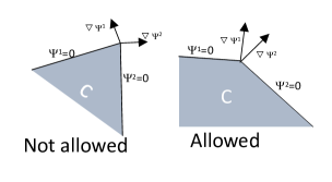
Figure 1: Examples of two diferent sets $C$. On the left size, a set that does not satisfies (2.2). On the right side, the set $C$ is nonsmooth and it fulfils (2.2).

On the other hand, (2.3) guarantees that the Gramian matrix of the gradients of the functions taking values near the boundary of $C(t)$ is diagonally dominant and, hence, the gradients are linearly independent.

In many situations, as in the example we present in the last section, we can guarantee the fulfillment of (A1), in particular (2.4), replacing the function $\psi^{i}$ by

$$\tilde{\psi}^{i}(t,x)=h\circ\psi^{i}(t,x),$$ (2.5)

where

$$h(z)=\left\{\begin{array}[]{lcl}z&\text{ if}&z>-\beta,\\ h_{s}(z)&\text{ if}&-2\beta\leq z\leq-\beta,\\ -2\beta&\text{ if}&z<-2\beta,\end{array}\right.$$

Here, $h$ is an $C^{2}$ function, with $h_{s}$ an increasing function defined on $[-2\beta,-\beta]$. For example, $h$ may be a cubic polinomial with positive derivative on the interval $]-2\beta,-\beta[$. For all $t\in[0,T]$, set

$$\tilde{C}(t):=\left\{x\in R:~{}\tilde{\psi}^{i}(t,x)\leq 0,~{}i=1,\ldots,I\right\}.$$

It is then a simple matter to see that

$$C(t)=\tilde{C}(t)\text{ for all }t\in[0,T].$$

and that the functions $\tilde{\psi}^{i}(\cdot)$ satisfy the assumption (A1).

The assumption that the graph of $C(\cdot)$ is compact and contained in the interior of a ball is introduced to avoid technicalities in our forthcoming analysis. In applied problems, this may be easily side tracked by considering the intersection of the graph of $C(\cdot)$ with a tube around the optimal trajectory.

We now proceed introducing an approximation family of controlled systems to (1.1). Let $x(\cdot)$ be a solution to the differential inclusion

$$\dot{x}(t)\in f(t,x(t),U)-N_{C(t)}(x(t)).$$

Under our assumptions, measurable selection theorems assert the existence of measurable functions $u$ and $\xi^{i}$ such that $u(t)\in U$, $\xi^{i}(t)\geq 0$ a.e. $t\in[0,T]$, $\xi^{i}(t)=0$ if $\psi^{i}(t,x(t))<0$, and

$$\dot{x}(t)=f(t,x(t),u(t))-\sum_{i=1}^{I}\xi^{i}(t)\nabla_{x}\psi^{i}(t,x(t))\;{\rm a.e.}\;t\in[0,T].$$

Considering the trajectory $x$, some observations are called for. Let $\mu$ be such that

$$\max\left\{(|\nabla_{x}\psi^{i}(t,x)||f(t,x,u)|+|\partial_{t}\psi^{i}(t,x)|)+1:\right.\\[2.84526pt] \left.~{}t\in[0,T],\;u\in U,\;x\in C(t)+B_{n},\;i=1,\ldots,I\right\}\leq\mu.$$ (2.6)

The properties of the graph of $C(\cdot)$ in (A1) guarantee the existence of such maximum.

Consider now some $t$ such that, for some $j\in\{1,\ldots I\}$, $\psi^{j}(t,x(t))=0$ and $\dot{x}(t)$ exists. Since the trajectory $x$ is always in $C$, we have (see (2.2))

$$\begin{split}0&=\frac{d}{dt}\psi^{j}(t,x(t))=\langle\nabla_{x}\psi^{j}(t,x(t)),\dot{x}(t)\rangle+\partial_{t}\psi^{j}(t,x(t))\\[5.69054pt] &=\langle\nabla_{x}\psi^{j}(t,x(t)),f(t,x(t),u(t))\rangle-\xi^{j}(t)|\nabla_{x}\psi^{j}(t,x(t))|^{2}\\[5.69054pt] &-\sum_{i\in I(t,x(t))\setminus\{j\}}\xi^{i}(t)\langle\nabla_{x}\psi^{i}(t,x(t)),\nabla_{x}\psi^{j}(t,x(t))\rangle+\partial_{t}\psi^{j}(t,x(t))\\[5.69054pt] &\leq\langle\nabla_{x}\psi^{j}(t,x(t)),f(t,x(t),u(t))\rangle-\xi^{j}(t)|\nabla_{x}\psi^{j}(t,x(t))|^{2}+\partial_{t}\psi^{j}(t,x(t)),\end{split}$$

and, hence (see (2.1)),

$$\xi^{j}(t)\leq\frac{1}{|\nabla_{x}\psi^{j}(t,x(t))|^{2}}(\langle\nabla_{x}\psi^{j}(t,x(t)),f(t,x(t),u(t))\rangle+\partial_{t}\psi^{j}(t,x(t)))\leq\frac{\mu}{\eta^{2}}.$$

Define the function

$$\mu(\gamma)=\frac{1}{\gamma}\log\left(\frac{\mu}{\eta^{2}\gamma}\right),\quad\gamma>0,$$

consider a sequence $\{\sigma_{k}\}$ such that $\sigma_{k}\downarrow 0$ and choose another sequence $\{\gamma_{k}\}$ with $\gamma_{k}\uparrow+\infty$ and

$$C(t)\subset{\rm int}\>C^{k}(t)={\rm int}\>\left\{x:\psi^{i}(t,x)-\sigma_{k}\leq\mu_{k},\;i=1,\ldots,I\right\},$$

where

$$\mu_{k}=\mu(\gamma_{k}).$$

Let $x_{k}$ be a solution to the differential equation

$$\dot{x}_{k}(t)=f(t,x_{k}(t),u_{k}(t))-\sum_{i=1}^{I}\gamma_{k}e^{\gamma_{k}(\psi^{i}(t,x_{k}(t))-\sigma_{k})}\nabla_{x}\psi^{i}(t,x_{k}(t))$$ (2.7)

for some $u_{k}(t)\in U$ a.e. $t\in[0,T]$. Take any $t\in[0,T]$ such that $\dot{x}_{k}(t)$ exists and $\psi^{j}(t,x_{k}(t))-\sigma_{k}=\mu_{k}$. Assume $k$ is such that $j\in I(t,x_{k}(t))$. Then, whenever $\gamma_{k}$ is sufficiently large, we have

$$\begin{split}\frac{d}{dt}\psi^{j}(t,x_{k}(t))&=\langle\nabla_{x}\psi^{j}(t,x_{k}(t)),f(t,x_{k}(t),u_{k}(t))\rangle\\ &\hskip 28.45274pt-\gamma_{k}e^{\gamma_{k}(\psi^{j}(t,x_{k}(t))-\sigma_{k})}|\nabla_{x}\psi^{j}(t,x_{k}(t))|^{2}\\ &\hskip 8.5359pt-\sum_{i\in I(t,x_{k}(t))\setminus\{j\}}\gamma_{k}e^{\gamma_{k}(\psi^{i}(t,x_{k}(t))-\sigma_{k})}\langle\nabla_{x}\psi^{i}(t,x_{k}(t)),\nabla_{x}\psi^{j}(t,x_{k}(t))\rangle\\ &\hskip 8.5359pt-\sum_{i\not\in I(t,x_{k}(t))}\gamma_{k}e^{\gamma_{k}(\psi^{i}(t,x_{k}(t))-\sigma_{k})}\langle\nabla_{x}\psi^{i}(t,x_{k}(t)),\nabla_{x}\psi^{j}(t,x_{k}(t))\rangle\\ &\hskip 8.5359pt+\partial_{t}\psi^{j}(t,x_{k}(t))\\ &\leq\langle\nabla_{x}\psi^{j}(t,x_{k}(t)),f(t,x_{k}(t),u_{k}(t))\rangle\\ &\hskip 8.5359pt-\gamma_{k}e^{\gamma_{k}(\psi^{j}(t,x_{k}(t))-\sigma_{k})}|\nabla_{x}\psi^{j}(t,x_{k}(t))|^{2}\\ &\hskip 8.5359pt-\sum_{i\not\in I(t,x_{k}(t))}\gamma_{k}e^{\gamma_{k}(\psi^{i}(t,x_{k}(t))-\sigma_{k})}\langle\nabla_{x}\psi^{i}(t,x_{k}(t)),\nabla_{x}\psi^{j}(t,x_{k}(t))\rangle\\ &\hskip 8.5359pt+\partial_{t}\psi^{j}(t,x_{k}(t))\\ &\leq\langle\nabla_{x}\psi^{j}(t,x_{k}(t)),f(t,x_{k}(t),u_{k}(t))\rangle\\ &\hskip 8.5359pt-\gamma_{k}e^{\gamma_{k}(\psi^{j}(t,x_{k}(t))-\sigma_{k})}|\nabla_{x}\psi^{j}(t,x_{k}(t))|^{2}\\ &\hskip 8.5359pt+\sum_{i\not\in I(t,x_{k}(t))}\gamma_{k}e^{\gamma_{k}(-{\color[rgb]{1,0,0}2}\beta-\sigma_{k})}|\langle\nabla_{x}\psi^{i}(t,x_{k}(t)),\nabla_{x}\psi^{j}(t,x_{k}(t))\rangle|\\ &\hskip 8.5359pt+\partial_{t}\psi^{j}(t,x_{k}(t))\\ &\leq\mu-\frac{1}{2}-\eta^{2}\gamma_{k}e^{\gamma_{k}\mu_{k}}\\ &=-\frac{1}{2}.\end{split}$$

Above, we have used the definition of $\mu$ and the inequality

$$\sum_{i\not\in I(t,x_{k}(t))}\gamma_{k}e^{\gamma_{k}(-{\color[rgb]{1,0,0}2}\beta-\sigma_{k})}|\langle\nabla_{x}\psi^{i}(t,x_{k}(t)),\nabla_{x}\psi^{j}(t,x_{k}(t))\rangle|\leq\frac{1}{2},$$

which holds for $\gamma_{k}$ sufficiently large.

Now, if $x_{k}(0)\in C^{k}(0)$, we assure that $x_{k}(t)\in C^{k}(t)$, for all $t\in[0,T]$, and

$$\gamma_{k}e^{\gamma_{k}(\psi^{j}(t,x_{k}(t))-\sigma_{k})}\leq\gamma_{k}e^{\gamma_{k}\mu_{k}}=\frac{\mu}{\eta^{2}}.$$ (2.8)

It follows that, for $k$ sufficienttly large, we have

$$|\dot{x}_{k}(t)|\leq({\rm const}).$$

We are now a in position to state and prove our first result, Theorem 2.2 below. This is in the vein of Theorem 4.1 in [23] (see also Lemma 1 in [10] when $\psi$ is independent of $t$ and convex) deviating from it in so far as the approximating sequence of control systems (2.7) differs from the one introduced in [10]. The proof of Theorem 2.2 relies on (2.8).

Theorem 2.2

Let $\{(x_{k},u_{k})\}$, with $u_{k}(t)\in U$ a.e., be a sequence of solutions of Cauchy problems

$$\left\{\begin{array}[]{rcl}\dot{x}_{k}(t)&=&f(t,x_{k}(t),u_{k}(t))-\displaystyle\sum_{i=1}^{I}\gamma_{k}e^{\gamma_{k}(\psi^{i}(t,x_{k}(t))-\sigma_{k})}\nabla_{x}\psi^{i}(t,x_{k}(t)),\\[5.69054pt] x_{k}(0)&=&b_{k}\in C^{k}(0).\end{array}\right.$$ (2.9)

If $b_{k}\rightarrow x_{0}$, then there exists a subsequence $\{x_{k}\}$ (we do not relabel) converging uniformly to $x$, a unique solution to the Cauchy problem

$$\dot{x}(t)\in f(t,x(t),u(t))-N_{C(t)}(x(t)),\;\;\;x(0)=x_{0},$$ (2.10)

where $u$ is a measurable function such that $u(t)\in U$ a.e. $t\in[0,T]$.

If, moreover, all the controls $u_{k}$ are equal, i.e., $u_{k}=u$, then the subsequence converges to a unique solution of (2.10), i.e., any solution of

$$\dot{x}(t)\in f(t,x(t),U)-N_{C(t)}(x(t)),\;\;\;x(0)=x_{0}\in C(0)$$ (2.11)

can be approximated by solutions of (2.9).

Proof Consider the sequence $\{x_{k}\}$, where $(x_{k},u_{k})$ solves (2.9). Recall that $x_{k}(t)\in C^{k}(t)$ for all $t\in[0,T]$, and

$$|\dot{x}_{k}(t)|\leq({\rm const})\;\;\;{\rm and}\;\;\;\xi_{k}^{i}(t)=\gamma_{k}e^{\gamma_{k}(\psi^{i}(t,x_{k}(t))-\sigma_{k})}\leq({\rm const}).$$ (2.12)

Then there exist subsequences (we do not relabel) weakly-$*$ converging in $L^{\infty}$ to some $v$ and $\xi^{i}$. Hence

$$x_{k}(t)=x_{0}+\int_{0}^{t}\dot{x}_{k}(s)ds\longrightarrow x(t)=x_{0}+\int_{0}^{t}v(s)ds,~{}\forall~{}t\in[0,T],$$

for an absolutely continuous function $x$. Obviously, $x(t)\in C(t)$ for all $t\in[0,T]$. Considering the sequence $\{x_{k}\}$, recall that

$$\dot{x}_{k}(t)\in f(t,x_{k}(t),U)-\sum_{i=1}^{I}\xi_{k}^{i}(t)\nabla_{x}\psi^{i}(t,x_{k}(t)).$$ (2.13)

Inclusion (2.13) is equivalent to

$$\langle z,\dot{x}_{k}(t)\rangle\leq S(z,f(t,x_{k}(t),U))-\sum_{i=1}^{I}\xi_{k}^{i}(t)\langle z,\nabla_{x}\psi^{i}(t,x_{k}(t))\rangle,\;\;\;\forall\>z\in R^{n}.$$

Integrating this inequality, we get

$$\left\langle z,\frac{x_{k}(t+\tau)-x_{k}(t)}{\tau}\right\rangle\\ \leq\frac{1}{\tau}\int_{t}^{t+\tau}\left(S(z,f(s,x_{k}(s),U))-\sum_{i=1}^{I}\xi_{k}^{i}(s)\langle z,\nabla_{x}\psi^{i}(s,x_{k}(s))\rangle\right)ds\\ =\frac{1}{\tau}\int_{t}^{t+\tau}\left(S(z,f(s,x_{k}(s),U))-\sum_{i=1}^{I}\xi_{k}^{i}(s)\langle z,\nabla_{x}\psi^{i}(s,x(s))\rangle\right.\\ +\left.\sum_{i=1}^{I}\xi_{k}^{i}(s)\langle z,\nabla_{x}\psi^{i}(s,x(s))-\nabla_{x}\psi^{i}(s,x_{k}(s))\rangle\right)ds.$$ (2.14)

Passing to the limit as $k\rightarrow\infty$, we obtain

$$\left\langle z,\frac{x(t+\tau)-x(t)}{\tau}\right\rangle\\ \leq\frac{1}{\tau}\int_{t}^{t+\tau}\left(S(z,f(s,x(s),U))-\sum_{i=1}^{I}\xi^{i}(s)\langle z,\nabla_{x}\psi^{i}(s,x(s))\rangle\right)ds.$$ (2.15)

Let $t\in[0,T]$ be a Lebesgue point of $x$ and $\xi$. Passing in the last inequality to the limit as $\tau\downarrow 0$, it leads to

$$\langle z,\dot{x}(t)\rangle\leq S(z,f(t,x(t),U))-\sum_{i=1}^{I}\xi^{i}(t)\langle z,\nabla_{x}\psi^{i}(t,x(t))\rangle.$$

Since $z\in R^{n}$ is an arbitrary vector and the set $f(t,x(t),U)$ is convex, we conclude that

$$\dot{x}(t)\in f(t,x(t),U)-\sum_{i=1}^{I}\xi^{i}(t)\nabla_{x}\psi^{i}(t,x(t)).$$

By the Filippov lemma there exists a measurable control $u(t)\in U$ such that

$$\dot{x}(t)=f(t,x(t),u(t))-\sum_{i=1}^{I}\xi^{i}(t)\nabla_{x}\psi^{i}(t,x(t)).$$

Furthermore, observe that $\xi^{i}$ is zero if $\psi^{i}(t,x(t))<0$. If for some $u$ such that $u(t)\in U$ a.e., $u_{k}=u$ for all $k$, then the sequence $x_{k}$ converges to the solution of

$$\dot{x}(t)=f(t,x(t),u(t))-\sum_{i=1}^{I}\xi^{i}(t)\nabla_{x}\psi^{i}(t,x(t)).$$

Indeed, to see this, it suffices to pass to the limit as $k\rightarrow\infty$ and then as $\tau\downarrow 0$, in the equality

$$\frac{x_{k}(t+\tau)-x_{k}(t)}{\tau}=\frac{1}{\tau}\int_{t}^{t+\tau}\left(f(s,x_{k}(s),u(s))-\sum_{i=1}^{I}\xi_{k}^{i}(s)\nabla_{x}\psi^{i}(s,x_{k}(s))\right)ds.$$

We now prove the uniqueness of the solution. We follow the proof of Theorem 4.1 in [23]. Notice, however, that we now consider a special case and not the general case treated in [23]. Suppose that there exist two different solutions of (2.10): $x_{1}$ and $x_{2}$. We have

$$\frac{1}{2}\frac{d}{dt}|x_{1}(t)-x_{2}(t)|^{2}=\langle x_{1}(t)-x_{2}(t),\dot{x}_{1}(t)-\dot{x}_{2}(t)\rangle\\ =\langle x_{1}(t)-x_{2}(t),f(t,x_{1}(t),u(t))-f(t,x_{2}(t),u(t))\rangle\\ -\left\langle x_{1}(t)-x_{2}(t),\sum_{i=1}^{I}\xi_{1}^{i}(t)\nabla\psi^{i}(t,x_{1}(t))-\sum_{i=1}^{I}\xi_{2}^{i}(t)\nabla\psi^{i}(t,x_{2}(t))\right\rangle.$$ (2.16)

If, for all $i$, $\psi^{i}(t,x_{1}(t))<0$ and $\psi^{i}(t,x_{2}(t))<0$, then $\xi_{1}^{i}(t)=\xi_{2}^{i}(t)=0$ and we obtain

$$\frac{1}{2}\frac{d}{dt}|x_{1}(t)-x_{2}(t)|^{2}\leq L_{f}|x_{1}(t)-x_{2}(t)|^{2}.$$

Suppose that $\psi^{j}(t,x_{1}(t))=0$. Then by the Taylor formula we get

$$\psi^{j}(t,x_{2}(t))=\psi^{j}(t,x_{1}(t))+\langle\nabla_{x}\psi^{j}(t,x_{1}(t)),x_{2}(t)-x_{1}(t)\rangle\\ +\frac{1}{2}\langle x_{2}(t)-x_{1}(t),\nabla_{x}^{2}\psi^{j}(t,\theta x_{2}(t)+(1-\theta)x_{1}(t))(x_{2}(t)-x_{1}(t))\rangle,$$ (2.17)

where $\theta\in[0,1]$. Since $\psi^{j}(t,x_{2}(t))\leq 0$, we have

$$\langle\nabla_{x}\psi^{j}(t,x_{1}(t)),x_{2}(t)-x_{1}(t)\rangle\\ \leq-\frac{1}{2}\langle x_{2}(t)-x_{1}(t),\nabla_{x}^{2}\psi^{j}(t,\theta x_{2}(t)+(1-\theta)x_{1}(t))(x_{2}(t)-x_{1}(t))\rangle\\ \leq({\rm const})|x_{1}(t)-x_{2}(t)|^{2}.$$ (2.18)

Now, if $\psi^{j}(t,x_{2}(t))=0$, we deduce in the same way that

$$\langle\nabla_{x}\psi^{j}(t,x_{2}(t)),x_{1}(t)-x_{2}(t)\rangle\leq({\rm const})|x_{1}(t)-x_{2}(t)|^{2}.$$

Thus we have

$$\frac{1}{2}\frac{d}{dt}|x_{1}(t)-x_{2}(t)|^{2}\leq({\rm const})|x_{1}(t)-x_{2}(t)|^{2}.$$

Hence $|x_{1}(t)-x_{2}(t)|=0$. $\Box$

3 Approximating Family of Optimal Control Problems

In this section we define an approximating family of optimal control problems to $(P)$ and we state the corresponding necessary conditions.

Let $(\hat{x},\hat{u})$ be a global solution to $(P)$ and consider sequences $\{\gamma_{k}\}$ and $\{\sigma_{k}\}$ as defined above. Let $\hat{x}_{k}(\cdot)$ be the solution to

$$\left\{\begin{array}[]{rcl}&&\dot{x}(t)=f(t,x(t),\hat{u}(t))-\displaystyle\sum_{i=1}^{I}\gamma_{k}e^{\gamma_{k}(\psi^{i}(t,x(t))-\sigma_{k})}\nabla_{x}\psi^{i}(t,x(t)),\\ &&x(0)=\hat{x}(0).\end{array}\right.$$ (3.1)

Set $\epsilon_{k}=|\hat{x}_{k}(T)-\hat{x}(T)|$. It follows from Theorem 2.2 that $\epsilon_{k}\downarrow 0$. Take $\alpha>0$ and define the problem

$$(P_{k}^{\alpha})\left\{\begin{array}[]{l}\mbox{Minimize }\;\phi(x(T))+|x(0)-\hat{x}(0)|^{2}+\alpha\displaystyle\int_{0}^{T}|u(t)-\hat{u}(t)|dt\\[5.69054pt] \mbox{over processes $(x,u)$ such that }\\[5.69054pt] \hskip 22.76219pt\dot{x}(t)=f(t,x(t),u(t))-\displaystyle\sum_{i=1}^{I}\nabla_{x}e^{\gamma_{k}(\psi^{i}(t,x(t))-\sigma_{k})}\hskip 5.69046pt\mbox{a.e.}\ \ t\in[0,T],\\[5.69054pt] \hskip 22.76219ptu(t)\in U~{}~{}~{}~{}\mbox{a.e.}\ \ t\in[0,T],\\[5.69054pt] \hskip 22.76219ptx(0)\in C_{0},~{}~{}x(T)\in C_{T}+\epsilon_{k}B_{n},\end{array}\right.$$

Clearly, the problem $(P_{k}^{\alpha})$ has admissible solutions. Consider the space

$$W=\{(c,u)\mid c\in C_{0},\;u\in L^{\infty}\;{\rm with}\;u(t)\in U\}$$

and the distance

$$d_{W}((c_{1},u_{1}),(c_{2},u_{2}))=|c_{1}-c_{2}|+\int_{0}^{T}|u_{1}(t)-u_{2}(t)|dt.$$

Endowed with $d_{W}$, $W$ is a complete metric space. Take any $(c,u)\in W$ and a solution $y$ to the Cauchy problem

$$\left\{\begin{array}[]{rcl}\dot{y}(t)&=&f(t,y(t),u(t))-\displaystyle\sum_{i=1}^{I}\nabla_{x}e^{\gamma_{k}(\psi^{i}(t,y(t))-\sigma_{k})}\hskip 5.69046pt\mbox{a.e.}\ \ t\in[0,T],\\[5.69054pt] y(0)&=&c.\end{array}\right.$$

Under our assumptions, the function

$$(c,u)~{}\rightarrow~{}\phi(y(T))+|c-\hat{x}(0)|^{2}+\alpha\int_{0}^{T}|u-\hat{u}|~{}dt$$

is continuous on $(W,d_{W})$ and bounded below. Appealing to Ekeland’s Theorem we deduce the existence of a pair $(x_{k},u_{k})$ solving the following problem

$$(AP_{k})\left\{\begin{array}[]{l}\mbox{Minimize }\;\Phi(x,{u})=\phi(x(T))+|x(0)-\hat{x}(0)|^{2}+\alpha\displaystyle\int_{0}^{T}|u(t)-\hat{u}(t)|dt\\[8.53581pt] \qquad\qquad+\epsilon_{k}\left(|x(0)-x_{k}(0)|+\displaystyle\int_{0}^{T}|u(t)-u_{k}(t)|dt\right),\\[5.69054pt] \mbox{over processes $(x,u)$ such that }\\[5.69054pt] \hskip 22.76219pt\dot{x}(t)=f(t,x(t),u(t))-\displaystyle\sum_{i=1}^{I}\nabla_{x}e^{\gamma_{k}(\psi^{i}(t,x(t))-\sigma_{k})}\hskip 5.69046pt\mbox{a.e.}\ \ t\in[0,T],\\[5.69054pt] \hskip 22.76219ptu(t)\in U~{}~{}~{}~{}\mbox{a.e.}\ \ t\in[0,T],\\[5.69054pt] \hskip 22.76219ptx(0)\in C_{0},~{}~{}x(T)\in C_{T}+\epsilon_{k}B_{n},\end{array}\right.$$

Lemma 3.1

Take $\gamma_{k}\to\infty$, $\sigma_{k}\to 0$ and $\epsilon_{k}\to 0$ as defined above. For each $k$, let $(x_{k},u_{k})$ be the solution to $(AP_{k})$. Then there exists a subsequence (we do not relabel) such that

$$u_{k}(t)\rightarrow\hat{u}(t)~{}{a.e.},\quad x_{k}\rightarrow\hat{x}\;\rm{uniformly}\;in\;[0,T].$$

Proof We deduce from Theorem 2.2 that $\{x_{k}\}$ uniformly converges to an admissible solution $\tilde{x}$ to $(P)$. Since $U$ and $C_{0}$ are compact, we have $U\subset KB_{m}$ and $C_{0}\subset KB_{n}$. Without loss of generality, $u_{k}$ weakly-$*$ converges to a function $\tilde{u}\in L_{\infty}([0,T],U)$. Hence it weakly converges to $\tilde{u}$ in $L_{1}$. From optimality of the processes $(x_{k},u_{k})$ we have

$$\phi(x_{k}(T))+|x_{k}(0)-\hat{x}(0)|^{2}+\alpha\int_{0}^{T}|u_{k}(t)-\hat{u}(t)|dt$$

$$\leq\phi(\hat{x}_{k}(T))+\epsilon_{k}\left(|\hat{x}_{k}(0)-x_{k}(0)|+\int_{0}^{T}|u_{k}(t)-\hat{u}(t)|dt\right)$$

$$\leq\phi(\hat{x}_{k}(T))+2K(1+T)\epsilon_{k}.$$

Since $(\hat{x},\hat{u})$ is a global solution of the problem, passing to the limit, we get

$$\phi(\tilde{x}(T))+|\tilde{x}(0)-\hat{x}(0)|^{2}+\alpha\int_{0}^{T}|\tilde{u}(t)-\hat{u}(t)|dt$$

$$\leq\lim_{k\rightarrow\infty}(\phi(x_{k}(T))+|x_{k}(0)-\hat{x}(0)|^{2})+\alpha\liminf_{k\rightarrow\infty}\int_{0}^{T}|u_{k}(t)-\hat{u}(t)|dt$$

$$\leq\lim_{k\rightarrow\infty}\phi(\hat{x}_{k}(T))=\phi(\hat{x}(T))\leq\phi(\tilde{x}(T)).$$

Hence $\tilde{x}(0)=\hat{x}(0)$, $\tilde{u}=\hat{u}$ a.e., and $u_{k}$ converges to $\hat{u}$ in $L_{1}$, and some subsequence converges to $\hat{u}$ almost everywhere (we do not relabel). $\Box$

We now finish this section with the statement of the optimality necessary conditions for the family of problems $(AP_{k})$. These can be seen as a direct consequence of Theorem 6.2.1 in [22].

Proposition 3.2

For each k, let $(x_{k},u_{k})$ be a solution to $(AP_{k})$. Then there exist absolutely continous functions $p_{k}$ and scalars $\lambda_{k}\geq 0$ such that

• (nontriviality condition)

  $$\lambda_{k}+|p_{k}(T)|=1,$$ (3.2)

• (adjoint equation)

  $$\begin{array}[]{c}\dot{p}_{k}={\color[rgb]{1,0,0}-}(\nabla_{x}f_{k})^{*}p_{k}+\sum_{i=1}^{I}\gamma_{k}e^{\gamma_{k}(\psi_{k}^{i}-\sigma_{k})}\nabla^{2}_{x}\psi_{k}^{i}p_{k}\\[5.69054pt] +\sum_{i=1}^{I}\gamma_{k}^{2}e^{\gamma_{k}(\psi_{k}^{i}-\sigma_{k})}\nabla_{x}\psi_{k}^{i}\langle\nabla_{x}\psi_{k}^{i},p_{k}\rangle,\end{array}$$ (3.3)

  where the superscript $*$ stands for transpose,

• (maximization condition)

  $$\max_{u\in U}\left\{\langle f(t,x_{k},u),p_{k}\rangle-\alpha\lambda_{k}|u-\hat{u}|-\epsilon_{k}\lambda_{k}|u-u_{k}|\right\}$$ (3.4)

  is attained at $u_{k}(t)$, for almost every $t\in[0,T]$,

• (transversality condition)

  $$(p_{k}(0),-p_{k}(T))\in\lambda_{k}\left(2(x_{k}(0)-\hat{x}(0))+\epsilon_{k}B_{n},\partial\phi(x_{k}(T))\right)$$

  $$+N_{C_{0}}(x_{k}(0))\times N_{C_{T}+\epsilon_{k}B_{n}}(x_{k}(T)).\hskip 28.45274pt$$ (3.5)

To simplify the notation above, we drop the $t$ dependance in $p_{k}$, $\dot{p}_{k}$, $x_{k}$, $u_{k}$, $\hat{x}$ and $\hat{u}$. Moreover, in (b), we write $\psi_{k}$ instead of $\psi(t,x_{k}(t))$, $f_{k}$ instead of $f(t,x_{k}(t),u_{k}(t))$. The same holds for the derivatives of $\psi$ and $f$.

4 Maximum Principle for $(P)$

In this section, we establish our main result, a Maximum Principle for $(P)$. This is done by taking limits of the conclusions of Proposition 3.2, following closely the analysis done in the proof of [10, Theorem 2].

Observe that

$$\begin{split}\frac{1}{2}\frac{d}{dt}|p_{k}(t)|^{2}&=-\langle\nabla_{x}f_{k}p_{k},p_{k}\rangle+\sum_{i=1}^{I}\gamma_{k}e^{\gamma_{k}(\psi_{k}^{i}-\sigma_{k})}\langle\nabla_{x}^{2}\psi_{k}^{i}p_{k},p_{k}\rangle\\ &\hskip 28.45274pt+\sum_{i=1}^{I}\gamma_{k}^{2}e^{\gamma_{k}(\psi_{k}^{i}-\sigma_{k})}\langle\nabla_{x}\psi_{k}^{i},p_{k}\rangle^{2}\\ &\geq-\langle\nabla_{x}f_{k}p_{k},p_{k}\rangle+\sum_{i=1}^{I}\gamma_{k}e^{\gamma_{k}(\psi_{k}^{i}-\sigma_{k})}\langle\nabla_{x}^{2}\psi_{k}^{i}p_{k},p_{k}\rangle\\ &\geq\ -M|p_{k}|^{2}+\sum_{i=1}^{I}\gamma_{k}e^{\gamma_{k}(\psi_{k}^{i}-\sigma_{k})}\langle\nabla_{x}^{2}\psi_{k}^{i}p_{k},p_{k}\rangle,\end{split}$$

where $M$ is the constant of (A2). Taking into account hypothesis (A1) and (2.8) we deduce the existence of a constant $K_{0}>0$ such that

$$\frac{1}{2}\frac{d}{dt}|p_{k}(t)|^{2}\geq-K_{0}|p_{k}{\color[rgb]{0,0,1}(t)}|^{2}.$$

This last inequality leads to

$$|p_{k}(t)|^{2}\ \leq\ e^{2K_{0}(T-t)}|p_{k}(T)|^{2}\leq\ e^{2K_{0}T}|p_{k}(T)|^{2}.$$

Since, by (a) of Proposition 3.2, $|p_{k}(T)|\leq 1$, we deduce from the above that there exists $M_{0}>0$ such that

$$|p_{k}(t)|\ \leq M_{0}.$$ (4.1)

Now, we claim that the sequence $\{\dot{p}_{k}\}$ is uniformly bounded in $L^{1}$. To prove our claim, we need to establish bounds for the three terms in (3.3). Following [10] and [14], we start by deducing some inequalities that will be of help.

Denote $I_{k}=I(t,x_{k}(t))$ and $S_{k}^{j}={\rm sign}\left(\langle\nabla_{x}\psi_{k}^{j},p_{k}\rangle\right)$. We have

$$\begin{split}\sum_{j=1}^{I}\frac{d}{dt}&\left|\langle\nabla_{x}\psi_{k}^{j},p_{k}\rangle\right|\\ &=\sum_{j=1}^{I}\left(\langle\nabla^{2}_{x}\psi_{k}^{j}\dot{x}_{k},p_{k}\rangle+\langle\partial_{t}\nabla_{x}\psi_{k}^{j},p_{k}\rangle+\langle\nabla_{x}\psi_{k}^{j},\dot{p}_{k}\rangle\right)\,S_{k}^{j}\\ &=\sum_{j=1}^{I}\left(\langle p_{k},\nabla^{2}_{x}\psi_{k}^{j}f_{k}\rangle-\sum_{i=1}^{I}\gamma_{k}e^{\gamma_{k}(\psi_{k}^{i}-\sigma_{k})}\langle p_{k},\nabla^{2}\psi_{k}^{j}\nabla_{x}\psi_{k}^{i}\rangle\right)S_{k}^{j}\\ &\hskip 28.45274pt+\sum_{j=1}^{I}\left(\langle\partial_{t}\nabla_{x}\psi_{k}^{j},p_{k}\rangle-\langle\nabla_{x}\psi_{k}^{j},(\nabla_{x}f_{k})^{*}p_{k}\rangle\right)S_{k}^{j}\\ &\hskip 28.45274pt+\sum_{j=1}^{I}\left(\sum_{i=1}^{I}\gamma_{k}e^{\gamma_{k}(\psi_{k}^{i}-\sigma_{k})}\langle\nabla_{x}\psi_{k}^{j},\nabla^{2}_{x}\psi_{k}^{i}p_{k}\rangle\right)S_{k}^{j}\\ &\hskip 28.45274pt+\sum_{i=1}^{I}\sum_{j=1}^{I}\gamma_{k}^{2}e^{\gamma_{k}(\psi_{k}^{i}-\sigma_{k})}\langle\nabla_{x}\psi_{k}^{j},\nabla_{x}\psi_{k}^{i}\rangle\langle\nabla_{x}\psi_{k}^{i},p_{k}\rangle S_{k}^{j}\end{split}$$

Observe that (see (2.3) and (2.4))

$$\sum_{i=1}^{I}\sum_{j=1}^{I}\gamma_{k}^{2}e^{\gamma_{k}(\psi_{k}^{i}-\sigma_{k})}\langle\nabla_{x}\psi_{k}^{j},\nabla_{x}\psi_{k}^{i}\rangle\langle\nabla_{x}\psi_{k}^{i},p_{k}\rangle S_{k}^{j}\\ =\sum_{i=1}^{I}\sum_{j\in I_{k}}\gamma_{k}^{2}e^{\gamma_{k}(\psi_{k}^{i}-\sigma_{k})}\langle\nabla_{x}\psi_{k}^{j},\nabla_{x}\psi_{k}^{i}\rangle\langle\nabla_{x}\psi_{k}^{i},p_{k}\rangle S_{k}^{j}\\ =\sum_{i\not\in I_{k}}\gamma_{k}^{2}e^{\gamma_{k}(\psi_{k}^{i}-\sigma_{k})}\sum_{j\in I_{k}}\langle\nabla_{x}\psi_{k}^{j},\nabla_{x}\psi_{k}^{i}\rangle\langle\nabla_{x}\psi_{k}^{i},p_{k}\rangle S_{k}^{j}\\ +\sum_{i\in I_{k}}\gamma_{k}^{2}e^{\gamma_{k}(\psi_{k}^{i}-\sigma_{k})}\left(|\nabla_{x}\psi_{k}^{i}|^{2}+\sum_{j\in I_{k}\setminus\{i\}}\langle\nabla_{x}\psi_{k}^{j},\nabla_{x}\psi_{k}^{i}\rangle S_{k}^{j}~{}S_{k}^{i}\right)|\langle\nabla_{x}\psi_{k}^{i},p_{k}\rangle|\\ =\sum_{i\in I_{k}}\gamma_{k}^{2}e^{\gamma_{k}(\psi_{k}^{i}-\sigma_{k})}\left(|\nabla_{x}\psi_{k}^{i}|^{2}+\sum_{j\in I_{k}\setminus\{i\}}\langle\nabla_{x}\psi_{k}^{j},\nabla_{x}\psi_{k}^{i}\rangle S_{k}^{j}~{}S_{k}^{i}\right)|\langle\nabla_{x}\psi_{k}^{i},p_{k}\rangle|\\ \geq\displaystyle(1-\rho)\sum_{i\in I_{k}}\gamma_{k}^{2}e^{\gamma_{k}(\psi_{k}^{i}-\sigma_{k})}|\nabla_{x}\psi_{k}^{i}|^{2}|\langle\nabla_{x}\psi_{k}^{i},p_{k}\rangle|\\ =(1-\rho)\sum_{i=1}^{I}\gamma_{k}^{2}e^{\gamma_{k}(\psi_{k}^{i}-\sigma_{k})}|\nabla_{x}\psi_{k}^{i}|^{2}|\langle\nabla_{x}\psi_{k}^{i},p_{k}\rangle|.\hskip 56.9055pt$$ (4.2)

Using this and integrating the previous equality, we deduce the existence of $M_{1}>0$ such that:

$$\int_{0}^{T}\sum_{i=1}^{I}\gamma_{k}^{2}e^{\gamma_{k}(\psi_{k}^{i}-\sigma_{k})}|\nabla_{x}\psi_{k}^{i}|^{2}|\langle\nabla_{x}\psi_{k}^{i},p_{k}\rangle|dt\leq M_{1}.$$ (4.3)

We are now in a position to show that

$$\int_{0}^{T}\sum_{i=1}^{I}\gamma_{k}^{2}e^{\gamma_{k}(\psi_{k}^{i}-\sigma_{k})}|\nabla_{x}\psi_{k}^{i}|\left|\langle\nabla_{x}\psi_{k}^{i},p_{k}\rangle\right|\ dt$$

is bounded. For simplicity, set $L_{k}^{i}(t)=\gamma_{k}^{2}e^{\gamma_{k}(\psi_{k}^{i}-\sigma_{k})}|\nabla_{x}\psi_{k}^{i}|\left|\langle\nabla_{x}\psi_{k}^{i},p_{k}\rangle\right|$. Notice that

$$\sum_{i=1}^{I}\int_{0}^{T}L_{k}^{i}(t)dt=\displaystyle\sum_{i=1}^{I}\left\{\int_{\{t:|\nabla_{x}\psi_{k}^{i}|<\eta\}}L_{k}^{i}(t)~{}dt+\displaystyle\int_{\{t:|\nabla_{x}\psi_{k}^{i}|\geq\eta\}}L_{k}^{i}(t)dt\right\}.$$

Using (A1) and (4.3), we deduce that

$$\begin{split}\displaystyle\sum_{i=1}^{I}\int_{0}^{T}L_{k}^{i}(t)~{}dt&\leq\displaystyle\sum_{i=1}^{I}\left(\gamma_{k}^{2}e^{-\gamma_{k}(\beta+\sigma_{k})}\eta^{2}\max_{t}|p_{k}(t)|\right)\\ &\hskip 14.22636pt+\displaystyle\sum_{i=1}^{I}\left(\gamma_{k}^{2}\int_{\{t:|\nabla_{x}\psi_{k}^{i}|\geq\eta\}}e^{\gamma_{k}(\psi_{k}^{i}-\sigma_{k})}\frac{|\nabla_{x}\psi_{k}^{i}|^{2}}{|\nabla_{x}\psi_{k}^{i}|}\left|\langle\nabla_{x}\psi_{k}^{i},p_{k}\rangle\right|\ dt\right)\\[2.84526pt] &\leq\gamma_{k}^{2}I~{}e^{-\gamma_{k}(\beta+\sigma_{k})}\eta^{2}M_{0}\\ &\hskip 14.22636pt+\frac{1}{\eta}\displaystyle\sum_{i=1}^{I}\left(\int_{0}^{T}\gamma_{k}^{2}e^{\gamma_{k}(\psi_{k}^{i}-\sigma_{k})}|\nabla_{x}\psi_{k}^{i}|^{2}\left|\langle\nabla_{x}\psi_{k}^{i},p_{k}\rangle\right|\ dt\right)\\[2.84526pt] &\leq\ \eta^{2}M_{0}{\color[rgb]{0,0,1}I}+\frac{M_{1}}{\eta},\end{split}$$

for $k$ large enough. Summarizing, there exists a $M_{2}>0$ such that

$$\sum_{i=1}^{I}\gamma_{k}^{2}\int_{0}^{T}e^{\gamma_{k}(\psi_{k}^{i}-\sigma_{k})}|\nabla\psi_{k}^{i}|\left|\langle\nabla\psi_{k}^{i},p_{k}\rangle\right|\ dt\ \ \leq M_{2}.$$ (4.4)

Mimicking the analysis conducted in Step 1, b) and c) of the proof of Theorem 2 in [10] and taking into account (b) of Proposition 3.2 we conclude that there exist constants $N_{1}>0$ such that

$$\int_{0}^{T}\left|\dot{p}_{\gamma_{k}}(t)\right|dt\leq N_{1},$$ (4.5)

for $k$ sufficiently large, proving our claim.

Before proceeding, observe that it is a simple matter to assert the existence of a constant $N_{2}$ such that

$$\sum_{i=1}^{I}\int_{0}^{T}\gamma_{k}^{2}e^{\gamma_{k}(\psi_{k}^{i}-\sigma_{k})}|\langle\nabla\psi_{k}^{i},p_{\gamma_{k}}\rangle|dt\leq N_{2}.$$ (4.6)

This inequality will be of help in what follows.

Let us now recall that

$$\xi_{k}^{i}(t)=\gamma_{k}e^{\gamma_{k}(\psi^{i}(t,x_{k}(t))-\sigma_{k})}$$

and that the second inequality in (2.12) holds. We turn to the analysis of Step 2 in the proof of Theorem 2 in [10] (see also [14]). Adapting those arguments, we can conclude the existence of some function $p\in BV([0,T],R^{n})$ and, for $i=1,\ldots,I$, functions $\xi^{i}\in L^{\infty}([0,T],R)$ with $\xi^{i}(t)\geq 0\ \mbox{ a. e. }t$, $\xi^{i}(t)=0,\ t\in I_{b}^{i}$, where

$$I_{b}^{i}=\left\{t\in[0,T]:~{}\psi^{i}(t,\hat{x}(t))<0\right\},$$

and finite signed Radon measures $\eta^{i}$, null in $I_{b}^{i}$, such that, for any $z\in C([0,T],R^{n})$

$$\int_{0}^{T}\langle z,dp\rangle=-\int_{0}^{T}\langle z,(\nabla\hat{f})^{*}p\rangle dt+\displaystyle\sum_{i=1}^{I}\left(\int_{0}^{T}\xi^{i}\langle z,\nabla^{2}\hat{\psi}^{i}p\rangle dt+\int_{0}^{T}\langle z,\nabla\hat{\psi}^{i}(t)\rangle d\eta^{i}\right),$$

where $\nabla\hat{\psi}^{i}(t)=\nabla\psi^{i}(t,\hat{x}(t))$. The finite signed Radon measures $\eta^{i}$ are weak-$*$ limits of

$$\gamma_{k}^{2}e^{\gamma_{k}(\psi_{k}^{i}-\sigma_{k})}\langle\nabla\psi_{k}^{i}(x_{k}(t),p_{k}(t)\rangle dt.$$

Observe that the measures

$$\langle\nabla\psi^{i}(\hat{x}(t),p(t)\rangle d\eta^{i}(t)$$ (4.7)

are nonnegative.

For each $i=1,\ldots,I$, the sequence $\xi_{k}^{i}$ is weakly-$*$ convergent in $L^{\infty}$ to $\xi^{i}\geq 0$. Following [14], we deduce from (4.6) that, for each $i=1,\ldots,I$,

$$\int_{0}^{T}|\xi^{i}\langle\nabla_{x}\hat{\psi}^{i},p\rangle|dt=\lim_{k\rightarrow\infty}\int_{0}^{T}|\xi_{k}^{i}\langle\nabla_{x}\hat{\psi}^{i},p\rangle|dt$$

$$\leq\lim_{k\rightarrow\infty}\left(\int_{0}^{T}\xi_{k}^{i}|\langle\nabla_{x}\hat{\psi}^{i},p\rangle-\langle\nabla_{x}\psi_{k}^{i},p_{k}\rangle|dt+\int_{0}^{T}\xi_{k}^{i}|\langle\nabla_{x}\psi_{k}^{i},p_{k}\rangle|dt\right)$$

$$\leq\lim_{k\rightarrow\infty}\left(\Big{|}\xi_{k}^{i}\Big{|}_{L^{\infty}}\Big{|}\langle\nabla_{x}\hat{\psi}^{i},p\rangle-\langle\nabla_{x}\psi_{k}^{i},p_{k}\rangle\Big{|}_{L^{1}}+\frac{N_{2}}{\gamma_{k}}\right)=0.$$

It turns out that

$$\xi^{i}\langle\nabla_{x}\hat{\psi}^{i},p\rangle=0\;{\rm a.e.}.$$ (4.8)

Consider now the sequence of scalars $\{\lambda_{k}\}$. It is an easy matter to show that there exists a subsequence of $\{\lambda_{k}\}$ converging to some $\lambda\geq 0$. This, together with the convergence of $p_{k}$ to $p$, allows us to take limits in (a) and (c) of Proposition 3.2 to deduce that

$$\lambda+|p(T)|=1$$

and

$$\langle p(t),f(t,\hat{x}(t),u)\rangle-\alpha\lambda|u-\hat{u}(t)|\leq\langle p(t),f(t,\hat{x}(t),\hat{u}(t))\rangle~{}\forall u\in U,\text{ a.e. }t\in[0,T].$$

It remains to take limits of the transversality conditions (d) in Proposition 3.2. First, observe that

$$C_{T}+\epsilon_{k}B_{n}=\left\{x:~{}d(x,C_{T})\leq\epsilon_{k}\right\}.$$

From the basic properties of the Mordukhovich normal cone and subdifferential (see [19], section 1.3.3) we have

$$N_{C_{T}+\epsilon_{k}B_{n}}(x_{k}(T))\subset\text{ cl cone}\>\partial d(x_{k}(T),C_{T})$$

and

$$N_{C_{T}}(\hat{x}(T))=\text{ cl cone}\>\partial d(\hat{x}(T),C_{T}).$$

Passing to the limit as $k\to\infty$ we get

$$(p(0),-p(T))\in N_{C_{0}}(\hat{x}(0))\times N_{C_{T}}(\hat{x}(T))+\{0\}\times\lambda~{}\partial\phi(\hat{x}(T)).$$

Finally, and mimicking Step 3 in the proof of Theorem 2 in [10], we remove the dependence of the conditions on the parameter $\alpha$. This is done by taking further limits, this time considering a sequence of $\alpha_{j}\downarrow 0$.

We then summarize our conclusions in the following Theorem.

Theorem 4.1

Let $(\hat{x},\hat{u})$ be the optimal solution to $(P)$. Suppose that assumption A1–A6 are satisfied. For $i=1,\cdots,I$, set

$$I^{i}_{b}=\{t\in[0,T]:~{}\psi^{i}(t,\hat{x}(t))<0\}.$$

There exist $\lambda\geq 0$, $p\in BV([0,T],R^{n})$, finite signed Randon measures $\eta^{i}$, null in $I^{i}_{b}$, for $i=1,\cdots,I$, $\xi^{i}\in L^{\infty}([0,T],R)$, with $i=1,\cdots,I$, where $\displaystyle\xi^{i}(t)\geq 0\ \text{ a. e. }t$ and $\xi^{i}(t)=0,\ t\in I^{i}_{b},$ such that

• $\lambda+|p(T)|\neq 0$,
  

• $\dot{\hat{x}}(t)=f(t,\hat{x}(t),\hat{u}(t))-\displaystyle\sum_{i=1}^{I}\xi^{i}(t)\nabla_{x}\hat{\psi}^{i}(t),$

• for any $z\in C([0,T];R^{n})$

  $$\begin{array}[]{c}\displaystyle\int_{0}^{T}\langle z(t),dp(t)\rangle=-\displaystyle\int_{0}^{T}\langle z(t),(\nabla_{x}\hat{f}(t))^{*}p(t)\rangle dt\\[8.53581pt] \displaystyle+\sum_{i=1}^{I}\displaystyle\left(\int_{0}^{T}\xi^{i}(t)\langle z(t),\nabla^{2}_{x}\hat{\psi}^{i}(t)p(t)\rangle dt\right.\ +\displaystyle\left.\int_{0}^{T}\langle z(t),\nabla_{x}\hat{\psi}^{i}(t)\rangle d\eta_{i}\right),\end{array}$$

  where $\nabla\hat{f}(t)=\nabla_{x}f(t,\hat{x}(t),\hat{u}(t)),~{}~{}\nabla\hat{\psi}^{i}(t)=\nabla\psi^{i}(t,\hat{x}(t))$ and $\nabla^{2}\hat{\psi}^{i}(t)=\nabla^{2}\psi^{i}(t,x(t)),$
  

• $\xi_{i}(t)\langle\nabla_{x}\psi^{i}(t,\hat{x}(t)),p(t)\rangle=0$, $a.e.\,t$ for all $i=1,\ldots,I$,
  

• for all $i=1,\ldots,I$, the meaures $\langle\nabla\psi^{i}(\hat{x}(t),p(t)\rangle d\eta^{i}(t)$ are nonnegative,
  

• $\displaystyle\langle p(t),f(t,\hat{x}(t),u)\rangle\leq\langle p(t),f(t,\hat{x}(t),\hat{u}(t))\rangle$ for all $u\in U,$ $~{}a.e.\,t$,
  

• $\displaystyle\begin{array}[]{c}(p(0),-p(T))\in N_{C_{0}}(\hat{x}(0))\times N_{C_{T}}(\hat{x}(T))+\{0\}\times\lambda\partial\phi(\hat{x}(T)).\end{array}$

Noteworthy, condition e) is not considered in any of our previous works.

We now turn to the free end point case, i. e., to the problem

$$(P_{f})\left\{\begin{array}[]{l}\mbox{Minimize }\;\phi(x(T))\\[5.69054pt] \mbox{over processes $(x,u)$ such that }\\[5.69054pt] \hskip 22.76219pt\dot{x}(t)\in f(t,x(t),u(t))-N_{C(t)}(x(t)),\hskip 5.69046pt\mbox{a.e.}\ \ t\in[0,T],\\[5.69054pt] \hskip 22.76219ptu(t)\in U,\ \ \;\,\mbox{a.e.}\ \ t\in[0,T],\\[5.69054pt] \hskip 22.76219ptx(0)\in C_{0}\subset C(0).\end{array}\right.$$

Problem $(P_{f})$ differs from $(P)$ because $x(T)$ is not constrained to take values in $C_{T}$. We apply Theorem 4.1 to $(P_{f})$. Since $x(T)$ is free, we deduce from (f) in the above Theorem that $-p(T)=\lambda\partial\phi(\hat{x}(T))$. Suppose that $\lambda=0$. Then $p(T)=0$ contradicting the nontriviality condition (a) of Theorem 4.1. Without loss of generality, we then conclude that the conditions of Theorem 4.1 hold with $\lambda=1$. We summarize our findings in the following Corollary.

Corollary 4.2

Let $(\hat{x},\hat{u})$ be the optimal solution to $(P_{f})$. Suppose that assumption A1–A6 are satisfied. For $i=1,\cdots,I$, set

$$I^{i}_{b}=\{t\in[0,T]:~{}\psi^{i}(t,\hat{x}(t))<0\}.$$

There exist $p\in BV([0,T],R^{n})$, finite signed Randon measures $\eta_{i}$, null in $I^{i}_{b}$, for $i=1,\cdots,I$, $\xi^{i}\in L^{\infty}([0,T],R)$, with $i=1,\cdots,I$, where $\displaystyle\xi^{i}(t)\geq 0\ \text{ a.e. }t$ and $\xi^{i}(t)=0$ for $t\in I^{i}_{b},$ such that

• $\dot{\hat{x}}(t)=f(t,\hat{x}(t),\hat{u}(t))-\displaystyle\sum_{i=1}^{I}\xi^{i}(t)\nabla_{x}\hat{\psi}^{i}(t),$

• for any $z\in C([0,T];R^{n})$

  $$\begin{array}[]{c}\displaystyle\int_{0}^{T}\langle z(t),dp(t)\rangle=-\displaystyle\int_{0}^{T}\langle z(t),(\nabla_{x}\hat{f}(t))^{*}p(t)\rangle dt\\[8.53581pt] \displaystyle+\sum_{i=1}^{I}\displaystyle\left(\int_{0}^{T}\xi^{i}(t)\langle z(t),\nabla^{2}_{x}\hat{\psi}^{i}(t)p(t)\rangle dt\right.\ +\displaystyle\left.\int_{0}^{T}\langle z(t),\nabla_{x}\hat{\psi}^{i}(t)\rangle d\eta_{i}\right),\end{array}$$

  where $\nabla\hat{f}(t)=\nabla_{x}f(t,\hat{x}(t),\hat{u}(t)),~{}~{}\nabla\hat{\psi}^{i}(t)=\nabla\psi^{i}(t,\hat{x}(t))$ and $\nabla^{2}\hat{\psi}^{i}(t)=\nabla^{2}\psi^{i}(t,x(t)),$
  

• $\xi^{i}(t)\langle\nabla_{x}\psi^{i}(t,\hat{x}(t)),p(t)\rangle=0$ for $a.e.~{}t$ and for all $i=1,\ldots,I$,
  

• for all $i=1,\ldots,I$, the meaures $\langle\nabla\psi^{i}(\hat{x}(t),p(t)\rangle d\eta^{i}(t)$ are nonnegative,
  

• $\displaystyle\langle p(t),f(t,\hat{x}(t),u)\rangle\leq\langle p(t),f(t,\hat{x}(t),\hat{u}(t))\rangle$ for all $u\in U$, $a.e.\,t$,
  

• $\displaystyle\begin{array}[]{c}(p(0),-p(T))\in N_{C_{0}}(\hat{x}(0))\times\{0\}+\{0\}\times\partial\phi(\hat{x}(T)).\end{array}$

5 Example

Let us consider the following problem

$$\left\{\begin{array}[]{l}\mbox{Minimize }\;-x(T)\\[5.69054pt] \mbox{over processes $((x,y,z),u)$ such that }\\[5.69054pt] \hskip 22.76219pt\begin{bmatrix}\dot{x}(t)\\ \dot{y}(t)\\ \dot{z}(t)\end{bmatrix}\in\begin{bmatrix}0&\sigma&0\\ 0&0&0\\ 0&0&0\end{bmatrix}\begin{bmatrix}x\\ y\\ z\end{bmatrix}+\begin{bmatrix}0\\ u\\ 0\end{bmatrix}-N_{C}(x,y,z),\\[5.69054pt] \hskip 22.76219ptu\in[-1,1],\\[2.84526pt] \hskip 22.76219pt(x,y,z)(0)=(x_{0},y_{0},z_{0}),\\[2.84526pt] \hskip 22.76219pt(x,y,z)(T)\in C_{T},\end{array}\right.$$

where

• $0<\sigma\ll 1$,
  

• $C=\{(x,y,z)\mid x^{2}+y^{2}+(z+h)^{2}\leq 1,\;x^{2}+y^{2}+(z-h)^{2}\leq 1\},\;\;2h^{2}<1$,
  

• $(x_{0},y_{0},z_{0})\in{\rm int}C$, with $x_{0}<-\delta$, $y_{0}=0$ and $z_{0}>0$,
  

• $C_{T}=\{(x,y,z)\mid x\leq 0,\;y\geq 0,\;\delta y-y_{2}x\leq\delta y_{2}\}\cap C$, where

  $$\delta<\frac{y_{2}|x_{0}|}{y_{1}},~{}{\rm with}~{}y_{1}=\sqrt{1-x_{0}^{2}-(z_{0}+h)^{2}}\text{ and }y_{2}=\sqrt{1-h^{2}}.$$

We choose $T>0$ small and, nonetheless, sufficiently large to guarantee that, when $\sigma=0$, the system can reach the interior of $C_{T}$ but not the segment $\{(x,0,0)\mid x\in[-\delta,0]\}$. Since $\sigma$ and $T$ are small, it follows that the optimal trajectory should reach $C_{T}$ at the face $\delta y-y_{2}x=\delta y_{2}$ of $C_{T}$.

To significantly increase the value of the $x(T)$, the optimal trajectory needs to live on the boundary of $C$ for some interval of time. Then, before reaching and after leaving the boundary of $C$, the optimal trajectory lives in the interior of $C$. Since $\delta$ is small, the trajectory cannot reach $C_{T}$ from any point of the sphere $x^{2}+y^{2}+(z+h)^{2}=1$ with $z>0$. This means that, while on the boundary of $C$ the trajectory should move on the sphere $x^{2}+y^{2}+(z+h)^{2}=1$ untill reaching the plane $z=0$ and then it moves on the intersection of the two spheres.

While in the interior of $C$, the control can change sign from $-1$ to $1$ or from $1$ to $-1$. Certainly, the control should be $1$ right before reaching the boundary and $-1$ right before arriving at $C_{T}$. Changes of the control from $1$ to $-1$ or $-1$ to $1$ before reaching the boundary translate into time waste and leads to smaller values of $x(T)$. It then follows that the optimal control should be of the form

$$u(t)=\left\{\begin{array}[]{cl}1,&t\in[0,\tilde{t}],\\[2.84526pt] -1,&t\in\ ]\tilde{t},T],\end{array}\right.$$ (5.1)

for some value $\tilde{t}\in]0,T[$.

After the modification (2.5), the data of the problem satisfy the conditions under which Theorem 4.1 holds. We now show that the conclusions of Theorem 4.1 completly identify the structure (5.1) of the optimal control.

From Theorem 4.1 we deduce the existence of $\lambda\geq 0$, $p,~{}q,~{}r\in BV([0,T],R)$, finite signed Randon measures $\eta_{1}$ and $\eta_{2}$, null respectively in

$$I^{1}_{b}=\left\{(x,y,z)\mid x^{2}+y^{2}+(z+h)^{2}-1<0\right\}$$

and

$$I^{2}_{b}=\left\{(x,y,z)\mid x^{2}+y^{2}+(z-h)^{2}-1<0\right\},$$

$\xi_{i}\in L^{\infty}([0,T],R)$, with $i=1,2$, where $\displaystyle\xi_{i}(t)\geq 0\ \text{ a. e. }t$ and $\xi_{i}(t)=0,\ t\in I^{i}_{b},$ such that

$$\begin{array}[]{rl}\text{(i)}&\begin{bmatrix}\dot{x}(t)\\ \dot{y}(t)\\ \dot{z}(t)\end{bmatrix}=\begin{bmatrix}0&\sigma&0\\ 0&0&0\\ 0&0&0\end{bmatrix}\begin{bmatrix}x\\ y\\ z\end{bmatrix}+\begin{bmatrix}0\\ u\\ 0\end{bmatrix}-2\xi_{1}\begin{bmatrix}x\\ y\\ z+h\end{bmatrix}-2\xi_{2}\begin{bmatrix}x\\ y\\ z-h\end{bmatrix}\\[17.07164pt] \text{(ii)}&d\begin{bmatrix}p\\ q\\ r\end{bmatrix}=\begin{bmatrix}0&0&0\\ -\sigma&0&0\\ 0&0&0\end{bmatrix}\begin{bmatrix}p\\ q\\ r\end{bmatrix}dt\\ &\hskip 56.9055pt+2(\xi_{1}+\xi_{2})\begin{bmatrix}p\\ q\\ r\end{bmatrix}dt+2\begin{bmatrix}x\\ y\\ z+h\end{bmatrix}d\eta_{1}+2\begin{bmatrix}x\\ y\\ z-h\end{bmatrix}d\eta_{2},\\[17.07164pt] \text{(iii)}&\begin{bmatrix}p\\ q\\ r\end{bmatrix}(T)=\begin{bmatrix}\lambda\\ 0\\ 0\end{bmatrix}+\mu\begin{bmatrix}y_{2}\\ -\delta\\ 0\end{bmatrix},\text{ where }\mu\geq 0,\\[14.22636pt] \text{(iv)}&\xi_{1}(xp+yq+(z+h)r)=0,\;\xi_{2}(xp+yq+(z-h)r)=0,\\[5.69054pt] \text{(v)}&\text{the meaures }(xp+yq+(z+h)r)d\eta_{1}\text{ and }(xp+yq+(z-h)r)d\eta_{2}\\ &\hskip 14.22636pt\text{ are nonnegative,}\\[5.69054pt] \text{(vi)}&\max_{u\in[-1,1]}uq=\hat{u}q.\end{array}$$

where $\hat{u}$ is the optimal control.

Let $t_{1}$ be the instant of time when the trajectory reaches the shere $x^{2}+y^{2}+(z+h)^{2}=1$, $t_{2}$ the instant of time when the trajectory reaches the intersection of the two spheres and $t_{3}$ be the instant of time the trajectory leaves the boundary of $C$. We have $0<t_{1}<t_{2}<t_{3}<T$.

Next we show that the multiplier $q$ changes sign only once and so identifing the structure (5.1) of the optimal control in a unique way. We start by looking at the case when $t=T$. We have

$$\left[\begin{array}[]{c}p\\ q\end{array}\right](T)=\left[\begin{array}[]{c}\lambda\\ 0\end{array}\right]+\mu\left[\begin{array}[]{c}y_{2}\\ -\delta\end{array}\right].$$

Starting from $t=T$, let us go backwards in time until the instant $t_{3}$ when the trajectory leaves the boundary of $C$. If $q(T)=0$, then $p(T)=\lambda>0$ and we would have $q(t)>0$ for $t\in]t_{3},T[$ (see (ii) above), which is impossible. We then have $p(T)>0$ and $q(T)<0$ and, in $]t_{3},T[$, since $\sigma$ is small, the vector $(p(t),q(t))$ does not change much. At $t=t_{3}$, the vector $(p,q)$ has a jump and such jump can only occur along the vector $(x(t_{3}),y(t_{3}))$. Therefore, we have $p(t_{3}-0)>0$ and $q(t_{3}-0)<0$.

Let us now consider $t\in]t_{2},t_{3}[$. We have the following

1. when $t\in[t_{2},t_{3}]$, we have $z=0$;

2. condition (i) above implies that $\xi_{1}=\xi_{2}=\xi$, $\xi>0$ since, otherwise the motion along $x^{2}+y^{2}=1-h^{2}$ would not be possible;

3. from $0=\frac{d}{dt}(x^{2}+y^{2})=\sigma 2xy-8\xi x^{2}+2uy-8\xi y^{2}$ we get $\xi=\frac{\sigma xy+uy}{4(1-h^{2})}$;

4. condition (iv) implies that $r=0$ leading to $xp+yq=0$. Since $x<0$, $y>0$, then $q=0$ implies $p=0$;

5. condition (ii) implies $d\eta_{1}=d\eta_{2}=d\eta$;

6. $0=d(xp+yq)=uqdt+4(1-h^{2})d\eta$ $\Rightarrow$ $\frac{d\eta}{dt}=-\frac{uq}{4(1-h^{2})}$;

7. from the above analysis we deduce that

   $$\dot{p}=\frac{\sigma xy+uy}{(1-h^{2})}~{}p-\frac{xuq}{(1-h^{2})},$$

   $$\dot{q}=-\sigma p+\frac{\sigma xy}{(1-h^{2})}~{}q.$$

   Thus, $(p,q)$ is a solution to a linear system and it can never be equal to zero. It follows that $q$ cannot be zero because $q=0$ implies $p=0$. Since $q\neq 0$, we have $q>0$.

Let us consider the case when $t=t_{2}$. We claim that

$$(p(t_{2}-0),q(t_{2}-0))\neq(0,0).$$

Seeking a contradiction, assume that it is $(p(t_{2}-0),q(t_{2}-0))=(0,0)$. Then we have

$$(p(t_{2}+0),q(t_{2}+0))=(0,0)+(2x_{2}(t_{2}),2y_{2}(t_{2}))(d\eta_{1}+d\eta_{2})$$

and such jump has to be normal to $(x(t_{2}),y(t_{2}))$ since $r(t_{2}+0)=0$ (see (iv)). It follows that $(x^{2}(t_{2})+y^{2}(t_{2}))(d\eta_{1}+d\eta_{2})=0$ and, since $x^{2}(t_{2})+y^{2}(t_{2})>0$, we get $d\eta_{1}+d\eta_{2}=0$, proving our claim.

We now consider $t\in]t_{1},t_{2}[$. It is easy to see that $\xi_{2}=0$ and $d\eta_{2}=0$. We also deduce that

1. $0=\frac{d}{dt}(x^{2}+y^{2}+(z+h)^{2})=2\sigma xy+2uy-4\xi_{1}y^{2}-4\xi_{1}x^{2}-4\xi_{1}(z+h)^{2}$ which implies that $\xi_{1}=\frac{\sigma xy+uy}{2}$;

2. also $0=d(xp+yq+(z+h)r)=uqdt+2d\eta_{1}$ implies that $\frac{d\eta_{1}}{dt}=-\frac{uq}{2}$;

3. from the above we deduce that

   $$\dot{p}=(\sigma xy+uy)p-xuq,$$

   $$\dot{q}=-\sigma p+\sigma xyq.$$

   Thus $(p,q)$ is a solution to a linear system and never is equal to zero. Second equation implies that if $q=0$ then $\dot{q}\neq 0$. Hence $q>0$.

Now we need to consider $t=t_{1}$. We claim that

$$(p(t_{1}-0),q(t_{1}-0),r(t_{1}-0))\neq(0,0,0).$$

Let us then assume that it is $(p(t_{1}-0),q(t_{1}-0),r(t_{1}-0))=(0,0,0)$. It then follows that $(p(t_{1}+0),q(t_{1}+0),r(t_{1}+0))=(0,0,0)+(2x(t_{1})d\eta_{1},2y(t_{1})d\eta_{1},2(z(t_{1})+h)d\eta_{1})$. We now show that there is no such jump. Set $r(t_{1}-0)=r_{0}$. Then it follows from (iv) that $(x(t_{1})\cdot 0+y(t_{1})\cdot 0+(z(t_{1})+h))r_{0}=0$ which implies that $r_{0}=0$. We also have $(x^{2}(t_{1})+y^{2}(t_{1})+(z(t_{1})+h)^{2})d\eta_{1}=0$ from (v). But this implies that $d\eta_{1}=0$. Consequently, the multipliers do not exhibit a jump at $t_{1}$.

From the previous analysis we deduce that $q$ should be positive almost everywhere on the boundary. It then follows that to find the optimal solution we have to analyze admissible trajectories with the controls with the structure (5.1) and choose the optimal value of $\tilde{t}$.

Acknowledgements

The authors gratefully thank the support of Portuguese Foundation for Science and Technology (FCT) in the framework of the Strategic Funding UIDB/04650/2020.

Also we thank the support by the ERDF - European Regional Development Fund through the Operational Programme for Competitiveness and Internationalisation - COMPETE 2020, INCO.2030, under the Portugal 2020 Partnership Agreement and by National Funds, Norte 2020, through CCDRN and FCT, within projects To Chair (POCI-01-0145-FEDER-028247), Upwind (PTDC/EEI-AUT/31447/2017 - POCI-01-0145-FEDER-031447) and Systec R&D unit (UIDB/00147/2020).

References

[1] Addy K, Adly S, Brogliato B, Goeleven D, A method using the approach of Moreau and Panagiotopoulos for
the mathematical formulation of non-regular circuits in electronics, Nonlinear Anal. Hybrid Syst., vol. 1,
30–43, (2013), https://doi.org/10.1016/j.nahs.2006.04.00.
[2] Arroud C and Colombo G, Necessary conditions for a nonclassical control problem with state constraints, 20th IFAC World Congress, Toulouse, France, July 9-14, 2017, https://doi.org/10.1016/j.ifacol.2017.08.110.
[3] Arroud C and Colombo G, A maximum principle for the controlled sweeping process, Set-Valued Var. Anal 26, 607–629 (2018) DOI: 10.1007/s11228-017-0400-4.
[4] Brokate M, Krejčí P
Optimal control of ODE systems Involving a rate independent variational inequality, Disc. Cont. Dyn. Syst. Ser. B, vol. 18 (2) 331–348 (2013), doi: 10.3934/dcdsb.2013.18.331.
[5] Cao TH, Mordukhovich B,
Optimality conditions for a controlled sweeping process with applications to the crowd motion model, Disc. Cont. Dyn. Syst. Ser. B, vol. 22, 267–306 (2017).
[6] Cao TH, Colombo G, Mordukhovich B, Nguyen D., Optimization of fully controlled sweeping processes, Journal of Differential Equations,
295, 138–186 (2021) https://doi.org/10.1016/j.jde.2021.05.042
[7]
Clarke F, Optimization and nonsmooth analysis,
John Wiley, New York (1983).
[8] Colombo G, Palladino M, The minimum time function for the controlled Moreau’s sweeping process, SIAM, vol. 54, no. 4,2036– 2062 (2016), https://doi.org/10.1137/15M1043364.
[9] Colombo G,Henrion R, Hoang ND, Mordukhovich BS, Optimal control of the sweeping process over polyhedral controlled sets, Journal of Differential Equations, vol. 260, 4, 3397–3447, (2016), https://doi.org/10.1016/j.jde.2015.10.039.
[10] de Pinho MdR, Ferreira MMA, Smirnov G, Optimal Control involving Sweeping Processes, Set-Valued Var. Anal 27, 523–548, (2019), https://doi.org/10.1007/s11228-018-0501-8.
[11] de Pinho MdR, Ferreira MMA, Smirnov G, Correction to: Optimal Control Involving Sweeping Processes, Set-Valued Var. Anal 27, 1025–1027 (2019) https://doi.org/10.1007/s11228-019-00520-5.
[12] de Pinho MdR, Ferreira MMA, Smirnov G, Optimal Control with Sweeping Processes: Numerical Method, J Optim Theory Appl 185, 845– 858 (2020)
https://doi.org/10.1007/s10957-020-01670-5
[13] de Pinho MdR, Ferreira MMA, Smirnov G, Optimal Control Involving Sweeping Processes with End Point Constraints, 2021 60th IEEE Conference on Decision and Control (CDC), 2021, 96–101(2019) doi: 10.1109/CDC45484.2021.9683291
[14]de Pinho MdR, Ferreira MMA, Smirnov G, Necessary conditions for optimal control problems with sweeping systems and
end point constraints, Optimization, to appear (2022).
[15] Hermosilla C, Palladino M, Optimal Control of the Sweeping Process with a Non-Smooth Moving Set, SIAM j. Cont. Optim., to appear (2022).
[16] Kunze M, Monteiro Marques MDP, An Introduction to Moreau’s sweeping process. Impacts in Mechanical Systems, Lecture Notes in Physics, vol. 551, 1–60, (2000).
[17] Maury B, Venel J (2011), A discrete contact model for crowd motion, ESAIM: M2AN 45 1, 145–168.
[18] Moreau JJ, On unilateral constraints, friction and plasticity, In: Capriz G., Stampacchia G. (Eds.) New Variational Techniques in Mathematical Physics, CIME ciclo Bressanone 1973. Edizioni Cremonese, Rome, 171–322 (1974).
[19]
Mordukhovich B, Variational analysis and generalized differentiation. Basic Theory.
Fundamental Principles of Mathematical Sciences 330,
Springer-Verlag, Berlin (2006).
[20] Mordukhovich B,
Variational analysis and generalized differentiation II. Applications,
Fundamental Principles of Mathematical Sciences 330,
Springer-Verlag, Berlin (2006).
[21] Thibault L, Moreau sweeping process with bounded truncated retraction, J. Convex Anal, vol. 23, pp. 1051–1098 (2016).
[22] Vinter RB,
Optimal Control,
Birkhäuser, Systems and Control: Foundations and Applications, Boston MA (2000).
[23] Zeidan V, Nour C, Saoud H, A nonsmooth maximum principle for a controlled nonconvex sweeping process, Journal of Differential Equations,
vol. 269 (11), 9531–9582 (2020), https://doi.org/10.1016/j.jde.2020.06.053