Geometry-based approximation of waves in complex domains

Abstract

We consider wave propagation problems over 2-dimensional domains with piecewise-linear boundaries, possibly including scatterers. Under the assumption that the initial conditions and forcing terms are radially symmetric and compactly supported, we propose an approximation of the propagating wave as the sum of some special space-time functions. Each term in this sum identifies a particular field component, modeling the result of a single reflection or diffraction effect. We describe an algorithm for identifying such components automatically, based on the domain geometry. To showcase our proposed method, we present several numerical examples, such as waves scattering off wedges and waves propagating through a room in presence of obstacles.

Keywords: wave propagation, surrogate modeling, scattering, geometrical theory of diffraction.

AMS subject classifications: 35L05, 35Q60, 65M25, 78A45, 78M34.

1 Introduction

The discretization of numerical models for the simulation of complex phenomena results in high-dimensional systems to be solved, usually at an extremely high cost in terms of computational time and storage memory. Among these models, wave propagation problems represent an extremely interesting topic: relevant applications can be found, e.g., in the field of array imaging, where acoustic, electromagnetic, and elastic waves in scattering media are modeled by the reflectivity coefficient, which is often unknown. Some examples in this direction can be found in [1, 2, 3, 4], where inverse scattering problems are used to infer the reflectivity of one or more scatterers embedded either in a known and smooth medium, or in a randomly inhomogeneous medium. Another example of application of wave propagation problems is numerical acoustics, where the goal is to simulate the propagation of sound in a room, in presence of obstacles and walls with different absorbing and/or reflecting properties. See, e.g., [5, 6] for some frequency-domain examples of this.

Our focus here are problems in the time domain, whose numerical simulation is expensive, mainly because one needs to use both a fine spatial mesh and a carefully chosen time step in order to satisfy the CFL condition [7, 8]. In the interest of making these simulations feasible, model order reduction (MOR) [9, 10, 11] represents a promising framework, whose goal is to reduce the computational cost of solving the problem of interest.

In this context, it is well known [12] that wave propagation problems are characterized by a slowly decaying Kolmogorov $n$-width. Because of this, classical linear-subspace MOR methods are not able to reproduce the behavior of the wave propagation without relying on a very high-dimensional linear manifold. This makes linear surrogate models unappealing, since they do not yield significant speed-ups. In recent years, methods that rely on nonlinear and/or hybrid space-time approaches have been proposed. See, e.g., [13, 14, 15] and references therein.

In this work, we focus on wave propagation over 2-dimensional spatial domains, possibly including obstacles. We aim at proposing a new approximation framework, which satisfies the main goal of MOR techniques, that is, making the computational cost of the numerical simulations more feasible. We limit our investigation to domains with piecewise-linear boundaries and a constant wave speed. The initial conditions and forcing terms are assumed to be compactly supported and radially symmetric around a “source point”. Under these assumptions, and following ideas similar to those in [5, 6], we propose to construct a surrogate model for the solution of the target problem as a superposition of some special space-time terms, which we dub “field components”.

Each field component models a reflection or diffraction effect, and is characterized by:

• a space-time propagation term, related to the free-space radially symmetric solution of the wave equation;

• a spatial indicator function, determining the spatial support of each component;

• a nonlinear spatial term encoding the angular modulation of the component, which is crucial when modeling diffraction effects.

To compute the “angular modulation” term, we leverage concepts from the frequency-domain geometric theory of diffraction [16, 17]. However, in order to obtain a time-domain diffraction model that is suitable for our purposes, we first need to adapt the available results, effectively developing a novel time-domain diffraction model in the process.

The number of field components appearing in the surrogate is determined by the number of reflection and diffraction effects that are required to faithfully approximate the target wave, which ultimately depends on the geometry of the physical domain.

Among the advantages of the proposed approach, we mention the fact that each field component is separable into time-radial and angular components (in the “polar coordinates” sense). As we will see, we can leverage this to drastically reduce the computational cost and storage memory requirements of our approximation strategy.

The rest of the paper is structured as follows. In Section 1.1 we present the problem of interest. In Section 2 we introduce the main ingredients of our method, and we present our surrogate modeling algorithm. In Sections 3 and 4 we detail how we model reflection and diffraction effects, respectively. In Section 5 we present some numerical results to showcase our method. Both simple benchmarks (wedges) and more complicated tests (2D room model with scatterers) are considered. Some final considerations follow in Section 6.

1.1 Target problem

We are interested in the numerical approximation of the solution of the wave equation in complex domains. In this work, we consider 2-dimensional domains only. However, most of our discussion generalizes to 3D. We defer a discussion on this till Section 6.

We denote by $\Omega\subset\mathbb{R}^{2}$ the physical domain in which the wave equation is considered. We assume that $\Omega$ is either a closed polygon or a set-subtraction of polygons (to allow for multiply connected domains). We denote by $n_{e}$ and $n_{v}$ the number of edges and vertices of $\partial\Omega$, respectively. We study the propagation of waves in $\Omega$ over a given time interval of interest $[0,T]$. The model problem is the wave equation with constant (unit) wave speed:

$$\begin{cases}\partial_{tt}u(\bm{x},t)=\Delta u(\bm{x},t)+f(\bm{x},t)\quad&\text{for }(\bm{x},t)\in\Omega\times(0,T),\\ u(\bm{x},0)=u_{0}(\bm{x})\quad&\text{for }\bm{x}\in\Omega,\\ \partial_{t}u(\bm{x},0)=u_{1}(\bm{x})\quad&\text{for }\bm{x}\in\Omega,\\ \partial_{\nu}u(\bm{x},t)=0\quad&\text{for }(\bm{x},t)\in\partial\Omega\times(0,T],\end{cases}$$ (1)

with $\Delta$ the Laplacian operator, defined, in 2 dimensions, as $\Delta=\sum_{j=1}^{2}\partial_{x_{j}x_{j}}$. The homogeneous Neumann condition (i.e., the last equation above) models the whole boundary $\partial\Omega$ as sound-hard [7]. More generally, all or parts of $\partial\Omega$ may be modeled as sound-soft via a Dirichlet-type condition: $u(\bm{x},t)=0$.

We assume that the initial conditions $u_{0}$ and $u_{1}$, as well as the forcing term $f$, have radial symmetry around a given point. Without loss of generality, we will take such point to be the origin of $\mathbb{R}^{2}$:

$$u_{0}(\bm{x})=\eta_{0}(\left\|\bm{x}\right\|),\;u_{1}(\bm{x})=\eta_{1}(\left\|\bm{x}\right\|),\;f(\bm{x},t)=\eta_{2}(\left\|\bm{x}\right\|,t),$$ (2)

for all $(\bm{x},t)\in\Omega\times(0,T)$, with $\left\|\bm{x}\right\|^{2}=\sum_{j=1}^{2}x_{j}^{2}$. We further assume that the functions $\eta_{j}$ have compact support, namely, that there exist $R>0$ such that $\eta_{j}(\rho)=0$ for all $\rho>R$ and $j=0,1,2$. Moreover, to avoid incompatibilities with the boundary conditions, for simplicity we will only consider the situation where the supports of the functions $\eta_{j}$ are fully contained in $\Omega$.

2 Approximation framework

Before we can model boundary effects (reflection and diffraction), we need to understand how the solution $u$ would behave if no boundary were present. To this aim, we consider the wave equation in free space

$$\begin{cases}\partial_{tt}U(\bm{x},t)=\Delta U(\bm{x},t)+f(\bm{x},t)\quad&\text{for }(\bm{x},t)\in\mathbb{R}^{2}\times(0,\infty),\\ U(\bm{x},0)=u_{0}(\bm{x})\quad&\text{for }\bm{x}\in\mathbb{R}^{2},\\ \partial_{t}U(\bm{x},0)=u_{1}(\bm{x})\quad&\text{for }\bm{x}\in\mathbb{R}^{2},\end{cases}$$ (3)

which we have obtained from Eq. 1 by replacing $\Omega$ with the whole plane.

Due to radial symmetry (of the initial conditions and of the forcing term), we can recast the problem in polar coordinates. This allows us to define the free-space solution $\Psi$ in the radial coordinate, as the solution of

$$\begin{cases}\partial_{tt}\Psi(\rho,t)=\widehat{\Delta}\Psi(\rho,t)+\eta_{2}(\rho,t)\quad&\text{for }(\rho,t)\in(0,\infty)\times(0,\infty),\\ \Psi(\rho,0)=\eta_{0}(\rho)\quad&\text{for }\rho\in[0,\infty),\\ \partial_{t}\Psi(\rho,0)=\eta_{1}(\rho)\quad&\text{for }\rho\in[0,\infty),\\ \partial_{\rho}\Psi(0,t)=0\quad&\text{for }t\in(0,\infty),\end{cases}$$ (4)

where $\widehat{\Delta}$ is the Laplace operator in polar coordinates (under radial symmetry), i.e., $\widehat{\Delta}=\partial_{\rho\rho}+\frac{1}{\rho}\partial_{\rho}$, and $U(\bm{x},t)=\Psi(\left\|\bm{x}\right\|,t)$ for all $\bm{x}\in\mathbb{R}^{2}$. Note that, by the compact support of the initial conditions and of the forcing term, and by the finite (unit) speed of propagation of the wave equation, we have $\Psi(\rho,t)=0$ whenever $\rho>t+R$.

Remark 2.1.

Generally, the free-space solution $\Psi$ is not available analytically, except for very simple choices of initial conditions and forcing term. Accordingly, in most applications, the function $\Psi$ will need to be replaced with a suitable approximation. To this effect, one can discretize Eq. 4, e.g., with a finite element approximation (in space) and some timestepping scheme (in time). See Section 5 for more details on this.

Our goal is to approximate, for all $(\bm{x},t)\in\Omega\times[0,T]$, the solution $u(\bm{x},t)$ of the wave equation problem in Eq. 1 with a surrogate, defined as a sum of special functions (field components):

$$u(\bm{x},t)\approx\widetilde{u}(\bm{x},t)=\sum_{n=1}^{N}\underbrace{\Psi(\left\|\bm{x}-\bm{\xi}_{n}\right\|+r_{n},t)\mathbbm{1}_{\Omega_{n}}(\bm{x})\zeta_{n}(\bm{x}-\bm{\xi}_{n})}_{\widetilde{u}_{n}(\bm{x},t)}.$$ (5)

Therein, $\Psi$ is the above-mentioned free-space radially symmetric solution of Eq. 4, and $\mathbbm{1}_{A}$ denotes the indicator function with support $A$, i.e.,

$$\mathbbm{1}_{A}(y)=\begin{cases}1\quad&\text{if }y\in A,\\ 0\quad&\text{if }y\notin A.\end{cases}$$ (6)

Moreover, in Eq. 5, we have introduced the following quantities:

• $N$ is the number of field components used in the approximation.

• $\bm{\xi}_{n}$ is the location of the new source.

• $r_{n}\geq 0$ is a spatial delay, which is used for the synchronization of diffraction effects.

• $\Omega_{n}\subset\Omega$ is the spatial support of the field component $\widetilde{u}_{n}$.

• $\zeta_{n}:\mathbb{R}^{2}\setminus\{\bm{0}\}\to\mathbb{R}$ is a weight function describing the angular modulation. We assume $\zeta_{n}$ to be a positive-homogeneous function, i.e., $\zeta_{n}(\bm{y})=\zeta_{n}(\bm{y}/\left\|\bm{y}\right\|)$ for all $\bm{y}\in\mathbb{R}^{2}\setminus\{\bm{0}\}$.

Remark 2.2.

We refer to $\zeta_{n}$ as “angular modulation” since, in 2D, positive-homogeneity is equivalent to requiring $\zeta_{n}(\bm{y})$ to depend only on the angle between the vector $\bm{y}$ and some reference direction, e.g., the positive $x_{1}$-axis.

Note that, due to the finite speed of propagation of the free-space solution $\Psi$, we have that a generic term $\widetilde{u}_{n}(\bm{x},t)$ is zero whenever $t<\left\|\bm{x}-\bm{\xi}_{n}\right\|+r_{n}-R$, i.e., for $t$ small enough, depending on $\bm{x}$.

The number of field components $N$ in Eq. 5 will be determined based on how many boundary effects (reflections and diffractions) need to be included in $\widetilde{u}$ in order to have a good approximation of the target wave $u$. We describe a strategy for automatically identifying a good $N$ in the next section. See, e.g., Remark 2.3.

2.1 Building the low-rank skeleton

Recalling that $u$ solves the wave equation in Eq. 1 in the domain $\Omega$, we use the first term in Eq. 5, namely, $\widetilde{u}_{1}$, to approximate the outgoing component of $u$, ignoring any effect due to the boundary $\partial\Omega$, except for shadows. Then, given such $\widetilde{u}_{1}$, we use the other terms $\widetilde{u}_{2},\ldots,\widetilde{u}_{N}$ to correct this first approximation. Each extra term models a single effect due to a certain portion of the boundary, specifically, an edge (reflection off that edge) or a vertex (diffraction about that vertex).

Going back to the first field component $\widetilde{u}_{1}$, let us define it, by providing its “ingredients” $\bm{\xi}_{1}$, $r_{1}$, $\Omega_{1}$, and $\zeta_{1}$, cf. Eq. 5. We set $\bm{\xi}_{1}=\bm{0}$, the center of the initial condition, as well as $r_{1}=0$, since no delay is necessary for this first term. Then, leveraging symmetry, we set $\zeta_{1}\equiv 1$, which corresponds to the (physical) assumption that the propagation of $\widetilde{u}_{1}$ is purely radial. Finally, we set $\Omega_{1}$ (the spatial support of the first field component around $\bm{0}$) as the set of points that can be reached from $\bm{0}$ via a straight line without going outside $\partial\Omega$, i.e.,

$$\Omega_{1}=\left\{\bm{x}\in\Omega\ :\ \tau\bm{x}\in\Omega\ \ \forall 0\leq\tau\leq 1\right\}.$$ (7)

In summary, the first term of $\widetilde{u}$ is

$$\widetilde{u}_{1}(\bm{x},t)=\Psi(\left\|\bm{x}\right\|,t)\mathbbm{1}_{\Omega_{1}}(\bm{x}).$$ (8)

Then we can move to the subsequent terms $\widetilde{u}_{n}$, $n\geq 2$. Their expressions depend on our choice of reflection and diffraction modeling, and will be provided in the upcoming sections. Instead, in the rest of the present section we focus on understanding how large $N$ should be, in order for $\widetilde{u}$ to provide a faithful approximation of $u$. Equivalently, we want to count the number of times the wave gets reflected or diffracted at the boundary $\partial\Omega$. This is done incrementally, starting from the initial value $N=1$ (no boundary effects) and then updating this guess as more and more boundary effects get “discovered”.

To help us in this endeavor, we employ what we call a timetable, which, in this work, is simply a list of vectors, each with size $n_{e}+n_{v}$. (Note that similar ideas can can also be found in [5, 6, 18] and references therein.) The timetable is built incrementally starting from an empty list, appending one new vector every time a new term is added in the sum in Eq. 5, starting from $\widetilde{u}_{1}$. The entries of the $n$-th timetable vector are the waiting times before $\widetilde{u}_{n}$ comes in contact with an edge or a vertex of $\partial\Omega$. If it is impossible for $\widetilde{u}_{n}$ to “cast light” (along a straight path) onto a certain edge or vertex, then the corresponding entry in the timetable is set to $\infty$. After this, it suffices to look for the smallest not-yet-explored entry of the timetable to identify what the next term of the approximation $\widetilde{u}$ should be. Once the entry in the timetable has been explored, its value is set to $\infty$.

We start by describing how the first vector $\bm{a}_{1}\in\mathbb{R}^{n_{e}+n_{v}}$ of the timetable (corresponding to $\widetilde{u}_{1}$) is computed, and how $\bm{a}_{1}$ allows us to identify the (geometric) features of $\widetilde{u}_{2}$. The vector $\bm{a}_{1}$ can be partitioned into edges-related part (the first $n_{e}$ entries) and vertices-related part (the last $n_{v}$ entries).

• Edge times. Given a generic edge $\gamma_{j}\subset\partial\Omega$ ($j=1,\ldots,n_{e}$) belonging to the domain boundary, we define the corresponding entry of $\bm{a}_{1}$ as

  $$\left(\bm{a}_{1}\right)_{j}=\begin{cases}r_{1}+\inf\left\{\left\|\bm{x}-\bm{\xi}_{1}\right\|:\bm{x}\in\gamma_{j}\cap\overline{\Omega}_{1}\right\}&\text{if the set is non-empty},\\ \infty&\text{otherwise}.\end{cases}$$ (9)

  Note that we have taken the shortest path from $\bm{\xi}_{1}$ to $\gamma_{j}$, and that we have denoted the closure of $\Omega_{1}$ as $\overline{\Omega}_{1}$.

• Vertex times. Given a generic vertex $\bm{y}_{j}\subset\partial\Omega$ ($j=1,\ldots,n_{v}$) of the domain boundary, we set

  $$\left(\bm{a}_{1}\right)_{n_{e}+j}=\begin{cases}r_{1}+\left\|\bm{y}_{j}-\bm{\xi}_{1}\right\|\quad&\text{if }\bm{y}_{j}\in\overline{\Omega}_{1},\\ \infty\quad&\text{otherwise}.\end{cases}$$ (10)

Note that we have included the delay $r_{1}$ (which is actually zero here) as a way to streamline Eqs. 9 and 10 for the upcoming section. See Fig. 1 for a diagram showcasing these formulas.

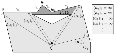
Figure 1: Computation of some timetable entries. The boundary $\partial\Omega$ has 11 sides, so that, e.g., $(\bm{a}_{1})_{14}$ is related to $\bm{y}_{3}$ and $(\bm{a}_{1})_{17}$ is related to $\bm{y}_{6}$. The shadowed area $\Omega\setminus\Omega_{1}$ is in darker grey.

The smallest entry of $\bm{a}_{1}$ is the time at which the first “boundary event” (reflection or diffraction) can happen. The index of the smallest entry tells us whether the event is a reflection (index $1\leq j\leq n_{e}$) or a diffraction (index $n_{e}+1\leq j\leq n_{e}+n_{v}$), and also what edge/vertex causes the event. From here, we use the models described in Sections 3 and 4 to build $\widetilde{u}_{2}$, by computing $\bm{\xi}_{2}$, $r_{2}$, $\Omega_{2}$, and $\zeta_{2}$.

Then, the second timetable vector $\bm{a}_{2}$ can be computed by replacing all subscripts “1” by “2” in Eqs. 9 and 10. This is followed by the construction of $\widetilde{u}_{3}$, and so on. The process continues until all not-yet-explored entries of the timetable are larger than $T+R$. Indeed, starting from this time instant, the would-be next terms of $\widetilde{u}$ do not affect the approximation anymore, since, due to the finite speed of wave propagation, they only act (on $\Omega$) after the end of the time horizon, i.e., for $t>T$. The total number of field components $N$ is simply the number of vectors in the timetable.

We summarize the overall procedure for the construction of the terms $\widetilde{u}_{n}$ in Algorithm 1. For ease of presentation, once an entry of the timetable has been explored, it is set to $\infty$ as a way for the algorithm to ignore it from that point forward.

Algorithm 1 Step-by-step construction of the surrogate model

  Set $N\leftarrow 1$, find $\Omega_{1}$ as in Eq. 7, and define $\widetilde{u}_{1}$ as in Eq. 8

  Define $\bm{a}_{1}\in\mathbb{R}^{n_{e}+n_{v}}$ using Eqs. 9 and 10

  Set $i\leftarrow 1$ and $j\leftarrow\operatorname*{arg\,min}_{j=1,\ldots,n_{e}+n_{v}}\left(\bm{a}_{1}\right)_{j}$

  while $\left(\bm{a}_{i}\right)_{j}\leq T+R$ do

     Set $\left(\bm{a}_{i}\right)_{j}\leftarrow\infty$ and $N\leftarrow N+1$

     if $j\leq n_{e}$ then

        Find $\bm{\xi}_{N}$, $r_{N}$, $\Omega_{N}$, and $\zeta_{N}$ as in Section 3 $\leftarrow$ Reflection from edge $j$

     else

        Find vertex index $j^{\prime}\leftarrow j-n_{e}$

        Find $\bm{\xi}_{N}$, $r_{N}$, $\Omega_{N}$, and $\zeta_{N}$ as in Section 4 $\leftarrow$ Diffraction from vertex $j^{\prime}$

     end if

     Define $\widetilde{u}_{N}$ from $\bm{\xi}_{N}$, $r_{N}$, $\Omega_{N}$, and $\zeta_{N}$, as in Eq. 5

     Define $\bm{a}_{N}\in\mathbb{R}^{n_{e}+n_{v}}$ using Eqs. 9 and 10, with “$N$” replacing “$1$” in subscripts

     Set $(i,j)\leftarrow\operatorname*{arg\,min}_{i=1,\ldots,N,j=1,\ldots,n_{e}+n_{v}}\left(\bm{a}_{i}\right)_{j}$

  end while

Remark 2.3.

In trapping domains, see, e.g., Section 5.2, the number of terms $N$ might be rather large due to waves repeatedly “bouncing back and forth” between two or more edges/vertices. A large $N$, although necessary for a good approximation of all wavefronts, is undesirable since it increases the computational cost of both the construction of the surrogate $\widetilde{u}$ and its evaluation.

As a compromise, one could remove all terms $\widetilde{u}_{n}$ that are smaller than a certain tolerance tol, uniformly over $\bm{x}$ and $t$. This can be done as a post-processing step (thus speeding up the evaluation of $\widetilde{u}$ but not its construction) or while building the surrogate itself. This can be achieved with a simple modification of Algorithm 1, by introducing a test on the magnitude of each soon-to-be-added wave contribution $\widetilde{u}_{n}$, discarding terms that are too small.

We also envision an alternative approach for limiting the size of $N$, by setting an upper bound on the maximum number of successive diffraction events that are taken into account. See also [18] for further discussion on this.

3 Modeling reflection

We now present the strategy for modeling reflection due to an edge $\gamma$ of the domain boundary $\partial\Omega$. We rely on the well-known “geometrical optics” model, which describes wave propagation in terms of rays, not accounting for any diffraction [19]. We assume that we are adding a new term $\widetilde{u}_{n}$ to the surrogate model in Eq. 5, due to a reflection phenomenon caused by the field component $\widetilde{u}_{i}$, $i<n$. Specifically, we assume that a wave originating at $\bm{\xi}_{i}$ hits the edge $\gamma\subset\partial\Omega$, which, in particular, requires $\gamma\cap\overline{\Omega_{i}}\neq\emptyset$. We need to prescribe several ingredients.

Spatial correction $r_{n}$

We just transfer $r_{n}$ over from the incoming wave: $r_{n}=r_{i}$. Indeed, as we will see in Section 4, we require the term $r_{n}$ only when modeling diffraction.

Source point $\bm{\xi}_{n}$

We use the method of images, which gives the position of $\bm{\xi}_{n}$ as the reflection of $\bm{\xi}_{i}$ with respect to the edge $\gamma$:

$$\bm{\xi}_{n}=2\operatorname*{arg\,min}_{\bm{z}\in\widetilde{\gamma}}\left\|\bm{z}-\bm{\xi}_{i}\right\|-\bm{\xi}_{i},$$ (11)

where $\widetilde{\gamma}\subset\mathbb{R}^{2}$ is the straight line on which edge $\gamma$ lies. See Fig. 2 (left).

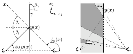
Figure 2: Graphical representation of a reflection off edge $\gamma$. On the left, the law of reflection prescribes $\theta_{r}=\theta_{i}$. We show the straight line $\widetilde{\gamma}$ supporting $\gamma$ with a dotted stroke. For a given observation point $\bm{x}$, $\bm{y}(\bm{x})$ denotes the point of incidence of the reflected field component. On the right, computation of the spatial support $\Omega_{n}$ (light-grey area) and its complementary shadow zone $\Omega\setminus\Omega_{n}$ (dark-grey area) for the reflected field component, in the presence of a rectangular obstacle. The dashed portion of edge $\gamma$ denotes the shadow $\gamma\setminus\gamma^{(i)}$. The shadow zone consists of two connected components.

Weight function $\zeta_{n}$

Let $\bm{x}-\bm{\xi}_{n}$ be a generic point where we wish to evaluate the weight function $\zeta_{n}$. We define the incidence point $\bm{y}(\bm{x})$ as the intersection (if any) between edge $\gamma$ and the segment from $\bm{\xi}_{n}$ to $\bm{x}$. See Fig. 2 (left). According to the method of images, the amplitude of the reflected wave is equal (up to sign) to the amplitude of the incoming wave:

$$\zeta_{n}(\bm{x}-\bm{\xi}_{n})=\pm\zeta_{i}(\bm{y}(\bm{x})-\bm{\xi}_{i}).$$ (12)

Above and throughout this section, the sign $\pm$ depends on the type of boundary conditions on the edge $\gamma$ (“$+$” for Neumann, “$-$” for Dirichlet).

Now, recall that we are assuming all weight functions $\zeta_{i}$ to be positive-homogeneous. According to Remark 2.2, this means that $\zeta_{i}(\bm{x}-\bm{\xi}_{i})$ is only a function of the angle $\phi_{i}(\bm{x})$ between $\bm{x}-\bm{\xi}_{i}$ and the positive $x_{1}$-axis. See Fig. 2 (left) for a graphical depiction. Specifically, with an abuse of notation, let $\zeta_{i}(\bm{x}-\bm{\xi}_{i})=\zeta_{i}(\phi_{i}(\bm{x}))$ and $\zeta_{n}(\bm{x}-\bm{\xi}_{n})=\zeta_{n}(\phi_{n}(\bm{x}))$, where the “new” angle-dependent functions $\zeta_{i}$ and $\zeta_{n}$ are $2\pi$-periodic. By Eq. 12, we deduce the property

$$\zeta_{n}(\phi_{n}(\bm{x}))=\pm\zeta_{i}(\phi_{i}(\bm{y}(\bm{x})))= \pm\zeta_{i}(2\beta_{\gamma}-\phi_{n}(\bm{y}(\bm{x})))$$

$$= \pm\zeta_{i}(2\beta_{\gamma}-\phi_{n}(\bm{x})),$$ (13)

where $\beta_{\gamma}$ is the angle between edge $\gamma$ and the positive $x_{1}$-axis. This uniquely identifies $\zeta_{n}$, given $\zeta_{i}$ and $\beta_{\gamma}$.

Spatial support $\Omega_{n}$

We first identify what portion of $\gamma$ is actually “lit” by $\widetilde{u}_{i}$: $\gamma^{(i)}=\gamma\cap\overline{\Omega_{i}}$. Note that we may have $\gamma\neq\gamma^{(i)}$, for instance when obstacles are present between $\bm{\xi}_{i}$ and $\gamma$. See Fig. 2 (right) for an illustration. Then, roughly speaking, we define the new support $\Omega_{n}$ as the union of all line segments from $\bm{\xi}_{n}$ that pass through $\gamma^{(i)}$. To be more precise, given $\bm{x}\in\Omega$, let $\bm{y}(\bm{x})$ be the intersection (if any) between $\gamma$ and the line segment from $\bm{\xi}_{n}$ to $\bm{x}$. Also, if $\bm{y}(\bm{x})$ exists, we define $\tau_{0}(\bm{x})=\left\|\bm{y}(\bm{x})-\bm{\xi}_{n}\right\|/\left\|\bm{x}-\bm{\xi}_{n}\right\|\in(0,1)$, which satisfies $\bm{y}(\bm{x})=\bm{\xi}_{n}+\tau_{0}(\bm{x})(\bm{x}-\bm{\xi}_{n})$. The new support is defined as

$$\Omega_{n}=\left\{\bm{x}\in\Omega\ :\ \bm{y}(\bm{x})\in\gamma^{(i)}\text{ and }\bm{\xi}_{n}+\tau(\bm{x}-\bm{\xi}_{n})\in\Omega\ \ \forall\tau_{0}(\bm{x})<\tau\leq 1\right\}.$$ (14)

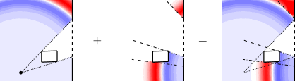
Figure 3: Example of reflection off an edge in the presence of an obstacle, from Fig. 2. Neumann conditions are imposed on all edges. Source wave (left), reflected wave (middle), and superimposition of the two (right). Note how the obstacle creates a shadow zone for source and reflected waves. For simplicity, in this plot we are not showing any reflection or diffraction effects due to the rectangular obstacle, since they would be modeled at different stages of the algorithm.

Figure 3 represents a possible output of the numerical algorithm. In this case, we simulate only the reflections, thus discarding, for the time being, any effect due to diffraction. It is clear that, by modeling reflection effects only, we may obtain a discontinuous approximation of the solution of our target problem, with discontinuities arising at the boundaries of the spatial supports identified so far. As we will see in the next section, introducing diffraction in our approximation will allow us to obtain a continuous approximation $\widetilde{u}$.

4 Modeling diffraction

Here, we describe a strategy for modeling waves diffracted by a vertex of the domain boundary $\partial\Omega$. This is required in building a new field component $\widetilde{u}_{n}$ whenever the smallest unexplored entry of the timetable is related to a vertex, i.e., $j>n_{e}$ in Algorithm 1, cf. Section 2.

In our modeling, we take inspiration from the uniform theory of diffraction (UTD) [19, 17]. UTD provides an effective description of diffraction in the frequency domain, which we need to specialize for our time-domain modeling. This task is difficult for several reasons. On the one hand, standard approaches for frequency-to-time-domain conversion involve the inversion of the Fourier transform, which is rather costly in a numerical setting, where integration/convolution must be replaced by quadrature. (This issue actually affects also time-domain diffraction modeling based on impulse responses, see, e.g., [20, 21].) On the other hand, UTD is an asymptotic method, whose accuracy relies on assuming the frequency to be sufficiently large. As such, an inverse Fourier transform is not guaranteed to provide sound results, whenever the signal bandwidth includes low frequencies.

Both these reasons behoove us to develop a novel time-domain version of UTD. Specifically, we wish our diffraction modeling to fit in the framework of Eq. 5, so that:

• Diffraction is modeled as a wave outgoing from a point source at some $\bm{\xi}_{n}$. This is actually in line with standard approaches, e.g., [22, 5], where diffraction is modeled through virtual sources on the vertex (in 2D) or edge (in 3D) that causes the diffraction event. This motivates the choice of the center $\bm{\xi}_{n}:=\bm{y}_{j^{\prime}}=\bm{y}_{j-n_{e}}$, the diffraction vertex (we are employing the notation of Algorithm 1).

• Diffraction has a spatial support $\Omega_{n}$, which (again in accordance to diffraction theory) we define as the set of all points that are visible (along straight-line paths) from $\bm{\xi}_{n}$, i.e.,

  $$\Omega_{n}=\left\{\bm{x}\in\Omega\ :\ \bm{\xi}_{n}+\tau(\bm{x}-\bm{\xi}_{n})\in\Omega\ \ \forall 0<\tau\leq 1\right\}.$$ (15)

• The space-time dependence of the diffraction amplitude should be separable into an angular component $\zeta_{n}$, and a radial-temporal component, which, in fact, is assumed to coincide with the free-space wave propagation profile $\Psi$.

The last step is the most critical one, and we devote the remainder of the present section to it.

From a phenomenological point of view, the angular modulation $\zeta_{n}$ can be related to the diffraction coefficient appearing in geometrical diffraction theory [16, 19]. Indeed, the diffraction coefficient $D$ has exactly the desired role of scaling factor for the diffraction amplitude, which depends on the angle that the target measurement point $\bm{x}$ forms with the edges adjacent the diffraction vertex. In 2-dimensional UTD, the diffraction coefficient depends on the above-mentioned angle between $\bm{x}$ and $\bm{\xi}_{n}$, but also on (i) the domain geometry locally around the diffraction point, (ii) the location of the source that causes the diffraction, (iii) the frequency of the incident signal, and (iv) the distance $\left\|\bm{x}-\bm{\xi}_{n}\right\|$. The UTD expression of $D$ is provided in Appendix A.

The last two above-mentioned items are problematic in our framework: since we work in the time domain, we do not have a single incident frequency $k$; moreover, due to our separability assumption, we require the angular modulation to be independent of $\left\|\bm{x}-\bm{\xi}_{n}\right\|$. However, frequency and radial distance always appear together, as a product, in the UTD diffraction coefficient. Specifically, such product $\mu:=k\left\|\bm{x}-\bm{\xi}_{n}\right\|$ can be interpreted as the distance between $\bm{x}$ and the diffraction point $\bm{\xi}_{n}$, measured in wavelength units.

In practice, the value of $\mu$ determines how quickly the magnitude of $D$ decays to $0$, as one moves away from a so-called “shadow boundary”, i.e., the boundary of the spatial support of either the incident or the reflected wave(s). Equivalently, $\mu$ determines the width of the transition region, which encompasses any shadow boundaries. See Appendices A and 13. Also, note that UTD requires $\mu$ to be large enough ($\geq 1$), and that $\mu\to\infty$ yields the geometrical-optics setting, i.e., a diffraction-free model, with $\zeta_{n}\equiv 0$.

Since the dependence of $D$ on the two troublesome terms happens only through $\mu$, we propose the following strategy for defining a $k$- and $\left\|\bm{x}-\bm{\xi}_{n}\right\|$-independent angular modulation $\zeta_{n}$: we set $\zeta_{n}$ as the diffraction coefficient $D$ obtained for some value of $\mu=\overline{\mu}$ that is fixed a priori. Such value $\overline{\mu}$ should be sufficiently large not to cause issues in UTD, but also sufficiently small to avoid the geometrical-optics pitfall.

Obviously, the specific choice of $\overline{\mu}$ should be based on the ultimate approximation target: minimizing the discrepancy between $u$ and $\widetilde{u}$. However, it turns out that $D$ depends relatively mildly on the value of $\mu$. See Appendix A for a theoretical justification, and Section 5.1 for some numerical tests. In our experiments, we settle for the value $\overline{\mu}=10$. A more careful quantitative investigation of the role of $\mu$ on the diffraction approximation accuracy is envisioned as a future research direction.

Remark 4.1.

Instead of using frequency-domain UTD, the time-domain diffraction coefficient could be computed by convolution of the incoming wave with a “diffraction impulse response”, as done in [21, 23]. Such a convolution would need to be approximated (by quadrature) over and over, at each diffraction event. Notably, since the diffraction impulse response is not a Dirac delta, a convolution with it naturally introduces a radial modulation too. This entails that the diffraction wave does not behave like an angular modulation of the free-space wave $\Psi$, as assumed in our model.

Our modeling of diffraction through a diffraction coefficient that does not depend on time nor radius, although biased in the above-described way, is very efficient, as it avoids the expensive computation of convolutions with the diffraction impulse response. As we will show in our numerical experiments, this increased efficiency comes at the cost of a relatively small modeling error. As such, our approach remains justified.

5 Numerical results

In our experiments, we require a “reference” solution of Eq. 1 to validate our results. To this effect, we use the solution $u_{\textup{FE}}$ obtained by discretizing Eq. 1 with:

• the P1-finite element (FE) method with mass-lumping, over a regular triangulation (mesh) of the physical domain $\Omega$;

• explicit leapfrog timestepping with a uniform time step that satisfies the CFL condition on the chosen mesh.

See [7, 8] for more details on this discretization strategy.

If the domain $\Omega$ is unbounded, we first need to truncate it in such a way that reflections from the non-physical truncation boundary do not affect the solution in the region of interest for $t<T$. Recalling that the problem data are supported in a ball of radius $R$ and center $\bm{0}$, this can be done, e.g., by truncating $\Omega$ at the sphere with radius $R+T$ (we recall that we are assuming a unit wave speed) and center $\bm{0}$. In our tests, we rely on FEniCS [24] to carry out the FE discretization on 2-dimensional domains $\Omega$. Note that, instead, unbounded geometries are allowed in our proposed approach, making domain truncations unnecessary.

All our tests are performed in Python 3.8 on a machine with an 8-core 4.70 GHz Intel^® processor. For reproducibility, our code is made available at https://github.com/pradovera/ray-wave-2d.

5.1 Some simple wedges

As a way to assess our proposed method in simple settings, we consider four different “wedge” domains. We define $\Omega$ to be one of the portions of the plane $\mathbb{R}^{2}$ delimited by two straight lines intersecting at a point, with $\alpha$ being the outer angle at such point. The specific choices of wedge angles $\alpha$ are reported in Table 1 for the four cases.

Example	exterior	incidence	$\left\|\widetilde{u}(\cdot,T)\right\|_{L^{2}(\Omega)}$	$\left\|\widetilde{u}(\cdot,T)-u_{\textup{FE}}(\cdot,T)\right\|_{L^{2}(\Omega)}$
index	angle $\alpha$	angle $\theta$
#1	$4.712$	$0.984$	$2.50\cdot 10^{-1}$	$3.65\cdot 10^{-4}$
#2	$5.093$	$0.603$		$2.07\cdot 10^{-3}$
#3	$2.761$	$1.363$		$7.84\cdot 10^{-3}$
#4	$2.761$	$3.277$		$1.17\cdot 10^{-2}$

Table 1: Setup for the four wedge examples. The angle $\theta$ is as in Fig. 4.

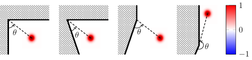
Figure 4: Initial conditions for the wedge examples, indexed #1 through #4 from left to right. The (dashed) distance between the center of the Gaussian and the boundary vertex is 4 units in all cases.

We set up a wave-propagation problem like Eq. 1, with $u_{0}$ an isotropic Gaussian with standard deviation $0.2$. The center of $u_{0}$ is at a point located at a 4-unit distance from the wedge vertex, in the direction determined by the “incidence angle” $\theta$. See Fig. 4 for a representation of the initial conditions in the four cases. We set $u_{1}=f=0$, we enforce Neumann boundary conditions on the whole $\partial\Omega$, and we seek the solution at the final time $T=5$, i.e., $1$ time unit after the wave crest has reached the wedge vertex.

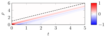
Figure 5: Free-space solution $\Psi$. The dashed line denotes the upper bound of the “causality cone” of $\Psi$, i.e., $\rho=t+R$, with $R=1$.

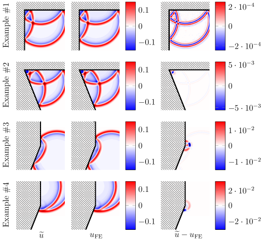
Figure 6: Results for the four wedge examples. Each row pertains to a different example. In each row, from left to right: surrogate solution, FE solution, and error. The color scales for the first two columns are the same. All results are shown at the final time $t=T$.

To this aim, we employ our proposed approach, see Section 2. First, we compute an approximation of the free-space solution $\Psi$, which solves Eq. 4, by employing the P1-FE method with explicit leapfrog timestepping. Note that, since Eq. 4 is cast in polar coordinates, we only need to discretize a 1D interval with P1-FE. Since the initial condition $u_{0}$ is supported within the unit disk, we have $R=1$, and it suffices to approximate $\Psi(\rho,t)$ for $(\rho,t)\in[0,T+R]\times[0,T]$. Since this space-time domain is only 2-dimensional, we can afford a very fine discretization. In our experiments, we employ a $1001\times 2001$ uniform Cartesian space-time grid, i.e., the mesh size is $\delta x=\frac{T+R}{1000}$ and the time step is $\delta t=\frac{T}{2000}$. This satisfies the CFL condition. We show the resulting $\Psi$ (which, in fact, we should denote by $\Psi_{\textup{FE}}$) in Fig. 5. Note that, since we are solving the wave equation in 2D, the magnitude of $\Psi$ decays like $\mathcal{O}(t^{-1/2})$ as $t\to\infty$, which corresponds to a spatial decay of $\mathcal{O}(\rho^{-1/2})$. In 3D, the decay would be quicker, namely, $\mathcal{O}(t^{-1})$ in time and $\mathcal{O}(\rho^{-1})$ in space.

After this preliminary step, we use the timetable-based strategy from Section 2 to identify reflection and scattering effects, which are then added up to give the final approximation $\widetilde{u}$. We show the resulting $\widetilde{u}(\cdot,T)$ in Fig. 6. In this figure, we also display a reference solution $u_{\textup{FE}}(\cdot,T)$, which we obtain by direct discretization of Eq. 1 by P1-FE and leapfrog timestepping, as described at the beginning of Section 5.

In all four examples, we see that $\widetilde{u}$ and $u_{\textup{FE}}$ seem qualitatively close. Notably, we can observe a good representation of the most prominent wavefronts, which are due to propagation of either the main “free-space” wave or to its reflections. Indeed, those wave contributions are reconstructed exactly: the only errors are the ones due to FE approximation and timestepping, which affect both $u_{\textup{FE}}$ and $\widetilde{u}$ (the latter through the approximation of $\Psi$). Instead, some differences are present when comparing diffraction effects, which arise as circular waves about the wedge vertex. We can quantitatively observe this in the last column of both Tables 1 and 6.

In example #1, we observe a very small error, which, in fact, is simply the (FE and timestepping) discretization error. This is related to the fact that the wedge index $\nu=\pi/(2\pi-\alpha)=2$ is an integer, thus making diffraction unnecessary in approximating the wave $u$ [17].

In the other examples, diffraction effects are necessary to correctly identify $u$. While a good qualitative behavior can be observed in Fig. 6, we can see in Table 1 that a modest error is present. Specifically, we report the $L^{2}(\Omega)$-norm of $\widetilde{u}$ and of the error $\widetilde{u}-u_{\textup{FE}}$ at the final time $t=T$, defined as

$$\left\|v\right\|_{L^{2}(\Omega)}=\left(\int_{\Omega}v(\bm{x})^{2}\textup{d}\bm{x}\right)^{1/2}.$$ (16)

We see the largest error in example #4, where the relative $L^{2}(\Omega)$-approximation error amounts to about $5\%$. This example corresponds to a case of “almost grazing” incidence, with the source point being located rather close to one of the wedge’s edges. In turn, this leads to two shadow boundaries located very close to each other, with overlapping transition regions, cf. Appendix A. We interpret this result as evidence of the fact that our diffraction model from Section 4 is less accurate with grazing than with non-grazing incidence. Despite this, the error remains small in all the above tests, and our diffraction model may be considered satisfactory overall.

5.1.1 Building a cavity out of wedges

As a slightly more complicated example, we now combine the four wedges from the previous section to obtain the open cavity represented in Fig. 7. In this case, more reflection and diffraction effects arise, due to the trapping nature of the domain. Our initial conditions and forcing term are the same as before, but now all edges are sound-soft. Accordingly, we model them using Dirichlet boundary conditions. The time horizon is $T=9$.

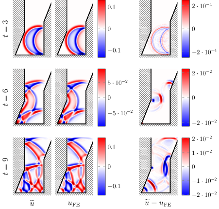
Figure 7: Results for the cavity domain. Each row corresponds to a different time instant $t\in\{3,6,9\}$, from top to bottom. In each row, from left to right: surrogate solution $\widetilde{u}(\cdot,t)$, FE solution $u_{\textup{FE}}(\cdot,t)$, and error $\widetilde{u}(\cdot,t)-u_{\textup{FE}}(\cdot,t)$. The color scales for the first two columns are the same.

Using our strategy from Section 2, we build the approximation $\widetilde{u}$, which contains $45$ wave terms ($1$ source wave, $32$ reflected waves, and $12$ diffraction waves). We compare the approximation $\widetilde{u}$ with the reference solution $u_{\textup{FE}}$, obtained as described at the beginning of Section 5, on a mesh with around $10^{6}$ degrees of freedom.

We show the results of the comparison in Fig. 7, at 3 time instants $t\in\{3,6,9\}$. Once more, we see a good qualitative agreement between $\widetilde{u}$ and $u_{\textup{FE}}$, with the most important features of $u$ being identified well. We see “error waves” of small amplitude propagating from the 3 vertices of $\Omega$ that generate diffraction effects. These correspond to errors in diffraction modeling.

The approximation $\widetilde{u}$ is built in approximately $500$ms, out of which $420$ms are used to compute the free space solution $\Psi$. This is a surprisingly small time, compared to the computation of the reference $u_{\textup{FE}}$, which takes about a minute, with the 2D meshing alone taking around $20$s.

As an additional experiment to validate our diffraction modeling, we study how the approximation error depends on the choice of $\overline{\mu}$, which we use to compute the diffraction coefficient, as described in Section 4. We compute the $L^{2}(\Omega)$-approximation error at times $t=6$ and $t=9$, for values of $\overline{\mu}$ between $1$ and $100$. Note that every value of $\overline{\mu}$ involves the computation of a new diffraction coefficient $D$ for each diffraction event, but otherwise does not require retraining the surrogate: only the angular weights $\zeta_{n}$ may vary.

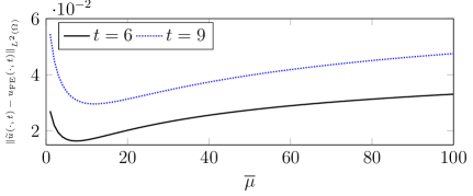
Figure 8: $L^{2}(\Omega)$-approximation error at $t=6$ and $t=9$ for different values of $\overline{\mu}$.

In Fig. 8, we show how the errors have a minimum around $\overline{\mu}=7$ for $t=6$, and around $\overline{\mu}=11$ for $t=9$. This shift in the minimum point seems to suggest that larger values of $\overline{\mu}$ should be used for approximations at longer times, an observation that may be especially relevant for simulations over long time horizons. That being said, the error appears to vary only mildly around the locations of such minima: for instance, at $t=6$, the error obtained for $\overline{\mu}=10$ is $1.68\cdot 10^{-2}$, only $2\%$ more than the minimum error $1.64\cdot 10^{-2}$. (Note also the narrowness of the vertical scale of the plot.) This provides an empirical justification for choosing a single value of $\overline{\mu}$ (around $10$) for all diffraction events, and for all times $t$.

5.2 A tall room

We now move to a simplified sound propagation problem in a room. For simplicity, we consider a 2-dimensional problem, thus assuming an infinitely tall room, and modeling line sources (in the $z$-direction) as point sources.

The complicated domain $\Omega\subset\mathbb{R}^{2}$ is depicted in Fig. 9. It is composed of two communicating “rooms” with sound-hard walls, as well as of a third large room (above), which is modeled as infinitely large. In the main room, three sound-soft triangular obstacles are also present.

Setting once more $u_{1}=f=0$, we are interested in modeling the propagation of an initial condition $u_{0}$ modeled as a Ricker wavelet centered at $\bm{0}$, see Fig. 9 (top left), over the time horizon $t\in[0,T]$, with $T=20$. To this aim, we employ our proposed method from Section 2.

As in the previous example, we start by computing an approximation of the free-space solution $\Psi=\Psi(\rho,t)$ for $(\rho,t)\in[0,T+R]\times[0,T]$, see Eq. 4, with $R$ being the radius of the support of the initial condition $u_{0}$. Again, we use P1-FE with leapfrog timestepping for this.

Since many reflective surfaces face each other, the domain $\Omega$ is trapping. Accordingly, we expect the number $N$ of waves in the approximation $\widetilde{u}$ to be rather large. In the interest of reducing the number of such terms, we employ the on-the-fly tolerance-based strategy described in Remark 2.3, removing all wave terms $\widetilde{u}_{n}$ whose magnitude is smaller than $\textup{tol}=2.5\cdot 10^{-2}$. After this, $N=798$ terms are left. Although this value of $N$ may seem large, the evaluation of the corresponding surrogate $\widetilde{u}$ is rather quick, due to the explicit nature of each wave contribution (and to the fact that their supports are smaller than the whole $\Omega$).

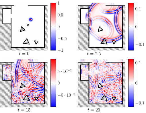
Figure 9: 2-dimensional domain $\Omega$ modeling a room. Top left plot: initial condition $\widetilde{u}(\cdot,0)=u(\cdot,0)=u_{0}$, a Ricker wavelet; we also show the point $\bm{x}_{\textup{trace}}$ as a cross. Top right plot: intermediate solution $\widetilde{u}(\cdot,7.5)$. Bottom left plot: intermediate solution $\widetilde{u}(\cdot,15)$. Bottom right plot: final solution $\widetilde{u}(\cdot,20)$.

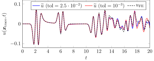
Figure 10: Value of solution at point $\bm{x}_{\textup{trace}}=(-1,-2)$.

We show the resulting $\widetilde{u}(\cdot,t)$ for the four times $t\in\{0,7.5,15,20\}$ in Fig. 9. There, we can see why so many terms are necessary for the approximation of $u$: we must model many reflection and diffraction effects. Since energy escapes the system only through the top “door”, the wave will persist for quite a long time. Accordingly, a larger $T$ will make a larger $N$ necessary.

In order to better inspect this effect, we show the trace of the solution at the arbitrarily chosen point $\bm{x}_{\textup{trace}}=(-1,-2)$ in Fig. 10. We notice that oscillations persist for $t>10$. We use this last plot also to validate our results. To this aim, we compare:

• The surrogate $\widetilde{u}$ obtained as described above, with $\textup{tol}=2.5\cdot 10^{-2}$.

• The surrogate $\widetilde{u}$ obtained with our strategy, but with $\textup{tol}=10^{-3}$. This leads to an increased number of rays $N\approx 9.7\cdot 10^{3}$.

• The reference solution $u_{\textup{FE}}$ obtained by the P1-FE with leapfrog timestepping, as described at the beginning of Section 5. The mesh size must be chosen small enough to resolve both the initial condition and the domain $\Omega$ well. In our case, we have a mesh with approximately $1.4\cdot 10^{6}$ elements. To satisfy the CFL condition on this mesh, we choose a time step $\Delta t\approx 7\cdot 10^{-3}$.

We can observe that the two surrogates obtained with our approach give very similar results. Indeed, the cutoff tolerance tol affects the results only for sufficiently large $t$, due to the accumulation of “small” waves that are excluded from the coarser surrogate but included in the finer one.

Moreover, taking the FE solution as reference, we see that most of the peaks of the surrogates are aligned with the FE ones (i.e., the “phase” of the wave is well approximated), but there are some noticeable discrepancies in their amplitudes. This is due to the fact that, in our approach, reflection is modeled exactly, whereas the magnitudes of the diffraction waves are only approximated. For this reason, we should not expect the amplitude error to get smaller if we reduce tol. The only effective way of improving the approximation would be using a more accurate diffraction model.

As a final result, we also report:

• The “construction” time, i.e., the time required to compute the numerical solution. For $\widetilde{u}$, this means executing Algorithm 1. For $u_{\textup{FE}}$, this means building the mesh, assembling the FE stiffness and (lumped) mass matrices, and carrying out the timestepping.

• The “evaluation” time, i.e., the time required to evaluate the numerical solution ($\widetilde{u}$ or $u_{\textup{FE}}$) at a single $(\bm{x},t)$-point.

They can be found in Table 2.

	$\widetilde{u}$ ($\textup{tol}=2.5\cdot 10^{-2}$)	$\widetilde{u}$ ($\textup{tol}=10^{-3}$)	$u_{\textup{FE}}$
Construction [s]	$10.29$	$138.8$	$92.14$
Evaluation [$\mu$s]	$338$	$4710$	$38.9$

Table 2: Timings for the room test case. To obtain more statistically significant results, each displayed time is the average over $3$ (resp. $10^{3}$) runs of the construction (resp. evaluation) phase with identical parameters.

We can observe the increased construction and evaluation times that result from decreasing tol. Moreover, we see that, in this example, our proposed approach is more competitive in the construction phase, but less so in the evaluation phase. The larger evaluation time of our surrogate is ultimately due to the nonlinearity of the functions that appear in $\widetilde{u}$. In this context, it may be surprising to note that, in our implementation, the most expensive step in evaluating $\widetilde{u}$ (taking about half of the online time) is determining whether an evaluation point is in the spatial supports $\Omega_{n}$ or not.

On the other hand, evaluating the FE solution at a space-time point is an extremely cheap operation, essentially corresponding to a vector dot product. However, the FE solution comes with the serious drawback of memory usage. Indeed, in our example, storing $u_{\textup{FE}}$ as a $(\sim 1.5\cdot 10^{6})\times(\sim 2.9\cdot 10^{3})$ array of double-precision floating-point numbers requires approximately $34$ GB. For more complex domains or, e.g., for 3D problems, storing such a matrix in RAM might simply be unfeasible. In particular, we note that storing the whole “timestepping history” is a necessity if one wishes to access point-evaluations of $u_{\textup{FE}}$ at arbitrary times after the timestepping has been carried out.

5.2.1 A time-harmonic source

One of the advantages of our approach is that it allows changing the source terms of the problem in a seamless way. Notably, under minor technical constraints (e.g., the spatial support of the new source term should not be larger than the old one), this kind of change does not require training a new surrogate.

To showcase this, we approximate the wave propagating from a time-harmonic point source at $\bm{x}=\bm{0}$ with angular frequency $\omega>0$. In our tests, we pick $\omega\in\{2\pi,10\pi\}$. To this aim, we define $u$ as the solution of the following ($\omega$-dependent) problem:

$$\begin{cases}\partial_{tt}u(\bm{x},t)=\Delta u(\bm{x},t)-\omega^{2}\sin(\omega t)\delta_{\bm{0}}(\bm{x})\quad&\text{for }(\bm{x},t)\in\Omega\times(0,T),\\ u(\bm{x},0)=0\quad&\text{for }\bm{x}\in\Omega,\\ \partial_{t}u(\bm{x},0)=0\quad&\text{for }\bm{x}\in\Omega,\\ \partial_{\nu}u(\bm{x},t)=0\quad&\text{for }(\bm{x},t)\in\partial\Omega\times(0,T],\end{cases}$$ (17)

where $\delta_{\bm{0}}$ denotes the 2-dimensional Dirac delta.

As usual, we define $\Psi=\Psi(\rho,t)$ as the ($\omega$-dependent) solution of the free-space version of Eq. 17 in radial-temporal coordinates. The free-space solution $\Psi$ has space-time support $\{(\rho,t)\in[0,\infty)^{2},\rho\leq t\}$, which is a subset of the free-space solution from the previous section, namely, $\{(\rho,t)\in[0,\infty)^{2},\rho\leq t+R\}$. As such, to obtain an approximation for the wave $u$ generated by the time-harmonic source for an arbitrary $\omega$, it suffices to plug the corresponding $\Psi$ in each term of the surrogate $\widetilde{u}$ from the previous section! We show the results of our approximation in Fig. 11, where we can observe a good agreement between approximation and reference FE solution. Similarly to the previous examples, inaccuracies become more prominent for larger times, where more and more contributions are removed from the surrogate model as a consequence of the truncation tolerance tol.

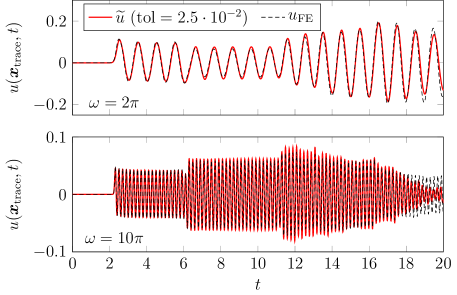
Figure 11: Value of solution at point $\bm{x}_{\textup{trace}}=(-1,-2)$ for excitation frequencies $\omega=2\pi$ (top) and $\omega=10\pi$ (bottom). The reference FE solution is also included in both plots as a dashed line.

Note that using FE to approximate the wave $u$ requires carrying out a new simulation from scratch for every frequency to be studied. To this end, one needs to choose a mesh with $\omega$-dependent resolution: the mesh size should be small enough for the well-known pollution effect (see, e.g., [25]) to be absent.

A constraint on the mesh resolution is present also in our proposed approach. However, it only applies to the problem defining the free-space solution $\Psi$, which is 1-dimensional in space. Hence, having to refine the mesh represents a much smaller obstacle to efficiency. In particular, as the frequency $\omega$ increases, the computation of $\widetilde{u}$ becomes comparatively more and more efficient, with respect to the computation of $u_{\textup{FE}}$.

6 Conclusions

We have presented a surrogate modeling strategy for approximating waves propagating through complex 2-dimensional domains with polygonal boundaries. Our method relies on the automatic identification of reflection and diffraction effects caused by the domain geometry. Each effect is modeled through a relatively simple nonlinear expression. Reflection-related components are built using geometrical optics, whereas diffraction-related components are modeled by a novel ad hoc modification of the geometrical theory of diffraction.

In our numerical tests, we have observed a good accuracy, with the main features of the target wave being well identified. Notably, our diffraction model has proven to be fairly effective. Still, it relies on the parameter $\mu$, which, in some sense, determines the strength of surrogate diffraction effects. Although we have presented some heuristics for choosing $\mu$, more refined strategies for selecting $\mu$ and, more generally, a thorough validation of our diffraction model remain open issues.

In terms of complexity, our method requires the solution of a simplified 1D-in-space problem, much simpler than the original 2D-in-space one. We expect such advantage to be even more relevant if one were to consider 3D instead of 2D problems.

Another favorable aspect of our algorithm is its potential to be run on parallel architectures, since the computation of different rays can be carried out independently. This is not the case for standard timestepping-based discretizations, due to their intrinsically sequential nature.

Finally, we recall that, in many applications, the ultimate target is understanding how the wave $u$ solving Eq. 1 depends on underlying parameters $\mathbf{p}$, e.g., the forcing term $f$, the shape of the domain $\Omega$, etc. In this setting, MOR algorithm try to construct a surrogate model of the form $\widetilde{u}=\widetilde{u}(\bm{x},t;\mathbf{p})$, providing a good approximation of $u$ over a whole range of parameter values. Even though our technique was presented here in the non-parametric setting, we believe that it potentially allows incorporating the parameter dependence in a natural and efficient way. In our opinion, this might be achievable by leveraging the simple and interpretable structure of the field components (free-space solution, spatial support, and angular modulation). As a simple preliminary example, we showcased this in Section 5.2.1 for a parametric source term, with the parameter being the frequency. We are currently investigating how to extend our method to more complicated parametric problems.

Appendix A UTD diffraction coefficient

Consider the setup shown in Fig. 12: a wedge with exterior angle $\alpha$ and vertex $\bm{\xi}_{n}$ is hit by a wave coming from $\bm{\xi}$, located at an angular position $\phi=\theta$. The angle $\phi$ is measured from one of the two sides of the wedge.

Let $\bm{x}$ be a point located at distance $s=\left\|\bm{x}-\bm{\xi}_{n}\right\|$ from $\bm{\xi}_{n}$, at an angle $\phi=\phi(\bm{x})$. The diffraction coefficient $D=D(\bm{x})$ represents the magnitude (and sign) of the diffraction wave at $\bm{x}$, assuming that the incident wave, with origin at $\bm{\xi}$, is time-harmonic with unit amplitude and frequency $k$. UTD [17] predicts a diffraction coefficient

$$D=D_{1}+D_{2}\pm(D_{3}+D_{4}),$$

with the sign $\pm$ depending on the type of boundary conditions (“$+$” for Neumann, “$-$” for Dirichlet). Given the wedge index $\nu:=\pi/(2\pi-\alpha)$, all contributions $D_{j}$ have the form

$$D_{j}=-\frac{\nu}{2\sqrt{2\pi ks}}\cot(\widehat{\phi}_{j})F\left(2ks\cos(\widetilde{\phi}_{j})^{2}\right),$$

with

$$\widehat{\phi}_{1}=\frac{\pi+\phi-\theta}{2}\nu,\quad\widetilde{\phi}_{1}= N_{1}(2\pi-\alpha)-\frac{\phi-\theta}{2},$$

$$\widehat{\phi}_{2}=\frac{\pi-\phi+\theta}{2}\nu,\quad\widetilde{\phi}_{2}= N_{2}(2\pi-\alpha)-\frac{\phi-\theta}{2},$$

$$\widehat{\phi}_{3}=\frac{\pi+\phi+\theta}{2}\nu,\quad\widetilde{\phi}_{3}= N_{3}(2\pi-\alpha)-\frac{\phi+\theta}{2},$$

$$\widehat{\phi}_{4}=\frac{\pi-\phi-\theta}{2}\nu,\quad\widetilde{\phi}_{4}= N_{4}(2\pi-\alpha)-\frac{\phi+\theta}{2},$$

and

$$F(x)=2\sqrt{x}\sqrt{\left(\int_{\sqrt{x}}^{\infty}\cos(y^{2})\textrm{d}y\right)^{2}+\left(\int_{\sqrt{x}}^{\infty}\sin(y^{2})\textrm{d}y\right)^{2}}.$$

The integers $N_{j}$ are defined as

$$N_{1}=\left[\frac{\nu}{2}\right],\quad N_{2}=\left[-\frac{\nu}{2}\right],\quad N_{3}=\left[\frac{1+\nu}{2}\right],\quad\text{and}\quad N_{4}=\left[\frac{1-\nu}{2}\right],$$

with square brackets denoting the rounding operator, which yields the integer that is closest to its argument.

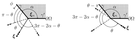
Figure 12: Diagrams for the two cases of scattering for concave corners ($0<\alpha<\pi$): without (left plot) and with shadow zone (right plot). The dashed lines are reflection boundaries. The dash-dotted line is a shadow boundary. Shadow regions are absent if and only if $\pi-\alpha\leq\theta\leq\pi$. The angular coordinate $0<\phi<2\pi-\alpha$ is measured starting from one of the two adjacent edges of $\partial\Omega$.

The diffraction coefficient has unit jumps (with suitable signs) at the shadow boundaries, i.e., at the angular positions corresponding to boundaries of the spatial support of the source wave (in which case, we have an “incident shadow boundary”, ISB) or of one of its reflections (in which case, we have a “reflection shadow boundary”, RSB). The locations of the shadow boundaries can be identified geometrically. For instance, for convex wedges ($0<\alpha<\pi$), shadow boundaries are at $\phi=\left|\pi-\theta\right|$ (which is an ISB if $\theta>\pi$, and an RSB otherwise) and at $\phi=2\pi-\alpha-\left|\pi-\alpha-\theta\right|$ (which is an ISB if $\theta<\pi-\alpha$, and an RSB otherwise).

The diffraction coefficient for $\alpha=\frac{\pi}{3}$, $\theta=\frac{\pi}{5}$, Neumann conditions, and $ks\in\{1,10,100\}$ are shown in Fig. 13 (left). Two jumps happen, at an RSB (at $\phi=\frac{4}{5}\pi$) and at an ISB (at $\phi=\frac{6}{5}\pi$). Similar results are obtained for Dirichlet conditions, cf. Fig. 13 (right).

We can observe that the value of $ks$ determines how quickly $D$ decays to 0 around each shadow boundaries: larger values of $ks$ yield a narrower “transition region”, which, loosely speaking, is the support of $D$ around each discontinuity. Indeed, asymptotically in $ks$, the width of each transition region is proportional to $1/\sqrt{ks}$ [19].

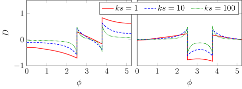
Figure 13: UTD diffraction coefficients for Neumann (left) and Dirichlet (right) wedges.

References

- [1] L. Borcea, V. Druskin, A. V. Mamonov, M. Zaslavsky, Robust nonlinear processing of active array data in inverse scattering via truncated reduced order models, Journal of Computational Physics 381 (2019) 1–26. doi:10.1016/j.jcp.2018.12.021.
- [2] L. Borcea, V. Druskin, A. V. Mamonov, M. Zaslavsky, J. Zimmerling, Reduced order model approach to inverse scattering, SIAM Journal on Imaging Sciences 13 (2) (2020) 685–723. doi:10.1137/19M1296355.
- [3] L. Borcea, G. Papanicolaou, C. Tsogka, J. Berryman, Imaging and time reversal in random media, Inverse Problems 18 (5) (2002). doi:10.1088/0266-5611/18/5/303.
- [4] P. H. Tournier, I. Aliferis, M. Bonazzoli, M. de Buhan, M. Darbas, V. Dolean, F. Hecht, P. Jolivet, I. El Kanfoud, C. Migliaccio, F. Nataf, C. Pichot, S. Semenov, Microwave tomographic imaging of cerebrovascular accidents by using high-performance computing, Parallel Computing 85 (2019) 88–97. doi:10.1016/j.parco.2019.02.004.
- [5] L. Savioja, U. P. Svensson, Overview of geometrical room acoustic modeling techniques, The Journal of the Acoustical Society of America 138 (2) (2015) 708–730. doi:10.1121/1.4926438.
- [6] S. F. Potter, M. K. Cameron, R. Duraiswami, Numerical geometric acoustics: An eikonal-based approach for modeling sound propagation in 3D environments, Journal of Computational Physics 486 (2023) Article 112111. doi:https://doi.org/10.1016/j.jcp.2023.112111.
- [7] G. Cohen, A. Hauck, M. Kaltenbacher, T. Otsuru, Different Types of Finite Elements, in: S. Marburg, B. Nolte (Eds.), Computational Acoustics of Noise Propagation in Fluids - Finite and Boundary Element Methods, Springer Berlin Heidelberg, Berlin, Heidelberg, 2008, pp. 57–88. doi:10.1007/978-3-540-77448-8_3.
- [8] E. Hairer, G. Wanner, C. Lubich, Geometric Numerical Integration, Vol. 31 of Springer Series in Computational Mathematics, Springer Berlin Heidelberg, Berlin, Heidelberg, 2002. doi:10.1007/978-3-662-05018-7.
- [9] P. Benner, M. Ohlberger, A. Cohen, K. Willcox, Model reduction and approximation: theory and algorithms, SIAM, 2017. doi:10.1137/1.9781611974829.
- [10] S. Glas, A. T. Patera, K. Urban, A reduced basis method for the wave equation, International Journal of Computational Fluid Dynamics 34 (2) (2020) 139–146. doi:10.1080/10618562.2019.1686486.
- [11] J. S. Hesthaven, C. Pagliantini, G. Rozza, Reduced basis methods for time-dependent problems, Acta Numerica 31 (2022) 265–345. doi:10.1017/S0962492922000058.
- [12] C. Greif, K. Urban, Decay of the Kolmogorov N-width for wave problems, Applied Mathematics Letters 96 (2019) 216–222. doi:10.1016/j.aml.2019.05.013.
- [13] N. Cagniart, Y. Maday, B. Stamm, Model Order Reduction for Problems with Large Convection Effects, in: Contributions to Partial Differential Equations and Applications, Vol. 47, Springer International Publishing, Cham, 2019, pp. 131–150. doi:10.1007/978-3-319-78325-3_10.
- [14] H. Kleikamp, M. Ohlberger, S. Rave, Nonlinear model order reduction using diffeomorphic transformations of a space-time domain, in: MATHMOD 2022 Discussion Contribution Volume, ARGESIM Publisher Vienna, 2022, pp. 57–58. doi:10.11128/arep.17.a17129.
- [15] J. Reiss, P. Schulze, J. Sesterhenn, V. Mehrmann, The shifted proper orthogonal decomposition: A mode decomposition for multiple transport phenomena, SIAM Journal on Scientific Computing 40 (3) (2018) A1322–A1344. doi:10.1137/17M1140571.
- [16] J. B. Keller, Geometrical theory of diffraction, J. Opt. Soc. Am. 52 (2) (1962) 116–130. doi:10.1364/JOSA.52.000116.
- [17] R. G. Kouyoumjian, P. H. Pathak, A uniform geometrical theory of diffraction for an edge in a perfectly conducting surface, Proceedings of the IEEE 62 (11) (1974) 1448–1461. doi:10.1109/PROC.1974.9651.
- [18] H. Lee, B.-H. Lee, An efficient algorithm for the image model technique, Applied Acoustics 24 (2) (1988) 87–115. doi:10.1016/0003-682X(88)90033-3.
- [19] D. A. McNamara, C. W. I. Pistorius, J. A. G. Malherbe, Introduction to the uniform geometrical theory of diffraction, Artech House Norwood, MA, 1990.
- [20] P. T. Calamia, U. P. Svensson, Fast time-domain edge-diffraction calculations for interactive acoustic simulations, EURASIP Journal on Advances in Signal Processing 2007 (2006) 1–10.
- [21] U. P. Svensson, R. I. Fred, J. Vanderkooy, An analytic secondary source model of edge diffraction impulse responses, The Journal of the Acoustical Society of America 106 (5) (1999) 2331–2344. doi:10.1121/1.428071.
- [22] M. A. Biot, I. Tolstoy, Formulation of wave propagation in infinite media by normal coordinates with an application to diffraction, The Journal of the Acoustical Society of America 29 (3) (2005) 381–391. doi:10.1121/1.1908899.
-
[23]
R. R. Torres, U. P. Svensson, M. Kleiner,
Computation of edge diffraction for
more accurate room acoustics auralization, The Journal of the Acoustical
Society of America 109 (2) (2001) 600–610.
doi:10.1121/1.1340647.
URL https://doi.org/10.1121/1.1340647 - [24] M. S. Alnæs, J. Blechta, J. Hake, Others, The FEniCS Project version 1.5, Archive of Numerical Software 3 (100) (2015).
- [25] I. M. Babuška, S. A. Sauter, Is the pollution effect of the fem avoidable for the helmholtz equation considering high wave numbers?, SIAM Journal on Numerical Analysis 34 (6) (1997) 2392–2423. doi:10.1137/S0036142994269186.