Non-Singular Bouncing Model in Energy Momentum Squared Gravity

Abstract

This work is concerned to study the bouncing nature of the universe for an isotropic configuration of fluid $\mathcal{T}_{\alpha\beta}$ and Friedmann-Lemaître-Robertson-Walker metric scheme. This work is carried out under the novel $f(\mathcal{G},\mathcal{T}_{\alpha\beta}\mathcal{T}^{\alpha\beta})$ gravitation by assuming a specific model i.e, $f(\mathcal{G},\mathcal{T}^{2})=\mathcal{G}+\alpha\mathcal{G}^{2}+2\lambda\mathcal{T}^{2}$ with $\alpha$ and $\lambda$ are constants, serving as free parameters. The terms $\mathcal{G}$ and $\mathcal{T}^{2}$ served as an Gauss-Bonnet invariant and square of the energy-momentum trace term as an inclusion in the gravitational action respectively, and is proportional to $\mathcal{T}^{2}=\mathcal{T}_{\alpha\beta}\mathcal{T}^{\alpha\beta}$. A specific functional form of the Hubble parameter is taken to provide the evolution of cosmographic parameters. A well known equation of state parameter, $\omega(t)=-\frac{k\log(t+\epsilon)}{t}-1$ is used to represent the dynamical behavior of energy density, matter pressure and energy conditions. A detailed graphical analysis is also provided to review the bounce. Furthermore, all free parameters are set in a way, to make the supposed Hubble parameter act as the bouncing solution and ensure the viability of energy conditions. Conclusively, all necessary conditions for a bouncing model are checked.

Keywords: cosmography; Hubble Parameter; $f(\mathcal{G},\mathcal{T}_{\alpha\beta}\mathcal{T}^{\alpha\beta})$.
PACS: 98.80.-k; 04.20.Cv; 04.50.Kd.

1 Introduction

According to the big bang hypothesis, the whole universe was created by a single explosion, with all matter in the cosmos as an infinite speck [1, 2]. This hypothesis works well in order to study the beginning, but lack to define different cosmological problems. These problems include the horizon problem, the flatness problem, the singularity problem, etc. In order to resolve these big cosmic challenges, different cosmic theories have been developed in literature [3, 4, 5]. The bouncing hypothesis is one of the major independent theories that came up with the answers related to the starting of the universe and should be enough to resolve the major cosmic problem of singularity. The bouncing cosmology works on the scheme of an oscillatory universe, i.e, a universe that came into being from the pre-existing universe without undergoing the singularity [6, 7, 8]. This whole transition of the universe not only explains the big-bang cosmology but also reduces one of the major issues. For the bouncing, the universe moves into the contraction phase as a matter-dominated the era of the universe. After the contraction, the universe starts to expand in a nonsingular manner for which gravity dominates the matter [9, 10]. Also, density perturbations can be produced during the bounce era. This idea of the origination of the universe is highly accepted and appreciated in literature.

General relativity ($\mathcal{GR}$) was presented by Einstein and it was thought to be one of the best theories to explain different cosmological issues. It explains the gravity under the fabric of space-time. However, to understand gravity much more effectively and to provide the answers to the effect of gravity, dark energy, and accelerated expansion of the universe under the addition of different scalar fields, different attempts have been made in past to modify $\mathcal{GR}$. These modifications change the geometric or matter or both parts of the Einstein field equations accordingly. These could help to discuss the effects of couplings of matter and curvature terms on the above-described items. Roshan and Shojai [11] presented the nonlinear form of matter term i.e, $\mathcal{T}^{2}=\mathcal{T}_{\alpha\beta}\mathcal{T}^{\alpha\beta}$, naming it $f(\mathcal{R},\mathcal{T^{2}})$. They further indicated that the use of nonlinear terms may provide the prevention of early time singularities. Since the functional form of curvature terms has helped to introduce new gravitational theories, so it was considered to be effective to modify the generic action integral of $\mathcal{GR}$ as corrections. These modifications give light to the $f(\mathcal{G})$ theory, for which the term $\mathcal{G}$ is defined as $\mathcal{G}=\mathcal{R}_{\xi\zeta\alpha\beta}\mathcal{R}^{\xi\zeta\alpha\beta}-4\mathcal{R}_{\xi\zeta}\mathcal{R}^{\xi\zeta}+\mathcal{R}^{2}$. Nojiri and Odintsov [12] introduced this $f(\mathcal{G})$ theory for the first time in their work. They tested solar systems for this formalism and reported the phase change of acceleration to deceleration for the achievement of phantom line, which cooperated to study dark energy. Odintsov and Oikonomou [13] considered $\mathcal{R}+f(\mathcal{G})$ form of the gravitational theory to provide their contribution to the study of gravitational baryogenesis. Their work included the higher-order derivatives of Gauss-Bonnet terms that work in order to produce the baryon asymmetry. Sharif and Ikram [14] gives rise to a new theory by following the footsteps of Harko. They coupled the matter part $\mathcal{T}$ with the geometric part of the $f(\mathcal{G})$ theory, making it $f(\mathcal{G},\mathcal{T})$ cosmology. They investigated the validity of their theory with the help of energy conditions. Later on, Bhatti et al.[15] worked on the $f(\mathcal{G},\mathcal{T})$ theory to carry out the investigation of some physically feasible features of compact star formation. They inferred that the compactness of a star model grows at the core whereas the energy conditions remain constant. Yousaf and his mates [16] inspired by [17], have recently developed a novel $f(\mathcal{G},\mathcal{T}^{2})$ to present the complexity of structural scalars from the use of Herrera’s method of splitting scalars. They considered the exponential coupling of Gauss-Bonnet terms as a functional form as $f(\mathcal{G},\mathcal{T}^{2})=\alpha\mathcal{G}^{n}(\beta\mathcal{G}^{m}+1)+\eta\mathcal{T}^{2}$, to explore the validity of their solutions for the Darmois and Israel conditions. They also worked on the non-static complex structures under the same theory to describe the effects of an electromagnetic field. They used specific model configuration i.e, $f(\mathcal{G},\mathcal{T}^{2})=k_{1}\mathcal{G}^{m}(k_{2}\mathcal{G}^{n}+1)+\lambda\mathcal{T}^{2}$, in their work.

Bouncing cosmology has gained much reputation over the past few years, because of its independent hypothetical nature from different standard comic problems. Guth [18] during $1980^{\prime}s$, had put forward his inflationary theory to tackle early and late time cosmic evolutionary problems. He remained successful in solving some related problems, but the answer to the initial singularity is still under concern. One of the best hypotheses to answer the singularity problem is the bouncing nature of the universe. The nature of the bouncing universe allows a certain universe model to transit from a pre-big crunch (contracted) phase into a new big bang (expanded) phase with the exclusion of singularity during the whole event [19]. Steinhardt and Ijjas [20] are considered to be the pioneers of the bouncing hypothesis. They devised a wedge diagram for a smooth bouncing method to explore the consequences of some cosmological problems. Sahoo et al. [21] worked on the non-singular bouncing by assuming the specific coupling of $\mathcal{R}$ and $\mathcal{T}$ as $f(\mathcal{R},\mathcal{T})=\mathcal{R}+\chi\mathcal{R}\mathcal{T}$, for $0<\chi<\frac{\pi}{4}$. They allowed such a parametric approach for the Hubble parameter to provide no singularity during the bounce. They used quintom and phantom scalar field configurations for the bouncing paradigm. Bamba and his collaborators [22] inspected the singularity-free concept of bounce by considering an exponential form of scale factor $a(t)=\sigma\exp(\lambda t)+\tau\exp(\lambda t)$ under the effect of $f(\mathcal{G})$ gravity. They checked the stability of their assumed solution under the restricted parametric scheme.

Yousaf et al. [23, 24] explored the bouncing universe with a specific functional form of Hubble parameter by taking exponential $f(\mathcal{G},\mathcal{T})$ form. Different cosmic models are under consideration for the scale factor in order to determine the value of expansion and contraction at the current cosmic phase and also to predict the current phase equation of state. These models predicted different results in the literature. However, cosmography provided us a benefit in processing cosmological data for explaining the universal kinematics without the involvement of the gravity model and hence provided that the cosmography can be employed with the Taylor expansions as an alternative scheme. Also, the cosmographic analysis for the $\mathcal{FLRW}$ universe, is helpful in such a way that it can put aside the effect of the dynamical field equations [25]. Gruber et al. [26] studied an alternative approach to describe cosmography by extending the conventional methodology. They resulted from numerical values of the cosmographic parameters by applying the $Pad\acute{e}$ approximations. The testing of the $\Lambda$CDM model had been conveyed by Busti et al. [27] with the use of cosmographical analysis. Capozziello et al. provided cosmography as a non-predictive phenomenon when the redshift parameter becomes $z\approx 1$. They used the pad$\acute{e}$ approximations for the fifth order and resulted the divergence of data at the higher levels of the approximations. Lobo et al. [28] evaluated the dynamics of the redshift drift. They used the expanding $FLRW$ universe to produce a general matter and low redshift model with the use of different variables. However, the cross-correlation of large-scale quasars can be used and translated with the CMB and BAO scale data to produce the best for Hubble parameter $H(z)$ and angular diametric distance $S_{A}$. Also, the cosmic chronometers approach can be done to predict the model independent $H(z)$ measurements which have been extensively used for cosmological applications [29, 30, 31]. The low redshift data set with the inclusion of the megamasers and chronometers had been presented by Krishnan and others [32]. They result that the Hubble constant $\mathcal{H}_{0}$, showed descending behavior with the redshift and having non-zero slop when fitted on the line by statistical means. Font et al. [33] studied correlation technique for quasars by using Lya absorption and produced the best line of fit for Planck’s data. They generated different results on the measurements of the Hubble parameter and the angular distance. One important thing is to develop such a cosmic Hubble parameter that comes from early to late span in such a way that it changes from a low to a high value. The Gaussian method helped to predict but provided a non-transitional behavior for both $\Lambda$ and $\omega$ epochs. The null energy condition also proved to be an important restriction for the cut-off model, when compared with Hubble parameter data [34]. King et al. [35] studied the future approximations of the redshift by the inclusion of dark energy. They tested the equation of state by the linear parametrization technique. Hu et al. [34] reported different values of the Hubble constant by the Gaussian method. Their research produced an effective reduction in the Hubble crisis and proposed the non-transitional behavior of the Hubble constant. Different dark energy models respective to holography and agegraphy had been conducted by Zhang et al. [36]. They produced different energy conditions for different red shift values and resulted in an effective role of energy conditions for different cosmic ages.

In this article, we implemented a functional form of the Hubble parameter that evolves periodically with cosmic time $t$ and investigate the bouncing nature of the universe in $f(\mathcal{G},\mathcal{T}_{\alpha\beta}\mathcal{T}^{\alpha\beta})$ gravity using a flat $\mathcal{FLRW}$ peacetime. This analysis of the bouncing universe involves one of the most important forms of $EoS$ parameter proposed in the literature [37, 38, 39]. The outline is given as: Sect.2 provides a brief introduction to $f(\mathcal{G},\mathcal{T}_{\alpha\beta}\mathcal{T}^{\alpha\beta})$ gravity with the necessary formalism of $\mathcal{FLRW}$ metric and modified field equations. Sect.3 builds the Hubble parameter as a bouncing solution for the produced field equations. The cosmographic parameters are also evaluated in this section. We provide the mathematical expressions of energy density and matter pressure for the assumed $EoS$ parameter form in Sect.4. The energy conditions are also formulated in the same fashion. Detailed graphical profiles of energy conditions are represented in the same section to discuss the evolution of the universe under the influence of restricted free parameters. Finally, the concluding remarks are made in Sect.5.

2 $f(\mathcal{G},\mathcal{T}_{\alpha\beta}\mathcal{T}^{\alpha\beta})$ Formalism

The modified action for the $f(\mathcal{G},\mathcal{T}_{\alpha\beta}\mathcal{T}^{\alpha\beta})$ gravity theory is defined as [16]

$$\mathbb{A}_{f(\mathcal{G},\mathcal{T}_{\alpha\beta}\mathcal{T}^{\alpha\beta})}=\frac{\sqrt{-g}}{2\kappa^{2}}\left(\int d^{4}x[f(\mathcal{G},\mathcal{T}_{\alpha\beta}\mathcal{T}^{\alpha\beta})+\mathcal{R}]+\int d^{4}x\mathcal{L}_{m}\right),$$ (1)

where $\mathcal{R}$ and $\mathcal{G}$ symbolize the Ricci scalar and the Gauss-Bonnet scalar terms, respectively and are provided as

$$\mathcal{R}\equiv g_{\alpha\beta}\mathcal{R}^{\alpha\beta},~{}~{}~{}~{}\mathcal{G}\equiv\mathcal{R}_{\xi\zeta\alpha\beta}\mathcal{R}^{\xi\zeta\alpha\beta}-4\mathcal{R}_{\xi\zeta}\mathcal{R}^{\xi\zeta}+\mathcal{R}^{2},$$ (2)

and $\kappa^{2}$ = $8\pi$G (G be the gravitational constant) and $\mathcal{L}_{m}=-p$. Also, the term $g$ implies the trace of the metric tensor $g_{\alpha\beta}$ with $T_{\alpha\beta}$, $R_{\xi\zeta\alpha\beta}$ and $R_{\alpha\beta}$ indicate the stress energy-momentum tensor, the Riemannian tensor, and the Ricci tensor respectively. The expression for $\mathcal{T}_{\alpha\beta}$ is given as

$$\mathcal{T}_{\alpha\beta}=\frac{-2}{\sqrt{-g}}\frac{\delta(\sqrt{-g}\mathcal{L}_{m})}{\delta g^{\alpha\beta}}.$$ (3)

Equation (3) yields the following expression, due the dependency of the matter Lagrangian $\mathcal{L}_{m}$ on $g_{\alpha\beta}$ components

$$\mathcal{T}_{\alpha\beta}=g_{\alpha\beta}\mathcal{L}_{m}-\frac{2\partial\mathcal{L}_{m}}{\partial g^{\alpha\beta}}.$$ (4)

Now, by taking the variation of Eq.(1) with respect to the term $g_{\alpha\beta}$, we get the following field equations for the $f(\mathcal{G},\mathcal{T}_{\alpha\beta}\mathcal{T}^{\alpha\beta})$ theory as

$$\mathcal{R}_{\alpha\beta}-\frac{1}{2}\mathcal{R}g_{\alpha\beta}=\mathcal{T}_{\alpha\beta}^{\emph{eff}},$$ (5)

where the term $\mathcal{T}_{\alpha\beta}^{\emph{eff}}$ takes the following form

$$\mathcal{T}_{\alpha\beta}^{\emph{eff}} = \kappa^{2}\mathcal{T}_{\alpha\beta}-\Theta_{\alpha\beta}f_{\mathcal{T}^{2}}(\mathcal{G},\mathcal{T}^{2})+\frac{1}{2}g_{\alpha\beta}f(\mathcal{G},\mathcal{T}^{2})-(2\mathcal{R}\mathcal{R}_{\alpha\beta}-4\mathcal{R}_{\alpha}^{\varepsilon}\mathcal{R}_{\varepsilon\beta}-4\mathcal{R}_{\alpha\varepsilon\beta\eta}\mathcal{R}^{\varepsilon\eta}$$ (6)

$$+2\mathcal{R}_{\alpha}^{\varepsilon\eta\delta}\mathcal{R}_{\beta\varepsilon\eta\delta})f_{\mathcal{G}}(\mathcal{G},\mathcal{T}^{2})-(2\mathcal{R}\nabla^{2}g_{\alpha\beta}-2\mathcal{R}\nabla_{\alpha}\nabla_{\beta}-4\mathcal{R}_{\alpha\beta}\nabla^{2}-4g_{\alpha\beta}\mathcal{R}^{\varepsilon\eta}\nabla_{\varepsilon}\nabla_{\eta}$$

$$+4\mathcal{R}^{\varepsilon}_{\alpha}\nabla_{\beta}\nabla_{\varepsilon}+4\nabla_{\varepsilon}\nabla_{\alpha}\mathcal{R}^{\varepsilon}_{\beta}+4\mathcal{R}_{\alpha\varepsilon\beta\eta}\nabla^{\varepsilon}\nabla^{\eta})f_{\mathcal{G}}(\mathcal{G},\mathcal{T}^{2}),$$

where,

$$\Theta_{\alpha\beta}\equiv\frac{\delta(\mathcal{T}_{\mu\nu}\mathcal{T}^{\mu\nu})}{\delta g^{\alpha\beta}}=2\mathcal{T}_{\alpha}^{\xi}\mathcal{T}_{\beta\xi}-\mathcal{T}\mathcal{T}_{\alpha\beta}-4\mathcal{T}^{\mu\nu}\frac{\partial^{2}\mathcal{L}_{m}}{\partial g^{\alpha\beta}g^{\mu\nu}}-2\mathcal{L}_{m}(\mathcal{T}_{\alpha\beta}-\frac{1}{2}\mathcal{T}g_{\alpha\beta})$$ (7)

$$\mathcal{T}^{2}=\mathcal{T}_{\alpha\beta}\mathcal{T}^{\alpha\beta},~{}~{}~{}~{}~{}\nabla^{2}=\nabla_{\alpha}\nabla^{\alpha}$$ (8)

The terms $f_{\mathcal{G}}(\mathcal{G},\mathcal{T}^{2})$ and $f_{\mathcal{T}^{2}}(\mathcal{G},\mathcal{T}^{2})$ used above are defined as

$$~{}~{}f_{\mathcal{G}}(\mathcal{G},\mathcal{T}^{2})\equiv\frac{df(\mathcal{G},\mathcal{T}^{2})}{d\mathcal{G}},~{}~{}~{}~{}and~{}~{}f_{\mathcal{T}^{2}}(\mathcal{G},\mathcal{T}^{2})\equiv\frac{df(\mathcal{G},\mathcal{T}^{2})}{d\mathcal{T}^{2}}.$$ (9)

The trace of the above-defined field equations is produced as

$$\mathcal{T}-\Theta f_{\mathcal{T}^{2}}(\mathcal{G},\mathcal{T}^{2})+2\mathcal{G}f_{\mathcal{G}}(\mathcal{G},\mathcal{T}^{2})-2\mathcal{R}\nabla^{2}f_{\mathcal{G}}(\mathcal{G},\mathcal{T}^{2})+4\mathcal{R}_{\alpha\beta}\nabla^{\alpha}\nabla^{\beta}f_{\mathcal{G}}(\mathcal{G},\mathcal{T}^{2})=0.$$ (10)

Equation (10) shows the non-conversed situation of the stress energy-momentum tensor. Also, the properties of $\mathcal{GR}$ can be recovered for $f(\mathcal{G},\mathcal{T}^{2})=0$. Similarly if we put $f(\mathcal{G},\mathcal{T}^{2})=f(\mathcal{G})$, we get the properties of $f(\mathcal{G})$ gravity.

Now, as we are concerned to study the bouncing nature of the universe, so we consider the fluid distribution to be perfect throughout the cosmic evolution. For this, we take

$$\mathcal{T}_{\alpha\beta}=(\rho+p)V_{\alpha}V_{\beta}-pg_{\alpha\beta},$$ (11)

here, the four-vector velocity is defined by $V^{\beta}$ with

$$V^{\beta}=(1,0,0,0),~{}~{}V^{\beta}V_{\beta}=1~{},~{}V^{\beta}\nabla_{\zeta}V_{\zeta}=0.$$ (12)

In addition, $\rho$ defines the energy density part and $p$ defines the pressure part of the stress energy-momentum tensor. Also the geometric background considered to be in a $\mathcal{FLRW}$ space time[40], so it implies

$$ds^{2}=dt^{2}-a^{2}(t)\Sigma_{i}dx_{i}^{2},~{}~{}~{}~{}~{}~{}~{}~{}~{}~{}~{}i=1,2,3.$$ (13)

The metric component $a(t)$ symbolizes the scale factor, that contributes to the Hubble parameter as $\mathcal{H}=\frac{\dot{a}(t)}{a(t)}$. Using Eq.(13) and Eq.(7) in Eq.(5), we get the following field equations

$$6\left(\frac{\dot{a}}{a}\right)^{2}-24\left(\frac{\dot{a}}{a}\right)^{3}\dot{f_{\mathcal{G}}}+24\left(\frac{\ddot{a}}{a}\right)\left(\frac{\dot{a}}{a}\right)^{2}f_{\mathcal{G}}-f-2(\rho^{2}+3p^{2}+4\rho p)f_{\mathcal{T}^{2}}=2\rho\kappa^{2},$$ (14)

$$-2\left(2\frac{\ddot{a}}{a}+\left(\frac{\dot{a}}{a}\right)^{2}\right)+16\left(\frac{\ddot{a}\dot{a}}{a^{2}}\right)\dot{f_{G}}+8\left(\frac{\dot{a}}{a}\right)^{2}\ddot{f_{G}}-24\left(\frac{\ddot{a}}{a}\right)\left(\frac{\dot{a}}{a}\right)^{2}f_{G}+f=2p\kappa^{2}.$$ (15)

To draw the conclusions on the field equations, we just need some functional form of $f(\mathcal{G},\mathcal{T}^{2})$. As, there are many functional forms regarding the interaction of matter with the curvature terms, in order to deal with the issues of cosmic evolution. Various coupling models can be used to evaluate the formations of both energy density and matter pressure, like one can take $f(\mathcal{G},\mathcal{T}^{2})=\mathcal{G}+2f(\mathcal{T}^{2})$ that may help to provide an analysis about $\Lambda CDM$ epoch. However, the other choice is $f(\mathcal{G},\mathcal{T}^{2})=f_{1}(\mathcal{G})+f_{2}(\mathcal{T}^{2})$ that may be worked as a correction to $f(\mathcal{G})$ gravity theory because of $f_{2}(\mathcal{T}^{2})$. Similar forms have been explored in [41, 42] and provided some distinct results due to the direct minimal curvature matter coupling. Also, $f(\mathcal{G},\mathcal{T}^{2})=f_{1}(\mathcal{G})+f_{2}(\mathcal{G})f_{3}(\mathcal{T}^{2})$ can be taken because of an explicit non-minimally coupling nature between geometric parameters and matter variables [43]. So, we considered the following form to produce the validating results.

$$f(\mathcal{G},\mathcal{T}^{2})=f_{1}(\mathcal{G})+f_{2}(\mathcal{T}^{2}).$$ (16)

To produce a bouncing universe, we need some functional forms of $f_{1}$ and $f_{2}$ that not only describe the accelerating expansion of the universe but also explain inflation to a great extent. For this, the higher power curvature terms perform well to eliminate such issues. Elizalde [44] introduced the power forms of the curvature scalar as $\eta\mathcal{R}^{n}$ ($n\geq 1$) and produced the cosmological dynamics, so we consider the specific form of the $f_{1}$ as the quadratic power model, so

$$f_{1}(\mathcal{G})=\mathcal{G}+\alpha\mathcal{G}^{2}.$$ (17)

Also, we take $\chi_{2}$ as

$$f_{2}(\mathcal{T}^{2})=2\lambda\mathcal{T}^{2}.$$ (18)

So, by using Eq.s (17) and (18) in the field equations, we get

$$6\mathcal{H}^{2}-48\alpha\mathcal{H}^{3}\mathcal{G}\dot{\mathcal{G}}+\alpha\mathcal{G}^{2}=2\kappa^{2}\rho+6\lambda\rho^{2}+18\lambda p^{2}+16\lambda\rho p,$$ (19)

and

$$-2(2\dot{\mathcal{H}}+3\mathcal{H}^{2})+32(\dot{\mathcal{\mathcal{H}}}+\mathcal{H}^{2})\alpha\mathcal{G}\dot{\mathcal{G}}+16\alpha\mathcal{H}^{2}(\dot{\mathcal{G}}^{2}+\mathcal{G}\ddot{\mathcal{G}})-\alpha\mathcal{G}^{2}=2\kappa^{2}p-2\lambda\rho^{2}-6\lambda p^{2}.$$ (20)

In order to reduce the complexity of the Eq.(19) and Eq.(20), we utilize $p=\omega\rho$, as the EoS used in [37, 38, 39]. So we get the relations,

$$(3\lambda+9\lambda\omega^{2}+8\lambda\omega)\rho^{2}+\kappa^{2}\rho-(3\mathcal{H}^{2}-24\alpha\mathcal{H}^{3}G\dot{\mathcal{G}}+\frac{\alpha}{2}\mathcal{G}^{2})=0$$ (21)

and

$$(-\frac{\lambda}{\omega^{2}}-3\lambda)p^{2}+\kappa^{2}p+((2\dot{\mathcal{H}}+3H^{2})-16(\dot{\mathcal{H}}+\mathcal{H}^{2})\alpha\mathcal{G}\dot{\mathcal{G}}-8\alpha\mathcal{H}^{2}(\dot{\mathcal{G}}^{2}+\mathcal{G}\ddot{\mathcal{G}})+\frac{\alpha}{2}\mathcal{G}^{2})=0.$$ (22)

where, $\mathcal{G}=24\mathcal{H}^{2}(\dot{\mathcal{H}}+\mathcal{H}^{2})$. Yousaf and his collaborators checked the stability of cosmic models in various modified gravity theories [45, 46, 47, 48].

3 Hubble Parameter and Cosmography

This section mainly focuses on describing the evolutionary behavior of these above-described dynamical terms. Hence, we consider a trigonometric form of the $\mathcal{H}(t)$ which feasibly provides a bounce solution [49, 44], as follows

$$\mathcal{H}(t)=\zeta\sin(\phi t)h(t).$$ (23)

This parameterized form of $\mathcal{H}(t)$ includes $\zeta$ and $\phi$, which are considered to be constants here. The choice of $h(t)$ depends on the periodic values of the function $\sin(\phi t)$, so the form of $h(t)$ can be chosen as periodic, that cooperates with the non-vanishing values of the above trigonometric function. This artificial approach of choosing such an ansatz can be considered as a numerical analysis of making the bouncing solution. One interesting feature is possessed by the term $\zeta$, which can work well as a phase changer for the value of $\mathcal{H}(t)$. We consider $h(t)$ as

$$h(t)=\exp(\varphi t),$$ (24)

where $\varphi$ acts as a constant. Finally, we have

$$\mathcal{H}(t)=\zeta\sin(\phi t)\exp(\varphi t).$$ (25)

This functional form of the Hubble parameter is helpful to study cosmic evolutionary expansion and contraction. This form of the Hubble parameter gives us the bounce at $t=313$, depending upon the values of $\varphi=0.001$ and $\phi=0.01$ provided in Fig.1. We have restricted the values of $\mathcal{H}(t)$ in the positive era of time. The basic scale factor form for this parameterized Hubble parameter becomes

$$a(t)=\exp\left(\frac{\zeta\exp(\varphi t)(\varphi\sin(\phi t)-\phi\sin(\phi t))}{\varphi^{2}+\phi^{2}}\right).$$ (26)

Similarly, the set of dynamical parameters that are derived from the Taylor series expansion of the scale factor is termed as cosmographic factors. These factors helped to obtain the cosmological concordance with the assumptions of the universal homogeneity and isotropy on large cosmic scales [27, 50]. These include deceleration, jerk and snap parameters. These factors allow us to check the compatibility of the scale factor and the Hubble parameter. The negative value of the deceleration parameter $q$ describes the accelerated expansion of the universe. Similarly, jerk $j$ and snap $s$ determine the expansion rate of the toy universe model. The mathematical interpretation for these cosmography elements are defined as

$$q=-\frac{1}{\mathcal{H}^{2}}\frac{1}{a}\frac{d^{2}a}{dt^{2}}=-1-\frac{1}{\zeta}(e^{-\varphi t}\csc(\phi t)(\phi\cot(\phi t)+\varphi)),$$ (27)

$$j=\frac{1}{\mathcal{H}^{3}}\frac{1}{a}\frac{d^{3}a}{dt^{3}} = 1+\frac{1}{\zeta^{2}}(e^{-2\varphi t}\csc(\phi t)(3\zeta e^{\varphi t}(\phi\cot(\phi t)+\varphi)$$ (28)

$$+\csc(\phi t)(2\varphi\phi\cot(\phi t)+\varphi^{2}-\phi^{2}))),$$

and

$$s=\frac{1}{\mathcal{H}^{4}}\frac{1}{a}\frac{d^{4}a}{dt^{4}}=-\frac{1}{3\zeta(3\zeta e^{\varphi t}+2\csc(\phi t)(\phi\cot(\phi t)+\varphi))}(2e^{-\varphi t}\csc(\phi t)(\csc(\phi t)$$

$$(3\zeta\varphi e^{\varphi t}\sin(\phi t)+\varphi^{2}-\phi^{2})+\phi\cot(\phi t)(3\zeta e^{\varphi t}+2\varphi\csc(\phi t)))).$$ (29)

Fig.1 shows the progression of the Hubble (left panel) and scale parameters (right panel) along the positive time axis. Similarly, the development of jerk (left panel) and snap factors (right panel) are provided in the fig.2. The evolution of the deceleration parameter towards the negative value i.e, $q\rightarrow-1$, before the bouncing point, provided in fig.6, shows the accelerating universe.

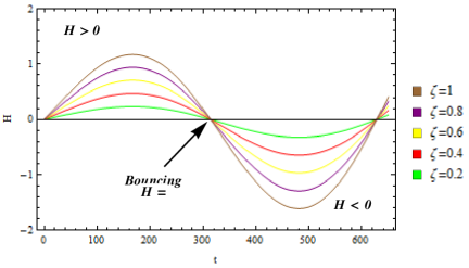
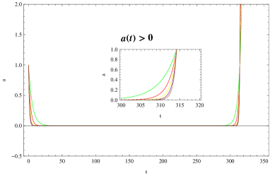
Figure 1: The illustrations of Hubble parameter and scale factor with fixed values of $\varphi=0.001$ and $\phi=0.01$.

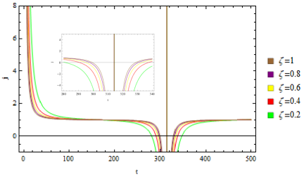
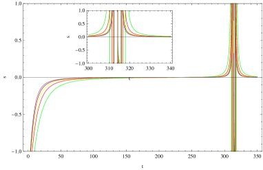
Figure 2: The illustration of jerk and snap factors with fixed values of $\varphi=0.001$ and $\phi=0.01$.

4 Energy Conditions under the EoS Parameter

For a specific cosmology model, energy conditions play an important role to make its validation for the restricted free parameters. These energy conditions help to maintain the specifications of the certain cosmic model [51, 52, 53, 54, 55]. Similarly, these energy conditions also work for the bouncing cosmology and provide a reasonable approach to validate the procedure for our toy bouncing model. These conditions are described as

• Dominant energy condition ($\mathcal{DEC}$)$\Leftrightarrow$ $\rho\geq 0$ , $\rho\pm p\geq 0$.

• Strong energy condition ($\mathcal{SEC}$)$\Leftrightarrow$ $\rho+3p\geq 0$ , $\rho+p\geq 0$.

• Weak energy condition ($\mathcal{WEC}$)$\Leftrightarrow$ $\rho\geq 0$ , $\rho+p\geq 0$.

• Null energy condition ($\mathcal{NEC}$)$\Leftrightarrow$ $\rho+p\geq 0$.

• Trace energy condition ($\mathcal{TEC}$)$\Leftrightarrow$ $\rho-3p\geq 0.$

The positivity of $\mathcal{DEC}$, $\mathcal{SEC}$ and $\mathcal{WEC}$ passes on the validity and necessity of the bouncing concept. However, the violation of $\mathcal{NEC}$ has a major role. This violation is different in the $\mathcal{GR}$ context. Universal bouncing scenario is one of those ideas that provides a chance to discuss the singularity-free universal beginning. Many proposals in the literature suggested avoiding this singularity through quantum aspects, but these don’t have such reliability to fit in the gravitational theory. So, at this point gravitational theories allow a specific mechanism to check the validity of the bounce model and as well its own. Null energy condition is one such tool to help achieve the task. Also, it has been proved that in the context of $\mathcal{GR}$, the violation of $\mathcal{NEC}$ is extremely difficult to be achieved for local-field models. So, effective field theories provide a chance to recognize the violation of the $\mathcal{NEC}$ and to allow a non-singular bounce [56, 57, 58, 59]. One such effective field is $f(\mathcal{G},\mathcal{T}_{\alpha\beta}\mathcal{T}^{\alpha\beta})$ theory that provides a chance to study the quadratic nature of the energy terms i.e, energy density and matter pressure[60, 16]. However, it also allows getting a non-singular bounce for the assumed gravity model form. For an excellent bouncing model, the value of $\mathcal{H}(t)$ turns out to be $\mathcal{\dot{H}}=-4G\rho\pi(1+\omega)>0$ for the formulation of $\mathcal{GR}$. However, if the $\mathcal{NEC}$ gets violated, we have the surety to get a bouncing scenario. To provide the mathematical formulation of the energy conditions, we consider Eqs. (21) and (22). Also, the $EoS$ parameter in the negative regime provides the present cosmic evolution [61, 62, 63] and becomes favorable in the bouncing context with $\omega(t)\approx-1$. However, bouncing cosmology provides the possible geodesic evolution of the universe by avoiding the singularity along with the resolution of the horizon problem, flatness problem, entropy problem and many more [5]. For the modified gravity, $EoS$ parameter enables us to study the universal dynamics. In this study, we used $EoS$ parameter [44] to obtain the possible chance of obtaining a bounce solution in $f(\mathcal{G},\mathcal{T}^{2})$ as

$$\omega(t)=-\frac{k\log(t+\epsilon)}{t}-1,$$ (30)

here $k$ is assumed to be a constant. This particular form of the $EoS$ parameters allows us to study the contracting and expanding behavior without involving the Hubble parameter as well as the scale factor. Elizalde et al. [44] produces cosmological dynamics by considering $\mathcal{R}^{2}$ gravity and logarithmic trace terms. They checked the effects of the $\lambda$ parameter in the gravity model $f(\mathcal{R},\mathcal{T})=\mathcal{R}+\lambda\mathcal{R}^{2}+2\beta\ln(\mathcal{T})$ along with the bouncing solution depending on the two $EOS$ parameters. Our work first described the choice of Hubble parameter and its effects on the dynamical field equations and then involves the $EOS$ parameter. We only took one of the $\omega(t)$ value, because this state factor after the bouncing point remains negative and becomes $\omega(t)\approx-1$. Also, the current cosmic expansion and $\Lambda-CDM$ can be verified by this state factor. However, the dynamic properties are greatly affected under the influence of this $EoS$ parameter form. Hence, the general forms of the Eqs.(21) and (22), under the influence of Eq.30, are presented as

$$\rho = -\frac{1}{2\lambda(9\omega^{2}+8\omega+3)}(\kappa^{2}+(\kappa^{4}-12\zeta^{2}\lambda(9\omega^{2}+8\omega+3)e^{2\varphi t}\sin^{2}(\phi t)(2304\alpha\zeta^{7}e^{7\varphi t}\sin^{4}(\phi t)$$ (31)

$$(\sin(\phi t)(\zeta e^{\varphi t}\sin(\phi t)+\varphi)+\phi\cos(\phi t))(4\zeta\varphi e^{\varphi t}\sin^{3}(\phi t)+2\zeta\phi e^{\varphi t}\sin(2\phi t)\sin(\phi t)$$

$$- (\phi^{2}-3\varphi^{2})\sin^{2}(\phi t)+2\phi^{2}\cos^{2}(\phi t)+3\varphi\phi\sin(2\phi t))-96\alpha\zeta^{4}e^{4\varphi t}\sin^{2}(\phi t)$$

$$(\sin(\phi t)(\zeta e^{\varphi t}\sin(\phi t)+\varphi)+\phi\cos(\phi t))^{2}-1))^{\frac{1}{2}}$$

$$p = \frac{1}{2(3\lambda\omega^{2}+\lambda)}(\kappa^{2}\omega^{2}+(\kappa^{4}\omega^{4}+4\zeta\omega^{2}(3\lambda\omega^{2}+\lambda)e^{\varphi t}(18432\alpha\zeta^{9}e^{9t\varphi}(2\varphi(2\varphi+1)-\phi^{2})$$ (32)

$$\sin^{10}(t\phi t)+4608\alpha\zeta^{8}e^{8t\varphi}(\varphi^{2}(25\varphi+22)-(13\varphi+2)\phi^{2})\sin^{9}(\phi t)+9216\alpha\zeta^{7}\phi^{3}e^{7\varphi t}$$

$$\sin^{5}(\phi t)\cos^{3}(\phi t)(7\zeta e^{\varphi t}\sin(\phi t)10\varphi+8)+288\alpha\zeta^{7}e^{7\varphi t}(144\varphi^{4}+320\varphi^{3}-16(9\varphi+4)$$

$$\varphi\phi^{2}-1)\sin^{8}(\phi t)+576\alpha\zeta^{6}\phi^{4}e^{6\varphi t}\sin^{4}(2\phi t)(\zeta e^{\varphi t}+2\csc(\phi t))+576\alpha\zeta^{6}\varphi e^{6\varphi t}$$

$$(48\varphi^{3}-16\varphi\phi^{2}-1)\sin^{7}(\phi t)-96\alpha\zeta^{5}\varphi(3\varphi-8)e^{5\varphi t}\sin^{6}(\phi t)+192\alpha\zeta^{4}e^{4\varphi t}(3\varphi^{2}-\phi^{2})$$

$$\sin^{5}(\phi t)+2\sin(\phi t)(5760\alpha\zeta^{6}\varphi\phi^{3}e^{6\varphi t}\sin^{3}(2\phi t)+48\alpha\zeta^{4}\phi^{2}e^{4\varphi t}\sin^{2}(2\phi t)-\varphi)+288\alpha$$

$$\zeta^{5}\phi^{2}e^{5\varphi t}\sin^{4}(\phi t)\cos^{2}(\phi t)(192\zeta^{4}e^{4\varphi t}\sin^{4}(\phi t)+32\zeta^{3}(31\varphi+10)e^{3\varphi t}\sin^{3}(\phi t)$$

$$+16\zeta^{2}e^{2\varphi t}(\varphi(45\varphi+56)-7\phi^{2})\sin^{2}(\phi t)+32\zeta e^{\varphi t}(17\varphi^{2}-\phi^{2})\sin(\phi t)-1)-2\phi\cos(\phi t)$$

$$(-18432\alpha\zeta^{9}(4\varphi+1)e^{9\varphi t}\sin^{9}(\phi t)-2304\alpha\zeta^{8}e^{8\varphi t}(\varphi(75\varphi+44)-11\phi^{2})\sin^{8}(\phi t)-9216\alpha\zeta^{7}$$

$$e^{7\varphi t}(3\varphi^{2}(3\varphi+5)-(4\varphi+1)\phi^{2})\sin^{7}(\phi t)-288\alpha\zeta^{6}e^{6\varphi t}(192\varphi^{3}-32\varphi\phi^{2}-1)$$

$$\sin^{6}(\phi t)+96\alpha\zeta^{5}(3\varphi-4)e^{5\varphi t}\sin^{5}(\phi t)-576\alpha\zeta^{4}\varphi e^{4\varphi t}\sin^{4}(\phi t)+1)$$

$$-3\zeta e^{\varphi t}\sin^{2}(\phi t)))^{\frac{1}{2}}$$

Now, the profiles of energy density and pressure under the presence of Eq.(30), are provided in fig.3. The plots indicate that the energy density suffers a positive behavior for the assumed values of free parameters. Similarly, the negative behavior for the pressure term indicates that the universe is in the accelerated expansion phase. However, the positive density proves a strong validation for the verification of the energy conditions. Also, one can get the positive and alternate trends of the both terms for different time periods due to the oscillatory behavior of the assumed Hubble parameter. We restrict our work for the positive density and negative pressure behavior to ascertain the energy conditions. The evolutionary profiles of the energy conditions are provided in the figs. 4 and 5. The $\mathcal{NEC}$ plot shows the violation with in the bouncing regime and confirms the major verification for the universe to attain a bounce with in the framework of $\mathcal{FLRW}$ spacetime. The violated $\mathcal{WEC}$ and $\mathcal{SEC}$ are given in the left plots of the figs. 3 and 4. The violated $\mathcal{SEC}$ also maintains the recent observations for the accelerating universe [52]. One important energy condition i.e, $\mathcal{TEC}$ has also been given in this recent study. The positive profiles for the $\mathcal{DEC}$ and $\mathcal{TEC}$ are given in the fig.5. The evolution of these energy conditions is strictly dependent on the values of the free parameters used in this study. However, one can get another configuration of these physical factors by implementing the different free parameters. The evolution of EoS parameter is provided in fig.6 to encounter the negative value i.e, $\omega(t)\approx-1$, for the current expansion phase of the universe.

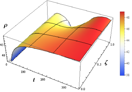
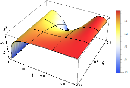
Figure 3: The illustration of energy density and matter pressure with fixed values of $\alpha=0.005$, $k=0.5$, $\varphi=0.001$, $\epsilon=0.001$, $\phi=0.01$, $\kappa=1$ and $\lambda=-0.005$.

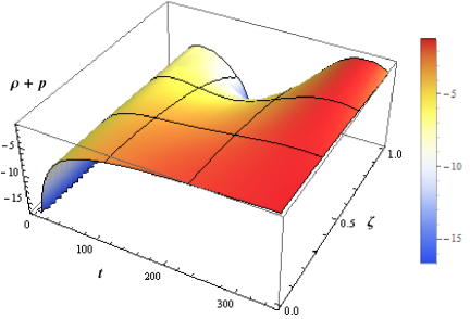
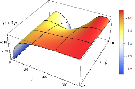
Figure 4: The illustration of $\mathcal{NEC}$ and $\mathcal{SEC}$ with fixed values of $\alpha=0.005$, $k=0.5$, $\varphi=0.001$, $\epsilon=0.001$, $\phi=0.01$, $\kappa=1$ and $\lambda=-0.005$.

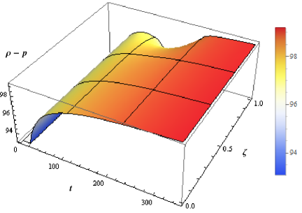
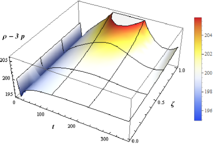
Figure 5: The illustration of $\mathcal{DEC}$ and $\mathcal{TEC}$ with fixed values of $\alpha=0.005$, $k=0.5$, $\varphi=0.001$, $\epsilon=0.001$, $\phi=0.01$, $\kappa=1$ and $\lambda=-0.005$.

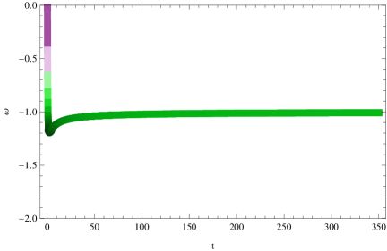
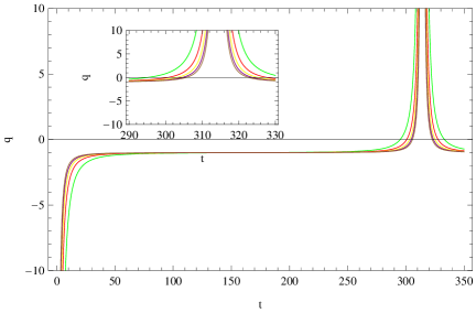
Figure 6: The illustration of EoS and deceleration parameters with fixed values of $k=0.5$ and $\epsilon=0.001$.

5 Discussions

This work involves the study of bouncing cosmology for an isotropic configuration of fluid $\mathcal{T}_{\alpha\beta}$ and $\mathcal{FLRW}$ metric. We comprehend this work under $f(\mathcal{G},\mathcal{T}_{\alpha\beta}\mathcal{T}^{\alpha\beta})$ theory of gravitation by assuming a specific model i.e, $f(\mathcal{G},\mathcal{T}^{2})=\mathcal{G}+\alpha\mathcal{G}^{2}+2\lambda\mathcal{T}^{2}$ with $\alpha$ and $\lambda$ are constants, serving as free parameters. This is the first-ever attempt to cover bouncing cosmology in the $f(\mathcal{G},\mathcal{T}_{\alpha\beta}\mathcal{T}^{\alpha\beta})$ theory. By the consideration of a specific functional form of the Hubble parameter, we discuss the evolution of cosmographic parameters. The assumption of a well-known equation of state (EoS) parameter, $\omega(t)=-\frac{k\log(t+\epsilon)}{t}-1$, is used as a direct implementation to represent the dynamical behavior of energy density, matter pressure, and energy conditions. The free parameters are restricted to the special values provided in each graph plot and are used for $\mathcal{H}(t)$ to act as the bouncing solution. The viability of energy conditions is studied with the help of a graphical approach. Following are the concluding remarks for this present work.

• The Hubble parameter $\mathcal{H}(t)$ used in this study is considered to have a trigonometric functional form. The evolutionary behavior of different cosmographic factors is described under the same form of $\mathcal{H}(t)$. This parameterized form of $\mathcal{H}(t)$ depends on the periodic values of the function $\sin(\phi t)$ and $h(t)$. We considered this $h(t)$ as a nonvanishing function for the periodic values of $\sin(\phi t)$. A perfect bouncing model allows the Hubble parameter to show the contraction phase i.e, $\mathcal{H}<0$, and when the universe expands it becomes $\mathcal{H}>0$. During this expansion and contraction phase, there is the point in between, at where $\mathcal{H}(t)$ becomes zero. So, in order to produce such a scenario, we have arranged the constants ($\phi$ and $\varphi$) in the Hubble parameter $(\mathcal{H}(t)=\zeta\sin(\phi t)\exp(\varphi t))$ to some specific values and notice the bounce at $t=313$. However, $t=313$ is significant in such a way that all the energy conditions necessary for the bounce, get satisfied accordingly till $t=313$, depending on the values of $\phi$ and $\varphi$. One can also produce other values of $t$ for bounce by restricting other values of $\phi$ and $\varphi$. The plot of $\mathcal{H}(t)$ is given in fig.1. The Hubble parameter gives us the bounce at $t=313$ which is the future singularity in the scale factor, see fig.1. The mathematical forms of deceleration, jerk, and snap are evaluated with the same $\mathcal{H}(t)$. The deceleration parameter tends to have a negative trend i.e, $q(t)$ approaches $-1$, which can be seen in fig.6. Similarly, the trends of jerk and snaps are given in fig.2 with $j(t)$ approaches to $1$ and $s(t)$ approaches to $0$. All these values show a deflection at the bouncing point, that fits in for the bouncing universe.

• We ensure the configuration of the bouncing cosmology by studying energy conditions. These energy conditions are provided in terms of energy density and matter pressure derived from the modified field equations. We assumed a specific EoS parameter in the form $\omega(t)=-\frac{k\log(t+\epsilon)}{t}-1$. This EoS parameter helped to maintain the positive and negative growth of energy density and matter pressure for the limited bouncing time period. The profiles of $\rho$ and $p$ are provided in the fig.3. However, the mathematical expression for these terms is evaluated in Eqs.(31) and (32).

• Under the restricted values of the free parameters, $\alpha=0.005$, $k=0.5$, $\varphi=0.001$, $\epsilon=0.001$, $\phi=0.01$, $\kappa=1$ and $\lambda=-0.005$, we get the violation of the $\mathcal{NEC}$ and $\mathcal{SEC}$. The violated $\mathcal{NEC}$ derives the bouncing nature of the universe. However, the violated $\mathcal{SEC}$ and $\mathcal{WEC}$ provide the phase of cosmic expansion. suitable with the observational data. The left plots of figs.3 and 4 shows the violated $\mathcal{SEC}$ and $\mathcal{WEC}$. Similarly, the positive behavior of $\mathcal{DEC}$ and $\mathcal{TEC}$ assure that the assumed model configuration is valid. Figure 5 represents the illustration of $\mathcal{DEC}$ and $\mathcal{TEC}$. Also, the evolution of EoS can be seen in fig.6, showing that $\omega(t)\rightarrow-1$. This value of $\omega(t)$ favors the current accelerated expansion phase of the universe [61, 62, 63].

• The above discussion provides that the bouncing evolution of the universe, studied in the framework of $f(\mathcal{G},\mathcal{T}^{2})=\mathcal{G}+\alpha\mathcal{G}^{2}+2\lambda\mathcal{T}^{2}$ and agrees with the recent astronomical observations [64, 65] i.e, all the energy conditions are fully satisfied, a great negative pressure behavior had been observed and provided help to study the late time accelerated universe [44]. However, this study can be used in the future for different models of the scale factors and Hubble parameters.

• We finally conclude that the bouncing evolution of the universe can be studied effectively with the oscillating nature of the scale factor under the flat $\mathcal{FLRW}$ regime.

References

- [1] C. J. Hogan, The little book of the big bang: A cosmic primer. Springer Science & Business Media, 1998.
- [2] A. H. Guth, “Eternal inflation,” Ann. N. Y. Acad. Sci., vol. 950, no. 1, pp. 66–82, 2001.
- [3] T. Padmanabhan and T. R. Seshadri, “Does inflation solve the horizon problem?,” Class. Quantum Gravity, vol. 5, no. 1, p. 221, 1988.
- [4] J. Earman and J. Mosterin, “A critical look at inflationary cosmology,” Philos. Sci., vol. 66, no. 1, pp. 1–49, 1999.
- [5] A. Ijjas and P. J. Steinhardt, “Bouncing cosmology made simple,” Class. Quantum Grav., vol. 35, no. 13, p. 135004, 2018.
- [6] E. Alesci, G. Botta, F. Cianfrani, and S. Liberati, “Cosmological singularity resolution from quantum gravity: The emergent-bouncing universe,” Phys. Rev. D, vol. 96, no. 4, p. 046008, 2017.
- [7] P. Das, S. Pan, S. Ghosh, and P. Pal, “Cosmological time crystal: Cyclic universe with a small cosmological constant in a toy model approach,” Phys. Rev. D, vol. 98, no. 2, p. 024004, 2018.
- [8] J. Mielczarek, M. Kamionka, A. Kurek, and M. Szydłowski, “Observational hints on the big bounce,” J. Cosmol. Astropart. Phys., vol. 2010, no. 07, p. 004, 2010.
- [9] Y.-F. Cai, R. Brandenberger, and P. Peter, “Anisotropy in a non-singular bounce,” Class. Quantum Gravity, vol. 30, no. 7, p. 075019, 2013.
- [10] Y.-F. Cai and X. Zhang, “Evolution of metric perturbations in a model of nonsingular inflationary cosmology,” J. Cosmol. Astropart., vol. 2009, no. 06, p. 003, 2009.
- [11] M. Roshan and F. Shojai, “Energy-momentum squared gravity,” Phys. Rev. D, vol. 94, no. 4, p. 044002, 2016.
- [12] S. Nojiri and S. D. Odintsov, “Modified Gauss–Bonnet theory as gravitational alternative for dark energy,” Phys. Lett. B, vol. 631, no. 1-2, pp. 1–6, 2005.
- [13] A. V. Astashenok, S. D. Odintsov, and V. K. Oikonomou, “Modified gauss–bonnet gravity with the lagrange multiplier constraint as mimetic theory,” Class. Quantum Gravity, vol. 32, no. 18, p. 185007, 2015.
- [14] M. Sharif and A. Ikram, “Energy conditions in f (G, T) gravity,” Eur. Phys. J. C ., vol. 76, no. 11, pp. 1–13, 2016.
- [15] M. Z. Bhatti, M. Y. Khlopov, Z. Yousaf, and S. Khan, “Electromagnetic field and complexity of relativistic fluids in f (G) gravity,” Mon. Not. Roy. Astron. Soc., vol. 506, pp. 4543–4560, 2021.
- [16] Z. Yousaf, M. Z. Bhatti, S. Khan, and P. K. Sahoo, “f theory and complex cosmological structures,” Phys. Dark Universe, p. 101015, 2022.
- [17] N. Katırcı and M. Kavuk, “ gravity and cardassian-like expansion as one of its consequences,” Eur. Phys. J. Plus, vol. 129, no. 8, pp. 1–12, 2014.
- [18] A. H. Guth, “Eternal inflation and its implications,” J. Phys. A, vol. 40, no. 25, p. 6811, 2007.
- [19] P. J. Steinhardt and N. Turok, “Cosmic evolution in a cyclic universe,” Phys. Rev. D, vol. 65, p. 126003, 2002.
- [20] A. Ijjas and P. J. Steinhardt, “Fully stable cosmological solutions with a non-singular classical bounce,” Phys. Lett. B, vol. 764, pp. 289–294, 2017.
- [21] S. Bhattacharjee and P. K. Sahoo, “Comprehensive analysis of a non-singular bounce in f (R, T) gravitation,” Phys. Dark Universe, vol. 28, p. 100537, 2020.
- [22] K. Bamba, A. N. Makarenko, A. N. Myagky, and S. D. Odintsov, “Bouncing cosmology in modified gauss–bonnet gravity,” Phys. Lett. B, vol. 732, pp. 349–355, 2014.
- [23] Z. Yousaf, M. Z. Bhatti, and H. Aman, “Cosmic bounce with T model,” Phys. Scr., vol. 97, no. 5, p. 055306, 2022.
- [24] Z. Yousaf, M. Z. Bhatti, and H. Aman, “The bouncing cosmic behavior with logarithmic law model,” Chin. J. Phys., vol. 79, pp. 275–286, 2022.
- [25] M. Visser, “Jerk, snap and the cosmological equation of state,” Class. Quantum Gravity, vol. 21, no. 11, p. 2603, 2004.
- [26] C. Gruber and O. Luongo, “Cosmographic analysis of the equation of state of the universe through padé approximations,” Phys. Rev. D, vol. 89, no. 10, p. 103506, 2014.
- [27] V. C. Busti, A. de la Cruz-Dombriz, P. K. Dunsby, and D. Saez-Gomez, “Is cosmography a useful tool for testing cosmology?,” Phys. Rev. D, vol. 92, no. 12, p. 123512, 2015.
- [28] F. S. N. Lobo, J. P. Mimoso, J. Santiago, and M. Visser, “Dynamical analysis of the redshift drift in f l r w universes,” 2022.
- [29] Moresco et al., “A 6% measurement of the hubble parameter at z 0.45: direct evidence of the epoch of cosmic re-acceleration,” J. Cosmol. Astropart. Phys., vol. 2016, no. 05, p. 014, 2016.
- [30] J. P. Hu, F. Y. Wang, and Z. G. Dai, “Measuring cosmological parameters with a luminosity-time correlation of gamma-ray bursts,” Mon. Not. Roy. Astron. Soc., vol. 507, no. 1, pp. 730–742, 2021.
- [31] F. Y. Wang, J. P. Hu, G. Q. Zhang, and Z. G. Dai, “Standardized long gamma-ray bursts as a cosmic distance indicator,” Astrophys. J., vol. 924, no. 2, p. 97, 2022.
- [32] Krishnan et al., “Is there an early universe solution to hubble tension?,” Phys. Rev. D, vol. 102, no. 10, p. 103525, 2020.
- [33] Font-Riberan et al., “Quasar-lyman forest cross-correlation from boss dr11: Baryon acoustic oscillations,” J. Cosmol. Astropart. Phys., vol. 2014, no. 05, p. 027, 2014.
- [34] J.-P. Hu and F.-Y. Wang, “Revealing the late-time transition of : relieve the hubble crisis,” Mon. Not. Royal Astron. Soc., vol. 517, no. 1, pp. 576–581, 2022.
- [35] A. L. King, T. M. Davis, K. D. Denney, M. Vestergaard, and D. Watson, “High-redshift standard candles: predicted cosmological constraints,” Mon. Not. Roy. Astron. Soc., vol. 441, no. 4, pp. 3454–3476, 2014.
- [36] M.-J. Zhang, C. Ma, Z.-S. Zhang, Z.-X. Zhai, and T.-J. Zhang, “Cosmological constraints on holographic dark energy models under the energy conditions,” Phys. Rev. D, vol. 88, no. 6, p. 063534, 2013.
- [37] E. Babichev, V. Dokuchaev, and Y. Eroshenko, “Dark energy cosmology with generalized linear equation of state,” Class. Quantum Grav., vol. 22, no. 1, p. 143, 2004.
- [38] J. Haro and E. Elizalde, “Gravitational particle production in bouncing cosmologies,” J. Cosmol. Astropart. Phys., vol. 2015, no. 10, p. 028, 2015.
- [39] A. P. Bacalhau, N. Pinto-Neto, and S. D. P. Vitenti, “Consistent scalar and tensor perturbation power spectra in single fluid matter bounce with dark energy era,” Phys. Rev. D, vol. 97, no. 8, p. 083517, 2018.
- [40] F. Melia, “The Friedmann–Lemaître–Robertson–Walker metric,” Mod. Phys. Lett. A, vol. 37, no. 03, p. 2250016, 2022.
- [41] Z. Yousaf, K. Bamba, and M. Z. Bhatti, “Causes of irregular energy density in gravity,” Phys. Rev. D, vol. 93, p. 124048, 2016.
- [42] M. F. Shamir, “Bouncing universe in f (G, T) gravity,” Phys. Dark Universe, vol. 32, p. 100794, 2021.
- [43] S. Nojiri, S. D. Odintsov, and V. K. Oikonomou, “Modified gravity theories on a nutshell: inflation, bounce and late-time evolution,” Phys. Rep., vol. 692, pp. 1–104, 2017.
- [44] E. Elizalde, N. Godani, and G. C. Samanta, “Cosmological dynamics in gravity with logarithmic trace term,” Phys. Dark Universe, vol. 30, p. 100618, 2020.
- [45] M. Sharif and Z. Yousaf, “Instability of meridional axial system in f(R) gravity,” Eur. Phys. J. C, vol. 75, p. 194, 2015.
- [46] M. Z. Bhatti, Z. Yousaf, and M. Ilyas, “Existence of wormhole solutions and energy conditions in f (R,T) gravity,” J. Astrophys. Astron., vol. 39, p. 69, 2018.
- [47] Z. Yousaf, “Definition of complexity factor for self-gravitating systems in Palatini f(R) gravity,” Phys. Scr., vol. 95, p. 075307, 2020.
- [48] M. M. M. Nasir, M. Z. Bhatti, and Z. Yousaf, “Influence of EMSG on complex systems: Spherically symmetric, static case,” Int. J. Mod. Phys. D, p. 10.1142/S0218271823500098.
- [49] M. F. Shamir, “Bouncing cosmology in gravity with logarithmic trace term,” Adv. Astron., vol. 2021, p. 8852581, 2021.
- [50] J. P. Hu and F. Y. Wang, “High-redshift cosmography: Application and comparison with different methods,” Astron. Astrophys., vol. 661, p. A71, 2022.
- [51] S. W. Hawking and G. F. R. Ellis, The large scale structure of space-time, vol. 1. Cambridge university press, 1973.
- [52] M. Visser, “Energy conditions in the epoch of galaxy formation,” Science, vol. 276, no. 5309, pp. 88–90, 1997.
- [53] S. Nojiri and S. D. Odintsov, “Effective equation of state and energy conditions in phantom/tachyon inflationary cosmology perturbed by quantum effects,” Phys. Lett. B, vol. 571, no. 1-2, pp. 1–10, 2003.
- [54] O. Bertolami and M. C. Sequeira, “Energy conditions and stability in f (R) theories of gravity with nonminimal coupling to matter,” Phys. Rev. D, vol. 79, no. 10, p. 104010, 2009.
- [55] L. Balart and E. C. Vagenas, “Regular black hole metrics and the weak energy condition,” Phys. Lett. B, vol. 730, pp. 14–17, 2014.
- [56] Larson et al., “Seven-year wilkinson microwave anisotropy probe (WMAP*) observations: power spectra and WMAP-derived parameters,” Astrophys. J., Suppl. Ser, vol. 192, no. 2, p. 16, 2011.
- [57] R. R. Caldwell, “A phantom menace? cosmological consequences of a dark energy component with super-negative equation of state,” Phys. Lett. B, vol. 545, no. 1-2, pp. 23–29, 2002.
- [58] U. Alam, V. Sahni, T. Deep Saini, and A. A. Starobinsky, “Is there supernova evidence for dark energy metamorphosis?,” Mon. Not. Roy. Astron. Soc., vol. 354, no. 1, pp. 275–291, 2004.
- [59] V. K. Onemli and R. P. Woodard, “Quantum effects can render on cosmological scales,” Phys. Rev. D, vol. 70, no. 10, p. 107301, 2004.
- [60] Z. Yousaf, M. Z. Bhatti, and S. Khan, “Non-static charged complex structures in gravity,” Eur. Phys. J. Plus, vol. 137, no. 3, pp. 1–19, 2022.
- [61] J. Hogan, “Unseen universe: Welcome to the dark side,” Nature, vol. 448, no. 7151, pp. 240–246, 2007.
- [62] Corasaniti et al., “Foundations of observing dark energy dynamics with the wilkinson microwave anisotropy probe,” Phys. Rev. D, vol. 70, no. 8, p. 083006, 2004.
- [63] J. Weller and A. M. Lewis, “Large-scale cosmic microwave background anisotropies and dark energy,” Mon. Not. R. Astron. Soc, vol. 346, no. 3, pp. 987–993, 2003.
- [64] S. Carloni, P. K. Dunsby, S. Capozziello, and A. Troisi, “Cosmological dynamics of gravity,” Class. Quantum Gravity, vol. 22, no. 22, p. 4839, 2005.
- [65] S. Fay, R. Tavakol, and S. Tsujikawa, “ gravity theories in Palatini formalism: Cosmological dynamics and observational constraints,” Phys. Rev. D, vol. 75, no. 6, p. 063509, 2007.