Local Volatility in Interest Rate Models.

Abstract

A new approach to Local Volatility implementation in the interest rate model is presented. The major tool of this approach is a small volatility approximation. This approximation works very well and it can be used to calibrate all ATM swaptions. It works fast and accurate. In order to reproduce all available swaption prices we need to take into account the dependence of forward volatility on the current swap rate. Here we assume that forward volatility is a deterministic function on strike, tenor, and expiration at every point on the grid. We determine these functions and apply them in Monte-Carlo calculations.

It was demonstrated that this approach works well. However, in the case of short term and low tenor swaptions we observed errors in swaption pricing. To fix this problem we need to modify the scenario generation process.

1 Introduction

Local Volatility Model was presented by Dupire [1] in 1994. According to this model forward volatility is a deterministic function of a current underlying $S(t)$ price and time. Model dynamics in this case has the following form:

$$dS(t)=\mu(t)S(t)dt+\sigma_{L}(S(t),t)S(t)dW(t);$$ (1)

where $\mu(T)=r(t)-y(t)$ is a arbitrage free drift; $r(t)$ and $y(t)$ are risk free rate and dividend yield; $dW(t)$ is Brownian motion; $\sigma_{L}(S(t),t)$ is a deterministic Local Volatility.

Representing the option price as a function of forward one $C(F(T),X,T)$ where $F(T)=S(0)e^{\int_{0}^{T}(r(t)-y(t))dt}$ we have

$$\sigma^{2}_{L}(X,t)=\frac{\frac{\partial C}{\partial T}}{\frac{1}{2}X^{2}\frac{\partial^{2}C}{\partial X^{2}}}.$$ (2)

where $C(F(T),X,T)$ is a call option price; $X$ is a strike.

Having arbitrage-free interpolated/extrapolated volatility surface we can calculate local volatility by eq.(2) and generate scenarios which are perfectly calibrated to all available option prices. This procedure is deterministic and fast.

Later Gatheral [2] derived the following formula for local volatility which is expressed in terms of implied volatility itself:

$$\sigma^{2}_{L}(X,t)=\frac{\frac{\partial w}{\partial T}}{1-\frac{y}{w}\frac{\partial w}{\partial y}+\frac{1}{4}\left(-\frac{1}{4}-\frac{1}{w}+\frac{y^{2}}{w^{2}}\right)\left(\frac{\partial w}{\partial y}\right)^{2}+\frac{1}{2}\frac{\partial^{2}w}{\partial y^{2}}};$$ (3)

where $w(y,T)$ is an implied variance of the option with strike $X$ and time to expiration $T$; $y=\ln(X/F(T))$. The formula makes it easier to calculate Local Volatility.

In the case of normal volatilities models where

$$dS(t)=\mu(t)dt+\sigma(S(t),t)dW(t);$$ (4)

$\mu(T)=\frac{\partial F(T)}{\partial T}$, formula for Local Volatility is also known [3]:

$$\sigma^{2}_{L}(X,t)=\frac{\frac{dw}{dT}}{1-\frac{y}{w}\frac{\partial w}{\partial y}+\frac{1}{4}\left(-\frac{1}{w}+\frac{y^{2}}{w^{2}}\right)\left(\frac{\partial w}{\partial y}\right)^{2}+\frac{1}{2}\frac{\partial^{2}w}{\partial y^{2}}}.$$ (5)

Here we use the following notation: $y=X-F(T)$.

To calibrate interest rate model we will use small volatility approximation [4]. This approximation works very well and it means that bond price dynamic approximately is a normal one. So, Local Volatility can be calculated according to eq.(5).

In Section 2 we describe a Small Volatility approximation and demonstrate its accuracy. This approximation can be used to calibrate the model for selected OTM strikes as well. In Section 3 we apply this approximation in order to to calculate deterministic sensitivities to strikes at every point of the grid. In Section 4 fixed tenor dynamics and forward volatility calculation are discussed. In Section 5 we use these sensitivities to calculate current forward volatilities according to eq.(5) to generate interest rate scenarios.

All calculations are completed for March 29, 2022 SOFR rate and swaptions market data. Even though the fact that the approach works well we observe relatively big errors in case of short-term and low-tenor swaptions.

2 Small Volatility Approximation

Here we consider HJM interest rate model. HJM model [5] has the following dynamics:

$$df(t,T)=\alpha(t,T)dt+\sigma(t,T)dW(t);$$ (6)

where $f(t,T)$ is a forward rate:

$$B(t,T)=e^{-\int_{t}^{T}f(t,\tau)d\tau};$$ (7)

$B(t,T)$ is a zero coupon risk-free bond; $\sigma(t,T)$ is a normal volatility; $dW(t,T)$ is a Brownian motion; and

$$\alpha(t,T)=\sigma(t,T)\int_{t}^{T}\sigma(t,\tau)d\tau$$ (8)

is a drift.

The drift is chosen to satisfy martingale condition on bond prices

$$B(0,T)=\left<e^{-\int_{0}^{t}r(\tau)d\tau}B(t,T)\right>;\;\;\forall t\in[0,T].$$ (9)

Distribution of discounted bond prices at time $T$ can be presented in the following form:

$$e^{-\int_{0}^{T}r(\tau)d\tau}B(T,T_{1})=$$

$$=B(0,T_{1})e^{-\int_{0}^{T}d\tau\int_{\tau}^{T_{1}}\alpha(\tau,t)dt-\int_{0}^{T}dW(\tau)\int_{\tau}^{T_{1}}\sigma(\tau,t)dt}=$$

$$=B(0,T_{1})\left(1-\int_{0}^{T}dW(\tau)\int_{\tau}^{T_{1}}\sigma(\tau,t)dt+o(\sigma)\right).$$ (10)

It means that the distribution of SOFR swap present value is:

$$PV(T)=e^{-\int_{0}^{T}r(t)dt}\sum_{n=1}^{N}B(T,T_{n})\left(r_{s}+1-\frac{B(T,T_{n-1})}{B(T,T_{n})}\right)=$$

$$=e^{-\int_{0}^{T}r(t)dt}\left(r_{s}\sum_{n=1}^{N}B(T,T_{n})-B(T,T)+B(T,T_{N})\right)\simeq$$

$$\simeq(r_{s}-r_{ATM})\sum_{n=1}^{N}B(0,T_{n})+\Sigma(T,N)\xi\sqrt{T};$$ (11)

where $T_{n}$ are times of payments; $r_{s}$ and $r_{ATM}=\frac{B(0,T)-B(0,T_{N})}{\sum{n=1}^{N}B(0,T_{n})}$ are swap rate and ATM rate; $T_{0}=T$.

Volatility $\Sigma(T,N)$ is calculated according to the following formulas:

$$\Sigma^{2}(T,N)T=\int_{0}^{T}v^{2}(t,N)dt;$$

$$v(t,N)=r_{s}\sum_{n=1}^{N}B(0,T_{n})\int_{t}^{T_{n}}\sigma(t,\tau)d\tau-$$

$$-B(0.T)\int_{t}^{T}\sigma(t,\tau)d\tau+B(0,T_{N})\int_{t}^{T_{N}}\sigma(t,\tau)d\tau.$$ (12)

In order to calibrate the interest rate model we can use interpolated volatilities or to assume that all unknown volatilities are equal to each other. Here we use the first approach.

In the case of the grid with 3 month time step the first swaption is a tenor 1 expired in 3 months. According to (12) we have:

$$v(dt,1)=r_{s}B(0,5dt)\sum_{k=0}^{4}(k+1)\sigma(0,k)dt-$$

$$-B(0,dt)\sigma(0,0)dt+$$

$$+B(0,5dt)\sum_{k=0}^{4}(k+1)\sigma(0,k)dt;$$ (13)

where $dt=0.25$.

Assuming that all unknown volatilities are equal in (13)

$$\sigma(0,k)=\sigma(0,0);\;\forall k<5;$$ (14)

we can calculate volatilities in (13).

We can apply this procedure to other expirations and tenors, taking into account already defined volatility values. For every available next tenor and time to expiration we obtain the following equation:

$$\Sigma^{2}(i,j)=A\sigma^{2}+B\sigma+C;$$ (15)

where $A,B,C$ are factors that can be determined by using bond prices and already calculated volatilities; $\sigma$ is an unknown forward volatility.

Schematically calibration process can be represented in the following way:

where $\Sigma(1,5)$ and $\Sigma(2,6)$ are input volatilities of 1-year swaptions with 3- and 6-months to expiration.

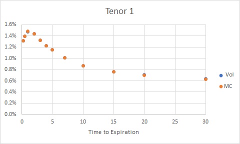
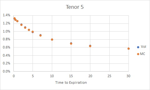
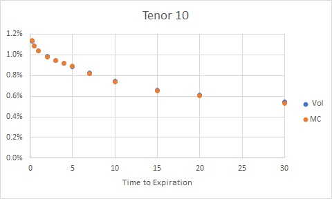
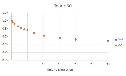
Figure 1: ATM Swaption Normal Volatilities.

This procedure leads to a good calibrated prices for all ATM swaptions, see Fig.1 where we compare input ATM volatilities with volatilities calculated from Monte-Carlo prices.

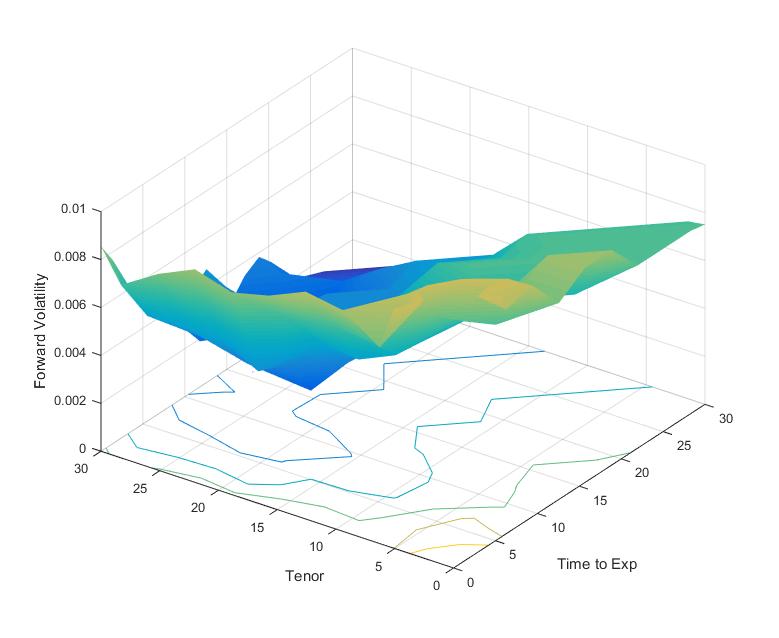
Figure 2: ATM Forward Volatility Surface.

Forward volatility surface is shown on Fig.2.

3 Sensitivity Calculation.

In the previous section we describe how to calibrate forward volatilities to reproduce all available ATM swaptions prices. This procedure can be applied to find forward volatilities calibrated to all swaption prices with shifted strikes from their ATM values.

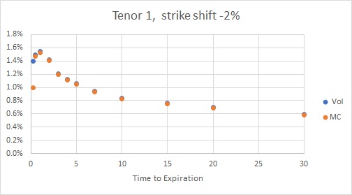
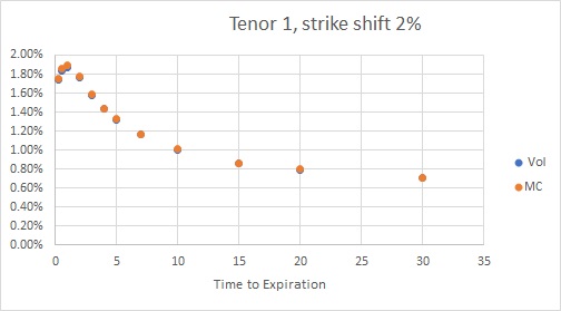
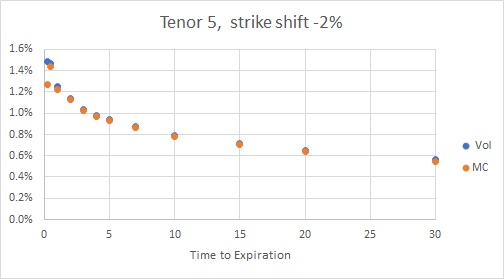
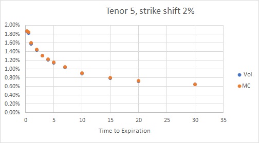
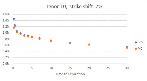
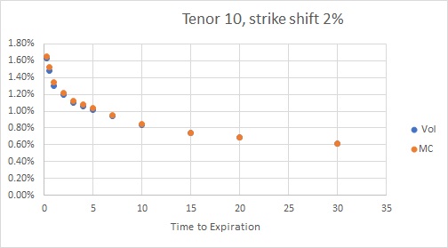
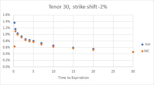
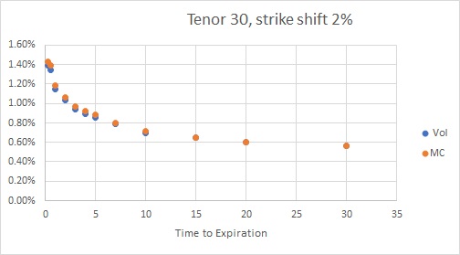
Figure 3: OTM Swaption Normal Volatilities.

Sswaption quotes are available within $\pm 2\%$ shifts. The calibration process is similar to the ATM swaption calibration. The only difference is a change of ATM volatility to the shifted one for selected strike. The calibration quality is good (see Fig.3).

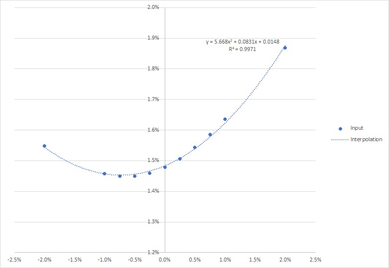
Figure 4: 1 Year Tenor 1. Swaption volatility smile.

In the selected data set for SOFR swaption volatility smile, we have strikes up to $\pm 2\%$ rate shift from ATM rate. This smile can be fitted by quadratic polynomial as it is demonstrated in Fig.4. Splines can also be used but obtained results are very similar. It means that we can use quadratic interpolation.

However, we need to take care of extrapolation, due to the swap rates can go out of $[-2\%,2\%]$ range rate shifts. This extrapolation need to be continuously differentiable and it would be very helpful if we can use extrapolation with limited volatility, in order to to use small volatility approximation.

We choose the following quadratic extrapolation:

$$v(x)=\alpha_{u}+\beta_{u}(x-x_{0})+\gamma_{u}(x-x_{0})^{2};\;\;\;x_{0}<x<x_{u};$$ (16)

$$v(x)=\alpha_{d}+\beta_{d}(x-(-x_{0}))+\gamma_{d}(x-(-x_{0}))^{2};\;\;\;x_{d}<x<-x_{0};$$

where $x_{0}=2\%$ is the current maximal available rate shift in input data; final points of extrapolation are chosen as $x_{d}=-10\%$ and $x_{u}=10\%$.

To obtain continuously differentiable function, we need to have

$$\alpha_{u}=v(x_{0});\;\;\;\alpha_{d}=v(-x_{0});$$

$$\beta_{u}=\frac{dv(x)}{dx}_{|x=x_{0}};\;\;\;\beta_{d}=\frac{dv(x)}{dx}_{|x=-x_{0}}.$$ (17)

To get zero slope at the end points $x_{u,d}$ we have

$$\gamma_{u}(x_{u}-x_{0})=-\frac{1}{2}\beta_{u};\;\;\;\gamma_{d}(x_{d}-(-x_{0}))=-\frac{1}{2}\beta_{d};$$ (18)

Above end points we assume that

$$v(x)=\left\{\begin{array}[]{ll}v(x_{d});&if\;x<x_{d};\\ v(x_{u});&if\;x>x_{u};\end{array}\right.$$ (21)

It leads to the smooth volatility curve depicted in Fig.5.

4 Fixed Tenor Dynamics

Before going to Scenario Generation Process let us consider fixed tenor dynamics. In the case of selected tenor $N$ we consider the following ATM swaption values distribution which present value is:

$$PV(S(T,N))=e^{-\int_{0}^{T}r(\tau)d\tau}\left(r_{ATM}(T,N)\sum_{n=1}^{N}B(T,T_{n})-1+B(T,T_{N})\right)=$$

$$=e^{-\int_{0}^{T}r(\tau)d\tau}\left(\frac{B(0.T)-B(0,T_{N})}{\sum_{n=1}^{N}B(0,T_{n})}\sum_{n=1}^{N}B(T,T_{n})-1+B(T,T_{N})\right).$$ (22)

In small volatility approximation Eq.(22) has the following form:

$$PV(S(T,N))=\Sigma(T,N)\xi\sqrt{T}.$$ (23)

In the case of non-zero constant difference between current swaption rate and ATM rate

$$\delta=r(T,N)-r_{ATM}(T,N);$$ (24)

swap present value distribution is

$$PV(S(T,N,\delta))=\delta\sum_{n=1}^{N}B(0,T_{n})+\Sigma(T,N,\delta)\xi\sqrt{T}=$$

$$=A(T,N)\left(\delta+\frac{\Sigma(T,N,\delta)}{A(T,N)}\xi\right);$$ (25)

where $\Sigma(T,N,\delta)$ is implied volatility of fixed tenor underlying for selected rate shift;

$$A(T,N)=\sum_{n=1}^{N}B(0,t_{n}).$$ (26)

As we can see from (25) we can use (5) to determine forward volatility assuming deterministic dependence of local forward volatility for selected point on the grid.

5 Local Volatility Scenarios

In the scenario generation process we can use formula for Local Volatility of normal volatility model. Here we assume that local forward volatility on every point on the grid can be defined deterministically from eq.(5). Below we describe this approach.

In addition to forward volatility, the formula depends on total variance $w$.

Deterministic variance can be calculated in the following form:

$$w(-2\%,n,k)=v_{f}^{2}(-2\%,n-1,k)dt+w(-2\%,n-1,k);$$

$$w(ATM,n,k)=v_{f}^{2}(ATM,n-1,k)dt+w(ATM,n-1,k);$$

$$w(2\%,n,k)=v_{f}^{2}(2\%,n-1,k)dt+w(2\%,n-1,k);$$ (27)

where $v_{f}(shift,n,k)$ is a forward volatility for selected time step $n$ and point on the grid $k$.

Then we use interpolation-extrapolation formulas to get function $w(x,n,k)$ for every point on the grid.

This procedure gives us all deterministic functions needed to calculate forward volatility according to equation (5).

To generate scenarios we need to calculate current swap rate which is a difference between current and initial ATM swap rates.

Initial ATM swap rate is:

$$r_{S}(0,t_{i},tenor)=\frac{B(0,t_{i})-B(0,t_{i}+tenor)}{\sum_{n=1}^{tenor}B(0,t_{i}+n)}.$$ (28)

Observed swap rate at time $t_{i}$ is:

$$r_{S}(t_{i},t_{i},tenor)=\frac{1-B(t_{i},t_{i}+tenor)}{\sum_{n=1}^{tenor}B(t_{i}+n)}.$$ (29)

So, the current rate strike is

$$X(t_{i},t_{i},tenor)=r_{S}(t_{i},t_{i},tenor)-r_{S}(0,t_{i},tenor).$$ (30)

In the case of $tenor=1$ we assume that this strike is the same for all time steps between $0$ and $tenor=1$. For $tenor=2$ we use strike for all times between $tenor=1$ and $tenor=2$ only etc.. As was mentioned in the previous section this procedure works. We use it because we already have calculated volatility sensitivities on swap rates. In calculations we apply calculated variance for selected strike and point on the grid (27).

We apply this procedure and generated 100,000 scenarios. ATM swaption prices for tenors 1, 5, 10 and 30 are shown in Fig.6.

1 Year Tenor 1 smile looks good (see Fig.7). All Tenor 1 expirations also in a good agreement with maximal errors for 5-year expiration, see Fig.8. All other expirations of Tenor 1 swaptions are in better agreement with the input prices, Fig.9.

Errors in higher tenors swaptions are smaller. You can see it in case of 5 Year Tenor 2 swaption, Fig.10.

Note, that using 1 month time step improve the quality of calibrated scenario set, see Fig.11.

6 Conclusion

Implementation of Local Volatility Model in interest rate model is presented. Calibration is deterministic, it works fast and is accurate. Observed short term and low tenor swaption errors can be improved by modifying scenario generation process.

Approach and results were presented on QuantMinds International Conference 2022, Barcelona, Spain [6].

FIGURES

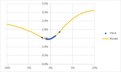
Figure 5: 1 Year Tenor 1 Volatility Extrapolation.

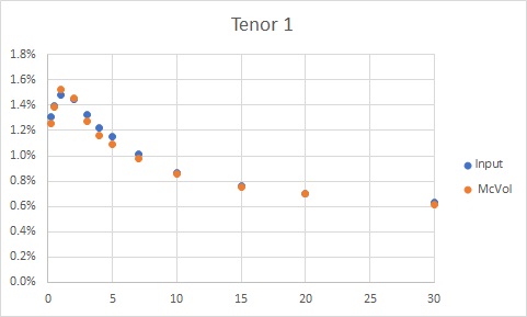
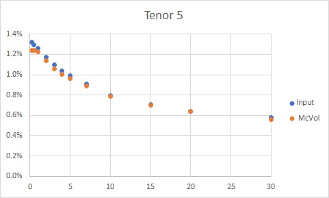
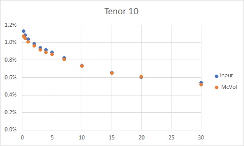
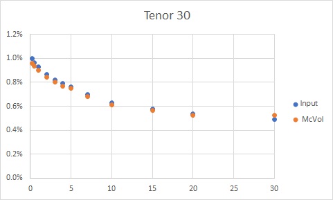
Figure 6: ATM Swaption Normal Volatilities with smile.

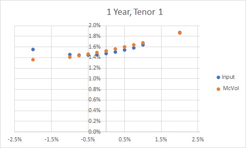
Figure 7: Swaption volatility smile.

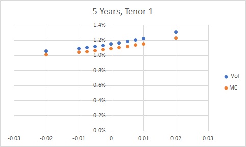
Figure 8: Swaption volatility smile.

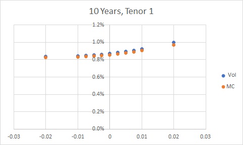
Figure 9: Swaption volatility smile.

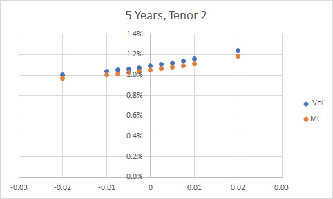
Figure 10: Swaption volatility smile.

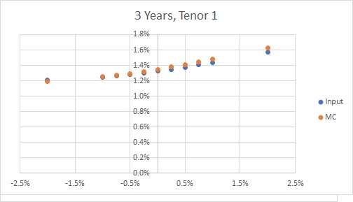
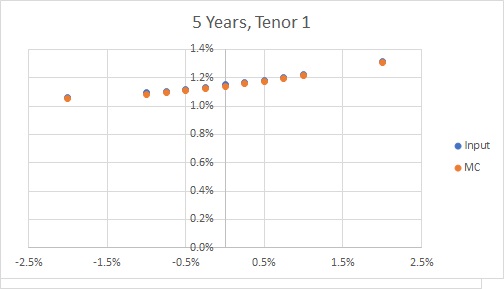
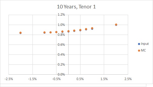
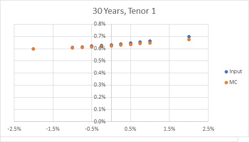
Figure 11: Swaption volatility smiles. 1 month time steps.

References

- [1] Dupire, B. (1994). ”Pricing With a Smile.” Risk 7, pp. 18-20.
- [2] Gatheral, J. (2006). ”The Volatility Surface: A Practitionerís Guide.” New York, NY: John Wiley & Sons.
- [3] Costeanu, V. & Pirjol D. ”Asymptotic expansion for the normal implied volatility in local volatility models” , arXiv:1105.3359v1, q-fin.CP, (2011);
- [4] V.M. Belyaev : “Swaption Prices in HJM Model. Nonparametric Fit”, arXiv:1697.01619, [ q-fin.PR], (2016); QuantMinds International Conferences (2017-2021);
- [5] Heath, D., R. Jarrow, and A. Morton (1990): ”Bond Pricing and the Term Structure of Interest Rates: A Discrete Time Approximation”.Journal of Financial and Quantitative Analysis, 25: 419440.
- [6] V.M. Belyaev : “Local Volatility in Interest Rate Models”, QuantMinds International Conference 2022, Barcelona, Spain.