All field emission experiments are noisy, … are any meaningful ?

Abstract

Representing field emission data on a Fowler-Nordheim plot is both very common and strongly not recommended. It leads to a spurious estimation of the emitter parameters despite a very good data fit. There is a lack of a reliable method of analysis and a proper estimation of the uncertainty in the extracted parameters. In this article, we show that the uncertainty in the estimation of the field enhancement factor or the emission area can be as high as $\pm 50\%$ even for a tungsten single emitter in good ultra-high vacuum conditions analyzed by the Murphy-Good model. Moreover, the choice of the exact Murphy-Good method can have a noticeable impact. We found that advanced analysis methods, based on the measurement of the differential conductance of the emitter, are so demanding in terms of emitter stability that up to now its requirements are probably out of reach in any field emission laboratory.

I Introduction

Vacuum electron sources have been at the heart of important applications such as electron microscopy, radio communication and electronics during the 20^th century. This led to extensive studies of the main electron emission mechanisms : thermionic emission,photo-emission, secondary emission and field emissionJensen (2017). By its very nature, field emission is probably the most intriguing process of the four. It is one of the first physical mechanisms involving the tunneling effect and is described by the so-called Fowler-Nordheim (FN) theoryFowler and Nordheim (1928). This model has had a great influence in the vacuum source community but also in fields as varied as molecular electronicsBeebe et al. (2006), chemistryBell (2013) or biologyDevault, Parkes, and Chance (1967). Despite its notoriety, the FN model is no longer recommended by the field emission communityForbes (2021). Furthermore, this model and its more exact version based on the Murphy-GoodMurphy and Good Jr (1956) theory (MG) has never been fully experimentally verified. We give in this article a brief overview of the past and recent attempts to close the gap between field emission theories and experiments. Then a set of experimental I-V curves from a tungsten emitter are extensively analyzed and the uncertainty in the extraction of physical parameters is estimated. The origin of these uncertainties is identified by determining the experimental noise, the current drift and comparison with various analysis methods. Finally, numerical simulations are performed in order to highlight the experimental difficulties and challenges to get more reliable field emission studies.

II A brief history of experimental verification of field emission theory

The misuse of field emission theory is probably as old as the questioning about its validity. There exists abundant literature on the subject and sometimes criticisms about the work of other researchers coexist in the same article with misuse of the theory by the author itself. In order to escape this pitfall, we will focus on what should not be done and cowardly avoid proposing a good method to test field emission.

II.1 The nightmare of the three parameters for field emission

For many experimentalists, it is well known that field emission experiments can be interpreted thanks to the FN theoryFowler and Nordheim (1928) which predicts that the current I is given by :

$$I=aS\frac{(\beta V)^{2}}{\phi}\exp(-b\frac{\phi^{3/2}}{\beta V})$$ (1)

where a and b are terms that depend only on universal physical constants, S is the emission area, $\beta$ is the field enhancement factor relating the applied voltage V to the electric field and $\phi$ is the work function. Then plotting the current in Fowler-Nordheim coordinates, (i.e. representing the logarithm of $I/V^{2}$ as a function of $1/V$) gives a straight line over several orders of magnitude. The goal is then to hope that an extraordinary value will be extracted from the slope and intercept of a linear fit, like a huge current density or $\beta$. Probably the most impressive attempt and the best example of the lack of reliability of this method can be found in ref. Feist, 1968 p.18. where a work function as ridiculously low as 0.01 eV was obtained. This is a point that is still too much ignored: there is no point in trying to publish about exceptionally low work function as this world record will be too hard to beat. One of the problems comes from the fact that Eq. 1 needs three parameters but only two (the slope and the intercept) can be extracted from the FN plot. It is then necessary to guess one of the parameters and often this guess is incorrect. Another issue in Eq. 1 is that it was obtained for a triangular tunneling barrier whereas the image charge has a huge effect on the barrier transparency. Using Eq. 1 will lead to an overestimation of the area by several orders of magnitude. It is then rather well known that MG theoryMurphy and Good Jr (1956) is more appropriate. In this article, for simplicity, other improvements of the model will be disregarded such as the replacement of the smooth flat surface hypothesis by a proper atomistic structure, the field and temperature dependence of the work function or the calculation of the electron density beyond the Sommerfeld free electron model.

Even with a more appropriate theory, many problems remain. For instance, it is sometimes considered that it is safer to take the work function as an input parameter and then to deduce S and $\beta$. The main reason is that a reasonable range of work function is between 3.5 and 6 eV whereas $\beta$ and S are related to the radius of curvature of the emitter and this radius can commonly vary between roughly one nanometer to several hundreds of nanometers. Nevertheless, some uncertainty in the work function remains and this uncertainty can have an important impact on the estimation of the other parameters. An interesting example was shown by MullerMüller (1955) where even in the apparently simple case of a 110 facet of an ultraclean field emitter the work function might differ by 0.5 eV depending on the annealing conditions (i.e. 1200^∘C versus 2200^∘C). To make this worse, it is highly unlikely that S, $\beta$ and $\phi$ are constant over the entire voltage range (see for instance ref.Jensen, 2017 chap. 30).

II.2 The longest IV curve

The most certain fact about field emission is that the current is dominated by an exponential term and a convincing proof has been given by Dyke and TrolanDyke and Trolan (1953) over seven orders of magnitude in current. However, It is more difficult to follow them when they claim that "The wave mechanical, image force corrected theory quantitatively predicted the observed average current density up to that density for which space charge dominated the emission." Although they provide numerical values for the field enhancement factor or the current density, it is hard to estimate if these values are quantitatively correct even when some margin of error of the order of 15 $\%$ is given. Their linear curves are not plotted in FN coordinates, they take into account the change of emission area with the voltage and despite their effort in terms of vacuum conditions (estimated below 10^-12 Torr), it can be seen in log scale that their current data points are not perfectly reproducible, with a difference in current sometimes higher than 10$\%$ and a deviation with the theoretical current density higher than 25 $\%$.

II.3 From qualitative to quantitative estimations

As it seems impossible to obtain reliable information from an I-V curve only, additional methods have been proposed. It was for instance proposed to perform a joint measurement of the current and the electron energy distributionYoung and Müller (1962); Young and Clark (1966). The width of the peak or the slope of the side below the Fermi energy should theoretically give an independent estimate of a relationship between $\phi$ and $\beta$. Although there isn’t a clear study of the uncertainties in this method, the stability of the emitter, peaks in the density of states not predicted by the free electron model and the resolution of the energy analyzer may limit its interest. It was also demonstrated that performing some measurements at different temperaturesYoung and Müller (1962) might be useful but it requires that the temperature dependence of the physical parameters does not complicate the interpretation. In ref.Van Oostrom, 1966, the different experimental and theoretical limits of field emission were rather well presented and several methods were proposed, for example, to determine the emission area with an impressive 2% uncertainty. Their conclusion was "that the Fowler-Nordheim model describes the experimental results satisfactory". In the book by ModinosModinos (1984), chapters 2.3 and 2.4 give a very good summary of different experimental attempts where it appears that the best estimate of the electric field and thus of $\beta$ has been done with an uncertainty as low as 3%. All these works are a clear improvement compared to analysis based only on the I-V curve and Eq. 1 but it does not allow to conclude on the closeness of these measurements with the real physical values, with maybe one exception that went almost unnoticed. In ref. Ehrlich and Plummer, 1978, an absolute current density measurement was performed on a tungsten <110>. The current was measured through a probe hole and the emission area was measured independently by field ion microscopy. The current density was then estimated with an uncertainty of about 70 %. This current density was compared to the theoretical values with and without image charge. The work function was considered to be between 4.5 and 6 eV and the value of $\beta$ was obtained from the slope of the FN plot. Despite these uncertainties, it was clearly shown that the absolute measurement of the current density lied between the triangular barrier theory and the image charge potential theoretical values. It was about 5 times lower than the image charge prediction and about 30 times higher than the triangular barrier prediction. From a metrological point of view, it can be said that there is room for improvement in field emission and that many experimentalists were too optimistic about the accuracy of their method. It might even be more correct to say that field emission experiments have a low accuracy but might show sometimes a good precision for inaccurate results.

II.4 And then came micro and nanotechnology

With the advent of nanosciences and their numerous poorly characterized materials and geometries, the risk was rather high that field emission experiments might lead to overwhelming spurious results. A call for standardization of field emission with an extensive list of mistakes to avoid was publishedZhirnov et al. (2001) rather early in the field but received less attention than several experimental works about supposedly exceptional nanoemitters. Probably, this battle could not be won in the absence of a good theory with a good method to analyze data. In the past years, new analytical formulae have been proposed to better describe experimental data Forbes (2008); Kyritsakis and Xanthakis (2015); Jensen (2019); Zubair, Ang, and Ang (2018); Liang and Chen (2008); Forbes (2010); Lachmann et al. (2021) requiring to measure the field emission current, the voltage derivative of the current, current fluctuations or the current noise. A fully open source tool is even availableKyritsakis and Djurabekova (2017) that includes corrections for small radius of curvature emitters. At even smaller scale, density functional theory calculations have been performed to estimate field emission currents at the atomic levelLepetit (2019); de Castro et al. (2019). Some theoreticians tried to compare their new calculations with experimental data but the lack of availability of good data make this task complicated. Some experimentalistsPopov et al. (2012); Feizi et al. (2012); Forbes et al. (2021); Ayari et al. (2021); Popov et al. (2022) showed that it was possible to plot new types of almost straight lines from their data. The term almost is chosen here to be vague enough to even include an FN plot appearing to be definitely not straightFeizi et al. (2012) and this is rather problematic. What useful information can be extracted from those plots remains an open questionForbes et al. (2021); Ayari et al. (2022). Very recently, a rather versatile webtool has been presented for data interpretationAllaham et al. (2022), but a simple version of the MG theory was used. In a preceding articleAyari et al. (2022) we showed that even for a flat emitter, some discrepancies between the different levels of approximations in standard field emission models might have an important impact on data analysis. In the next sections, we will apply these models to the analysis of field emission current and differential conductance of a simple tungsten emitter and compare their different results.

III Measurements on a banal tungsten emitter

Tungsten is the most and best-studied material in field emission and so it seems rather natural to test any new theory with it. With this material, the cleaning procedure can be pushed to its limit and at the same time, like most field emission emitters, it can get contaminated very quickly and present pronounced current instabilities. Thus this makes tungsten emitter, the perfect candidate to test the robustness of a theory towards noise in real conditions.

III.1 Experimental set up

A <111> tungsten tip, with an initial radius of about 15 nm, was fabricated by electrochemical etching of a 125 $\mu$m diameter tungsten wire. Field emission experiments were performed in a ultra-high vacuum chamber (see Fig.1) with a base pressure of $3\times 10^{-10}$ Torr. The tip was heated, several times, for 30 seconds, with a resisting loop at a temperature of 1700 K. The tip radius is expected to increase during the experiment due to these multiple heatings. An AC voltage of 1 VRMS at 33Hz and a variable DC voltage were applied on the tip with a bias tee. A quadrupole at zero bias was in front of the tip. The current was collected with a coupled microchannel plate (MCP)/phosphor screen system connected to a homemade current amplifier and a lock-in amplifier.

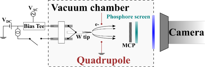
Figure 1: Experimental set-up used to perform the field emission experiments.

The role of the quadrupole was to shield the AC signal to avoid a cross-talk between the phosphor screen and the tip by capacitive coupling. The typical cross-talk current between the tip and the quadrupole in our system is 500 pA whereas the crosstalk between the tip and the phosphor screen is below our noise floor. Applying the AC voltage on the quadrupole and recording the alternative current on the tip would require a field emission current above 100 nA to make the cross-talk negligible. We preferred to apply the AC signal on the tip and to work at a lower current to reduce the changes over time in the morphology of the emitter. Such modifications occur due to surface diffusion, ion bombardment or adsorption of residual gazes and are strongly enhanced at a higher current. If the emitter changes are too important, it is not clear if the fitting of the data could be reliably compared with any model. Another advantage of working at low DC current is to reduce the 1/f noise (where f is the frequency of the noise). Indeed, surface diffusion on the tip induces a noise current roughly proportional to the square of the DC current and with a 1/f contribution to the current spectral density. As the measurement is very sensitive to any signal offset, it is important to reduce this contribution in the current measured by the lock-in amplifier.

The MCP/Phosphore allows visualization of any change of the emitter surface by recording the field emission pattern with a digital camera and at the same time to measure very low currents. We performed the measurements with DC field emission current in the fA to pA range. For a field emission current above 10 pA (corresponding to a current at the output of the MCP above several hundred nA), the amplification gain is not linear anymore. Before each measurement, we calibrated the offset for the DC and AC signal for zero applied DC voltage on the emitter. The DC offset is usually lower than 10 fA and the AC offset is lower than 10 aA.

III.2 Current and noise measurements

III.2.1 DC measurements

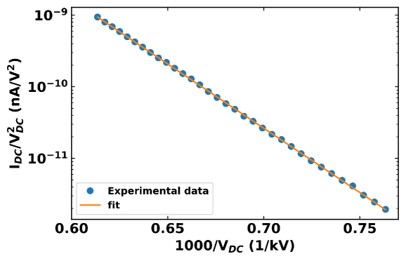
Figure 2: Typical Fowler-Nordheim plot of a <111> tungsten field emitter at a pressure of $3\times 10^{-10}$ Torr. The dots are the experimental data and the solid line is a linear fit. The coefficient of determination was R² = 0.999903 and the residual = 0.0108. The fitted slope is 41339 $\pm$ 73 V. The intercept is 4.57 $\pm$ 0.05 in natural logarithm. The standard deviation of the current compared to the fit is 1.82 % and the maximum deviation is around 6 % (see Fig.3).

Several voltage sweeps between 1300 V and 1630 V were performed. We have carried out data analysis using NumPy and SciPy Python packages. The data and programs used in this article can be found in the Zenodo data repositoryAyari (2022). In each case, we fitted independently the up and down sweeps of the standard Fowler-Nordheim plots of the data to a straight line (See figure 2) to extract the slope $A_{FN}$ and intercept $B_{FN}$ such that :

$$\log\frac{I}{V^{2}}=\frac{A_{FN}}{V}+B_{FN}$$ (2)

where $\log$ is the natural logarithm. Very good coefficients of determination R² between 0.9993 and 0.9999 were obtained. The deviation $\Delta I(V)/I$ of the experimental DC current $I(V)$ to the fit $I_{fit}(V)$ (figure 3) was calculated for each applied voltage where:

$$\Delta I(V)/I=\frac{I(V)-I_{fit}(V)}{I(V)}$$ (3)

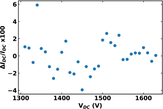
Figure 3: Relative deviation (Eq.3) of the experimental direct current I(V) from its fit shown in Fig 2.

Its maximum value is lower than 10 $\%$ and its standard deviation is between 1.8 and 4.4 $\%$ depending on the voltage sweeps. In this article, we plot only the data from the voltage sweep showing the lowest standard deviation and best R² but the other data sets give somewhat similar results. From Fig. 3, it might seem that for this run the emitter has a current Gaussian noise of a few percent and a maximum deviation of 6 $\%$. However, Fig. 3 hides the presence of a current drift in the emitter. This can be observed for instance by comparing the current at the same voltage for different voltage sweeps as shown in Fig. 4. This drift is in the order of 8 $\%$ per hour which corresponds roughly to 1.5 $\%$ for the duration of a single voltage sweep.

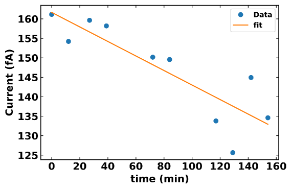
Figure 4: Field emission current as a function of time measured at an applied voltage of 1470V for each voltage sweep. The dots are the experimental data and the solid line is a linear fit.

In standard experimental field emission articles, both values of current noises (Gaussian noise and drift) are generally not shown, whereas they are crucial to estimate the reliability of the fit of a Fowler-Nordheim plot. Instead, the current stability versus time for several series of fixed voltages is sometimes presented. This doesn’t guarantee that the current will be the same and so the emitter will be identical when the initial voltage value is applied again. The sample might change quickly after applying a higher voltage value and the data of this evolution are sometimes simply removed. The noise values, we have obtained are rather common in good vacuum conditions, but it is not clear if this is good enough to perform a reliable estimate of the emitter parameters. In the next sections, we will try to answer to this point after analyzing our data and performing some simulations.

III.2.2 Differential Current

The derivative of the current can be obtained by numerical differentiation but also with a lock-in amplifierSpindt et al. (1976). A first-order Taylor expansion of the expression of the current shows that as long as the AC voltage is not too high, the current measured on a lock-in amplifier at the modulation frequency is directly proportional to the derivative of the direct current. It is usually considered that numerical differentiation methods are noisier than lock-in methods. We fitted the derivative of the current obtained by both methods and calculated their respective deviations from the fitted data in order to compare their noises. As the derivative of the current has a similar voltage dependence as the current itself, we chose to make a linear fit of the logarithm of $\partial I/\partial V\times 1/V^{2}$ as a function of $1/V$. The standard deviation of the lock-in signal compared to the fit is between 4 and 10 $\%$ depending on the different voltage sweeps, approximately twice as big as the DC noise. The noise of the current derivative obtained by numerical differentiation is systematically bigger than the lock-in measurement with an excess noise at best 15 $\%$ higher than the standard deviation of the lock-in data. In the worst case, the noise from the numerical derivative was 4 times bigger than the lock-in noise. The case with 15 $\%$ excess noise is presented in Fig. 5. Although a more systematic study would be necessary, we do not consider that most of the noise in the current derivative is coming from the 1/f noise as the coefficient of correlation between the current and its derivative do not present a clear trend and varies between 0.18 and 0.68 from one voltage sweep to another. The fact that the relative lock-in noise is higher than the relative DC noise is probably due to the low amplitude of the lock-in current. For an AC voltage of the order of one volt, the lock-in current is typically between one and two orders of magnitude lower than the DC. We will see that this level of noise in the voltage derivative of the current is an important limitation to the use of advanced field emission analysis combining the current and its derivative.

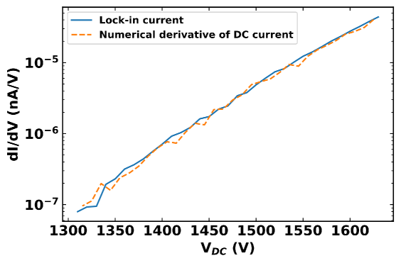
Figure 5: Lock-in current (solid line) for an applied AC voltage of 1V as a function of the applied DC voltage and numerical derivative (dashed line) for the same voltage sweep as in Fig. 2.

IV Data analysis

In this section, several analysis methods will be tested on the data presented above. The different predictions between different runs and different methods will be highlighted.

IV.1 Traditional analysis methods

As explained above, once a convincing fit such as the one in Fig. 2 is obtained, an additional hypothesis is necessary to draw some conclusions. As our emitter is a <111> tungsten, it is plausible that its work function is close to 4.5 eV but other work function values will be tested too. Our goal here is first to estimate the uncertainty arising from the analysis of a single data set and then to compare it with the experimental statistical uncertainty coming from the full data set.

IV.1.1 Analysis with a fixed work function

If we assume that the work function $\phi$ = 4.5 eV, we can determine the value of $\beta$ and S provided we define the field emission model we want to use. In the following, we will estimate $1/\beta$ (which gives more convenient numerical values than $\beta$) and the area from the data presented in Fig. 2 with seven different methods based on several field emission models. The results are gathered in Fig. 6.

The simplest model to use is the triangular barrier model with Eq. 1 where $\beta$ is deduced from the negative slope of the FN plot $A_{FN}$:

$$\beta=-\frac{b\phi^{3/2}}{A_{FN}}$$ (4)

We obtained $1/\beta=634\pm 1$ nm. Just to have a rough idea of the size of the tip, we can use the Gomer formulaGomer (1955) $\beta=1/5r$ (see also ref. de Assis, Dall’Agnol, and Forbes, 2022 for an excellent review on the subject) where $r$ is the radius of curvature of the emitter. This radius at the apex is then equal to 126.8 $\pm 0.2nm$. This value is sufficiently high so that the correction factor for sharp tips as proposed in ref. Kyritsakis and Xanthakis, 2015 will not be necessary. The area of emission can be easily obtained from the intercept $B_{FN}$ of the FN plot:

$$S=\frac{\phi}{a\beta^{2}}\lim_{\frac{1}{V}\to 0}\frac{I}{V^{2}}=\frac{\phi}{a\beta^{2}}\exp(B_{FN})$$ (5)

This area is equal to 114213 nm² although it is known that this value is much too high as will be confirmed below.

The next six methods will include the image charge correction. The current in its simplest form at 0 K is given by:

$$I=JS=aS\frac{(\beta V)^{2}}{\phi}\exp(-bv(y)\frac{\phi^{3/2}}{\beta V})$$ (6)

where a and b are the same terms as in Eq.1, J is the current density and $v(y)$ is the barrier shape correction factor that depends on the applied electric field through the variable $y$ and can be expressed as a combination of elliptic integrals. $v(y)$ can be simplified using this approximationForbes (2006)

$$v(y)\approx 1-y^{2}+\frac{y^{2}}{3}\log(y)$$ (7)

So for our second method, we used Eqs. 6 and 7 and perform a least square fitting of the data with these equations. We obtain $1/\beta=650$ nm and S = 573 nm². It is also possible to have an estimation of the emission half angle $\theta$ about $6^{\circ}$ using the Gomer formula and Eq. 14 in ref. Dyke and Dolan, 1956:

$$S=2\pi r^{2}(1-\cos\theta)$$ (8)

For the third method, we performed the same analysis but without the approximation from Eq. 7 i.e. we use the exact expression from the MG modelMurphy and Good Jr (1956). We obtained $1/\beta=651$ nm and S = 575 nm² which are very close to the values obtained with the second model.

For the other methods, we will use the value of the slope of the FN plot instead of performing a direct non-linear fitting of the data. It is known that image charge models will not give a straight line in FN coordinates but it is anyway a common method as the deviation from a straight line is hardly visible. However, this method requires some care as the relationship between the slope of the fit and the term in the exponential in the expression of the current is not as obvious as it first seems. The fitted slope in FN coordinates must be compared to the voltage derivative of the current and not to the term in the exponentialHouston (1952). Thus the expression of $\beta$ is now:

$$\beta=-\frac{b\phi^{3/2}}{A_{FN}}s(y)$$ (9)

where $s(y)=v(y)-\frac{y}{2}\frac{\partial v(y)}{\partial y}$.

For the fourth method, the value of $y$ and thus $\beta$ will be deduced self-consistently. First, a value of the voltage must be chosen to compare the slope of the FN plot to the derivative of the current at this voltage point. It seems reasonable to choose a voltage at the center of the FN plot which corresponds to the mean of the inverse of the applied voltages, but here, as it has little influence, we will prefer a voltage value $V_{m}$ in the center of the applied voltage range equals to 1470 V. We started the iterative process with the value of beta obtained from the preceding method. As $y$ depends on the electric field, this new $\beta$ gives $y$ and $y$ will give a new value of $\beta$ according to Eq. 9. After few iterations, we obtain $1/\beta=653$ nm. The value of $y_{m}$ is equal to 0.4 and $s(y_{m})$ = 0.97. It is interesting to notice that $s(y)$ is close to 1 which explains why the values of $\beta$ with or without the image charge correction are very close although the value $v(y_{m})$ = 0.79 has a huge influence in the values of the current density and the emission area. After some calculations, it can be shown that the emission area is given by:

$$S=\frac{\phi}{a\beta^{2}}\exp(b\frac{\phi^{3/2}}{\beta V_{m}}(v(y_{m})-s(y_{m})))\times\lim_{\frac{1}{V}\to 0}\frac{I}{V^{2}}$$ (10)

and is equal to 615 nm². It is also possible to obtain the area by dividing the measured current by the current density J from Eq. 6. It can be calculated for each voltage point and averaged. It gives an emission area of 616 nm². So both variants to get the area are equivalent and only the first one will be used in the rest of the article.

In the fifth method, instead of using an iterative method, the value of $\beta$ that satisfies this equation is solved numerically:

$$|A_{FN}|=|\frac{\partial log(I/V^{2})}{\partial 1/V}|=V_{m}\left[\frac{V_{m}}{J(\beta,\phi,V_{m})}\frac{\partial J(\beta,\phi,V_{m})}{\partial V}-2\right]$$ (11)

with J the current density in Eq. 6. In this case, Eq. 11 is strictly equivalent to Eq. 9 but Eq. 11 can also be used for another expression of J. We obtained $1/\beta=653$ nm, an identical value compared to the iterative method. The area is given by rewriting Eq. 2:

$$S=\frac{V_{m}^{2}}{J(\beta,\phi,V_{m})}\exp(B_{FN}+\frac{A_{FN}}{V_{m}})$$ (12)

and gives also an identical value compared to the iterative method. For the last two methods, the general MG equation will be used (Eq. 19 in ref. Murphy and Good Jr, 1956) as we showedAyari et al. (2022) that this equation predicts a substantially different exponent in the pre-exponential term in the current compared to Eq. 6. So, to determine $\beta$ for the sixth method we will solve Eq. 11 and to determine the area Eq. 12 will be used but with the full MG equation at T = 0 K integrated numerically. For the last method, the same calculation is performed but at 300 K. We obtain $1/\beta=654$ nm and S = 726 nm² for the sixth method at 0 K and $1/\beta=656$ nm and S = 748 nm² for the last method at 300 K.

As can be seen in Fig. 6, the different methods with the image charge potential, extract fairly similar values of $\beta$ differing by less than 1 $\%$ but are not very consistent regarding the emission area as they differ by more than 20 $\%$. We deduced these physical effective parameters by making the hypothesis that the work function was known. As the <111> facet has a low density, it is very reactive even in UHV and thus it can quickly adsorb residual atoms which might change its work function. A possible value of $\phi$ can be 5.0 eV. So, the same analysis can be performed with this new reasonable work function, to see how the new estimated $\beta$ and S deviate from the preceding values. This alternative analysis gives essentially the same results for the emission area: for the third method, we obtained S = 583 nm² instead of 575 nm² for 4.5 eV and for the last method we obtained S = 755 nm² instead of 748 nm² for 4.5 eV. Of course, the extracted values of $\beta$ change significantly as the work function changes by 10 $\%$. It might be deduced from the dispersion of the data in Fig. 6, that analysis with a more accurate model tends to predict bigger $1/\beta$ and S. To the contrary, a more reliable optimization protocol that consists of using a direct least square fitting of the data instead of relying on the slope and intercept of an FN plot tends to predict lower $1/\beta$ and S.

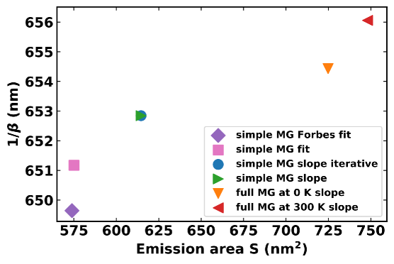
Figure 6: Inverse of the enhancement factor $\beta$ as a function of the emission area S extracted from different methods of analysis. The method based on the triangular barrier is not represented as it predicts an area two orders of magnitude too high. The caption listed from top to bottom the different models by order of appearance in IV.1.1.

IV.1.2 Analysis with a fixed method

Although we consider that the choice among the different analysis methods is a matter of habit and a compromise between the acceptable level of complexity versus the required accuracy, we will decide somewhat arbitrarily to use the fifth method based on the simple MG equation (Eq. 6) and the slope of the FN plot. It gives predictions in the middle range of the other methods and it is close to what is probably the most used method among the experimentalists that accept to go beyond the oversimplified triangular barrier model.

Before the experiment, the tip radius was estimated to be 15 nm from scanning electron microscope (SEM) imaging, but the value we deduced from the preceding analysis was around 130 nm. This difference can partly be explained by the heating protocol used to obtain a clean tip which leads to tip blunting. However, if we had based our analysis on considering the SEM image radius as correct and used the Gomer formula to consider $\beta$ as an input parameter, a work function of 18.86 eV would have been obtained. This result is obviously completely wrong. Such a mistake is usually done the other way around. Often the radius of curvature is overestimated (and beta is thus underestimated) for large and dirty tips that tend to form protrusions having a much smaller radius of curvature than the initial tip. This leads to an incorrect value of the work function particularly low.

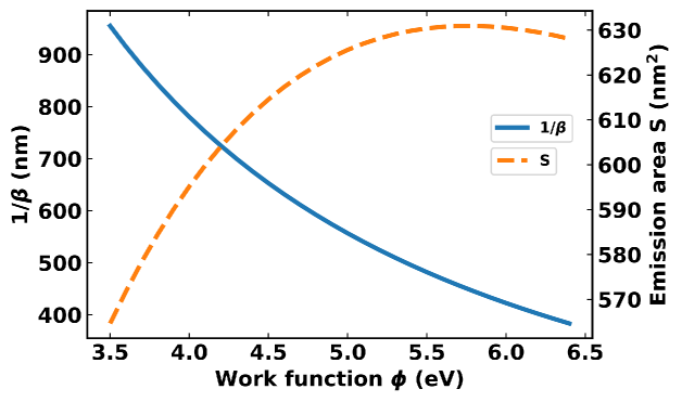
Figure 7: Inverse of the enhancement factor $\beta$ (solid line) and emission area S (dashed line) as a function of the work function from the simple MG slope method of analysis.

Although it is not possible to extract S, $\phi$ and $\beta$ from an I-V characteristic only, it is sometimes consideredCharbonnier and Martin (1962); Van Oostrom (1966); Forbes (1999) that it is possible to obtain a good estimate of the emission area by fitting the I-V characteristic and varying the work function over a reasonable range of physically possible values. In Fig.7, such an analysis was performed on our data for a work function range between 3.5 and 6.5 eV (i.e. 5eV $\pm 30\%$). We didn’t find the same precision as in ref. Van Oostrom, 1966, although the variations of the estimation area are quite acceptable and lower than the dispersion we found between the different methods of analysis in IV.1.1. We obtained a value of the area of emission of 598 $nm^{2}\pm 5.5\%$. The uncertainty is slightly lower than the one mentioned in ref. Forbes, 1999 or ref. Charbonnier and Martin, 1962 who reported respectively at best $\pm 9\%$ and $\pm 7\%$. Interestingly, even with an estimation error of the area of emission as low as $\pm 5.5\%$, the uncertainty on the 2 other parameters is still important, in particular, the error on $1/\beta$ is still $\pm 43\%$. In a way, the problem of having three physical parameters for two parameters extracted from the fit is more of a question of having two physical parameters ($\beta$ and $\phi$) for one fit parameter.

Now that we have an idea of the uncertainty on a single measurement voltage sweep due to the analysis, we can evaluate the uncertainty due to the evolution of the emitter. We performed the extraction of S and $\beta$ from the fifth method of analysis (MG simple slope) for two different work functions values between which the emitter work function is very likely to be (i.e. 4.5 and 5 eV). The area between the dotted curve for $\phi$ = 4.5 eV and the diamond curve $\phi$ = 5 eV in Fig. 8 can be considered as the zone where the emitter parameters are likely to be found. We observed a significant modification of the area of emission by a factor of 4 and the maximum change in the estimated area between 2 successive voltage sweeps can be higher than 300 nm². The experimental drift in $\beta$ is moderate and the uncertainty in the work function is the dominating issue.

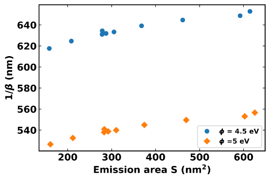
Figure 8: Inverse of the enhancement fact $\beta$ as a function of the emission area S extracted from the simple MG slope method of analysis. The dots are for a work function $\phi$ = 4.5 eV and the diamond are for 5 eV.

It can be concluded from this section that the uncertainty in the estimation of the emission area is firstly dominated by the temporal evolution of the emitter, then by the uncertainty in the analysis method and is little influenced by the uncertainty on the work function. Regarding the uncertainty in $\beta$, it doesn’t come from the uncertainty in the measurement of the current or the choice of the analysis methods but it is related to the uncertainty in the value of the work function. There is a need for a complementary measurement capable to give a reliable and independent value of $\beta$ or $\phi$. All these aspects taken into account, the uncertainty in both S and $\beta$ is of the order of $\pm 50\%$.

IV.1.3 Advanced data analysis

In the past few years, several new methods of data analysis have been proposed that could help to extract additional information from experimental data. One of these new methodsZubair, Ang, and Ang (2018) takes into account the roughness of the vacuum interface and proposes that field emission is described by:

$$I=CV^{2\alpha}\exp(-B/V^{\alpha})$$ (13)

where C and B are constant and $\alpha$ is a fractional space dimensionality parameter with $0<\alpha\leq 1$ which can be reformulated into:

$$\frac{dI}{dV}\frac{V}{I}=2\alpha+\frac{\alpha}{V^{\alpha}}B$$ (14)

Thus, plotting $\frac{dI}{dV}\frac{V}{I}$ as a function of $1/V^{\alpha}$ should give a straight line. Such a plot cannot be obtained so easily as $\alpha$ is unknown. Surprisingly, the authorsZubair, Ang, and Ang (2018) proposed a rather crude method, to say the least, that consists of plotting the left hand-side of Eq. 14 as a function of $1/V$. They applied it even for a situation where they found an $\alpha$ of 0.4. Here, we will prefer to plot the left-hand side of Eq. 14 as a function of $1/V^{\alpha}$ for different values of $\alpha$ and select the plot with the lowest least square fitting. An appealing aspect of Eq. 14 is that for the best fit, the intercept should also give $2\alpha$. So we have a nice way of checking the consistency of the theory. We have seen that in our set-up the measurement of the derivative of the current is roughly twice noisier than for the DC. Nevertheless, the product of this differential conductance by the resistance is relatively well defined as shown in Fig. 9 with a roughly linear trend if the first low voltage noisy points are excluded. The values of $\alpha$ are not reliable as it gives the best least square fitting for values between -9 and 16.6. depending on the analyzed voltage sweep. The coefficient of determination $R^{2}$ is rather low, the best sweep gives $R^{2}$ = 0.83 (in Fig. 9, $R^{2}$ = 0.79) and its lowest value was 0.3. Finally, the value of $\alpha$ obtained from the intercept shows no correlation with the $\alpha$ obtained from the least square fitting and varies between 9.7 and 27.7. So the data are probably too noisy to give a reliable value and the $\alpha$ we obtained is strongly out of the expected range between 0 and 1.

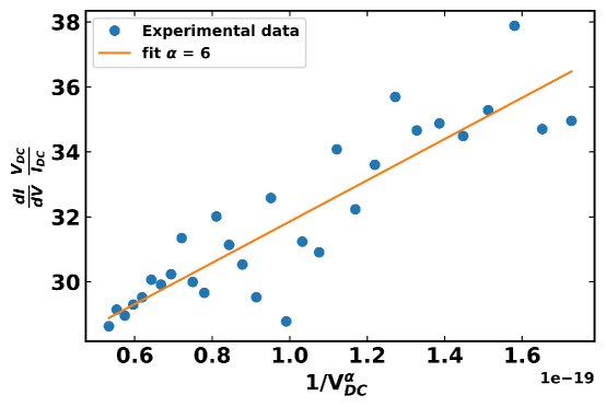
Figure 9: Variation of the product of the differential conductance by the resistance as a function of the inverse of the DC voltage at a power 6 corresponding to the best fit for Eq. 14 for the same voltage sweep as in Fig. 2.

Another method is based on a new analytical formula for the field emission current proposed by ForbesForbes (2008). The formula was obtained for the case of a tunneling barrier with a classical image charge correction and can be expressed as:

$$I=a_{\kappa}S\frac{(\beta V)^{\kappa}}{\phi}\exp(-b\frac{\phi^{3/2}}{\beta V})$$ (15)

where $\kappa$ and $a_{\kappa}$ are independent of V and $\beta$, but vary with the work function. Now, a plot of the logarithm of $I/V^{\kappa}$ as a function of 1/V should give a straight line and a better fit of the experimental data. Again, as $\kappa$ is unknown, such an exact plot cannot be directly obtained. Moreover, according to more exact models, $\kappa$ is not that constant on a large voltage rangeAyari et al. (2021) or because of the contribution of additional effectsFilippov et al. (2022). Despite, these significant drawbacks, the question of whether $\kappa$ might be a useful empirical parameter remains open. In order to estimate this $\kappa$, it was proposed to plot the logarithm of $I/V^{\kappa}$ as a function of 1/V with different $\kappa$ values to check which one gives the best fit to the data. We performed linear fits of the logarithm of $I/V^{\kappa}$ as a function of 1/V for different values of $\kappa$. The best least square fitting gave highly fluctuating values of $\kappa$ ranging from -4 to 13 depending on the voltage sweeps but very good coefficients of determination. For the data presented in Fig. 2, the corresponding $\kappa$ is 5 with a coefficient of determination 0.99989. It means that although 99.989 $\%$ of the variance in the logarithm of $I/V^{\kappa}$ can be explained by the changes in 1/V according to the model, the best-extracted value of $\kappa$ is unreliable. A hint on the lack of confidence, we can have in this fit is that the value of $\kappa$ obtained from the least square fitting doesn’t correspond to the maximum of the coefficient of determination, obtained here at $\kappa$ = 1.8.

$\kappa$ can also be estimated by measuring the voltage derivative of the current because Eq. 15 leads to the following expression:

$$\frac{V^{2}}{I}\frac{dI}{dV}=b\frac{\phi^{3/2}}{\beta}+\kappa V$$ (16)

So a plot of this ratio as a function of V should be linear with a slope giving directly the value of $\kappa$. We found a not very convincing agreement between this expected linear behavior and our data (see Fig. 10). We have performed a linear fit for different voltage sweeps and extracted from the slope a value of $\kappa$ between -11 and +15. At first sight, it seems surprising that Fig. 9 shows a visible trend with the voltage whereas in Fig. 10 the trend is drowned in the noise as they only differ by a multiplicative V term. This apparent discrepancy comes from the fact that in equation 16, the constant term is at least an order of magnitude bigger than the variation of the voltage-dependent term. So in Fig. 10, the data represents a signal with a big intercept and a small varying term whereas in Fig. 9, the data represents a signal with a small intercept and a big varying term.

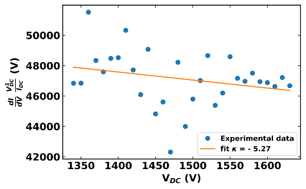
Figure 10: Variation of the expression of the left-hand side of equation 16 as a function of the applied DC voltage. A linear fit of the curve gives $\kappa$ = -5.27

Using differential conductance to extract additional information imposes stringent conditions on the acceptable level of noise. We estimated in the previous section that our uncertainty on the value of $\beta$ or S was about $\pm 50\%$ whereas in this section the fluctuations might be up to 10 times bigger than the expected value of $\kappa$. This raises the question of how much noise is acceptable to make a reliable measurement. In the last section, some simulations will be performed with a tunable level of noise to give some hints about the relation between the current noise amplitude and the uncertainty in extracted physical parameters.

V Numerical simulations in the presence of noise

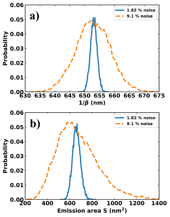
Figure 11: a) Distribution of $1/\beta$ for a noise level of 1.82 $\%$ (solid line) as in experiments and 5 times bigger (dashed line). b) Distribution for the emission for the same conditions as in a).

In III.2, the current noise level was estimated with a Gaussian noise contribution and long-term drift. In the following simulations, the current drift will not be taken into account. The main reasons are i) the Gaussian noise contribution explains already the main uncertainty in the estimation of the parameters; ii) properly reproducing the drift requires a random walk approach with too many unknown parameters to model the current drift and its derivative for all voltage points. To keep it simple, we started by calculating the emission current for $\phi$ = 4.5 eV, S = 659 $nm^{2}$ and $1/\beta$ = 653 nm with the simple MG formula (Eq. 6) on the same voltage range as our experiments. Then, each calculated current point is multiplied by a different randomly generated number from a normal distribution. The standard deviation of the distribution was chosen equal to 1.82 $\%$, identical to the noise value for the data shown in Fig. 2. The noisy calculated current is fitted in order to extract the slope and intercept of an FN plot. $\beta$ and S are calculated by the fifth method as in IV.1.2. This procedure is reproduced 10 000 times and a histogram of the extracted values is obtained (see Fig.11). For a noise value of 1.82 $\%$, the standard deviation of the distribution of $1/\beta$ is 0.17 $\%$ and 5.3 $\%$ for the emission area. Thus, for such a level of Gaussian noise, the uncertainty induced on $\beta$ and S is not the dominant contribution and its impact is comparable to the uncertainty related to the choice of the analysis method as in Fig.6. An increase of the noise by a factor of 5 increases the distribution width of $1/\beta$ and S by the same amount. It can be noticed however that the distribution of emission area in Fig.11 b) is not Gaussian anymore for such a high level of noise. The peak maximum is shifted toward a lower value but the mean is up-shifted by 20 nm². So beyond a certain noise level averaging over several experiments might lead to an overestimation of the area.

Gaussian noise was also added to the voltage derivative of the current and the value of $\kappa$ was obtained by the same method as in Fig. 10. The simulations were performed 10 000 times for three different noise levels: i) a current noise with a standard deviation of 1.82 $\%$ and noise of the derivative of the current with a standard deviation of 8.347 $\%$ as in the experimental data presented in the figures 2, 5 and 10; ii) a current noise and voltage derivative of the current noise both equal to 1.82 $\%$; iii) a current noise and voltage derivative of the current noise both equal to 0.1 $\%$. In Fig. 12, it appears clearly why in our experimental conditions the value of $\kappa$ had a huge uncertainty as the simulated $\kappa$ = 1.2 $\pm 7$ ($\approx\pm 550\%$). As the averaged value is close to the expected value, it can be argued, that performing several measurements might converge toward a reliable measurement. However, with such a level of noise, it would require about 3000 measurements to have an uncertainty below 10 $\%$. Even if a single measurement was as short as one second, the current drift and thus the changes in the emitter properties might be too important. In the case where the noise in the differential conductance is reduced down to the same value as the current noise (i.e. 1.82 $\%$), $\kappa$ = 1.2 $\pm 2$ which is still too high. It requires to have both noises as low as 0.1 $\%$ to be in acceptable conditions where $\kappa$ = 1.18 $\pm 0.12$. However, such a low level of noise is very hard to reach experimentally. The extraction of $\kappa$ seems to require an ultra-stable emitter in an ultra-clean UHV environment. For example, It might be better to perform such measurements from a W crystal plane with lower Flicker noise like the <110> orientationSwanson and Crouser (1967); Swanson and Schwind (2009) and in extreme UHV with a vacuum level in the 10^-11 Torr range or below. After such improvements other factors might become dominant such as shot noise, vibrations, sensitivity of the detection, heating effects or temperature drifts. All these limiting factors would require to be precisely quantified, but are beyond the scope of this article.

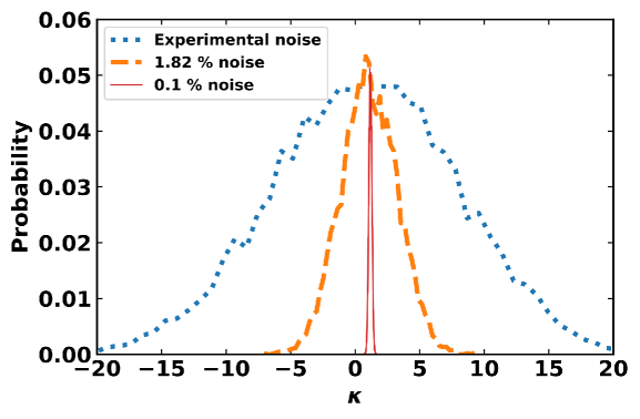
Figure 12: Distribution of $\kappa$ for a noise level similar to the data in Fig. 2 (dotted line), a noise level of 1.82 $\%$ (dashed line) and 0.1 $\%$ (solid line).

VI Conclusion

Field emission data on tungsten single emitter were analyzed using the Fowler-Nordheim model and different Murphy-Good approximation models. We showed that slight differences between traditional analysis methods using Murphy-Good approximation can give significant differences, in the order of 10$\%$, in the estimation of the emission area S. The uncertainty on beta of the order of 50 $\%$ remains dominated by the uncertainty in the value of the work function. Without an independent measure of $\beta$ or $\phi$, there is little hope to reduce this uncertainty. This partial conclusion is not especially new, but it was maybe useful to underline it with the example of a simple emitter. In our experimental UHV conditions, the drift and fluctuations of the emitter have small consequences on the value of $\beta$ but lead to an important variation of the emission area of the order of 50 $\%$. Regarding more advanced and recent analysis methods, necessitating the combination of current and differential conductance measurements, we have observed that our results were unreliable whereas our noise level is reasonable. Numerical simulations showed that the level of Gaussian noise acceptable to obtain reliable analysis is extremely low with a standard deviation of the order of 0.1 $\%$. Such an experiment might be feasible at low temperatures, with better electronics and selecting particularly stable facets with a probe hole.

This quest for a better agreement between theory and experiment is probably the most important intellectual challenge in field emission. At the same time, it may appear to be of little practical interest because it could lead to overly complex analytical formulas or theoretical approaches. However, it clearly deserves better attention from the whole field emission community because it is also a quest toward more stable emitters; a problem of paramount importance for applications. For example, the main reason why cold cathodes despite their higher brightness are not widely used in electron microscopy is their lack of stability.

Conflict of interest

The authors have no conflicts to disclose.

DATA AVAILABILITY

The data that support the findings of this study are openly available in Zenodo at

https://doi.org/10.5281/zenodo.7215660, Ref. Ayari, 2022

References

- Jensen (2017) K. L. Jensen, Introduction to the physics of electron emission (John Wiley & Sons, 2017).
- Fowler and Nordheim (1928) R. H. Fowler and L. Nordheim, “Electron emission in intense electric fields,” Proceedings of the Royal Society of London. Series A, Containing Papers of a Mathematical and Physical Character 119, 173–181 (1928).
- Beebe et al. (2006) J. M. Beebe, B. Kim, J. W. Gadzuk, C. D. Frisbie, and J. G. Kushmerick, “Transition from direct tunneling to field emission in metal-molecule-metal junctions,” Physical review letters 97, 026801 (2006).
- Bell (2013) R. P. Bell, The tunnel effect in chemistry (Springer, 2013).
- Devault, Parkes, and Chance (1967) D. Devault, J. H. Parkes, and B. Chance, “Electron tunnelling in cytochromes,” Nature 215, 642–644 (1967).
- Forbes (2021) R. G. Forbes, “21st century planar field emission theory and its role in vacuum breakdown science,” arXiv preprint arXiv:2107.08801 (2021).
- Murphy and Good Jr (1956) E. L. Murphy and R. Good Jr, “Thermionic emission, field emission, and the transition region,” Physical review 102, 1464 (1956).
- Feist (1968) W. Feist, “Cold electron emitters,” Electron Beam and Laser Beam Technology 4 (1968).
- Müller (1955) E. W. Müller, “Work function of tungsten single crystal planes measured by the field emission microscope,” Journal of Applied Physics 26, 732–737 (1955).
- Dyke and Trolan (1953) W. P. Dyke and J. Trolan, “Field emission: large current densities, space charge, and the vacuum arc,” Physical Review 89, 799 (1953).
- Young and Müller (1962) R. D. Young and E. W. Müller, “Progress in field-emission work-function measurements of atomically perfect crystal planes,” Journal of Applied Physics 33, 91–95 (1962).
- Young and Clark (1966) R. D. Young and H. E. Clark, “Effect of surface patch fields on field-emission work-function determinations,” Physical Review Letters 17, 351 (1966).
- Van Oostrom (1966) A. G. J. Van Oostrom, “Validity of the fowler-nordheim model for field electron emission,” Philips Research Reports 1, 1–100 (1966).
- Modinos (1984) A. Modinos, Field, Thermionic, and Secondary Electron Emission Spectroscopy (Springer, 1984).
- Ehrlich and Plummer (1978) C. Ehrlich and E. Plummer, “Measurement of the absolute tunneling current density in field emission from tungsten (110),” Physical Review B 18, 3767 (1978).
- Zhirnov et al. (2001) V. Zhirnov, C. Lizzul-Rinne, G. Wojak, R. Sanwald, and J. Hren, ““standardization” of field emission measurements,” Journal of Vacuum Science & Technology B: Microelectronics and Nanometer Structures Processing, Measurement, and Phenomena 19, 87–93 (2001).
- Forbes (2008) R. G. Forbes, “Call for experimental test of a revised mathematical form for empirical field emission current-voltage characteristics,” Applied Physics Letters 92, 193105 (2008).
- Kyritsakis and Xanthakis (2015) A. Kyritsakis and J. Xanthakis, “Derivation of a generalized fowler–nordheim equation for nanoscopic field-emitters,” Proceedings of the Royal Society A: Mathematical, Physical and Engineering Sciences 471, 20140811 (2015).
- Jensen (2019) K. L. Jensen, “A reformulated general thermal-field emission equation,” Journal of Applied Physics 126, 065302 (2019).
- Zubair, Ang, and Ang (2018) M. Zubair, Y. S. Ang, and L. K. Ang, “Fractional fowler–nordheim law for field emission from rough surface with nonparabolic energy dispersion,” IEEE Transactions on Electron Devices 65, 2089–2095 (2018).
- Liang and Chen (2008) S.-D. Liang and L. Chen, “Generalized fowler-nordheim theory of field emission of carbon nanotubes,” Physical review letters 101, 027602 (2008).
- Forbes (2010) R. G. Forbes, “Thin-slab model for field electron emission,” Journal of Vacuum Science & Technology B, Nanotechnology and Microelectronics: Materials, Processing, Measurement, and Phenomena 28, C2A43–C2A49 (2010).
- Lachmann et al. (2021) S. Lachmann, M. Jacewicz, I. Profatilova, J. Paszkiewicz, W. Wuensch, and Y. Ashkenazy, “Statistical analysis of field-emission currents,” Physical Review Applied 16, 024007 (2021).
- Kyritsakis and Djurabekova (2017) A. Kyritsakis and F. Djurabekova, “A general computational method for electron emission and thermal effects in field emitting nanotips,” Computational Materials Science 128, 15–21 (2017).
- Lepetit (2019) B. Lepetit, “A three dimensional numerical quantum mechanical model of electronic field emission from metallic surfaces with nanoscale corrugation,” Journal of Applied Physics 125, 025107 (2019).
- de Castro et al. (2019) C. P. de Castro, T. A. de Assis, R. Rivelino, F. de B. Mota, C. M. de Castilho, and R. G. Forbes, “Modeling the field emission enhancement factor for capped carbon nanotubes using the induced electron density,” Journal of Chemical Information and Modeling 60, 714–721 (2019).
- Popov et al. (2012) E. Popov, A. Kolosko, M. Ershov, and S. Filippov, “Development of on-line emission parameters processing research technique of polymer-mwcnt emitters,” in 25th International Vacuum Nanoelectronics Conference (IEEE, 2012) pp. 1–2.
- Feizi et al. (2012) E. Feizi, K. Scott, M. Baxendale, C. Pal, A. Ray, W. Wang, Y. Pang, and S. Hodgson, “Synthesis and characterisation of nickel nanorods for cold cathode fluorescent lamps,” Materials Chemistry and Physics 135, 832–836 (2012).
- Forbes et al. (2021) R. Forbes, E. Popov, A. Kolosko, and S. Filippov, “The pre-exponential voltage-exponent as a sensitive test parameter for field emission theories,” Royal Society open science 8, 201986 (2021).
- Ayari et al. (2021) A. Ayari, P. Vincent, S. Perisanu, P. Poncharal, and S. T. Purcell, “Does a banal tungsten field emitter obey the field emission theory?” in 2021 34th International Vacuum Nanoelectronics Conference (IVNC) (IEEE, 2021) pp. 1–2.
- Popov et al. (2022) E. O. Popov, S. V. Filippov, A. G. Kolosko, and A. Knápek, “Comparison of the effective parameters of single-tip tungsten emitter using fowler–nordheim and murphy–good plots,” Journal of Vacuum Science & Technology B, Nanotechnology and Microelectronics: Materials, Processing, Measurement, and Phenomena 40, 024201 (2022).
- Ayari et al. (2022) A. Ayari, P. Vincent, S. Perisanu, P. Poncharal, and S. T. Purcell, “All field emission models are wrong, … but are any of them useful ?” to be published (2022).
- Allaham et al. (2022) M. M. Allaham, R. G. Forbes, A. Knápek, D. Sobola, D. Burda, P. Sedlák, and M. S. Mousa, “Interpretation of field emission current–voltage data: Background theory and detailed simulation testing of a user-friendly webtool,” Materials Today Communications 31, 103654 (2022).
- Ayari (2022) A. Ayari, “Dataset for ’all field emission experiments are noisy, … are any meaningful ?’,” (2022).
- Spindt et al. (1976) C. A. Spindt, I. Brodie, L. Humphrey, and E. R. Westerberg, “Physical properties of thin-film field emission cathodes with molybdenum cones,” Journal of Applied Physics 47, 5248–5263 (1976), https://doi.org/10.1063/1.322600 .
- Gomer (1955) R. Gomer, “Field emission microscopy and some applications to catalysis and chemisorption,” in Advances in Catalysis, Vol. 7 (Elsevier, 1955) pp. 93–134.
- de Assis, Dall’Agnol, and Forbes (2022) T. A. de Assis, F. F. Dall’Agnol, and R. G. Forbes, “Field emitter electrostatics: a review with special emphasis on modern high-precision finite–element modelling,” Journal of Physics: Condensed Matter (2022).
- Forbes (2006) R. G. Forbes, “Simple good approximations for the special elliptic functions in standard fowler-nordheim tunneling theory for a schottky-nordheim barrier,” Applied Physics Letters 89, 113122 (2006).
- Dyke and Dolan (1956) W. Dyke and W. Dolan, “Field emission,” in Advances in electronics and electron physics, Vol. 8 (Elsevier, 1956) pp. 89–185.
- Houston (1952) J. Houston, “The slope of logarithmic plots of the fowler-nordheim equation,” Physical review 88, 349 (1952).
- Charbonnier and Martin (1962) F. Charbonnier and E. Martin, “A simple method for deriving, from measured i (v) data, information on the geometry of a field emission current source of unknown characteristics,” Journal of Applied Physics 33, 1897–1898 (1962).
- Forbes (1999) R. G. Forbes, “Field emission: New theory for the derivation of emission area from a fowler–nordheim plot,” Journal of Vacuum Science & Technology B: Microelectronics and Nanometer Structures Processing, Measurement, and Phenomena 17, 526–533 (1999).
- Filippov et al. (2022) S. V. Filippov, A. G. Kolosko, E. O. Popov, and R. G. Forbes, “Field emission: calculations supporting a new methodology of comparing theory with experiment,” arXiv preprint arXiv:2205.02352 (2022).
- Swanson and Crouser (1967) L. Swanson and L. Crouser, “Total-energy distribution of field-emitted electrons and single-plane work functions for tungsten,” Physical Review 163, 622 (1967).
- Swanson and Schwind (2009) L. Swanson and G. Schwind, “A review of the cold-field electron cathode,” Advances in imaging and electron physics 159, 63–100 (2009).