The mixed-state entanglement in holographic p-wave superconductor model

Abstract

In this paper, we investigate the mixed-state entanglement in a model of p-wave superconductivity phase transition using holographic methods. We calculate several entanglement measures, including holographic entanglement entropy (HEE), mutual information (MI), and entanglement wedge cross-section (EWCS). Our results show that these measures display critical behavior at the phase transition points, with the EWCS exhibiting opposite temperature behavior compared to the HEE. Additionally, we find that the critical exponents of all entanglement measures are twice those of the condensate. Moreover, we find that the EWCS is a more sensitive indicator of the critical behavior of phase transitions than the HEE. Furthermore, we uncover a universal inequality in the growth rates of EWCS and MI near critical points in thermal phase transitions, such as p-wave and s-wave superconductivity, suggesting that MI captures more information than EWCS when a phase transition first occurs.

I Introduction

Quantum entanglement is the most crucial characteristic of the quantum system and lays the key foundation of quantum information theory. Recently, quantum information has been attracting heavy attention from numerous fields, such as holographic theory, quantum many-body systems, and condensed matter theory. According to recent research, quantum information can detect quantum phase transitions and play a key role in spacetime emergence eisert2006entanglement ; Osterloh:2002na ; Amico:2007ag ; Wen:2006topo ; Kitaev:2006topo .

In recent years, a variety of measures of quantum information have been proposed, such as entanglement entropy (EE), mutual information (MI), and Rényi entropy. EE is a widely used quantity that describes the entanglement of pure states very well. However, EE is not suitable for describing the entanglement of the more prevalent mixed states. To address this issue, new measures such as entanglement of purification (EOP), reflected entropy, quantum discord, and others have been suggested for mixed-state systems Vidal:2002zz ; Horodecki:2009zz . However, calculating these measures of quantum information can be challenging, particularly in strongly correlated systems. The complexity of these calculations increases exponentially with the size of the quantum system.

The gauge/gravity duality theory has been proved powerful tool for studying strongly correlated quantum systems by dualizing such systems to classical gravitational systems tHooft:1993dmi ; Susskind:1994vu ; Maldacena:1997re ; Witten:1998qj ; Hartnoll:2016apf . It has been shown that the background geometry of the dual gravitational system encodes the quantum information of the dual field theory. For instance, the entanglement entropy (EE) is related to the minimum surface in the bulk, also known as the holographic entanglement entropy (HEE) Ryu:2006bv . The ability of HEE to detect quantum phase transitions and thermal phase transitions has been investigated in Zeng:2015tfj ; Cai:2012nm ; Peng:2014ira ; Peng:2015yaa . Recently, the entanglement wedge cross-section (EWCS) has been proposed as a novel measure of mixed-state entanglement in holographic systems Takayanagi:2017knl ; Umemoto:2018jpc . Additionally, various types of mixed-state entanglement, such as reflected entropy, logarithmic negativity, balanced partial entanglement, and odd entropy have been linked to the EWCS in holographic systems Kudler-Flam:2018qjo ; Dutta:2019gen ; Jokela:2019ebz ; BabaeiVelni:2019pkw ; Vasli:2022kfu ; Camargo:2022mme . In conclusion, EWCS is a powerful tool for investigating mixed-state entanglement in strongly coupled field theories Liu:2019qje ; Huang:2019zph ; Liu:2020blk ; Chen:2021bjt ; Li:2021rff ; Chowdhury:2021idy ; Sahraei:2021wqn ; ChowdhuryRoy:2022dgo ; Maulik:2022hty ; Jain:2020rbb ; Jain:2022hxl .

Holographic superconductivity is a key topic in the gauge/gravity theory, providing a novel approach to studying high-temperature superconductors Hartnoll:2008kx ; Horowitz:2010gk ; Hartnoll:2008vx ; Ling:2014laa ; Rogatko:2015awa . The symmetry of the Cooper pair wave function allows for the classification of superconductors as s-wave, p-wave, d-wave, etc. The main characteristics of the phase transition in superconductors are spontaneous symmetry breaking and the emergence of order parameters. For instance, an s-wave holographic superconductor is thought to be the spontaneous scalarization of the black hole, a p-wave holographic superconductor requires a charged vector field in the bulk as the vector order parameter, and a d-wave model was built by introducing a charged massive spin two field propagating in the bulk Arias:2012py ; Cai:2015cya ; Rogatko:2015nta . Recent studies have shown that holographic quantum information can be used to detect the phase transition of s-wave superconductor Liu:2020blk ; Peng:2014ira ; Albash:2012pd ; Jeong:2022zea . However, research on the effects of mixed-state entanglement in p-wave superconductors is currently lacking. Therefore, it would be interesting to investigate the connection between the holographic p-wave superconducting phase transition and mixed-state entanglement.

In this paper, we aim to systematically study the role of mixed-state entanglement during the p-wave superconductivity phase transition. The paper is organized as follows: In Sec. II, we introduce the holographic p-wave superconductor model, and the concepts of holographic quantum information, including holographic HEE, MI and EWCS. We explore the characteristics of mixed-state entanglement in Sec. III. In Sec. IV, we provide analytical and numerical analysis of the scaling behavior of mixed-state entanglement measures. Additionally, we uncover an inequality between EWCS and MI in Sec. V. Finally, in Sec. VI, we summarize our findings and conclusions.

II Holographic setup for p-wave superconductor and Holographic information-related quantities

We begin by presenting the model of a holographic p-wave superconductor and its phase diagram. Following that, we introduce HEE, as well as the mixed-state entanglement measures MI and EWCS.

II.1 The holographic p-wave superconductor model

In the p-wave superconductor model, as the temperature drops to a specific critical value, spontaneous symmetry breaking occurs, resulting in a vector order parameter. The system then transits from the normal phase (absence of vector hair) to the superconducting phase (presence of vector hair). The holographic p-wave model is constructed by introducing a complex vector field into Einstein-Maxwell theory with a negative cosmological constant Cai:2013aca ; Cai:2014ija ,

$$S= \frac{1}{2\kappa^{2}}\int d^{4}x\sqrt{-g}\left(\mathcal{R}+\frac{6}{L^{2}}-\frac{1}{4}F_{\mu\nu}F^{\mu\nu}-\frac{1}{2}\rho^{\dagger}_{\mu\nu}\rho^{\mu\nu}-m^{2}\rho_{\mu}^{\dagger}\rho^{\mu}+iq\gamma\rho_{\mu}\rho_{\nu}^{\dagger}F^{\mu\nu}\right),$$ (1)

where $\kappa^{2}=8\pi G$ is related to the gravitational constant, $L$ the AdS radius that we set as $1$. $A$ is the gauge field and the field strength $F_{\mu\nu}=\nabla_{\mu}A_{\nu}-\nabla_{\nu}A_{\mu}$. $\rho_{\mu}$ is a complex vector field with mass $m$ and charge $q$. The tensor $\rho_{\mu\nu}=D_{\mu}\rho_{\nu}-D_{\nu}\rho_{\mu}$ with covariant derivative defined as $D_{\mu}=\nabla_{\mu}-iqA_{\mu}$. The last term in the action is the non-minimum coupling term between the Maxwell field and the complex vector field. In this paper, we only consider the case without an external magnetic field. The equation of motion (EOM) can be read as,

$$\nabla^{\nu}F_{\nu\mu}= iq(\rho^{\nu}\rho^{\dagger}_{\nu\mu}-\rho^{\nu\dagger}\rho_{\nu\mu})+iq\gamma\nabla^{\nu}(\rho_{\nu}\rho_{\mu}^{\dagger}-\rho_{\nu}^{\dagger}\rho_{\mu}),$$ (2)

$$D^{\nu}\rho_{\nu\mu}- m^{2}\rho_{\mu}+iq\gamma\rho^{\nu}F_{\nu\mu}=0,$$

$$\mathcal{R}_{\mu\nu}-\frac{1}{2}\mathcal{R}g_{\mu\nu}-\frac{3}{L^{2}}g_{\mu\nu}= \frac{1}{2}F_{\mu\lambda}F_{\nu}^{\lambda}+\frac{1}{2}\left(-\frac{1}{4}F_{\mu\nu}F^{\mu\nu}-\frac{1}{2}\rho_{\mu\nu}^{\dagger}\rho^{\mu\nu}-m^{2}\rho_{\mu}^{\dagger}\rho^{\mu}+iq\gamma\rho_{\mu}\rho_{\nu}^{\dagger}F^{\mu\nu}\right)g_{\mu\nu}+$$

$$\frac{1}{2}\{[\rho^{\dagger}_{\mu\lambda}\rho_{\nu}^{\lambda}+m^{2}\rho_{\mu}^{\dagger}\rho_{\nu}-iq\gamma(\rho_{\mu}\rho_{\lambda}^{\dagger}-\rho_{\mu}^{\dagger}\rho_{\lambda})F_{\nu}^{\lambda}]+\mu\leftrightarrow\nu\}.$$

We solve the EOM with this ansatz,

$$ds^{2} =\frac{1}{z^{2}}\left(-p(z)(1-z)U(z)dt^{2}+\frac{1}{p(z)(1-z)U(z)}dz^{2}+V_{1}(z)dx^{2}+V_{2}(z)dy^{2}\right),$$ (3)

$$A_{\nu}dx^{\nu}=\mu(1-z)a(z)dt,\qquad\rho_{\nu}dx^{\nu}=\rho_{x}(z)dx,$$

where $p(z)\equiv 1+z+z^{2}-\frac{\mu^{2}z^{3}}{4}$. $\mu$ is the chemical potential of the dual field theory. The radius axis is denoted by $z$, which ranges from $0$ to $1$, with $z=0$ and $z=1$ representing the AdS boundary and horizon, respectively. In our ansatz, there are five unknown functions, $U(z)$, ${V_{1}}(z)$, ${V_{2}}(z)$, $a(z)$, and $\rho_{x}(z)$, which can be obtained by solving the EOM. The ansatz (3) reduces to the AdS-RN black brane solution when $U=V_{1}=V_{2}=a=1$ and $\rho_{x}=0$. The expansion of the $\rho_{x}$ near the AdS boundary is

$$\rho_{x}=\rho_{x_{-}}z^{\Delta_{-}}+\rho_{x_{+}}z^{\Delta_{+}}+\cdots,$$ (4)

where the scaling dimension $\Delta_{\pm}=\frac{1\pm\sqrt{1+4m^{2}}}{2}$ and we set the source $\rho_{x_{-}}=0$ for the condensate arise spontaneously. After solving the EOM, we can obtain the condensate $\langle J_{x}\rangle$ by extracting the coefficient $\rho_{x_{+}}$ . The condensate $\langle J_{x}\rangle$ emerges at a specific temperature when varying $m^{2}$ and $q$. Consequently, in the dual quantum field, the vector operator acquires a non-zero vacuum expectation value and spontaneously breaking the U(1) symmetry and rotational symmetry. Therefore, $\langle J_{x}\rangle$ can be used as the order parameter of p-wave superconducting phase transition.

The Hawking temperature of this model is $\tilde{T}=\frac{12-\mu^{2}}{16\pi}$. The system is invariant under the following rescaling,

$$(t,x,y)\to\alpha^{-1}(t,x,y) ,\quad(U,V_{1},V_{2})\to\alpha^{2}(U,V_{1},V_{2}),$$ (5)

$$\mu\to\alpha\mu ,\quad\tilde{T}\to\alpha\tilde{T},\quad\rho_{x_{+}}\to\alpha^{\Delta_{+}+1}\rho_{x_{+}}.$$

In this paper, we adopt the chemical potential $\mu$ as the scaling unit, which is equivalent to treating the dual system as a field theory described by the giant canonical ensemble. The dimensionless Hawking temperature $T=\tilde{T}/\mu$.

II.2 The phase diagram of holographic p-wave superconductor model

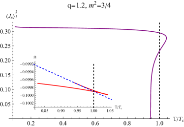
Figure 1: Left plot: The second-order phase transition occurs as the temperature falls below the critical value. The inset plot illustrates the scaling behavior of the condensate $\langle J_{x}\rangle$. Right plot: The first-order phase transition occurs when the temperature falls below the critical temperature, which represents by the black dashed line. The inset plot illustrates the effective free energy density $\Omega$ versus the temperature $T/T_{c}$, revealing that the superconducting phase is thermodynamically favored.

This holographic p-wave superconductor model can exhibit zeroth-order, first-order, and second-order phase transitions depending on the values of $m$ and $q$. For example, a second-order phase transition can occur at $q=1.5$, $m^{2}=3/4$ with a critical temperature of $T_{c}\approx 0.01791$. In Fig. 1, we demonstrate the relationship between the condensate $\langle J_{x}\rangle^{2/5}$ and temperature by plotting the scaling relationship,

$$\delta(\langle J_{x}\rangle)\sim\left(1-\frac{T}{T_{c}}\right)^{\alpha_{c}}.$$ (6)

Theoretical calculations predict that the critical exponent is $\alpha=1/2$ Cai:2013aca . Our numerical results also indicate that $\alpha_{c}\approx 0.500106$.

A first-order phase transition can occur at $q=1.2$ and $m^{2}=3/4$ with a critical temperature of $T_{c}\approx 0.003382$. To better visualize the phase structure, we plot the effective free energy density (as shown in Fig.1). The effective free energy density is defined as $\tilde{\Omega}=M-Ts$, where $T$ is the Hawking temperature, $s$ is the entropy density, and $M$ is the mass density of the black brane Liu:2021rks . The mass density of the black brane can be obtained by using the AdS asymptotic behavior of $g_{tt}$ in our ansatz,

$$\frac{(1-z)U(z)\left(-\frac{1}{4}\mu^{2}z^{3}+z^{2}+z+1\right)}{z^{2}}\sim\frac{1}{z^{2}}+Mz+Qz^{2}+\cdots.$$ (7)

The free energy of the superconducting phase is lower than the normal phase when the temperature drops below the critical temperature $T_{c}$. As a result, the system will abruptly transition from the normal phase to the superconducting phase.

To more thoroughly understand the behavior of p-wave superconductivity, we present the phase diagram in Fig. 2. The phase diagram is constructed by identifying the critical points, which can be found by examining the emergence of condensation as a perturbation near these points. The linearized equations of motion can be transformed into an eigenvalue problem that we solve using numerical methods

$$\frac{1}{32\mu^{2}(z-1)z^{2}}(\mu^{2}z^{3}-4z^{2}-4z -4)(2z^{2}(z^{2}(\mu^{2}(4z-3)-12)\rho_{x}^{\prime}(z)+$$ (8)

$$\left(\mu^{2}z^{4}-\left(\mu^{2}+4\right)z^{3}+4\right) \rho_{x}^{\prime\prime}(z))-6\rho_{x}(z))=-q^{2}\rho_{x}(z).$$

By analyzing the eigenvalues, we can determine the upper or lower bounds of the critical points, which correspond to the boundaries of the different phases in the diagram.

Figure 2: The phase diagram of holographic p-wave superconductor model with positive $m^{2}$. The solid lines are the critical points.

II.3 The holographic quantum information

Quantum entanglement is a fundamental characteristic of quantum systems. EE is a well-known measure of entanglement, which quantifies the correlation between a subsystem and its complement for pure states. It is defined in terms of the reduced density matrix $\rho_{A}$ Eisert:2008ur ,

$$S_{A}(|\psi\rangle)=-\text{Tr}[\rho_{A}\text{log}(\rho_{A})],\qquad\rho_{A}=\text{Tr}_{B}(|\psi\rangle\langle\psi|).$$ (9)

The HEE was proposed to be dual to the area of the minimum surface in the gravitational system Nishioka:2009un . In this paper, we consider the HEE of the configuration with an infinitely long strip along the $y$-axis (see Fig. 3). HEE typically diverges due to the asymptotic AdS boundary. The regulation is implemented by subtracting the divergent term from the HEE. It should be noted that HEE is not suitable for describing the mixed-state entanglement. For example, EE of the quantum system characterized by the direct product state $\mathcal{H}_{A}\otimes\mathcal{H}_{B}$ is not equal to zero, but the entanglement of the subsystems is vanishing. This is because EE contains both quantum and classical correlation. Therefore, as the dual of EE, HEE is also affected by thermodynamic entropy in mixed-state systems Ling:2015dma ; Ling:2016wyr .

Figure 3: Left plot: the minimum surface for a subsystem (red region). Right plot: the minimum cross-section (green surface) of the entanglement wedge.

To better solve the problem of mixed-state entanglement measurement, numerous novel entanglement measures have been proposed. One popular measure is mutual information (MI), which quantifies the correlation between two subsystems $A$ and $C$ that are separated by a subsystem $B$. According to the definition of MI, it is calculated as chuang:2002 ; Hayden:2011ag ,

$$I(a:c)=S(a)+S(c)-\text{min}(S(a\cup c)),$$ (10)

where $S(x)$ denotes the entanglement entropy of subsystem $x$. Unlike entanglement entropy, MI for direct product states $\mathcal{H}_{A}\otimes\mathcal{H}_{B}$ is always zero, making it a more appropriate measure for mixed-state entanglement. In the holographic context, the dual of MI is the difference in area between red (disconnected configuration) and blue surfaces (connected configuration), as shown in Fig. 4. As the subsystem $A,\,C$ becomes smaller or when the separation $B$ becomes larger, MI decreases and eventually reaches zero, indicating a disentangling phase transition. However, MI has some limitations as a mixed-state entanglement measure as it is directly related to entanglement entropy and can be dominated by it in some cases Huang:2019zph . Therefore, it is important to explore other mixed-state entanglement measures.

Recently, the minimum cross-section of the entanglement wedge (EWCS) is proposed as a novel holographic mixed-state entanglement measure Takayanagi:2017knl . EWCS is considered to be the duality of reflected entropy, logarithmic negativity, and odd entropy. The definition of EWCS is as follows,

$$E_{w}(\rho_{AB})=\underset{\Sigma_{AB}}{\text{min}}\left(\frac{\text{Area}(\Sigma_{AB})}{4G_{N}}\right).$$ (11)

Figure 4: The illustration of the holographic mutual information.

Fig. 3 is an illustration of EWCS in a bipartite system $a\cup c$ divided by $b$. The area bounded by the minimum surface of the disconnected configuration is known as the entanglement wedge. It is important to note that entanglement between subsystems only exists when the total correlation is not zero, which means the MI does not vanish.

Although EWCS plays a significant role in measuring the entanglement of mixed-state systems, it is still challenging to solve it Liu:2019qje . First, it is hard to solve the highly nonlinear EOM of the minimum surface. Second, the minimum cross-section is obtained by scanning a two-dimensional parameter space, which is a hard task. Last but not least, the coordinate singularity close to the AdS boundary with the asymptotic AdS can hinder numerical precision. We have proposed an efficient algorithm for solving EWCS based on the requirement that the minimum cross-section is locally orthogonal to the boundaries of the entanglement wedge Liu:2020blk . Fig. 5 shows the illustration of the key concept for our numerical algorithm. We consider EWCS of the infinite strip along the $y$-direction in a homogeneous background

$$ds^{2}=g_{tt}dt^{2}+g_{zz}dz^{2}+g_{xx}dx^{2}+g_{yy}dy^{2}.$$ (12)

The minimum surfaces of the connected configuration can be represented as $C_{1}(\theta_{1})$ and $C_{2}(\theta_{2})$. The minimum surfaces intersect with the cross-section at points $p_{1}$ and $p_{2}$, and the area of this local minimum surface (the red curve in Fig. 5) is,

$$A=\int_{C_{p_{1},p_{2}}}\sqrt{g_{xx}g_{yy}x^{\prime}(z)^{2}+g_{zz}g_{yy}}dz.$$ (13)

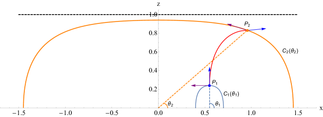
Figure 5: The illustration of the numerical algorithm for EWCS.

Variating (13), we obtain the EOM determining the local minimum surface,

$$x^{\prime}(z)^{3}\left(\frac{g_{xx}g_{yy}^{\prime}}{2g_{yy}g_{zz}}+\frac{g_{xx}^{\prime}}{2g_{zz}}\right)+x^{\prime}(z)\left(\frac{g_{xx}^{\prime}}{g_{xx}}+\frac{g_{yy}^{\prime}}{2g_{yy}}-\frac{g_{zz}^{\prime}}{2g_{zz}}\right)+x^{\prime\prime}(z)=0.$$ (14)

Remind that the global minimum cross-section is locally orthogonal to the entanglement wedge, which implies that

$$\left\langle\frac{\partial}{\partial_{z}},\frac{\partial}{\partial\theta_{1}}\right\rangle_{p_{1}}=0,\quad\left\langle\frac{\partial}{\partial_{z}},\frac{\partial}{\partial\theta_{2}}\right\rangle_{p_{2}}=0$$ (15)

where $\langle\cdot,\cdot\rangle$ represents the vector product with metric $g_{\mu\nu}$. We can normalize the orthogonal relation,

$$Q_{1}(\theta_{1},\theta_{2})\equiv\left.\frac{\langle\frac{\partial}{\partial z},\frac{\partial}{\partial\theta_{1}}\rangle}{\sqrt{\langle\frac{\partial}{\partial z},\frac{\partial}{\partial z}\rangle\langle\frac{\partial}{\partial\theta_{1}},\frac{\partial}{\partial\theta_{1}}\rangle}}\right|_{p_{1}}=0,\quad Q_{2}(\theta_{1},\theta_{2})\equiv\left.\frac{\langle\frac{\partial}{\partial z},\frac{\partial}{\partial\theta_{1}}\rangle}{\sqrt{\langle\frac{\partial}{\partial z},\frac{\partial}{\partial z}\rangle\langle\frac{\partial}{\partial\theta_{2}},\frac{\partial}{\partial\theta_{2}}\rangle}}\right|_{p_{2}}=0.$$ (16)

Finding the cross-section located at the minimum surface at $(\theta_{1},\theta_{2})$ where (16) is satisfied, we obtain the minimum cross-section. To this end, we adopt the Newton-Raphson method to locate the endpoints satisfying the local perpendicular conditions. Based on the above techniques, we can study the relationship between the holographic p-wave superconductor and the EWCS Liu:2020blk .

III The computation of the holographic quantum information

III.1 The holographic entanglement entropy and mutual information

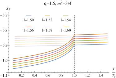
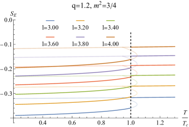
Figure 6: The holographic entanglement entropy $S_{E}$ vs temperature $T/T_{c}$ with various strip width $l$. The critical point is indicated by the black dashed line. The stable and metastable states are depicted by solid and transparent lines, respectively. Left plot: The second-order phase transition at $T_{c}\approx 0.01791$. Right plot: The first-order phase transition at $T_{c}\approx 0.003382$.

In Fig. 6, we show the relationship between the HEE and temperature $T/T_{c}$ during second-order and first-order phase transitions. For $q=1.5$ and $m^{2}=3/4$, where the second-order phase transition occurs, the HEE increases with increasing temperature. For $q=1.2$ and $m^{2}=3/4$, where the first-order phase transition occurs, the HEE jumps abruptly when crossing the critical point. To understand this behavior, we can examine the relationship between HEE and thermodynamic entropy, as when the configuration is large or the temperature is high enough, the minimum surface will approach the horizon of the black brane and HEE will primarily be determined by thermodynamic entropy. Therefore, we will next analyze the thermodynamic entropy behavior of the black brane to better understand the behavior of HEE Ling:2016wyr ; Ling:2015dma .

The entropy density is given by,

$$\tilde{s}=\frac{2\pi A}{\kappa^{2}}=\frac{2\pi\sqrt{V_{1}(z)V_{2}(z)}}{\kappa^{2}}\hat{V},$$ (17)

where $A$ is the area of the horizon and $\hat{V}=\int dxdy$ is the corresponding area of the region in the dual field theory Nguyen:2015wfa . Dividing the entropy by the area $\hat{V}$ and $\mu^{2}$, we have the dimensionless entropy density $s=\frac{\kappa^{2}\tilde{s}}{2\pi\hat{V}\mu^{2}}$. The plot of the entropy density near the critical point can be seen in Fig. 7. The above phenomena show that both HEE and entropy density can detect the critical behavior of the holographic p-wave superconducting phase transitions. Similar phenomena of the HEE in the superconducting phase transition can see in Liu:2020blk ; Cai:2012sk ; Peng:2015yaa ; Peng:2014ira .

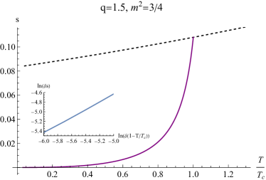
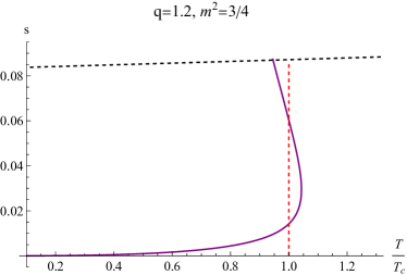
Figure 7: The entropy density $s$ vs temperature $T/T_{c}$. The black dashed line represents the entropy density of the normal phase. The entropy density of the superconducting phase is represented by the purple line. Left plot: The second-order phase transition of holographic p-wave superconductor model. The inset plot depicts the logarithm between $s$ and $1-\frac{T}{T_{c}}$. Right plot: The first-order phase transition of holographic p-wave superconductor model. The critical temperature is indicated by the red dashed line.

MI is one of the mixed-state entanglement measures that can extract the total correlation of the systems. Since MI is directly defined by HEE (see (10)), it also can diagnose the phase transition. Moreover, a disentangling phase transition occurs when MI is zero and entanglement exists only when MI is greater than zero. Fig. 8 illustrates the behavior of the disentangling phase transition for various configurations. However, in certain cases, MI is determined by the thermodynamic entropy Liu:2020blk ; Liu:2021rks ; Huang:2019zph . Therefore, it is necessary to investigate other mixed-state entanglement measures.

Figure 8: The critical configuration for disentangling phase transition. The critical temperature is indicated by the black dashed line. The solid and translucent lines represent stable and metastable states. Left plot: When $b$ is above the $b_{c}$, the disentangling phase transition occurs. Right plot: When $c$ is below $c_{c}$, the disentangling phase transition occurs.

III.2 The minimum entanglement wedge cross section

We begin by examining the EWCS during a second-order phase transition. Fig. 9 shows that EWCS can diagnose the critical behavior of holographic p-wave superconducting phase transitions. At the critical point of a second-order phase transition, EWCS is continuous, but its first derivative is discontinuous. In the superconducting phase, EWCS always decreases with increasing temperature. However, we find that the EWCS in the normal phase is configuration-dependent. In large configurations, it behaves similarly to the HEE, showing a monotonically increasing trend with temperature. In contrast, for small configurations, the EWCS of the normal phase exhibits a monotonically decreasing trend with temperature, opposite to the behavior of the HEE.

Figure 9: The EWCS $E_{w}$ vs the temperature $T/T_{c}$. The inset graph depicts $\partial_{T}E_{w}$. The black dashed line depicts the critical temperature. Left plot: The $\partial_{T}E_{w}$ of the normal phase is greater than zero when $a=2$ and $b=0.5$. Right plot: The $\partial_{T}E_{w}$ of the normal phase is less than zero when $a=1$ and $b=0.2$.

Next, we investigate the behavior of the EWCS during a first-order phase transition. Fig. 10 illustrates EWCS behavior during this phase transition, with the inset plot showing the derivative of EWCS with respect to temperature ($\partial_{T}E_{w}$) versus temperature $T$. The inset plot illustrates that in normal phase the EWCS decreases with increasing temperature. Unlike the HEE, the EWCS of the superconducting phase always decreases with temperature. When the temperature falls below a critical point, EWCS abruptly jumps from the normal phase to the superconducting phase, this sudden change in EWCS suggests that it can capture the first-order phase transition, similar to the HEE and MI.

In addition to diagnosing the critical points, it is also important to investigate the scaling behavior of the holographic quantum information. Next, we analyze the critical behavior of the quantum information-related quantities during the p-wave superconductivity phase transitions.

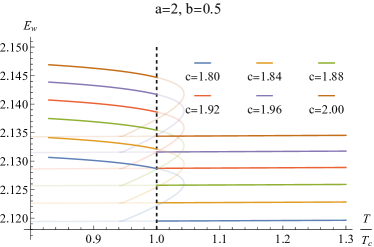
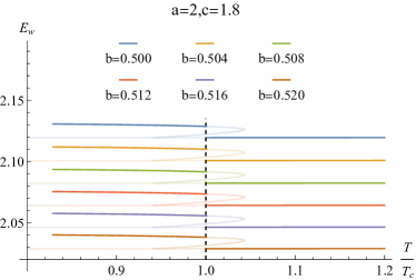
Figure 10: The EWCS $E_{w}$ versus the temperature $T/T_{c}$ in the first-order phase transition. The dashed black line represents the critical temperature when $T_{c}\approx 0.003382$. The translucent line represents the metastable state, whereas the solid line represents the stable state. Left plot: We set $a=2$ and $b=0.5$ with varying $c$ values. Right plot: We set $a=2$ and $c=1.8$ while varying $b$ values.

IV The Scaling behavior of the quantum information

As the critical point marks the bifurcation point between the normal and superconducting phases, to study the critical behavior, we compare the quantum information quantities of the normal phase to those of the superconducting phase by subtracting the former from the latter,

$$\delta S_{E}=S^{\text{cond}}_{E}-S^{\text{normal}}_{E},\quad\delta E_{w}=E^{\text{cond}}_{w}-E^{\text{normal}}_{w}.$$ (18)

We propose the following critical behaviors for the HEE and EWCS,

$$\delta S\sim\left(1-\frac{T}{T_{c}}\right)^{\alpha_{\text{HEE}}},\quad\delta E_{w}\sim\left(1-\frac{T}{T_{c}}\right)^{\alpha_{\text{EWCS}}},$$ (19)

where $\alpha_{\text{HEE}}$ and $\alpha_{\text{EWCS}}$ are the critical exponent of the HEE and EWCS, respectively.

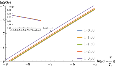
Figure 11: The scaling behavior of HEE and EWCS. The inset plot shows the slope of the holographic quantum information. Left plot: $\text{ln}(\delta S_{E})$ versus $\text{ln}(\delta(1-\frac{T}{Tc}))$ with different width of $l$. Right plot: we set $a=2$ and $b=0.5$ and $\text{ln}(\delta E_{w})$ versus $\text{ln}(\delta(1-\frac{T}{T_{c}}))$ with different values of $c$.

We plot the critical scaling behavior in Fig. 11, from which we find that both EWCS and HEE exhibit excellent scaling behavior near the critical point. More importantly, they both have the same critical exponent,

$$\alpha_{\text{HEE}}\approx\alpha_{\text{EWCS}}\approx 1.$$ (20)

It is important to note that the vector field $\rho_{\mu}$ is always zero at temperatures higher than the critical temperature. At temperatures slightly below the critical point, the condensate vacuum expectation value of $\langle J_{x}\rangle$ is small and can be analyzed using perturbation theory. We can expand the vector field $\rho_{\mu}$ and the metric function near the critical point as Zeng:2010zn ; Pan:2012jf ; Ammon:2009xh ,

$$\rho_{x} =\epsilon\rho^{(1)}+\epsilon^{3}\rho^{(3)}+\epsilon^{5}\rho^{(5)}+\cdots,$$ (21)

$$U =1+\epsilon^{2}U^{(1)}+\epsilon^{4}U^{(4)}+\cdots,$$

$$V_{1} =1+\epsilon^{2}V_{1}^{(1)}+\epsilon^{4}V_{1}^{(4)}+\cdots.$$

From (21), we can deduce that the critical exponent of the metric function $U$, $V_{1}$, is twice that of the condensate $\langle J_{x}\rangle$. This can be understood by noting that holographic quantum information is represented by geometric objects that depend only on the metric. Their critical exponent can be written as,

$$\delta(S_{E})\sim\delta(E_{w})\sim\delta(\langle J_{x}\rangle)^{2}\sim\left(1-\frac{T}{T_{c}}\right)^{2\alpha_{c}}.$$ (22)

Therefore, the theoretical critical exponent of holographic quantum information should be twice that of the condensate $\langle J_{x}\rangle$,

$$\alpha_{\text{HEE}}=\alpha_{\text{EWCS}}=2\alpha_{c}.$$ (23)

Although EWCS and HEE have the same critical exponent in the critical region, they do not tend to the scaling law at the same rate in the critical region. To better investigate this phenomenon near the critical point, we define the quasi-critical exponent (QCE) as

$$\alpha\equiv\frac{d\ln(\delta S)}{d\ln\left(1-\frac{T}{T_{c}}\right)}.$$ (24)

QCE is a function of $\ln\left(1-\frac{T}{T_{c}}\right)$. Apparently, the QCE $\alpha$ behavior along $\ln\left(1-\frac{T}{T_{c}}\right)$ can measure the extent to which a wide range of $S$ can converge to the scaling law.

We show the QCE of HEE and EWCS in Fig. 12.

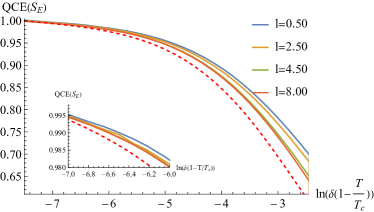
Figure 12: The QCE of the HEE and EWCS. The red dashed line represents the twice QCE of the condensate $\langle J_{x}\rangle$. Left plot: The QCE of the HEE near the critical points. Right plot: The QCE of the EWCS near the critical points, when we fix the $a=2$ and $c=1.5$.

From the left plot of Fig. 12 we find that the width $l$ has an impact on the scaling behavior of HEE. As the width $l$ increases, the scaling behavior of HEE is closer to the theoretical scaling behavior. As the temperature moves away from the critical point or the width $l$ decreases, however, the scaling behavior of the HEE begins to deviate from the theoretical result.

The QCE of EWCS is depicted in the right plot of Fig. 12. Comparing the left plot and the right plot of Fig. 12, EWCS converges to the theoretical scaling law over a broader range. As the separation $b$ decreases, the scaling behavior of EWCS becomes close to the theoretical results. This behavior suggests that EWCS, as a measure for mixed-state entanglement, can more accurately describe the scaling behavior during superconductivity phase transitions than HEE.

V The growth rate of the holographic quantum information

Several important inequalities involving the EWCS have been proposed in the literature Umemoto:2018jpc ; Li:2022wim ; Bao:2017nhh , such as the inequality $E_{w}(\rho_{AC})\geq\frac{1}{2}I(A,c)$, which states that the EWCS cannot be smaller than half of the MI. These inequalities are crucial in the study of mixed-state entanglement measures, particularly in testing the validity of holographic duals of certain quantum information. In this paper, we find a new inequality behavior of EWCS and MI related to the superconductivity phase transition: near the phase transition point, the relative growth rate of MI along the temperature axis is always greater than that of EWCS.

Figure 13: The relative value of MI and EWCS near the critical point. The dashed lines represent $\tilde{I}$ and the solid lines represent $\tilde{E}_{w}$. The inset plot is the slope of $\tilde{I}$ and $\tilde{E}_{w}$. Left plot: We fix the subsystems $a=c=2$ and change the separation $b$. Right plot: We fix the separation $b=0.1$ and change the subsystem $a$ and $c$.

When the temperature drops below the critical temperature, the EWCS and the MI of the superconducting phases are always larger than those of the normal phases. To take a closer look at the relationship between the EWCS and the MI, we define the relative values of the MI and the EWCS,

$$\tilde{E}_{w}=\frac{E_{w,\text{cond}}}{E_{w,\text{norm}}},\quad\tilde{I}=\frac{I_{\text{cond}}}{I_{\text{norm}}}.$$ (25)

With this definition, $\tilde{E}_{w}$ and $\tilde{I}$ are fixed at $1$ at the critical point. In Fig. 13, we depict the relationship between the $\tilde{I}$ and $\tilde{E}_{w}$. Contrary to the inequality Umemoto:2018jpc ; Li:2022wim ; Bao:2017nhh , the relative MI is always larger than the relative values of EWCS in the critical region. To describe this relationship quantitatively, we examine the fact that,

$$\delta(Q)\simeq A(Q)\left(1-\frac{T}{T_{c}}\right)^{\alpha},$$ (26)

where $Q$ stands for any physical quantity possessing critical behaviors. From (26) we find that,

$$\tilde{E}_{w}=1+A(\tilde{E}_{w})\left(1-\frac{T}{T_{c}}\right)^{\alpha},\quad\tilde{I}=1+A(\tilde{I})\left(1-\frac{T}{T_{c}}\right)^{\alpha}.$$ (27)

Accordingly, it can be seen that $A$ actually measures the increasing phenomenon of holographic quantum information in Fig. 12, and hence we call $A$ the growth rate. We work out $A(\tilde{E}_{w})$ and $A(\tilde{I})$ for several different configurations and list them in Table 1. From these numerical results we conclude a new inequality between the EWCS and MI growth rates near the critical point,

$$A(\tilde{I})>A(\tilde{E}_{w}).$$ (28)

The growth rate of MI is always greater than that of EWCS near the critical point. Furthermore, the difference between the growth rates of EWCS and MI increases as the subsystem separation $b$ increases. Near the critical point, the entanglement of the system changes rapidly, and MI is more sensitive to these changes than EWCS. This tendency could be attributed to MI’s ability to capture the total correlation of the system, which exceeds the information captured by EWCS. Additionally, we have examined this inequality in other models of thermal phase transitions, including the holographic s-wave superconductor model, and propose that this inequality may be universal in thermal phase transitions.

Table 1: The growth rate $A(\tilde{E}_{w})$ and $A(\tilde{I})$ at different configurations.

Configuration	A($\tilde{E}_{w}$)	A($\tilde{I}$)
$a=c=2$, $b=0.20$	0.0426	0.0741
$a=c=2$, $b=0.47$	0.1162	0.2947
$a=c=2$, $b=0.73$	0.2094	0.9855
$a=c=2$, $b=1.00$	0.3212	10.8712
$a=0.8$, $b=0.2$, $c=0.4$	0.00218	0.00525
$a=0.8$, $b=0.2$, $c=0.8$	0.00520	0.00803
$a=0.8$, $b=0.2$, $c=1.2$	0.00862	0.01336
$a=0.8$, $b=0.2$, $c=1.6$	0.01209	0.01975
$a=0.5$, $b=0.2$, $c=0.4$	0.00116	0.00364
$a=1.0$, $b=0.2$, $c=0.9$	0.00794	0.01182
$a=1.5$, $b=0.2$, $c=1.4$	0.02016	0.03120
$a=3.0$, $b=0.2$, $c=2.9$	0.06042	0.11959

VI Discussion

In this study, we investigate mixed-state entanglement measures, including HEE, MI and EWCS, in a holographic p-wave superconductor model. The model exhibits both second and first-order phase transitions when varying system parameters. We find that HEE and EWCS can accurately diagnose the critical behavior of these phase transitions. Additionally, we observe that the behavior of HEE is related to thermodynamic entropy as the subsystem configuration increases. However, as a mixed-state entanglement measure, EWCS exhibits the opposite behavior from HEE in the superconducting phase. Specifically, HEE always increases with temperature, whereas EWCS in the superconducting state decreases with temperature. In the case of first-order phase transitions, the holographic quantum information experiences sudden changes. However, the EWCS behavior in the normal phase is dependent on the subsystem configuration. This behavior demonstrates that EWCS can not only detect phase transitions but also capture more information than HEE.

In addition to diagnosing phase transitions, we also examine the scaling behaviors of the condensate and the holographic quantum information. Through analyzing the scaling behavior of various holographic quantum information measures, we find that HEE and EWCS not only detect the critical point but also exhibit scaling behaviors. We show both numerically and analytically that the critical exponent of holographic quantum information is twice that of the condensate. Furthermore, we observe that compared to HEE, EWCS provides a more sensitive characterization of the scaling behavior, making it more suitable as a measure for mixed-state entanglement in superconductivity phase transitions. Additionally, we propose a novel inequality for EWCS and MI in phase transitions and provide numerical evidence for this result. The relative growth rate of MI is always larger than that of EWCS near the critical point.

Next, we point out several directions worth further investigation. The investigation of topological and quantum phase transitions is an important area of research in condensed matter theory Donos:2013eha ; Landsteiner:2015pdh ; Ling:2016dck ; Baggioli:2018afg ; Baggioli:2020cld . In addition, the relationship between HEE and quantum phase transitions has been studied under holographic framework in previous works Ling:2016wyr ; Ling:2015dma . Further research into the mixed-state entanglement in quantum phase transitions and topological quantum phase transitions is therefore desirable. Additionally, it would be interesting to test the inequality (28) in other thermal phase transition models, such as the $d$-wave superconductivity model and the massive gravity model. We are working on these directions.

References

- (1) J. Eisert, “Entanglement in quantum information theory,” arXiv preprint quant-ph/0610253, 2006.
- (2) A. Osterloh, L. Amico, G. Falci, R. Fazio, “Scaling of Entanglement close to a Quantum Phase Transitions” Nature 416, 608 (2002) [arXiv:0202029 [quant-ph]]
- (3) L. Amico, R. Fazio, A. Osterloh and V. Vedral, “Entanglement in many-body systems” Rev.Mod.Phys. 80, 517 (2008) [arXiv:0703044 [quant-ph]]
- (4) Levin, Michael, and Xiao-Gang Wen. “Detecting topological order in a ground state wave function”. Physical review letters 96.11 (2006): 110405.
- (5) Kitaev, Alexei, and John Preskill. “Topological entanglement entropy”. Physical review letters 96.11 (2006): 110404.
- (6) G. Vidal and R. F. Werner, “Computable measure of entanglement,” Phys. Rev. A 65 (2002), 032314 doi:10.1103/PhysRevA.65.032314 [arXiv:quant-ph/0102117 [quant-ph]].
- (7) R. Horodecki, P. Horodecki, M. Horodecki and K. Horodecki, “Quantum entanglement,” Rev. Mod. Phys. 81 (2009), 865-942 doi:10.1103/RevModPhys.81.865 [arXiv:quant-ph/0702225 [quant-ph]].
- (8) G. ’t Hooft, “Dimensional reduction in quantum gravity,” Salamfest 1993:0284-296
- (9) L. Susskind, “The World as a hologram” J. Math. Phys. 36, 6377 (1995)
- (10) J. M. Maldacena, “The Large N limit of superconformal field theories and supergravity,” Int. J. Theor. Phys. 38, 1113 (1999) [Adv. Theor. Math. Phys. 2, 231 (1998)]
- (11) E. Witten, “Anti-de Sitter space and holography,” Adv. Theor. Math. Phys. 2, 253 (1998)
- (12) S. A. Hartnoll, A. Lucas and S. Sachdev, “Holographic quantum matter,” [arXiv:1612.07324 [hep-th]].
- (13) S. Ryu and T. Takayanagi, “Holographic derivation of entanglement entropy from AdS/CFT,” Phys. Rev. Lett. 96, 181602 (2006)
- (14) R. G. Cai, S. He, L. Li and Y. L. Zhang, “Holographic Entanglement Entropy on P-wave Superconductor Phase Transition,” JHEP 07 (2012), 027 doi:10.1007/JHEP07(2012)027 [arXiv:1204.5962 [hep-th]].
- (15) Y. Peng and Q. Pan, “Holographic entanglement entropy in general holographic superconductor models,” JHEP 06 (2014), 011 doi:10.1007/JHEP06(2014)011 [arXiv:1404.1659 [hep-th]].
- (16) Y. Peng, “Holographic entanglement entropy in superconductor phase transition with dark matter sector,” Phys. Lett. B 750 (2015), 420-426 doi:10.1016/j.physletb.2015.09.052 [arXiv:1507.07399 [hep-th]].
- (17) X. X. Zeng, H. Zhang and L. F. Li, “Phase transition of holographic entanglement entropy in massive gravity,” Phys. Lett. B 756 (2016), 170-179 doi:10.1016/j.physletb.2016.03.013 [arXiv:1511.00383 [gr-qc]].
- (18) K. Umemoto and T. Takayanagi, “Entanglement of purification through holographic duality,” Nature Phys. 14, no. 6, 573 (2018)
- (19) K. Umemoto and Y. Zhou, “Entanglement of Purification for Multipartite States and its Holographic Dual,” JHEP 1810, 152 (2018)
- (20) S. Dutta and T. Faulkner, “A canonical purification for the entanglement wedge cross-section,” JHEP 03 (2021), 178 doi:10.1007/JHEP03(2021)178 [arXiv:1905.00577 [hep-th]].
- (21) J. Kudler-Flam and S. Ryu, “Entanglement negativity and minimal entanglement wedge cross sections in holographic theories,” Phys. Rev. D 99 (2019) no.10, 106014 doi:10.1103/PhysRevD.99.106014 [arXiv:1808.00446 [hep-th]].
- (22) N. Jokela and A. Pönni, “Notes on entanglement wedge cross sections,” JHEP 07 (2019), 087 doi:10.1007/JHEP07(2019)087 [arXiv:1904.09582 [hep-th]].
- (23) K. Babaei Velni, M. R. Mohammadi Mozaffar and M. H. Vahidinia, JHEP 05 (2019), 200 doi:10.1007/JHEP05(2019)200 [arXiv:1903.08490 [hep-th]].
- (24) M. J. Vasli, M. R. Mohammadi Mozaffar, K. Babaei Velni and M. Sahraei, “Holographic study of reflected entropy in anisotropic theories,” Phys. Rev. D 107, no.2, 026012 (2023) doi:10.1103/PhysRevD.107.026012 [arXiv:2207.14169 [hep-th]].
- (25) H. A. Camargo, P. Nandy, Q. Wen and H. Zhong, “Balanced partial entanglement and mixed state correlations,” SciPost Phys. 12, no.4, 137 (2022) doi:10.21468/SciPostPhys.12.4.137 [arXiv:2201.13362 [hep-th]].
- (26) P. Liu, Y. Ling, C. Niu and J. P. Wu, “Entanglement of Purification in Holographic Systems,” arXiv:1902.02243 [hep-th].
- (27) Y. f. Huang, Z. j. Shi, C. Niu, C. y. Zhang and P. Liu, “Mixed State Entanglement for Holographic Axion Model,” Eur. Phys. J. C 80, no.5, 426 (2020) doi:10.1140/epjc/s10052-020-7921-y [arXiv:1911.10977 [hep-th]].
- (28) P. Liu and J. P. Wu, “Mixed state entanglement and thermal phase transitions,” Phys. Rev. D 104 (2021) no.4, 046017 doi:10.1103/PhysRevD.104.046017 [arXiv:2009.01529 [hep-th]].
- (29) C. Y. Chen, W. Xiong, C. Niu, C. Y. Zhang and P. Liu, “Entanglement wedge minimum cross-section for holographic aether gravity,” JHEP 08 (2022), 123 doi:10.1007/JHEP08(2022)123 [arXiv:2109.03733 [hep-th]].
- (30) Y. Z. Li, C. Y. Zhang and X. M. Kuang, “Entanglement wedge cross-section with Gauss-Bonnet corrections and thermal quench,” Sci. China Phys. Mech. Astron. 64 (2021) no.12, 120413 [arXiv:2102.12171 [hep-th]].
- (31) A. R. Chowdhury, A. Saha and S. Gangopadhyay, “Entanglement wedge cross-section for noncommutative Yang-Mills theory,” JHEP 02, 192 (2022) doi:10.1007/JHEP02(2022)192 [arXiv:2106.04562 [hep-th]].
- (32) M. Sahraei, M. J. Vasli, M. R. M. Mozaffar and K. B. Velni, “Entanglement wedge cross section in holographic excited states,” JHEP 08, 038 (2021) doi:10.1007/JHEP08(2021)038 [arXiv:2105.12476 [hep-th]].
- (33) A. Chowdhury Roy, A. Saha and S. Gangopadhyay, “Mixed state information theoretic measures in boosted black brane,” [arXiv:2204.08012 [hep-th]].
- (34) S. Maulik, “More on entanglement properties of spacetime with string excitations,” [arXiv:2209.05207 [hep-th]].
- (35) P. Jain and S. Mahapatra, “Mixed state entanglement measures as probe for confinement,” Phys. Rev. D 102, 126022 (2020) doi:10.1103/PhysRevD.102.126022 [arXiv:2010.07702 [hep-th]].
- (36) P. Jain, S. S. Jena and S. Mahapatra, “Holographic confining/deconfining gauge theories and entanglement measures with a magnetic field,” [arXiv:2209.15355 [hep-th]].
- (37) S. A. Hartnoll, C. P. Herzog and G. T. Horowitz, “Holographic Superconductors,” JHEP 12 (2008), 015 doi:10.1088/1126-6708/2008/12/015 [arXiv:0810.1563 [hep-th]].
- (38) G. T. Horowitz, “Introduction to Holographic Superconductors,” Lect. Notes Phys. 828 (2011), 313-347 doi:10.1007/978-3-642-04864-7_10 [arXiv:1002.1722 [hep-th]].
- (39) S. A. Hartnoll, C. P. Herzog and G. T. Horowitz, “Building a Holographic Superconductor,” Phys. Rev. Lett. 101 (2008), 031601 doi:10.1103/PhysRevLett.101.031601 [arXiv:0803.3295 [hep-th]].
- (40) Y. Ling, P. Liu, C. Niu, J. P. Wu and Z. Y. Xian, “Holographic Superconductor on Q-lattice,” JHEP 1502, 059 (2015)
- (41) M. Rogatko and K. I. Wysokinski, JHEP 12, 041 (2015) doi:10.1007/JHEP12(2015)041 [arXiv:1510.06137 [hep-th]].
- (42) R. E. Arias and I. S. Landea, “Backreacting p-wave Superconductors,” JHEP 01, 157 (2013) doi:10.1007/JHEP01(2013)157 [arXiv:1210.6823 [hep-th]].
- (43) R. G. Cai, L. Li, L. F. Li and R. Q. Yang, “Introduction to Holographic Superconductor Models,” Sci. China Phys. Mech. Astron. 58 (2015) no.6, 060401 doi:10.1007/s11433-015-5676-5 [arXiv:1502.00437 [hep-th]].
- (44) M. Rogatko and K. I. Wysokinski, “P-wave holographic superconductor/insulator phase transitions affected by dark matter sector,” JHEP 03, 215 (2016) doi:10.1007/JHEP03(2016)215 [arXiv:1508.02869 [hep-th]].
- (45) T. Albash and C. V. Johnson, “Holographic Studies of Entanglement Entropy in Superconductors,” JHEP 05 (2012), 079 doi:10.1007/JHEP05(2012)079 [arXiv:1202.2605 [hep-th]].
- (46) H. S. Jeong, K. Y. Kim and Y. W. Sun, “Holographic entanglement density for spontaneous symmetry breaking,” JHEP 06, 078 (2022) doi:10.1007/JHEP06(2022)078 [arXiv:2203.07612 [hep-th]].
- (47) R. G. Cai, L. Li and L. F. Li, “A Holographic P-wave Superconductor Model,” JHEP 01 (2014), 032 doi:10.1007/JHEP01(2014)032 [arXiv:1309.4877 [hep-th]].
- (48) R. G. Cai, L. Li, L. F. Li and R. Q. Yang, “Towards Complete Phase Diagrams of a Holographic P-wave Superconductor Model,” JHEP 04 (2014), 016 doi:10.1007/JHEP04(2014)016 [arXiv:1401.3974 [gr-qc]].
- (49) P. Liu, C. Niu, Z. J. Shi and C. Y. Zhang, “Entanglement wedge minimum cross-section in holographic massive gravity theory,” JHEP 08 (2021), 113 doi:10.1007/JHEP08(2021)113 [arXiv:2104.08070 [hep-th]].
- (50) J. Eisert, M. Cramer and M. B. Plenio, “Area laws for the entanglement entropy - a review,” Rev. Mod. Phys. 82 (2010), 277-306 doi:10.1103/RevModPhys.82.277 [arXiv:0808.3773 [quant-ph]].
- (51) T. Nishioka, S. Ryu and T. Takayanagi, “Holographic Entanglement Entropy: An Overview,” J. Phys. A 42 (2009), 504008 doi:10.1088/1751-8113/42/50/504008 [arXiv:0905.0932 [hep-th]].
- (52) Y. Ling, P. Liu, C. Niu, J. P. Wu and Z. Y. Xian, “Holographic Entanglement Entropy Close to Quantum Phase Transitions,” JHEP 1604, 114 (2016)
- (53) Y. Ling, P. Liu and J. P. Wu, “Characterization of Quantum Phase Transition using Holographic Entanglement Entropy,” Phys. Rev. D 93, no. 12, 126004 (2016)
- (54) Nielsen M A, Chuang I. “Quantum computation and quantum information” [J]. 2002.
- (55) P. Hayden, M. Headrick and A. Maloney, “Holographic Mutual Information is Monogamous,” Phys. Rev. D 87 (2013) no.4, 046003 doi:10.1103/PhysRevD.87.046003 [arXiv:1107.2940 [hep-th]].
- (56) P. H. Nguyen, “An equal area law for holographic entanglement entropy of the AdS-RN black hole,” JHEP 12 (2015), 139 doi:10.1007/JHEP12(2015)139 [arXiv:1508.01955 [hep-th]].
- (57) R. G. Cai, S. He, L. Li and Y. L. Zhang, “Holographic Entanglement Entropy in Insulator/Superconductor Transition,” JHEP 07 (2012), 088 doi:10.1007/JHEP07(2012)088 [arXiv:1203.6620 [hep-th]].
- (58) H. B. Zeng, X. Gao, Y. Jiang and H. S. Zong, “Analytical Computation of Critical Exponents in Several Holographic Superconductors,” JHEP 05 (2011), 002 doi:10.1007/JHEP05(2011)002 [arXiv:1012.5564 [hep-th]].
- (59) Q. Pan, J. Jing, B. Wang and S. Chen, “Analytical study on holographic superconductors with backreactions,” JHEP 06 (2012), 087 doi:10.1007/JHEP06(2012)087 [arXiv:1205.3543 [hep-th]].
- (60) M. Ammon, J. Erdmenger, V. Grass, P. Kerner and A. O’Bannon, “On Holographic p-wave Superfluids with Back-reaction,” Phys. Lett. B 686 (2010), 192-198 doi:10.1016/j.physletb.2010.02.021 [arXiv:0912.3515 [hep-th]].
- (61) P. Li and Y. Ling, “Entanglement wedge cross section inequalities in AdS/BCFT,” Phys. Rev. D 106 (2022) no.8, 086021 doi:10.1103/PhysRevD.106.086021 [arXiv:2206.13417 [hep-th]].
- (62) N. Bao and I. F. Halpern, JHEP 03 (2018), 006 doi:10.1007/JHEP03(2018)006 [arXiv:1710.07643 [hep-th]].
- (63) A. Donos and J. P. Gauntlett, “Holographic Q-lattices,” JHEP 04 (2014), 040 doi:10.1007/JHEP04(2014)040 [arXiv:1311.3292 [hep-th]].
- (64) K. Landsteiner, Y. Liu and Y. W. Sun, “Quantum phase transition between a topological and a trivial semimetal from holography,” Phys. Rev. Lett. 116 (2016) no.8, 081602 doi:10.1103/PhysRevLett.116.081602 [arXiv:1511.05505 [hep-th]].
- (65) Y. Ling, P. Liu, J. P. Wu and Z. Zhou, “Holographic Metal-Insulator Transition in Higher Derivative Gravity,” Phys. Lett. B 766 (2017), 41-48 doi:10.1016/j.physletb.2016.12.051 [arXiv:1606.07866 [hep-th]].
- (66) M. Baggioli, B. Padhi, P. W. Phillips and C. Setty, “Conjecture on the Butterfly Velocity across a Quantum Phase Transition,” JHEP 07, 049 (2018) doi:10.1007/JHEP07(2018)049 [arXiv:1805.01470 [hep-th]].
- (67) M. Baggioli and D. Giataganas, “Detecting Topological Quantum Phase Transitions via the c-Function,” Phys. Rev. D 103, no.2, 026009 (2021) doi:10.1103/PhysRevD.103.026009 [arXiv:2007.07273 [hep-th]].