The fundamental solution of the master equation for a jump-diffusion Ornstein-Uhlenbeck process

Abstract.

An integro-differential equation for the probability density of the generalized stochastic Ornstein-Uhlenbeck process with jump diffusion is considered for a special case of the Laplacian distribution of jumps. It is shown that for a certain ratio between the intensity of jumps and the speed of reversion, the fundamental solution can be found explicitly, as a finite sum. Alternatively, the fundamental solution can be represented as converging power series. The properties of this solution are investigated. The fundamental solution makes it possible to obtain explicit formulas for the density at each instant of time, which is important, for example, for testing numerical methods.

1. Introduction

Models using stochastic dynamics have natural applications in various areas of physics, biology, and financial mathematics. In recent decades, it has become clear that many phenomena cannot be explained by adding only standard Wiener processes to deterministic models, it is necessary to consider models that take into account differently distributed jumps, that is, use non-Gaussian stochastic models. For example, let us mention some works where non-Gaussian models are used in physics of metals [11], [1], in the study of neural networks [24] and genome behavior [2], [16], in weather forecasting [25], and in financial mathematics [3].

Although models using non-Gaussian stochastic dynamics are quite diverse, their probability density necessarily obeys some generalized Kolmogorov-Fokker-Planck equation containing a non-local (integral) term. Such equations are sometimes called the Kolmogorov-Feller equations. There are many mathematical works that study the existence of density and its smoothness for various types of non-Gaussian processes, the properties of transition probability [20], [21], [10], [12], [19]. However, in practice, when solving such equations, one usually has to use numerical methods [8].

In this paper, we consider the simplest generalization of the Ornstein-Uhlenbeck process to the case of jump diffusion. Such processes have traditional applications to active particle dynamics [4], as well as to modeling of interest rates in financial mathematics [15].

Previously, it was known that the assumption of a connection between the force acting on the particle and the properties of the kernel of the jump process helps to construct an exact solution of the corresponding stationary Kolmogorov-Feller equation, that is, to study the large time density distribution [4], [22].

However, apparently, it was not noticed earlier that in some cases the assumption of a connection between the intensity of jumps and the speed of reversion allows one to obtain an explicit formula for the fundamental solution, and hence, to obtain an integral formula for the dynamics of an arbitrary initial density as a convolution. Moreover, for some initial densities (e.g. Gaussian or piecewise constant density), one can obtain an explicit formula describing the dynamics of the density at all times. This is valuable, in particular, for testing numerical algorithms.

The properties of fundamental solutions for integro-differential equations have been studied in previous works. For example, in [9] the asymptotics of the fundamental solution was constructed depending on the properties of the kernel of the process describing the jumps. It was also noted that in the case of pure jumps (without diffusion), the fundamental solution always contains a singular component.

In this paper, a fundamental solution of the Kolmogorov-Feller equation is constructed for the case of a Laplacian distribution of jumps. In the general case, the fundamental solution can be written as a series; however, with a countable number of dependencies between the return force and the intensity of the jump process, this series reduces to a finite sum. These exact formulas make it possible, in particular, to study in detail the smoothness of the regular part of the fundamental solution, the asymptotic behavior of its tails, and its behavior in the limit at large times.

It should be noted that fundamental solutions are known for various evolutionary integro-differential equations, including the density equation in the case of anomalous diffusion, for example [14], [13]. As a rule, they have the form of an integral transform or can be written as a series of special functions, but with a certain combination of parameters, fundamental solutions can be written in a closed form [5].

In the case of the density equation of the generalized Ornstein-Uhlenbeck process, more complex models can be considered, for example, with other jump distributions. However, it seems that with further modifications, it is impossible to obtain such results by practically elementary methods, as in this work.

2. Probability density for a jump diffusion model

Let $X_{t}$ be a stochastic process with dynamics given by

$$dX_{s}=(B-\beta\,X_{s})\,ds+\sigma\,dW_{s}+\lambda d\Gamma_{s},\quad X_{0}=x_{0},$$ (1)

$x_{0}\in\mathbb{R}$ is a point in the space of states, $0\leq s\leq T$, $W_{s}\in\mathbb{R}$ is a standard Brownian motion, $\Gamma_{s}\in\mathbb{R}$ is the compound Poisson process with the generator $\mathcal{L}f=\int\limits_{\mathbb{R}}(f(x+y)-f(x))p(y)dy$, where $p(z)$ is a probability density of jumps, $\int\limits_{{\mathbb{R}}}\,p(z)dz=1$, $\sigma\geq 0$, $\lambda\geq 0$ are constants.

If $\lambda=0$, process (1) is a standard Ornstein-Uhlenbeck process.

Let $P(t,x)\geq 0$ be the probability density of $X_{s}$. We consider a particular case of Laplace distribution with the kernel $p(z)=\frac{k}{2}\,{{\rm e}^{-k\left|z\right|}}$, $k>0$.

The Kolmogorov-Feller equation for the function $P=P(t,x)$, $x\in\mathbb{R}$, $t\geq 0$ has the form

$${\frac{\partial}{\partial t}}P\left(t,x\right)+{\frac{\partial}{\partial x}}\left(\left(B-\beta\,x\right)\,P\left(t,x\right)\right)-\frac{1}{2}\,{\sigma}^{2}{\frac{\partial^{2}}{\partial{x}^{2}}}P\left(t,x\right)-$$ (2)

$${\lambda}\,\left(\frac{1}{2}\,{k}\,\int_{-\infty}^{\infty}\!P\left(t,x-z\right){{\rm e}^{-k\left|z\right|}}{dz}-P\left(t,x\right)\right)=0,$$

where$B,\beta,\lambda,\sigma$ are non-negative constants (e.g. [23]).

The fundamental solution $\mathcal{E}(t,x,y)$ is the solution to the Cauchy problem (2) with the initial data

$$P|_{t=0}=\delta(x-y).$$

If $\mathcal{E}(t,x,y)$ is known, then the solution of the Cauchy problem with any other integrable initial data $P|_{t=0}=\phi(x)$, $\int\limits_{\mathbb{R}}\phi\,dx=1$, can be found as

$$P(t,x)=\int_{-\infty}^{\infty}\!{\mathcal{E}}\left(t,x,y\right)\phi(y){dy}.$$ (3)

For the standard Ornstein-Uhlenbeck process ($\lambda=0$) the fundamental solution is well known, see, e.g. [7].

The Fourier transform $\hat{\mathcal{E}}(t,w,y)$ solves the following problem:

$${\frac{\partial}{\partial t}}\hat{\mathcal{E}}+\beta w{\frac{\partial}{\partial w}}\,\hat{\mathcal{E}}+\left[\sigma^{2}w^{4}+2\,iB{w}^{3}+\left(\sigma^{2}{k}^{2}+2\,{\lambda}\right){w}^{2}+2\,iBw{k}^{2}\right]\,\hat{\mathcal{E}}=0,$$

$$\quad\hat{\mathcal{E}}|_{t=0}=e^{-iwy}.$$

The solution of (2) can be found in the standard way,

$$\hat{\mathcal{E}}(t,w,y)=\left(1+\frac{({e}^{-2\,\beta\,t}-1)\,{w}^{2}}{{k}^{2}+{w}^{2}}\right)^{\frac{\lambda}{2\beta}}{{e}^{{\frac{w\left({{\rm e}^{-\beta\,t}}-1\right)\left(w{\sigma}^{2}({{e}^{-\beta\,t}}+1)+4\,iB\right)}{4\beta}}-iwe^{-\beta t}y}}.$$ (5)

Further we denote $\alpha=\frac{\lambda}{2\beta}\geq 0$.

We note that the Fourier transform of the fundamental solution can be found analytically for many models, except those considered here, for more complex kernels of the jump distribution. However, the inverse Fourier transform does not lead to an explicit formula, so we can only be satisfied with the integral representation of the solution.

3. Fundamental solution and its properties

Let us notice that the first multiplier of (3) can be expanded into a converging (for all $w\in\mathbb{C}$) power series as

$$\left(1+\Psi(t,w)\right)^{\alpha}=\sum\limits_{n=0}^{\infty}\left(\begin{array}[]{c}\alpha\\ n\\ \end{array}\right)\,\Psi^{n}(t,w),\qquad n\in\mathbb{N}\cup\{0\},$$

where

$$\Psi=\frac{({e}^{-2\,\beta\,t}-1)\,{w}^{2}}{{k}^{2}+{w}^{2}},$$

$\left(\begin{array}[]{c}\alpha\\ n\\ \end{array}\right)$ is the (generalized) binomial coefficient. Thus,

$$\hat{\mathcal{E}}(t,w,y)={{e}^{{\frac{w\left({{\rm e}^{-\beta\,t}}-1\right)\left(w{\sigma}^{2}({{e}^{-\beta\,t}}+1)+4\,iB\right)}{4\beta}}-iwe^{-\beta t}y}}\,\sum\limits_{j=0}^{\infty}\left(\begin{array}[]{c}\alpha\\ j\\ \end{array}\right)\,\Psi^{j}(t,w).$$ (6)

Let us introduce new functions for $n\in\mathbb{N}\cup\{0\}$:

$$F_{n}(t,w)=\frac{\exp(A_{1}iw+A_{2}w^{2})}{(k^{2}+w^{2})^{n}},$$

$$A_{1}=-\frac{B}{\beta}(1-e^{-\beta t}),\quad A_{2}=-\frac{\sigma^{2}}{4\beta}(1-e^{-2\beta t}).$$ (7)

We denote $[F(t,w)]$ the inverse Fourier transform with respect to $w$. Since the multiplication by $\exp(A_{1}iw)$ in $[F_{n}(t,w)]$ only leads to the replacement of the argument $x$ by $x+A_{1}$, we can perform computations in the shifted variables.

Further we use the notation $\bar{x}=x-ye^{-\beta t}+A_{1}$.

Lemma 1.

For any $\alpha>0$

$${\mathcal{E}}(t,x,y)={\mathcal{E}}(t,{\bar{x}})=\sum\limits_{j=0}^{\infty}\left(\begin{array}[]{c}\alpha\\ j\\ \end{array}\right)\,\left(1-{{\rm e}^{-2\beta\,t}}\right)^{j}\,D^{(2j)}_{\bar{x}}[F_{j}(t,w)](t,{\bar{x}}).$$ (8)

Proof.

We have

$$\left[{{e}^{{\frac{w\left({{\rm e}^{-\beta\,t}}-1\right)\left(w{\sigma}^{2}({{e}^{-\beta\,t}}+1)+4\,iB\right)}{4\beta}}-iwe^{-\beta t}y}}\,\Psi^{j}(t,w)\right](t,{\bar{x}})=$$

$$\left({{\rm e}^{-2\beta\,t}}-1\right)^{j}[w^{2j}\,F_{j}(t,w)](t,{\bar{x}})=\left(1-{{\rm e}^{-2\beta\,t}}\right)^{j}\,D^{(2j)}_{{\bar{x}}}[F_{j}(t,w)](t,{\bar{x}}).$$

therefore (6) implies (8). $\Box$

Then we want to show that for some relations between $\lambda$ and $\beta$ one can to obtain the fundamental solution as a finite sum.

Lemma 2.

Assume $\alpha=n$ or $\lambda=2n\beta,$ $n\in\mathbb{N}.$ Then

$${\mathcal{E}}(t,x,y)={\mathcal{E}}(t,{\bar{x}})=\sum\limits_{j=0}^{n}(-1)^{j}\left(\begin{array}[]{c}n\\ j\\ \end{array}\right)k^{2(n-j)}D_{{\bar{x}}}^{(2j)}[F_{n}(t,w)](t,{\bar{x}})e^{-2\beta tj}.$$ (9)

Proof.

The representation (9) is a particular case of (8), therefore (8) can be transformed to (9) taking into account properties of $F_{n}$. However, it is easier (and more convenient for us) to obtain it directly from (3) by Fourier transform if we rewrite (6) as

$$\hat{\mathcal{E}}(t,w,y)=(k^{2}+e^{-2kt}w^{2})^{n}F_{n}(t,w)$$

and then apply Newton’s binomial formula. $\Box$

3.1. Properties of $[F_{n}]$

We consider two cases: $\sigma=0$, which corresponds to $A_{2}=0$, and $\sigma\neq 0$, where $A_{2}<0$ for $t>0$. In order not to clutter up the notation, in this subsection we write $x$ instead of ${\bar{x}}$.

Lemma 3.

In the case of $\sigma=0$, the functions $[F_{n}](x)$ solve the linear differential equation with constant coefficients (with respect to $x$),

$$(-1)^{n-1}a_{n-1}[F_{n}]^{n-1}+\dots+a_{0}[F_{n}]=x^{n-1}[F_{1}],\quad n\in\mathbb{N},$$ (10)

satisfying the condition $D^{j}[F_{n}]\to 0$ as $|x|\to\infty$, $j=0,...,n-1$, where the coefficients $a_{j}$ correspond to the powers of $w$ in the numerator of the expression

$$D^{n-1}\left(\frac{1}{k^{2}+w^{2}}\right)=\frac{a_{n-1}w^{n-1}+\dots+a_{0}}{(k^{2}+w^{2})^{n}}.$$

Proof.

Since on the one hand

$$[D^{n-1}F_{1}]=i^{n-1}x^{n-1}[F_{1}],$$

on the other hand

$$[D^{n-1}F_{1}]=a_{n-1}(-i)^{n-1}D^{n-1}[F_{n}]+...+a_{0}[F_{n}],$$

then after dividing by $i^{n}$ we get (10). $\square$

Lemma 4.

In the case of $\sigma\neq 0$, the functions $[F_{n}](t,x)$ solve the linear differential equation with time-dependent coefficients

$$a_{3(n-1)}[F_{n}]^{3(n-1)}+\dots+a_{0}[F_{n}]=\,x^{n-1}[F_{1}],\quad n\in\mathbb{N},$$ (11)

satisfying the condition $D^{j}[F_{n}]\to 0$ as $|x|\to\infty$, $j=0,...,3n-4$, where the coefficients $a_{j}(t)$ correspond to the powers of $w$ in the numerator of

$$D^{n-1}\left(\frac{e^{A_{2}w^{2}}}{k^{2}+w^{2}}\right)=\,\frac{a_{3(n-1)}w^{3(n-1)}+\dots+a_{0}}{(k^{2}+w^{2})^{n}}e^{A_{2}w^{2}}.$$

Proof.

Similar to the proof of Lemma 3

$$[D^{n-1}F_{1}]=i^{n-1}x^{n-1}[F_{1}]=a_{3(n-1)}(-i)^{3(n-1)}D^{3(n-1)}[F_{n}]+...+a_{0}[F_{n}],$$

after dividing by $i^{n}$ we get (11). $\square$

Below we use the standard notation ${\rm Erf}(x)=\frac{2}{\sqrt{\pi}}\int\limits_{0}^{x}e^{-\xi^{2}}d\xi$.

Lemma 5.

For $\sigma=0,$ we have

$$[F_{1}](x)=\frac{1}{2k}e^{-k|x|},$$ (12)

for $\sigma\neq 0$ we have

$$[F_{1}](t,x)=\frac{e^{-k^{2}A_{2}}}{2}\left(\cosh kx+\frac{1}{2k}\left[{\rm Erf}\left(\frac{x}{2\sqrt{-A_{2}}}-k\sqrt{-A_{2}}\right)e^{kx}+\right.\right.$$ (13)

$$\left.\left.{\rm Erf}\left(-\frac{x}{2\sqrt{-A_{2}}}-k\sqrt{-A_{2}}\right)e^{-kx}\right]\right),\quad A_{2}=A_{2}(t),$$

moreover,

$$[F_{1}]_{x}^{\prime\prime}(t,x)-k^{2}[F_{1}](t,x)=-\frac{1}{2\sqrt{-\pi A_{2}(t)}}e^{\frac{x^{2}}{4A_{2}(t)}}.$$ (14)

The proof is a direct computation. $A_{2}$ is given in (7). $\square$

Corollary 1.

1. For $\sigma=0$

$$[F_{n}](x)\in C^{2n-2}({\mathbb{R}}),$$

$D^{2n-1}[F_{n}](x)$ has a discontinuity of the first kind at zero;

2. For $\sigma>0$

$$[F_{n}](t,x)\in C^{\infty}({\mathbb{R}})$$

as a function of $x$.

Proof.

1. According to (10) $[F_{n}]$ is a solution of a linear inhomogeneous equation with constant coefficients with a right-hand side having smoothness $C^{n-1}$ with respect to $x$, and $D^{n}[F_{n}]$ has a discontinuity of the first kind at zero. Therefore $[F_{n}]$ has the smoothness $n-1$ units higher than the right side. Since the right side does not depend on $t$, the size of the jump also does not depend on $t$.

2. According to (14) $[F_{1}]$ is a solution of a linear inhomogeneous equation with constant for any fixed $t$ coefficients (in $x$) with an infinitely differentiable right hand side, so it belongs to $C^{\infty}({\mathbb{R}})$. Thus, the right hand side of (11) belongs to $C^{\infty}({\mathbb{R}})$. Since (11) is a linear nonhomogeneous equation with constant coefficients, then $[F_{n}](t,x)\in C^{\infty}({\mathbb{R}})$ with respect to $x$. $\square$

Corollary 2.

1. For $\sigma=0$

$$[F_{n}](x)\sim{\rm const}\,x^{n-1}\,e^{-k|x|},\quad|x|\to\infty;$$

2. For $\sigma>0$

$$[F_{n}](t,x)\sim\frac{{\rm const}}{\sqrt{-A_{2}(t)}}\,x^{n-1}\,e^{\frac{x^{2}}{4A_{2}(t)}},\quad|x|\to\infty,\quad t>0.$$

The proof follows from Lemmas 3 and 4 and the formula of representation of solution for a nonhomogeneous linear equation. Recall that $A_{2}<0$ for $t>0$. $\square$

3.2. Main results

Let us summarize our results.

Theorem 1.

For any $\beta>0$, $\lambda\geq 0$ the fundamental solution ${\mathcal{E}}(t,x,y)$ of equation (2) can be found as (8), where $\alpha=\frac{\lambda}{2\beta}$.

• For $\sigma=0$ the quantities $[F_{n}(t,w)]$ can be found as solutions of equations (10), with (12) on the right side, with the argument $x$ replaced by $\bar{x}=x-ye^{-\beta t}+A_{1}$. The fundamental solution ${\mathcal{E}}(t,x,y)$ is a sum of the singular component ${\mathcal{E}}_{s}(t)$ and the regular component ${\mathcal{E}}_{r}(t,x,y)$, where

  $${\mathcal{E}}_{s}(t)=q(t)\delta\left(x-ye^{-\beta t}-\frac{B}{\beta}(1-e^{-\beta t})\right),$$ (15)

  $$q(t)=1+\sum\limits_{j=1}^{\infty}\left(\begin{array}[]{c}\alpha\\ j\\ \end{array}\right)\,\frac{(-1)^{j}(j+1)!\left(1-{{\rm e}^{-2\beta\,t}}\right)^{j}}{2a_{j-1}},$$ (18)

  the series for ${\mathcal{E}}_{r}(t,x,y)={\mathcal{E}}_{r}(t,\bar{x})$ converges for any $\bar{x}\in\mathbb{R}$.

• For $\sigma>0$ $[F_{n}(t,w)]$ can be found as solutions of equations (11), with (13) on the right side, with the argument $x$ replaced by $\bar{x}$. Series (8) converges for any $\bar{x}\in\mathbb{R}$, ${\mathcal{E}}(t,x,y)$ is an infinitely many differentiable function with respect to all variables.

The proof follows from Lemmas 1, 3 and 4. For the case $\sigma=0$ the amplitude of the delta-function can be found from (10), taking into account the properties of (12). First of all, we notice that $[F_{0}(t,w)]=\delta(\bar{x})$. Further, to find $D^{(2j)}_{x}[F_{j}(t,w)]$ we change the index $n$ to $j$ in (10) and apply operator $D^{j+1}$ to both sides of (10) for $j\in\mathbb{N}$. The singular component arises in the left hand side from the first term only. In the right hand side we have

$$D_{\bar{x}}^{j+1}({\bar{x}}^{j-1}[F_{1}])=\left(\begin{array}[]{c}j+1\\ 2\\ \end{array}\right)({\bar{x}}^{j-1})^{(j-1)}[F_{1}]^{(2)}+R_{j}({\bar{x}})=$$

$$\frac{(j+1)!}{2}[F_{1}]^{(2)}+R_{j}({\bar{x}})=\frac{(j+1)!}{2}\,\delta({\bar{x}})+R_{j}({\bar{x}}),$$

where $R_{j}({\bar{x}})$ does not contain a singular component ($R_{j}({\bar{x}})\in C(\mathbb{R})$, but has no derivative at ${\bar{x}}=0$) . Therefore, for any $j\in\mathbb{N}$, the amplitude of the singular component is $\displaystyle\frac{(-1)^{j}(j+1)!}{a_{j-1}}$, substitution into (8) gives (18). The convergence of series (18) for every $t>0$ follows from the ratio test.

The convergence of ${\mathcal{E}}_{r}(t,{\bar{x}})$ for $\sigma=0$ and ${\mathcal{E}}(t,{\bar{x}})$ for $\sigma>0$ for any ${\bar{x}}\in\mathbb{R}$ and $t>0$ also follows from the ratio test. $\square$

For a countable number of particular cases of $\alpha$ the fundamental solution can be written in a closed form.

Theorem 2.

Assume $\alpha=n$, $n\in\mathbb{N}$. Then the fundamental solution ${\mathcal{E}}(t,x,y)$ of equation (2) can be found by the explicit formula (9) as a finite sum.

1. For $\sigma=0$

• ${\mathcal{E}}(t,x,y)$ necessarily contains a singular component

  $$\frac{(n+1)!}{2a_{n-1}}\,e^{-2\beta nt}\,\delta\left(x-ye^{-\beta t}-\frac{B}{\beta}(1-e^{-\beta t})\right),$$ (20)

  $a_{n-1}$ is the coefficient in (10);

• the regular part of ${\mathcal{E}}(t,x,y)$ belongs to $C^{n-1}$ with respect to $x,y$;

• ${\mathcal{E}}(t,x,y)=O(x^{n}\,e^{-k|x|})$, $|x|\to\infty$, $y\in\mathbb{R}$, $t>0$ fixed.

2. For $\sigma>0$

• ${\mathcal{E}}(t,x,y)$ is an infinitely many differentiable function with respect to all variables;

• ${\mathcal{E}}(t,x,y)=O(x^{n}\,e^{-\gamma x^{2}})$, $|x|\to\infty$, $\gamma=\gamma(t)>0$, for any $y\in\mathbb{R}$, $t>0$ fixed.

The proof follows from Lemmas 1, 3 – 5. The amplitude of the delta-function is computed as in the proof of Theorem 1. $\square$

Remark 1.

Although in the case $\sigma=0$ the regular (continuous) part of the fundamental solution ${\mathcal{E}}_{r}$ generally has no derivative at $\bar{x}$, for $\alpha=n$ the smoothness increases to $C^{n-1}$.

4. Examples of solutions in a closed form

For sufficiently large $\alpha=n$, the formula for finding the fundamental solution is quite cumbersome, although it can be easily implemented using a computer algebra package. However, for small $n$ it may well be written out. Let us study it for the case $n=1$. For simplicity, we set $y=0$.

1. For $\sigma=0$ we have

$${\mathcal{E}}(t,x)=\frac{k}{2}(1-e^{-2\beta t})e^{-k|x-\frac{B}{\beta}(1-e^{-\beta t})|}+e^{-2\beta t}\delta\left(x-\frac{B}{\beta}(1-e^{-\beta t})\right).$$ (21)

Note that the amplitude of the delta function changes from unity to zero, and the regular part of the solution has a nontrivial limit at $t\to\infty$:

$${\mathcal{E}}_{st}(x)=\frac{k}{2}e^{-k|x-\frac{B}{\beta}|},\qquad t\to\infty.$$ (22)

2. For $\sigma>0$ we have

$${\mathcal{E}}(t,x)=\left[2\cosh kx_{1}-{\rm Erf}\left(\frac{-2\beta\,x_{1}+\sigma^{2}k(1-e^{-2\beta t})}{2\sigma\sqrt{\beta}\sqrt{1-e^{-2\beta t}}}\right)e^{-{kx_{1}}}-\right.$$

$$\left.{\rm Erf}\left(\frac{2\beta\,x_{1}+\sigma^{2}k(1-e^{-2\beta t})}{2\sigma\sqrt{\beta}\sqrt{1-e^{-2\beta t}}}\right)e^{kx_{1}}\right]\frac{k(1-e^{-2\beta t})}{4}e^{\frac{k^{2}\sigma^{2}(1-e^{-2\beta t})}{4\beta}}+$$

$$\frac{\sqrt{\beta}e^{-2\beta t}}{\sqrt{1-e^{-2\beta t}}}e^{-\frac{\beta x_{1}^{2}}{\sigma^{2}(1-e^{-2\beta t})}},$$

$$x_{1}=x-\frac{B}{\beta}(1-e^{-\beta t}),$$

the limit as $t\to\infty$ is

$${\mathcal{E}}_{st}(x)=\frac{k}{4}e^{\frac{\sigma^{2}k^{2}}{4\beta}}\left[2\cosh k(x-\frac{B}{\beta})-\right.$$

$$\left.{\rm Erf}\left(-\frac{\beta x-B}{\sigma}+\frac{\sigma k}{2\sqrt{\beta}}\right)e^{-k(x-\frac{B}{\beta})}-{\rm Erf}\left(\frac{\beta x-B}{\sigma}+\frac{\sigma k}{2\sqrt{\beta}}\right)e^{k(x-\frac{B}{\beta})}\right].$$

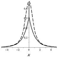
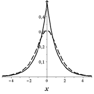
Fig.1 shows the comparative behavior of the fundamental solution for $n=1$ for the cases $\sigma=0$ and $\sigma>0$ at different times.

Figure 1. Fundamental solution for $k=1$, $\beta=1$, $n=1$ for $\sigma=0$ (solid) and $\sigma>0$ (dash). Left: $t=0.5$, right: $t=100$.

Figure 2. Dynamics of density with initial data (23) (left) and (24) (right) at $a=2$, $k=1$, $\beta=1$, $\sigma=0$, $n=1$ at times $t=0$ (dash-dot), $t=1$ (dash), $t=10$ (solid).

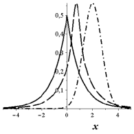
3. Given some initial data, we can compute the convolution (3) and obtain an explicit expression for the density $P(t,x)$. For example, this can be done with the initial Gaussian density distribution

$$P|_{t=0}=\frac{1}{\sqrt{\pi}}e^{-(x-a)^{2}}.$$ (23)

For example, for $\sigma=0$

$${P}(t,x)=\frac{k(1-e^{-2\beta t})}{4}e^{\frac{k^{2}e^{-2\beta t}}{4}}({\rm Erf}X-1)e^{-k|x-e^{-\beta t}a|}+\frac{e^{-\beta t}}{\sqrt{\pi}}e^{-(x-ae^{-\beta t})^{2}},$$

$$X=-xe^{\beta t}+\frac{1}{2}ke^{-\beta t}+a.$$

It is easy to see that the limit of density as $t\to\infty$ coincides with (22), and a weak discontinuity of the initially infinitely smooth solution exists for all $t>0$. Fig.2, left, shows the evolution of the Gaussian density over time.

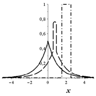
4. It is quite interesting to trace the evolution of a discontinuous density. Let us choose as initial data a piecewise constant function

$$P|_{t=0}=\Theta\left(x+a+\frac{1}{2}\right)-\Theta\left(x+a-\frac{1}{2}\right),\quad a=\rm const,$$ (24)

where $\Theta$ is the Heaviside function. The convolution (3) can be also obtained explicitly. For $\sigma=0$ it is

$$P(t,x)=C_{0}(t)+C_{1}(t)\Theta(\xi_{+})+C_{2}(t)\Theta(\xi_{-})+C_{3}(t)\Theta(\eta_{+})+C_{4}(t)\Theta(\eta_{-}),$$

$$\xi_{\pm}=x+\left(a\pm\frac{1}{2}\right)e^{-\beta t},\quad\eta_{\pm}=x+\frac{1}{2}e^{-\beta t},$$

we do not write down the time-dependent coefficients $C_{i}$, $i=0,\dots,4.$ Fig.2, right, shows the evolution of the step density over time. Note that the jumps are preserved for all $t>0$, but their amplitude tends to zero for $t\to\infty$.

Remark 2.

In the case of $\sigma>0$ the density belongs to $C^{\infty}$ for every $t>0$ for all integrable data, even discontinuous ones, this follows from the fact that the fundamental solution belongs to $C^{\infty}$.

5. Discussion

Note that there are other models that describe non-standard diffusion, in particular, in terms of fractional derivatives (see [17], [18] for an exhaustive review and a detailed list of applications for which there is experimental evidence for the insufficiency of the usual Wiener process). For such models, in some cases it is also possible to construct exact stationary density distributions, as a rule, expressed in special functions [17]. In particular, for the case of subdiffusion (slower than Gaussian), phenomena similar to the presence of pure jumps also arise. This is, in particular, the non-smoothness of the density function.

The method we use can be generalized to the multidimensional case, including for asymmetric diffusion. The method can also be modified for the case of anomalous diffusion by replacing the $\Delta$ operator with $-\sqrt{-\Delta}$ in the equation for the probability density (2). However, the fundamental solution in this case is not as simple as above, it can be expressed in terms of exponential integrals.

6. Author contributions

Conceptualization, methodology, writing, visualization, supervision, O.R.; investigation and validation, O.R. and N.K.

7. Acknowledgments

O.Rozanova was supported by the Russian Science Foundation under grant no. 23-11-00056, performed at Рeoples’ Friendship University of Russia (RUDN University). N.Krutov was supported by the Moscow Center for Fundamental and Applied Mathematics.

References

• [1] L. Billings, M.I. Dykman, I.B. Schwartz, Thermally activated switching in the presence of non-Gaussian noise, Phys. Rev. E 78, 051122, 2008.
• [2] X. Chen, Y.-M. Kang, Y.-X. Fu, Switches in a genetic regulatory system under multiplicative non-Gaussian noise, Journal of Theoretical Biology, 435, 134-144, 2017.
• [3] R. Cont, P. Tankov, Financial Modeling with Jump Processes. Chapman and Hall, Boca Raton, 2004.
• [4] S. Denisov, W.Horsthemke, P. HΓ€nggi, Generalized Fokker-Planck equation: Derivation and exact solutions, Eur. Phys. J. B 68, 567–575, 2009.
• [5] M. Ferreira, N. Vieira, Fundamental solutions of the time fractional diffusion-wave and parabolic Dirac operators. J. Math. Anal. Appl. 2016 (447) 329–353.
• [6] G.-R. Huang, D.B. Saakian, O.S. Rozanova, J.-L. Yu, C.-K. Hu, Exact solution of master equation with Gaussian and compound Poisson noises, J. Stat. Mech. P11033, 2014.
• [7] C. Gardiner, Stochastic Methods: A Handbook for the Natural and Social Sciences. Springer, 2009.
• [8] B. Gaviraghi, M. Annunziato, A. Borzi, Analysis of splitting methods for solving a partial integro-differential Fokker–Planck equation, Applied Mathematics and Computation, 294, 1-17, 2017.
• [9] A. Grigoryan, Y. Kondratiev, A. Piatnitski, E. Zhizhina, Pointwise estimates for heat kernels of convolution-type operators, Proceedings of the London Mathematical Society, 117 (4), 849-880, 2018.
• [10] V. Knopova, A. Kulik, Parametrix construction for certain LΓ©vy-type processes, Random Operators and Stochastic Equations, 23 (2) 111-136, 2015.
• [11] S. Kogan, Electronic Noise and Fluctuations in Solids 2nd edn (Cambirdge: Cambridge University Press), 2008.
• [12] F. KΓΌhn, Transition probabilities of LΓ©vy-type processes: Parametrix construction, Mathematische Nachrichten, 1–19, 2018.
• [13] Y. Luchko, On some new properties of the fundamental solution to the multi-dimensional space- and time-fractional diffusion-wave equation, Mathematics 2017, 5(4), 76.
• [14] F.Mainardi, Y. Luchko, G. Pagnini, The fundamental solution of the space-time fractional diffusion equation. Fract. Calc. Appl. Anal. 2001, 4, 153–192.
• [15] R.A. Maller, G. MΓΌller, A. Szimayer, Ornstein–Uhlenbeck processes and extensions. In: Mikosch, T., Kreiß, JP., Davis, R., Andersen, T. (eds) Handbook of Financial Time Series. Springer, Berlin, Heidelberg, 2009.
• [16] N.F. Marko, R.J. Weil, Non-Gaussian distributions affect identification of expression patterns, functional annotation, and prospective classification in human cancer genomes. PLoS ONE 7(10), e46935, 2012.
• [17] R. Metzler, J. Klafter, The random walk’s guide to anomalous diffusion: a fractional dynamics approach, Physics Reports, 339, 1-77, 2000.
• [18] E. Lemaitre, I.M. Sokolov, R.Metzler, A.V. Chechkin, Non-Gaussian displacement distributions in models of heterogeneous active particle dynamics, New J. Phys. 25, 013010, 2023.
• [19] S. Peszat, LΓ©vy–Ornstein–Uhlenbeck transition semigroup as second quantized operator, Journal of Functional Analysis, 260, 12, (3457-3473), 2011.
• [20] J. Picard, On the existence of smooth densities for jump processes, Probab. Theory Related Fields, 105, 481-511, 1996.
• [21] E. Priola, J. Zabczyk, Densities for Ornstein-Uhlenbeck processes with jumps, Bulletin of the London Mathematical Society 41(1), 2008.
• [22] O.V. Rudenko, A.A. Dubkov, S. N. Gurbatov On exact solutions to the Kolmogorov–Feller equation Doklady Mathematics, 94(1) 476-479, 2016.
• [23] Z. Schuss, Theory and Applications of Stochastic Processes: an Analytical Approach. Springer, 2010.
• [24] G. Wang, Y. Wu, F. Xiao, Z. Ye, Y. Jia, Non-Gaussian noise and autapse-induced inverse stochastic resonance in bistable Izhikevich neural system under electromagnetic induction, Physica A: Statistical Mechanics and its Applications, 598, 127274, 2022.
• [25] A. Yang, H. Wang, T. Zhang, S. Yuan, Stochastic switches of eutrophication and oligotrophication: Modeling extreme weather via non-Gaussian LΓ©vy noise, Chaos, 32, 043116, 2022.