Learning Against Distributional Uncertainty: On the Trade-off Between Robustness and Specificity

Abstract

Trustworthy machine learning aims at combating distributional uncertainties in training data distributions compared to population distributions. Typical treatment frameworks include the Bayesian approach, (min-max) distributionally robust optimization (DRO), and regularization. However, two issues have to be raised: 1) All these methods are biased estimators of the true optimal cost; 2) the prior distribution in the Bayesian method, the radius of the distributional ball in the DRO method, and the regularizer in the regularization method are difficult to specify. This paper studies a new framework that unifies the three approaches and that addresses the two challenges mentioned above. The asymptotic properties (e.g., consistency and asymptotic normalities), non-asymptotic properties (e.g., unbiasedness and generalization error bound), and a Monte–Carlo-based solution method of the proposed model are studied. The new model reveals the trade-off between the robustness to the unseen data and the specificity to the training data.

1 Introduction

Supervised machine learning can be modeled by the following optimization problem (Bousquet and Elisseeff, 2002; Kuhn et al., 2019):

$$\min_{\bm{x}\in\mathcal{X}}~{}\mathbb{E}_{\mathbb{P}_{0}}h(\bm{x},\mathbf{\xi}),$$ (1)

in which $\bm{x}\in\mathcal{X}\subseteq\mathbb{R}^{l}$ is the decision vector and $\mathbf{\xi}\in\Xi\subseteq\mathbb{R}^{m}$ is the random parameter whose underlying distribution is $\mathbb{P}_{0}$; the cost function is denoted by $h:\mathcal{X}\times\Xi\to\mathbb{R}$ (particularly $\mathbb{R}_{+}$). Specifically, hypotheses are parameterized by $\bm{x}$ and $\mathbf{\xi}\coloneqq({\bm{X}},{\bm{Y}})$ denotes a data pair where ${\bm{X}}$ and ${\bm{Y}}$ denote the feature and the expected response, respectively.

In machine learning practice, the true population distribution $\mathbb{P}_{0}$ is unknown, and the empirical distribution $\hat{\mathbb{P}}_{n}:=\frac{1}{n}\sum^{n}_{i=1}\delta_{\mathbf{\xi}_{i}}$, where $\delta_{\mathbf{\xi}_{i}}$ is the Dirac distribution concentrated at the point $\mathbf{\xi}_{i}$, constructed by $n$ independent and identically distributed (i.i.d.) samples $\{\xi_{i}\}_{i\in[n]}$ is the most commonly used estimate of $\mathbb{P}_{0}$. As a result, we can use the data-driven nominal model (Kuhn et al., 2019)

$$\min_{\bm{x}\in\mathcal{X}}\mathbb{E}_{\hat{\mathbb{P}}_{n}}h(\bm{x},\mathbf{\xi})$$ (2)

as an approximation to the true model (1) to find the optimal decision. In the literature, (2) is known as an empirical risk minimization (ERM) model or a sample-average approximation (SAA) model. However, there exists a distributional mismatch (also known as distributional uncertainty) between $\hat{\mathbb{P}}_{n}$ and $\mathbb{P}_{0}$ due to scarce data and the approximation error of (2) to (1) vanishes only when $n\to\infty$. Neglecting such distributional uncertainty in $\hat{\mathbb{P}}_{n}$ may cause significant performance degradation: $\mathbb{E}_{\mathbb{P}_{0}}h(\hat{\bm{x}}_{n},\mathbf{\xi})$ may be significantly larger than $\min_{\bm{x}}\mathbb{E}_{\mathbb{P}_{0}}h(\bm{x},\mathbf{\xi})$ due to overfitting, where $\hat{\bm{x}}_{n}$ solves (2). Mitigating the adverse impact resulting from the distributional uncertainty in $\hat{\mathbb{P}}_{n}$ and controlling the generalization errors, e.g.,

$$\mathbb{E}_{\mathbb{P}^{n}_{0}}\left[\mathbb{E}_{\mathbb{P}_{0}}h(\hat{\bm{x}}_{n},\mathbf{\xi})-\mathbb{E}_{\hat{\mathbb{P}}_{n}}h(\hat{\bm{x}}_{n},\mathbf{\xi})\right],$$ (3)

lie in the core of trustworthy machine learning, where $\mathbb{P}^{n}_{0}$ is the joint distribution of $n$ i.i.d. training samples.

1.1 Literature Review

Suppose $\mathcal{C}$ is a family of admissible distributions on the measurable space $(\Xi,\mathcal{B}_{\Xi})$ where $\mathcal{B}_{\Xi}$ denotes the Borel $\sigma$-algebra on $\Xi$; in the literature, $\mathcal{C}$ is also called an ambiguity set. Considering the nominal problem (2), $\mathcal{C}$ is usually defined as a closed distributional ball with center $\hat{\mathbb{P}}_{n}$ and radius $\epsilon_{n}$, i.e., $\mathcal{C}:=B_{\epsilon_{n}}(\hat{\mathbb{P}}_{n})$. Bayesian approaches attempt to design a probability measure $\mathbb{Q}$ on $(\mathcal{C},\mathcal{B}_{\mathcal{C}})$, where $\mathcal{B}_{\mathcal{C}}$ denotes the Borel $\sigma$-algebra on $\mathcal{C}$ (Gaudard and Hadwin, 1989), and the Bayesian counterpart for the nominal problem (2) is solved:

$$\min_{\bm{x}\in\mathcal{X}}\mathbb{E}_{\mathbb{Q}}\mathbb{E}_{\mathbb{P}}h(\bm{x},\mathbf{\xi}).$$ (4)

Note that the random probability measure $\mathbb{P}$ is distributed according to $\mathbb{Q}$. In this case, the true population distribution $\mathbb{P}_{0}$ is expected to be included in $\mathcal{C}$ and an ideal $\mathbb{Q}$ should be the one that lets the distributions in $\mathcal{C}$ concentrate at $\mathbb{P}_{0}$.

Regularization approaches are another promising choice to hedge against the distributional uncertainty in $\hat{\mathbb{P}}_{n}$ (Vapnik, 1998, Sec. A1.3). To be specific, a regularization term $f(\bm{x})$ is employed and the regularized counterpart

$$\min_{\bm{x}\in\mathcal{X}}\mathbb{E}_{\hat{\mathbb{P}}_{n}}h(\bm{x},\mathbf{\xi})+\lambda f(\bm{x})$$ (5)

for the nominal empirical risk minimization problem (2) is studied, in which $\lambda\geq 0$ is a balancing coefficient. For example, the regularizer $f(\bm{x})$ can be a proper norm $\|\bm{x}\|$ on $\mathcal{X}$ (Goodfellow et al., 2016, Chap. 7), and $\lambda$ may depend on the sample size $n$. Regularization methods are believed to be able to hedge against “overfitting” and reduce generalization errors in a great number of learning problems.

The (min-max) distributionally robust optimization (DRO) counterpart

$$\min_{\bm{x}\in\mathcal{X}}\max_{\mathbb{P}\in\mathcal{C}}\mathbb{E}_{\mathbb{P}}h(\bm{x},\mathbf{\xi})$$ (6)

for the nominal model (2) is another potential approach to handle the distributional uncertainty in $\hat{\mathbb{P}}_{n}$ (Rahimian and Mehrotra, 2022). If the distributional family $\mathcal{C}$ contains the true distribution $\mathbb{P}_{0}$, then the true cost of the decision $\bm{x}$ evaluated at $\mathbb{P}_{0}$, i.e., $\mathbb{E}_{\mathbb{P}_{0}}h(\bm{x},\mathbf{\xi})$, would also be reduced through minimizing the worst-case cost $\max_{\mathbb{P}\in\mathcal{C}}\mathbb{E}_{\mathbb{P}}h(\bm{x},\mathbf{\xi})$ because the inequality $\mathbb{E}_{\mathbb{P}_{0}}h(\bm{x},\mathbf{\xi})\leq\max_{\mathbb{P}\in\mathcal{C}}\mathbb{E}_{\mathbb{P}}h(\bm{x},\mathbf{\xi})$ holds for all $\bm{x}$; for more interpretations and justifications of the DRO method, see Kuhn et al. (2019).

A detailed and more informative version of the literature review is placed in Appendix A.1.

1.2 Research Gaps and Motivations

The DRO approach, SAA approach, and regularized SAA approach are biased estimators of the true optimal objective value (1) when $n$ is finite, i.e. the expected excess risk (the expected value of the difference between the estimated cost and the true optimal cost) are non-zero; the biases only vanish asymptotically (i.e., as $n\to\infty$). Hence, the first motivation of this work is to design a new model that is able to be unbiased for every finite $n$, and hence, the expected excess risk can be controlled to zero.

In addition, it is practically uneasy to specify the prior distribution $\mathbb{Q}$ in the Bayesian method (4), the regularizer $f(\bm{x})$ in the regularization method (5), and the radius $\epsilon_{n}$ of the distributional ball $B_{\epsilon_{n}}(\hat{\mathbb{P}}_{n})$ in the DRO method (6). The three quantities cannot be arbitrarily specified, otherwise, the performances of the three associated methods cannot be guaranteed. For example, $\epsilon_{n}$ can neither be too large nor too small. A small radius cannot guarantee $\mathbb{P}_{0}$ to be included in $\mathcal{C}$, and as a result, the worst-case cost (6) cannot provide an upper bound for the true optimal cost (1). Conversely, if the radius is too large, the DRO methods would become overly conservative and the upper bound of the true optimal cost specified by (6) may be extremely loose. Therefore, the second motivation of this work is to design a new framework that frees us from the elaborate selection of the prior distribution $\mathbb{Q}$, the regularizer $f(\bm{x})$, and the radius $\epsilon_{n}$.

1.3 Contributions

This paper makes the following two contributions.

1. A new framework that can combat the distributional uncertainty in $\hat{\mathbb{P}}_{n}$ is designed; see Section 3 and Model (10). The framework generalizes the Bayesian method (4), the regularization method (5), and the DRO method (6) and suggests the instructions in designing $\mathbb{Q}$, $f(\bm{x})$, and $\epsilon_{n}$; see Remarks 3.1 and 3.6. Moreover, the framework reveals that there exists a trade-off between the robustness to the unseen data (i.e., the adverse distributional uncertainty in $\hat{\mathbb{P}}_{n}$) and the specificity to the training data (i.e., the exploitable empirical information in $\hat{\mathbb{P}}_{n}$); see Remark 3.2. Associated properties of the new model such as consistencies, asymptotic normalities, unbiasedness, and generalization error bounds are derived; see Theorems 3.3, 3.4, and 3.5.

2. A Monte–Carlo-based approach to solve the proposed new model is studied; see Section 4. As a byproduct, we show, by the law of large numbers and linear programming theory, that the proposed solution method is able to reproduce existing results in DRO that are derived from the Monge–Kantorovich duality theory; see Subsection 4.1.1, especially Theorems 4.2 and 4.3.

1.4 Notations And Paper Structure

A full list of notation is placed in Appendix A.2. In Section 2, necessary preliminaries are provided. Section 3 presents the new model and its asymptotic and non-asymptotic properties. In Section 4, the solution method of the new model is studied. The experiments based on the real-world MNIST dataset to validate the power of the proposed new model are conducted in Section 5. Section 6 concludes the paper.

2 Preliminaries

Distributionally robust optimization theory is reviewed in Appendices B.1 and B.2. Statistical concepts including Glivenko–Cantelli class, Donsker class, and Brownian bridge are reviewed in Appendix B.3. As these materials are standard in statistical machine learning, they are excluded from the main body of the paper. In this section, we focus on the Bayesian model (4): i.e., $\min_{\bm{x}}\mathbb{E}_{\mathbb{Q}}\mathbb{E}_{\mathbb{P}}h(\bm{x},\mathbf{\xi})$.

2.1 Mean Distribution

Suppose that $\mathbb{Q}$ is a distribution on $(\mathcal{C},\mathcal{B}_{\mathcal{C}})$ where $\mathcal{C}\subseteq\mathcal{M}(\Xi)$ and $\mathcal{M}(\Xi)$ contains all distributions on $(\Xi,\mathcal{B}_{\Xi})$. If the mean distribution of $\mathbb{Q}$ is $\bar{\mathbb{P}}$, we have $\bar{\mathbb{P}}(E)=\int_{\mathbb{R}}\mathbb{P}(E)\mathbb{Q}(\mathrm{d}\mathbb{P}(E)),~{}\forall E\in\mathcal{B}_{\Xi}$. In other words, the mean distribution is a mixture of distributions in $\mathcal{C}$ with mixing weights determined by $\mathbb{Q}$. Note that, for an event $E$ in $\mathcal{B}_{\Xi}$, $\mathbb{P}(E)$ is a random variable taking values on $\mathbb{R}_{+}$ and its distribution is determined by $\mathbb{Q}$.

Lemma 2.1 (Thm. 3 of Wang et al. (2022)).

If $\bar{\mathbb{P}}$ is the mean of $\mathbb{Q}$ and $\mathbb{E}_{\mathbb{Q}}\mathbb{E}_{\mathbb{P}}|h(\bm{x},\mathbf{\xi})|<\infty$, we have $\mathbb{E}_{\mathbb{Q}}\mathbb{E}_{\mathbb{P}}h(\bm{x},\mathbf{\xi})=\mathbb{E}_{\bar{\mathbb{P}}}h(\bm{x},\mathbf{\xi})$, for every $\bm{x}$. $\square$

2.2 Dirichlet-Process Prior

The most popular choice for the non-parametric prior distribution $\mathbb{Q}$ of $\mathbb{P}$, in Bayesian nonparametrics, is the Dirichlet-process prior. Upon collecting $n$ i.i.d. samples form $\mathbb{P}_{0}$, the posterior non-parametric distribution of $\mathbb{P}$ is still a Dirichlet process whose mean distribution is $\frac{\alpha}{\alpha+n}\hat{\mathbb{P}}+\frac{n}{\alpha+n}\hat{\mathbb{P}}_{n},$ where $\hat{\mathbb{P}}$ is an a priori guess of $\mathbb{P}_{0}$ and $\alpha\geq 0$ is employed to quantify our trust level towards $\hat{\mathbb{P}}$ (Ferguson, 1973), (Ghosal and Van der Vaart, 2017, Chap. 3). To clarify further, if we trust the prior $\hat{\mathbb{P}}$ more than the empirical distribution $\hat{\mathbb{P}}_{n}$, the value of $\alpha$ should be large. For more information on the Dirichlet-process prior, refer to, e.g., Wang et al. (2022, Sec. 3.2). When the Dirichlet-process prior is utilized, as a result of Lemma 2.1, the Bayesian model (4) becomes

$$\min_{\bm{x}}\frac{\alpha}{\alpha+n}\mathbb{E}_{\hat{\mathbb{P}}}h(\bm{x},\mathbf{\xi})+\frac{n}{\alpha+n}\mathbb{E}_{\hat{\mathbb{P}}_{n}}h(\bm{x},\mathbf{\xi}).$$ (7)

Wang et al. (2022) proposes to generalize (7) into

$$\min_{\bm{x}}\beta_{n}\mathbb{E}_{\hat{\mathbb{P}}}h(\bm{x},\mathbf{\xi})+(1-\beta_{n})\mathbb{E}_{\hat{\mathbb{P}}_{n}}h(\bm{x},\mathbf{\xi}),$$ (8)

where the weight coefficient $\beta_{n}\in[0,1]$ can be different from $\frac{\alpha}{\alpha+n}$, but it requires that $\beta_{n}\to 0$ as $n\to\infty$.

3 New Model

3.1 Motivations And Derivations

For real-world applications, the (non-parametric Bayesian) prior $\mathbb{Q}$ is hard to be specified in a Bayesian model $\min_{\bm{x}}\mathbb{E}_{\mathbb{Q}}\mathbb{E}_{\mathbb{P}}h(\bm{x},\mathbf{\xi})$. This motivates the second-order min-max (or worst-case) Bayesian distributionally robust (BDR) optimization counterpart for the nominal model (2):

$$\min_{\bm{x}}\max_{\mathbb{Q}}\mathbb{E}_{\mathbb{Q}}\mathbb{E}_{\mathbb{P}}h(\bm{x},\mathbf{\xi}),$$ (9)

which is a straightforwardly robustified version of the Bayesian model (4). Model (9) is a combination of a Frequentist method and a Bayesian method: The random measure $\mathbb{P}$ follows the second-order probability measure $\mathbb{Q}$, and therefore, in terms of $\mathbb{P}$, (9) is a Bayesian method; the admissible values of $\mathbb{Q}$ are only assumed to lie in an ambiguity set (which is not explicitly specified here), and therefore, in terms of $\mathbb{Q}$, (9) is a Frequentist method.

The model (8) is of interest in its own right. However, the difficulty in practice is to elegantly design the prior belief $\hat{\mathbb{P}}$. Usually we do not have any prior knowledge to specify $\hat{\mathbb{P}}$, and therefore, the uniform distribution on (a subset of) $\Xi$ can be a possible choice. However, this simple strategy might not be sufficiently convincing. Motivated by the second-order min-max Bayesian distributionally robust optimization counterpart (9) for the nominal model (2), we shall study the worst-case version of (8):

$$\min_{\bm{x}\in\mathcal{X}}\beta_{n}\max_{\mathbb{P}\in B_{\epsilon}(\hat{\mathbb{P}})}\mathbb{E}_{\mathbb{P}}h(\bm{x},\mathbf{\xi})+(1-\beta_{n})\mathbb{E}_{\hat{\mathbb{P}}_{n}}h(\bm{x},\mathbf{\xi}).$$ (10)

Note that the uncertainty in $\mathbb{Q}$ is reflected by the uncertainty in the prior estimate $\hat{\mathbb{P}}$ as $\hat{\mathbb{P}}_{n}$ is determined given $\{\mathbf{\xi}_{i}\}_{i\in[n]}$.

Remark 3.1 (Interpretation of Model (10)).

Model (10) is a Bayesian non-parametric model in terms of the data distribution $\mathbb{P}$ and also a Frequentist distributionally robust optimization model in terms of the distribution $\mathbb{Q}$ of the data distribution; cf. (9). Since (10) is equivalent to $\min_{\bm{x}\in\mathcal{X}}\mathbb{E}_{\hat{\mathbb{P}}_{n}}h(\bm{x},\mathbf{\xi})+\frac{\beta_{n}}{1-\beta_{n}}\max_{\mathbb{P}\in B_{\epsilon}(\hat{\mathbb{P}})}\mathbb{E}_{\mathbb{P}}h(\bm{x},\mathbf{\xi}),$ by letting $\lambda_{n}:=\frac{\beta_{n}}{1-\beta_{n}}$ and $f(\bm{x}):=\max_{\mathbb{P}\in B_{\epsilon}(\hat{\mathbb{P}})}\mathbb{E}_{\mathbb{P}}h(\bm{x},\mathbf{\xi})$, (10) can be rewritten as $\min_{\bm{x}\in\mathcal{X}}\mathbb{E}_{\hat{\mathbb{P}}_{n}}h(\bm{x},\mathbf{\xi})+\lambda_{n}f(\bm{x}),$ which is a regularized SAA model (5). Also, when $\beta_{n}:=1$, (10) reduces to a DRO model (6); when $\beta_{n}:=0$, (10) reduces to a SAA model (2). Hence, the new model (10) is a generalized model that unifies the SAA (2), the Bayesian method (4), the regularized SAA (5), and the DRO model (6). The benefit is that (10) suggests how to design $\mathbb{Q}$ in the Bayesian method (4) and $f(\bm{x})$ in the regularization method (5). $\square$

3.2 Data-Driven Case

In practice, it is uneasy to specify $\hat{\mathbb{P}}$. Alternatively, if the distributional ambiguity set is constructed around $\hat{\mathbb{P}}_{n}$ rather than $\hat{\mathbb{P}}$, the model (10) becomes completely data-driven:

$$\min_{\bm{x}\in\mathcal{X}}\beta_{n}\max_{\mathbb{P}\in B_{\epsilon_{n}}(\hat{\mathbb{P}}_{n})}\mathbb{E}_{\mathbb{P}}h(\bm{x},\mathbf{\xi})+(1-\beta_{n})\mathbb{E}_{\hat{\mathbb{P}}_{n}}h(\bm{x},\mathbf{\xi}).$$ (11)

This is a change-of-center trick for the employed distributional ambiguity set: Non-rigorously speaking, we are assuming $\hat{\mathbb{P}}$ is contained in $B_{\epsilon_{n,1}}(\hat{\mathbb{P}}_{n})$ and $\hat{\mathbb{P}}_{n}$ is contained in $B_{\epsilon_{n,2}}(\hat{\mathbb{P}})$ for some radii $\epsilon_{n,1},\epsilon_{n,2}\geq 0$. We call (11) a Bayesian distributionally robust (BDR) optimization. The new model (11) is likely to be less conservative than the usual DRO model (6), i.e., $\max_{\mathbb{P}\in B_{\epsilon_{n}}(\hat{\mathbb{P}}_{n})}\mathbb{E}_{\mathbb{P}}h(\bm{x},\mathbf{\xi})$.

Remark 3.2 (Robustness-Specificity Trade-off).

Since the objective of (11) balances the worst-case cost specified by DRO and the nominal cost specified by SAA, the new model (11) reveals the trade-off between the robustness to the distributional uncertainty (i.e., unseen data) and the specificity to the empirical information (i.e., training data). $\square$

3.3 Properties of The New Model (11)

This subsection studies the asymptotic and non-asymptotic statistical properties of the new BDR model (11).

3.3.1 Notations

Let the true objective be $v(\bm{x})\coloneqq\mathbb{E}_{\mathbb{P}_{0}}h(\bm{x},\mathbf{\xi})$ and the true optimal solution set be $\mathcal{X}_{0}\coloneqq\operatorname*{argmin}_{\bm{x}\in\mathcal{X}}v(\bm{x})$. Every $\bm{x}_{0}\in\mathcal{X}_{0}$ is a true optimal solution. Let the SAA objective be $v_{n}(\bm{x})\coloneqq\mathbb{E}_{\hat{\mathbb{P}}_{n}}h(\bm{x},\mathbf{\xi})$ and the optimal SAA solution set be $\hat{\mathcal{X}}_{n}\coloneqq\operatorname*{argmin}_{\bm{x}\in\mathcal{X}}v_{n}(\bm{x})$. Every $\hat{\bm{x}}_{n}\in\hat{\mathcal{X}}_{n}$ is an SAA solution. Let the DRO objective be $v_{r,n}(\bm{x})\coloneqq\max_{\mathbb{P}\in B_{\epsilon_{n}}(\hat{\mathbb{P}}_{n})}\mathbb{E}_{\mathbb{P}}h(\bm{x},\mathbf{\xi})$ and the optimal DRO solution set be $\hat{\mathcal{X}}_{r,n}\coloneqq\operatorname*{argmin}_{\bm{x}\in\mathcal{X}}v_{r,n}(\bm{x})$. Every $\hat{\bm{x}}_{r,n}\in\hat{\mathcal{X}}_{r,n}$ is a DRO solution. Let the BDR objective be $v_{b,n}(\bm{x})\coloneqq\beta_{n}\max_{\mathbb{P}\in B_{\epsilon_{n}}(\hat{\mathbb{P}}_{n})}\mathbb{E}_{\mathbb{P}}h(\bm{x},\mathbf{\xi})+(1-\beta_{n})\mathbb{E}_{\hat{\mathbb{P}}_{n}}h(\bm{x},\mathbf{\xi})$ and the optimal BDR solution set be $\hat{\mathcal{X}}_{b,n}\coloneqq\operatorname*{argmin}_{\bm{x}\in\mathcal{X}}v_{b,n}(\bm{x})$. Every $\hat{\bm{x}}_{b,n}\in\hat{\mathcal{X}}_{b,n}$ is a BDR solution. Note that for every $\bm{x}$, $v_{n}(\bm{x})$, $v_{r,n}(\bm{x})$, and $v_{b,n}(\bm{x})$ are random variables because $\hat{\mathbb{P}}_{n}$ is a random measure; $\mathbb{E}_{\mathbb{P}_{0}^{n}}\hat{\mathbb{P}}_{n}=\mathbb{P}_{0}$.

3.3.2 Asymptotic Properties of (11)

We consider the parametric function class

$$\mathcal{H}\coloneqq\{h(\bm{x},\cdot):\Xi\to\mathbb{R}|\bm{x}\in\mathcal{X}\}$$ (12)

indexed by $\mathcal{X}$. The asymptotic properties of the Bayesian distributionally robust model (11) can be given as follows.

Theorem 3.3 (Asymptotic Properties of (11)).

Consider the nominal problem (2) and its Bayesian distributionally robust counterpart (11), If the following conditions hold

1. The DRO objective $v_{r,n}(\bm{x})$ is bounded in $\mathbb{P}^{n}_{0}$-probability and attainable for $\bm{x}\in\mathcal{X}^{\prime}\subseteq\mathcal{X}$;

2. The weight coefficient $\beta_{n}\in[0,1]$ for every $n$ and $\sqrt{n}\beta_{n}\to 0$ as $n\to\infty$;

3. The function class $\mathcal{H}$ in (12) is $\mathbb{P}_{0}$-Glivenko–Cantelli;

4. At least one of the following properties holds for the function $v(\bm{x})=\mathbb{E}_{\mathbb{P}_{0}}h(\bm{x},\mathbf{\xi})$:

   1. $v(\bm{x})$ is continuous on $\mathcal{X}^{\prime}$;

   2. $v(\bm{x})$ has the unique global minimizer $\bm{x}_{0}$ on $\mathcal{X}^{\prime}$;

5. The function class $\mathcal{H}$ in (12) is $\mathbb{P}_{0}$-Donsker;

6. $\mathbb{E}_{\mathbb{P}_{0}}[h(\hat{\bm{x}}_{n},\mathbf{\xi})-h(\bm{x}_{0},\mathbf{\xi})]^{2}\overset{p}{\longrightarrow}0$ as $\hat{\bm{x}}_{n}\overset{p}{\longrightarrow}\bm{x}_{0}$,

then the following statements are true.

1. Point-Wise Consistency of Objective Function. For every $\bm{x}\in\mathcal{X}^{\prime}$, we have $v_{b,n}(\bm{x})\overset{p}{\longrightarrow}v(\bm{x})$ as $n\to\infty$.

2. Consistency of Optimal Value. For every $\hat{\bm{x}}_{b,n}\in\hat{\mathcal{X}}_{b,n}\subseteq\mathcal{X}^{\prime}$ and every $\bm{x}_{0}\in\mathcal{X}_{0}\subseteq\mathcal{X}^{\prime}$, we have $v_{b,n}(\hat{\bm{x}}_{b,n})\overset{p}{\longrightarrow}v(\bm{x}_{0})$ as $n\to\infty$. In other words, $\min_{\bm{x}}v_{b,n}(\bm{x})\overset{p}{\longrightarrow}\min_{\bm{x}}v(\bm{x})$ as $n\to\infty$.

3. Consistency of Optimal Solution. The limit point of any solution sequence $\{\hat{\bm{x}}_{b,n}\}$ of (11) is a solution of the true problem (1) in $\mathbb{P}^{n}_{0}$-probability: $\mathbb{P}_{0}^{n}\{\hat{\mathcal{X}}_{b,n}\subseteq\mathcal{X}_{0}\}\to 1$ as $n\to\infty$.

4. Point-Wise Asymptotic Normality of Objective Function. For every $\bm{x}\subseteq\mathcal{X}^{\prime}$, we have $\sqrt{n}[v_{b,n}(\bm{x})-v(\bm{x})]\overset{d}{\longrightarrow}N(0,V_{v,\bm{x}})$ as $n\to\infty$, where $V_{v,\bm{x}}\coloneqq\mathbb{D}_{\mathbb{P}_{0}}h(\bm{x},\mathbf{\xi}),$ the variance of $h(\bm{x},\mathbf{\xi})$ under $\mathbb{P}_{0}$.

5. Asymptotic Normality of Optimal Value. For every $\hat{\bm{x}}_{b,n}\in\hat{\mathcal{X}}_{b,n}\subseteq\mathcal{X}^{\prime}$ and every $\bm{x}_{0}\in\mathcal{X}_{0}\subseteq\mathcal{X}^{\prime}$, if $\hat{\bm{x}}_{b,n}\overset{p}{\longrightarrow}\bm{x}_{0}$, we have $\sqrt{n}[v_{b,n}(\hat{\bm{x}}_{b,n})-v(\bm{x}_{0})]\overset{d}{\longrightarrow}N(0,V_{v})$ as $n\to\infty$, where $V_{v}\coloneqq\mathbb{D}_{\mathbb{P}_{0}}h(\bm{x}_{0},\mathbf{\xi}).$

Proof.

See Appendix C.1. ∎

Note that in conducting minimization over $\bm{x}$, it is sufficient to only consider the subset $\mathcal{X}^{\prime}$ where objective functions are finite-valued. Note also that when the DRO objective $v_{r,n}(\bm{x})$ is finite at $\bm{x}$, the SAA objective $v_{n}(\bm{x})$ and the true objective $v(\bm{x})$ will be finite as well because $\hat{\mathbb{P}}_{n}$ and $\mathbb{P}_{0}$ are included in $B_{\epsilon_{n}}(\hat{\mathbb{P}}_{n})$ for sufficiently large $\epsilon_{n}$. The conditions C1)-C6) in Theorem 3.3 are not restrictive; some practical examples can be seen in Appendix C.2. The asymptotic normality of the optimal solution of the BDR model (11), which requires stronger and therefore more restrictive technical conditions, is deferred to Appendix C.3.

3.3.3 Non-Asymptotic Properties of (11)

The BDR model is unbiased if $\beta_{n}$ can be elegantly given.

Theorem 3.4 (Unbiasedness).

For every $n$, there exists $\beta_{n}\in[0,1]$ such that the BDR-estimated cost $v_{b,n}(\hat{\bm{x}}_{b,n})$ is an unbiased estimate of the true optimal cost $v(\bm{x}_{0})$.

Proof.

We first show that the DRO model is an upward (positively) biased model and the SAA model is a downward (negatively) biased model. Then, the BDR model is proved to be unbiased. For details, see Appendix C.4. ∎

Theorem 3.4 asserts the existence of a $\beta_{n}$ such that the BDR model is unbiased for every $n$. However, the theorem does not inform us of how to find it. In fact, this $\beta_{n}$ is not easy to be found because the biases of the DRO model and the SAA model cannot be easily specified; we only know that the DRO model is positively (i.e., upward) biased and the SAA model is negatively (i.e., downward) biased. Hence, in practice, $\beta_{n}$ is a tuning parameter for every $n$. Possible candidate tuning methods include Bootstrap, etc.

In machine learning, the most important non-asymptotic property of a learning model is the one-sided generalization error bound, that is, the upper bound of the difference between the true cost and the estimated cost. Suppose for every solution $\bm{x}$, with $\mathbb{P}^{n}_{0}$-probability at least $1-\eta$, the true cost $v(\bm{x})$ is upper bounded by the empirical cost as

$$v(\bm{x})\leq\mathcal{G}[v_{n}(\bm{x}),\bm{x},\eta],$$ (13)

where the function $\mathcal{G}$, which takes $v_{n}(\bm{x})$, $\bm{x}$, and $\eta$ as arguments, can be specified by any existing generalization error results such as Hoeffding’s and Bernstein inequalities (Wainwright, 2019, Chaps. 2-3), PAC-Bayesian bounds (Germain et al., 2016, Sec. 2), VC dimensions and Rademacher complexities (Wainwright, 2019, Chap. 4), information-theoretic bounds (Xu and Raginsky, 2017; Wang et al., 2019; Rodríguez Gálvez et al., 2021), among many others (Zhang and Chen, 2021; Wainwright, 2019; Gao, 2022). A concrete example of (13) is given in Appendix C.5.

Theorem 3.5 (Generalization Errors of (11)).

Consider the notations in Subsection 3.3.1 and the empirical error bound (13). The true cost $v(\bm{x})$ of the BDR model is upper bounded, with $\mathbb{P}^{n}_{0}$-probability at least $1-\eta$, as

$$v(\bm{x})\leq\beta_{n}v_{r,n}(\bm{x})+(1-\beta_{n})\mathcal{G}[v_{n}(\bm{x}),\bm{x},\eta],~{}~{}~{}\forall\bm{x}.$$

In particular, focusing on the Bayesian distributionally robust solution $\hat{\bm{x}}_{b,n}$, the true cost $v(\hat{\bm{x}}_{b,n})$ of the BDR model is upper bounded, with $\mathbb{P}^{n}_{0}$-probability at least $1-\eta$, as

$$v(\hat{\bm{x}}_{b,n})\leq\beta_{n}v_{r,n}(\hat{\bm{x}}_{b,n})+(1-\beta_{n})\mathcal{G}[v_{n}(\hat{\bm{x}}_{b,n}),\hat{\bm{x}}_{b,n},\eta].$$

Proof.

Since both the DRO cost $v_{r,n}(\bm{x})$ and the empirical SAA cost $\mathcal{G}[v_{n}(\bm{x}),\bm{x},\eta]$ in (13) give upper bounds for the true cost $v(\bm{x})$, any convex combination of $v_{r,n}(\bm{x})$ and $\mathcal{G}[v_{n}(\bm{x}),\bm{x},\eta]$ is also an upper bound of the true cost $v(\bm{x})$. For detailed proof, see Appendix C.6. ∎

In Theorem 3.5, the latter case is practically more important because it specifies the generalization error of a well-trained model that is adapted to the collected training data.

Remark 3.6 (Easier to Design $\epsilon_{n}$ in BDR Than in DRO).

Theorem 3.5 suggests that the generalization error bound specified by BDR is in-between those specified by DRO and SAA. Hence, when $\epsilon_{n}$ is overly large, i.e., the DRO estimator $v_{r,n}(\bm{x})$ is an extremely conservative estimator of the true cost $v(\bm{x})$, the BDR model can moderate such conservativeness. The motivation is that there exists a type of empirical SAA cost $\mathcal{G}[v_{n}(\bm{x}),\bm{x},\eta]$ such that $\mathcal{G}[v_{n}(\bm{x}),\bm{x},\eta]\leq v_{r,n}(\bm{x})$. A concrete example is given in Appendix C.7. $\square$

On the other hand, since $v(\bm{x})-v_{b,n}(\bm{x})=\beta_{n}[v(\bm{x})-v_{r,n}(\bm{x})]+(1-\beta_{n})[v(\bm{x})-v_{n}(\bm{x})]\leq(1-\beta_{n})[v(\bm{x})-v_{n}(\bm{x})],$ the BDR model gives $1-\beta_{n}$ times smaller estimation bias than the traditional ERM model, for every $\bm{x}$. This justifies the BDR model over the DRO model and the SAA model. Another justification comes with the fact that the DRO model and the SAA model are the special cases of the BDR model, and therefore, if $\beta_{n}$ can be elegantly selected (i.e., well tuned), the performance of the BDR model cannot be worse than those of the DRO model and the SAA model.

3.4 Sectional Summary

The main points in this section are as follows: First, the new BDR model is able to be unbiased (see Theorem 3.4), and therefore, the expected excess risk of the new BDR model is zero; second, the design methods for $\mathbb{Q}$ in (4) and $f(\bm{x})$ in (5) are suggested and justified (see Remarks 3.1), and the radius $\epsilon_{n}$ of the distributional ball is shown to be less important in BDR than in DRO (see Remark 3.6). Therefore, the two challenges raised in Introduction (i.e., Subsection 1.2) have been addressed. Other minor points are as follows: First, the new BDR model generalizes the Bayesian model (4), the regularization model (5), and the DRO model (6) (see Remark 3.1); second, the new BDR model reveals the trade-off between robustness and specificity in statistical learning (see Remark 3.2); third, the new BDR model is asymptotically consistent and normal (see Theorem 3.3).

4 Solution Method

In Subsection 4.1, a novel Monte–Carlo-based solution method is proposed to solve the DRO problem (6). Based on which, we derive the solution method of the new data-driven BDR model (11) in Subsection 4.2.

4.1 Monte–Carlo Approximation

We begin with a generic reference distribution $\bar{\mathbb{P}}$. The special case when $\bar{\mathbb{P}}:=\hat{\mathbb{P}}_{n}$ is discussed in Subsection 4.1.2. In the literature, the DRO problem

$$\begin{array}[]{cc}\displaystyle\min_{\bm{x}\in\mathcal{X}}\max_{\mathbb{P}}&\mathbb{E}_{\mathbb{P}}h(\bm{x},\mathbf{\xi})\\ s.t.&\Delta(\mathbb{P},\bar{\mathbb{P}})\leq\epsilon\end{array}$$ (14)

can be reformulated to a non-linear finite-dimensional reformulation(s). For details, see Appendix B.2.

In this subsection, we propose to use a novel Monte–Carlo-based method to solve (14). Suppose

$$\mathbb{P}\approx\textstyle\sum^{m}_{j=1}\mu_{j}\delta_{\mathbf{\xi}_{j}},$$ (15)

where $\{\mathbf{\xi}_{j}\}_{j\in[m]}$ are samples from $\mathbb{P}$, $\delta_{\mathbf{\xi}_{j}}$ is the Dirac measure at $\mathbf{\xi}_{j}$, and the weights $\{\mu_{j}\}_{j\in[m]}$ can be determined by, e.g., importance sampling through using an appropriate proposal distribution (e.g., uniform distribution) (Bishop and Nasrabadi, 2006, pp. 532). Likewise, we suppose that the set of observations $\{\mathbf{\xi}_{i}\}_{i\in[n]}$ are sampled from $\bar{\mathbb{P}}$ and their weights are $\{\bar{\mu}_{i}\}_{i\in[n]}$ and therefore

$$\bar{\mathbb{P}}\approx\textstyle\sum^{n}_{i=1}\bar{\mu}_{i}\delta_{\mathbf{\xi}_{i}}.$$ (16)

As a result, all integrals in (14), i.e., $\mathbb{E}_{\mathbb{P}}h(\bm{x},\mathbf{\xi})$ and those involved in $\Delta$ if any, can be approximated by weighted sums; the approximations are exact in the weak convergence sense (i.e., sums converge to integrals) if $\min\{n,m\}\to\infty$ due to the law of large numbers. In practice, we may choose large enough values for $n$ and $m$, which however depends on specific problems. As a result, (14) transforms to

$$\begin{array}[]{cl}\displaystyle\min_{\bm{x}}\max_{\{\mu_{j},\mathbf{\xi}_{j}\}_{j\in[m]}}&\sum^{m}_{j=1}\mu_{j}h(\bm{x},\mathbf{\xi}_{j})\\ s.t.&\Delta(\mathbb{P},\bar{\mathbb{P}})\leq\epsilon.\end{array}$$ (17)

If $\Delta$ is the Wasserstein distance, (17) transforms to

$$\begin{array}[]{cl}&\displaystyle\min_{\bm{x}}\max_{\bm{P},\bm{\mu},\{\mathbf{\xi}_{j}\}}\displaystyle\sum^{m}_{j=1}\mu_{j}h(\bm{x},\mathbf{\xi}_{j})\\ s.t.&\sum^{n}_{i=1}\sum^{m}_{j=1}d^{p}(\xi_{i},\xi_{j})\cdot P_{ij}\leq\epsilon^{p}\\ &\sum^{n}_{i=1}P_{ij}=\mu_{j},\quad\quad\forall j\in[m]\\ &\sum^{m}_{j=1}P_{ij}=\bar{\mu}_{i},\quad\quad\forall i\in[n]\\ &P_{ij}\geq 0,\quad\quad\quad\quad\quad\forall i\in[n],\forall j\in[m],\end{array}$$ (18)

where $\bm{P}\coloneqq\{P_{ij}\},\forall i\in[n],\forall j\in[m]$ can be seen as a joint distribution whose marginals are $\bm{\mu}$ and $\bm{\bar{\mu}}$, respectively. The case when $\Delta$ is specified by the $\phi$-divergence is discussed in Appendix D.1. Problem (18) can be reformulated.

Theorem 4.1.

Problem (18) is equivalent to

$$\min_{\bm{x},\lambda_{0}\geq 0}\displaystyle\epsilon^{p}\lambda_{0}+\sum^{n}_{i=1}\bar{\mu}_{i}\max_{\mathbf{\xi}\in\Xi}\left\{h(\bm{x},\mathbf{\xi})-\lambda_{0}d^{p}(\xi,\xi_{i})\right\}.$$ (19)

Proof.

The proof is based on the Lagrange duality theory to equivalently reformulate Problem (18) to Problem (19). For details, see Appendix D.2. ∎

4.1.1 Solve the Inner Maximization of (14)

Theorem 4.2.

Suppose $\mathbb{E}_{\bar{\mathbb{P}}}h(\bm{x},\mathbf{\xi})<\infty$. The inner maximization of (14) under the Wasserstein distance, i.e.,

$$\max_{\mathbb{P}:W_{p}(\mathbb{P},\bar{\mathbb{P}})\leq\epsilon}\int_{\Xi}h(\bm{x},\mathbf{\xi})\mathbb{P}(\mathrm{d}\xi)\\$$ (20)

is equivalent to

$$\min_{\lambda\geq 0}\left\{\lambda\epsilon^{p}+\int_{\Xi}\max_{\mathbf{\xi}\in\Xi}\Big{\{}h(\bm{x},\mathbf{\xi})-\lambda\cdot d^{p}(\mathbf{\xi},\bar{\mathbf{\xi}})\Big{\}}\bar{\mathbb{P}}(\mathrm{d}\bar{\mathbf{\xi}})\right\}.$$ (21)

if and only if the function $h$ has a finite growth rate: For every $\bm{x}$, there exists $0\leq L(\bm{x})<\infty$ such that

$$h(\bm{x},\mathbf{\xi})-h(\bm{x},\mathbf{\xi}_{0})\leq L(\bm{x})d^{p}(\mathbf{\xi},\mathbf{\xi}_{0}),~{}~{}~{}\forall\mathbf{\xi},\mathbf{\xi}_{0}\in\Xi.$$

Proof.

We show that, if $\bm{x}$ is fixed and $\min\{n,m\}\to\infty$, then (18) converges to (20) and (19) converges to (21). Since (18) is equivalent to (19) due to Theorem 4.1 and the equivalence retains asymptotically, we have that (20) is equivalent to (21). For details, see Appendix D.3. ∎

Theorem 4.2 is consistent with the result in Blanchet et al. (2021, Thm. 1) and Gao and Kleywegt (2022, Thm. 1), which is derived using more complicated theories. Note that the condition on the cost function $h$ in Theorem 4.2 is equivalent to the finite-growth-rate condition in Gao and Kleywegt (2022), i.e., (32) in Appendix B.2. If $\bar{\mathbb{P}}$ is discrete, the worst-case distribution solving (20) is given below.

Theorem 4.3.

If $\bar{\mathbb{P}}=\sum^{n}_{i=1}\bar{\mu}_{i}\delta_{\mathbf{\xi}_{i}}$ is supported on $n$ discrete points in $\Xi$, then the worst-case distribution $\mathbb{P}^{*}$ solving (20) is supported on at most $n+1$ points in $\Xi$, that is, there exist $\{\mu_{j},\mathbf{\xi}_{j}\}_{j\in[n+1]}$ such that $\mathbb{P}^{*}=\sum^{n+1}_{j=1}\mu_{j}\delta_{\mathbf{\xi}_{j}}$. Moreover, the discrete worst-case distribution $\mathbb{P}^{*}$ has the following structure

$$\mathbb{P}^{*}=\bar{\mu}_{i_{0}}\cdot[q\delta_{\mathbf{\xi}_{i_{0},1}}+(1-q)\delta_{\mathbf{\xi}_{i_{0},2}}]+\sum^{n}_{j=1,j\neq i_{0}}\bar{\mu}_{j}\delta_{\mathbf{\xi}_{j}},$$ (22)

for one $i_{0}\in[n]$, where $0\leq q\leq 1$ and $\{\mathbf{\xi}_{j}\}_{j\in[n+1]}=\{\mathbf{\xi}_{i_{0,1}}\}\bigcup\{\mathbf{\xi}_{i_{0,2}}\}\bigcup\{\mathbf{\xi}_{i}\}_{i\in[n]-i_{0}}$. To be specific, at most one weight $\bar{\mu}_{i_{0}}$ of $\bar{\mathbb{P}}$ is split into two weights of $\mathbb{P}^{*}$ (N.B.: $q$ is the splitting weight), and the other $n-1$ weights of $\bar{\mathbb{P}}$ (i.e., $\{\bar{\mu}_{i}\}_{i\in[n]-i_{0}}$) are directly inherited by $\mathbb{P}^{*}$.

Proof.

See Appendix D.4. ∎

Theorem 4.3 implies that although $\mathbb{P}^{*}$ and $\bar{\mathbb{P}}$ have slightly different support sets, $\mathbb{P}^{*}$ is almost determined by the discrete reference distribution $\bar{\mathbb{P}}$. Theorem 4.3 is consistent with Yue et al. (2021, Thm. 4), Gao and Kleywegt (2022, Cor. 2), Gao and Kleywegt (2022, Rem. 4), which are derived using rather complicated theories. Instead, the proof of Theorem 4.3 is only based on linear programming theory.

4.1.2 Data-Driven Case

In this section, we exclusively study the data-driven case, that is, $\bar{\mathbb{P}}\coloneqq\hat{\mathbb{P}}_{n}=\frac{1}{n}\sum^{n}_{i=1}\delta_{\mathbf{\xi}_{i}}$ and $\bar{\mu}_{j}=1/n,\forall j\in[n]$.

If $\Delta$ is Wasserstein distance, by eliminating $\bm{\mu}$, (18) gives

$$\begin{array}[]{lll}\displaystyle\min_{\bm{x}}\max_{\bm{P},\{\mathbf{\xi}_{j}\}}&\displaystyle\sum^{m}_{j=1}\sum^{n}_{i=1}h(\bm{x},\mathbf{\xi}_{j})\cdot P_{ij}\\ s.t.&\sum^{m}_{j=1}\sum^{n}_{i=1}d^{p}(\xi_{i},\xi_{j})\cdot P_{ij}\leq\epsilon^{p}\\ &\sum^{m}_{j=1}P_{ij}=\frac{1}{n},\quad\quad\quad\quad\forall i\in[n]\\ &P_{ij}\geq 0,\quad\quad\quad\forall i\in[n],\forall j\in[m].\end{array}$$ (23)

According to Theorem 4.3, when conducting the optimization (23), it is safe to let $m\coloneqq n+1$. Note that the solution method (23) includes several existing duality-based methods as special cases, e.g., Corollary 3.3.1 in Chen et al. (2020), Section 2.2 in Kuhn et al. (2019).

The proposition below recovers a well-known reformulation for (23) in Chen et al. (2020, Cor. 3.3.1), which requires the concavity of $h(\bm{x},\cdot)$, for every $\bm{x}$. However, we can relax the concavity to the continuity.

Theorem 4.4.

Suppose one of the following conditions hold:

1. For every $\bm{x}$, $h(\bm{x},\mathbf{\xi})$ is continuous in $\mathbf{\xi}$ on $\Xi$.

2. For every $\bm{x}$, $h(\bm{x},\mathbf{\xi})$ is concave in $\mathbf{\xi}$ on $\Xi$.

Then, (23) can be reformulated to

$$\begin{array}[]{cll}\displaystyle\min_{\bm{x}}\max_{\{\mathbf{\xi}_{j}\}_{j\in[n]}}&\displaystyle\frac{1}{n}\sum^{n}_{i=1}h(\bm{x},\mathbf{\xi}_{j})\\ s.t.&\frac{1}{n}\sum^{n}_{i=1}d^{p}(\xi_{i},\xi_{j})\leq\epsilon^{p}.\end{array}$$ (24)

Proof.

See Appendix D.5 for the proof based on the intermediate value theorem of a continuous function. Note that in the interior of $\Xi$, concavity implies continuity. ∎

Equipped with the above results, the solution method of the data-driven Bayesian distributionally robust optimization model (11) can be given as follows.

4.2 Solution to the New BDR Model (11)

By letting $m\coloneqq n+1$, the solution of the proposed model (11) is therefore

$$\begin{array}[]{cll}\displaystyle\min_{\bm{x}}\max_{\bm{P},\{\mathbf{\xi}_{j}\}}&\displaystyle\beta_{n}\sum^{n+1}_{j=1}\sum^{n}_{i=1}h(\bm{x},\mathbf{\xi}_{j})\cdot P_{ij}+\\ &\quad\quad(1-\beta_{n})\displaystyle\frac{1}{n}\sum^{n}_{i=1}h(\bm{x},\mathbf{\xi}_{i})\\ s.t.&\sum^{n+1}_{j=1}\sum^{n}_{i=1}d^{p}(\xi_{i},\xi_{j})\cdot P_{ij}\leq\epsilon^{p}\\ &\sum^{n+1}_{j=1}P_{ij}=\frac{1}{n},\quad\quad\quad\quad\forall i\in[n]\\ &P_{ij}\geq 0,\quad\forall i\in[n],\forall j\in[n+1],\end{array}$$ (25)

which is linear over $\bm{P}$. Problem (25) can be solved using the coordinate descent method under proper conditions: fixing $\bm{x}$ and maximizing over $(\bm{P},\{\mathbf{\xi}_{j}\}_{j\in[n+1]})$ and then fixing $(\bm{P},\{\mathbf{\xi}_{j}\}_{j\in[n+1]})$ and minimizing over $\bm{x}$ until converges. Hopefully, with nice conditions, (25) can be transformed into canonical programs such as linear programs; see, e.g., the instance in the experiment in Section 5.

The Lagrange dual form of (25), due to Theorem 4.1, is

$$\begin{array}[]{cll}\displaystyle\min_{\bm{x},\bm{\lambda}}&\displaystyle\beta_{n}\epsilon^{p}\lambda_{0}+\frac{\beta_{n}}{n}\sum^{n}_{i=1}\lambda_{i}+\frac{1-\beta_{n}}{n}\sum^{n}_{i=1}h(\bm{x},\mathbf{\xi}_{i})\\ s.t.&\displaystyle\max_{\mathbf{\xi}\in\Xi}[h(\bm{x},\mathbf{\xi})-\lambda_{0}d^{p}(\xi,\xi_{i})]\leq\lambda_{i},\forall i\in[n],\\ &\lambda_{0}\geq 0,\end{array}$$ (26)

or equivalently, by eliminating $\lambda_{i},i\in[n]$,

$$\begin{array}[]{cll}\displaystyle\min_{\bm{x},\lambda_{0}}&\displaystyle\beta_{n}\epsilon^{p}\lambda_{0}+\frac{\beta_{n}}{n}\sum^{n}_{i=1}\max_{\mathbf{\xi}\in\Xi}\left[h(\bm{x},\mathbf{\xi})-\lambda_{0}d^{p}(\xi,\xi_{i})\right]+\\ &\quad\quad\displaystyle\frac{1-\beta_{n}}{n}\sum^{n}_{i=1}h(\bm{x},\mathbf{\xi}_{i})\\ s.t.&\lambda_{0}\geq 0,\end{array}$$ (27)

which can be solved whenever they are easier than (25).

5 Experiments

We consider three binary classification problems on the MNIST database (LeCun, 1998), aiming at distinguishing three pairs of similar handwritten digits — 1 vs 7, 3 vs 8, and 4 vs 9. In the experiments, we adopt the support vector machine (SVM) as the classification algorithm and solve the problem under the framework of BDR, DRO, and SAA, respectively. The source codes are available online: https://github.com/Haowei-Wang/BDR-Learning.

In this problem, $\mathbf{\xi}$ represents the image-label pair. Each image contains $m=784$ pixels. Denote the $i$-th image pixels vector as ${\bm{I}}_{i}\in\mathbb{R}^{m}$ and its label as $Y_{i}\in\{-1,1\}$, and therefore, $\xi_{i}\coloneqq({\bm{I}}_{i},Y_{i})$. We choose the order-1 Wasserstein distance, i.e. $p=1$, to define a distributional ball; cf. (11); the following metric $d$ is used in the Wasserstein distance (Shafieezadeh-Abadeh et al., 2019, Sec. 3.2):

$$d\left(\mathbf{\xi}_{i},\mathbf{\xi}_{j}\right)=\left\|{\bm{I}}_{i}-{\bm{I}}_{j}\right\|_{\infty}+\kappa\cdot\mathbbm{1}_{\left\{Y_{i}\neq Y_{j}\right\}}$$ (28)

where $\left\|\cdot\right\|_{\infty}$ represents the $\infty$-norm and $\kappa$ quantifies the cost of reversing a label. Hinge loss is used in the SVM, i.e. $h(\bm{x},\xi)\coloneqq\max\{1-Y_{i}\cdot\langle\bm{x},{\bm{I}}_{i}\rangle,~{}0\}$. It can be derived from (26) and Shafieezadeh-Abadeh et al. (2019, Cor. 15) that the BDR formulation is a linear program; see Appendix E.1.

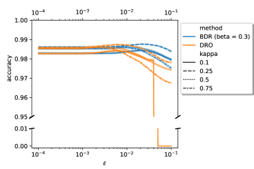
(a) Mean accuracy against $\epsilon$ & $\kappa$

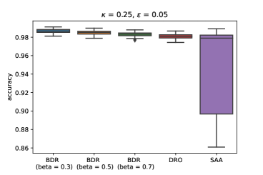
(b) Box plot of accuracy

Figure 1: Average out-of-sample accuracy for 1 vs 7 over 100 independent trials.

We conduct 100 independent trials. For each independent trial, 4/5 of the images are randomly selected to train the model and the remaining 1/5 images are used for testing. The total sample sizes are 15 170, 13 966, and 13 782 for the binary problems of 1 vs 7, 3 vs 8, and 4 vs 9, respectively. For BDR, we choose $\beta$ from $\{0.3,0.5,0.7\}$. For BDR and DRO, the radius $\epsilon$ is chosen from $\{a\times 10^{-b}~{}|~{}a=1,\cdots,9,b=4,3,2\}$ and $\kappa$ is chosen from $\{0.1,0.25,0.5,0.75\}$.

The results of the three problems are very similar. Take the binary problem of 1 vs 7 as an example (the figures for the problems of 3 vs 8 and 4 vs 9 are deferred to Appendix E.2), it can be observed in Figure 1(a) that the performance of BDR and DRO is significantly affected by the values of both $\epsilon$ and $\kappa$. The test accuracy first increases when $\epsilon$ increases but drops afterwards; the peak occurs in the range of $\epsilon\in[0.005,0.05]$. This phenomenon agrees with our claim that the radii of the ambiguity sets can neither be too large nor too small: If the ambiguity sets are too small, robust methods cannot provide sufficient robustness; however, if the ambiguity sets are too large, robust methods are too conservative. Among different values of $\kappa$, we found $\kappa=0.25$ works best for both BDR and DRO. Figure 1(b) shows an accuracy comparison among BDR (with different values of $\beta$), DRO, and SAA, under $\kappa=0.25$ and $\epsilon=0.05$ as explained above. As we can observe, different values of $\beta$ provide very similar good performances, with $\beta=0.3$ having slightly higher accuracy compared to $\beta=0.5$ and $\beta=0.7$. Figure 1(b) also supports our claim that BDR is less conservative than DRO (i.e., designing the radius $\epsilon$ of the involved distributional ball is easier in BDR than in DRO). In addition, the box plots show that SAA has the worst performance with the lowest mean and the highest variance for all three classification problems, while BDR performs consistently the best.

6 Conclusions

In this paper, we propose the BDR (Bayesian Distributionally Robust) framework (10) or (11) that generalizes the Bayesian method, distributionally robust optimization method, and regularization method; see Remark 3.1. The new framework reveals that there exists a trade-off between the robustness to the distributional uncertainty and the specificity to the empirical information; see Remark 3.2. The new framework also suggests the design methods of the prior distribution $\mathbb{Q}$ in the Bayesian method (4) and the regularizer $f(\bm{x})$ in the regularization method (5) (see Remark 3.1), and shows that designing the radius of the involved distributional ball is easier in the new BDR framework than in the existing DRO method (see Remark 3.6 and Figure 1(b)). The asymptotic (i.e., consistencies and asymptotic normalities in Theorem 3.3) and non-asymptotic (i.e., unbiasedness in Theorem 3.4 and generalization error bounds in Theorem 3.5) properties, and the Monte–Carlo-Based solution method of the new framework are studied. Experiments on the real-world dataset MNIST demonstrate that the proposed BDR model outperforms the DRO model and SAA model. Intuitively speaking, the good performance is due to that the BDR model has one more parameter [i.e., the weight $\beta_{n}$ in (10) and (11)] to provide additional flexibility compared to the existing DRO model and the SAA model.

The future research direction is to study alternatives for the Dirichlet-process priors for the second-order probability measure $\mathbb{Q}$ in the Bayesian model (4). This possibly motivates other new robust learning models than the proposed BDR models in (10) and (11). Possible replacements for Dirichlet-process priors are Dirichlet-process mixture priors (Ghosal and Van der Vaart, 2017, Chap. 5), tail-free process priors (Ghosal and Van der Vaart, 2017, Sec. 3.6), among many others.

Appendix A Appendices of Section 1

A.1 Extensive Literature Review

Bayesian methods [Ferguson, 1973, Ghosal and Van der Vaart, 2017] are the first choice to deal with the distributional mismatch in $\hat{\mathbb{P}}_{n}$. As Bayesian statisticians usually do, whenever we have uncertainty in a quantity, we treat this quantity as a random quantity for which a probability distribution is assigned. Suppose $\mathcal{C}$ is a family of admissible distributions on the measurable space $(\Xi,\mathcal{B}_{\Xi})$ where $\mathcal{B}_{\Xi}$ denotes the Borel $\sigma$-algebra on $\Xi$; in the literature, $\mathcal{C}$ is also called an ambiguity set. For instance, in consideration of the nominal problem (2), $\mathcal{C}$ can be defined as a closed distributional ball with center $\hat{\mathbb{P}}_{n}$ and radius $\epsilon_{n}$, that is, $\mathcal{C}:=B_{\epsilon_{n}}(\hat{\mathbb{P}}_{n})$. Bayesian approaches attempt to design a probability measure $\mathbb{Q}$ on $(\mathcal{C},\mathcal{B}_{\mathcal{C}})$, where $\mathcal{B}_{\mathcal{C}}$ denotes the Borel $\sigma$-algebra on $\mathcal{C}$ [Gaudard and Hadwin, 1989], and the following Bayesian counterpart for the nominal problem (2) is solved: $\min_{\bm{x}\in\mathcal{X}}\mathbb{E}_{\mathbb{Q}}\mathbb{E}_{\mathbb{P}}h(\bm{x},\mathbf{\xi})$. Note that the random probability measure $\mathbb{P}$ is distributed according to $\mathbb{Q}$. In this case, the true population distribution $\mathbb{P}_{0}$ is expected to be included in $\mathcal{C}$ and an ideal $\mathbb{Q}$ should be the one that lets the distributions in $\mathcal{C}$ concentrate at $\mathbb{P}_{0}$. Namely, $\mathbb{P}_{0}$ is one of the elements most likely to be sampled from $\mathcal{C}$ according to $\mathbb{Q}$. Under some mild technical conditions, we can find a point $\mathbb{P}^{\prime}\in\mathcal{C}$ satisfying $\mathbb{E}_{\mathbb{Q}}\mathbb{E}_{\mathbb{P}}h(\bm{x},\mathbf{\xi})=\mathbb{E}_{\mathbb{P}^{\prime}}h(\bm{x},\mathbf{\xi})$ for all $\bm{x}$ (see Lemma 2.1). Hence, essentially, Bayesian methods tell us how to locate the “best” candidate in $\mathcal{C}$. If $\mathbb{P}^{\prime}$ is closer to $\mathbb{P}_{0}$ than $\hat{\mathbb{P}}_{n}$ to $\mathbb{P}_{0}$, the Bayesian method (4) would have a smaller approximation error for (1) than the nominal method (2) would have; examples and justifications can be accessed in, e.g., Wu et al. [2018], Anderson and Nguyen [2020]. Note that, in some cases, either (resp. both) $\mathbb{Q}$ or (resp. and) $\mathbb{P}$ can be parametric distributions.

Regularization approaches are another promising choice to hedge against the distributional uncertainty in $\hat{\mathbb{P}}_{n}$ [Vapnik, 1998, Sec. A1.3]. To be specific, a regularization term $f(\bm{x})$ is employed and the regularized counterpart $\min_{\bm{x}\in\mathcal{X}}\mathbb{E}_{\hat{\mathbb{P}}_{n}}h(\bm{x},\mathbf{\xi})+\lambda f(\bm{x})$ for the nominal empirical risk minimization problem (2) is studied, in which $\lambda\geq 0$ is a balancing coefficient. For example, the regularizer $f(\bm{x})$ can be a proper norm $\|\bm{x}\|$ on $\mathcal{X}$ [Goodfellow et al., 2016, Chap. 7], and $\lambda$ may depend on the sample size $n$. Regularization methods are believed to be able to work against “overfitting” and reduce generalization errors in a great number of learning problems; one may reminisce about the “bias-variance trade-off” in the machine learning literature [Hastie et al., 2009, Sec. 2.9]. The rationale of the regularization methods can also be quantitatively justified from many other perspectives such as the stability properties of the learning algorithms [Bousquet and Elisseeff, 2002, Sec. 5.2] and the PAC-Bayesian learning [Germain et al., 2016, Sec. 2], to name a few.

The (min-max) distributionally robust optimization (DRO) counterpart $\min_{\bm{x}\in\mathcal{X}}\max_{\mathbb{P}\in\mathcal{C}}\mathbb{E}_{\mathbb{P}}h(\bm{x},\mathbf{\xi})$ for the nominal model (2) is another potential approach to handle the distributional uncertainty in $\hat{\mathbb{P}}_{n}$ [Rahimian and Mehrotra, 2022]. If the distributional family $\mathcal{C}$ contains the true distribution $\mathbb{P}_{0}$, then the true cost of the decision $\bm{x}$ evaluated at $\mathbb{P}_{0}$, i.e., $\mathbb{E}_{\mathbb{P}_{0}}h(\bm{x},\mathbf{\xi})$, would also be reduced through minimizing the worst-case cost $\max_{\mathbb{P}\in\mathcal{C}}\mathbb{E}_{\mathbb{P}}h(\bm{x},\mathbf{\xi})$ because the inequality $\mathbb{E}_{\mathbb{P}_{0}}h(\bm{x},\mathbf{\xi})\leq\max_{\mathbb{P}\in\mathcal{C}}\mathbb{E}_{\mathbb{P}}h(\bm{x},\mathbf{\xi})$ holds for all $\bm{x}$; for more interpretations and justifications of the DRO method, see Kuhn et al. [2019]. According to, e.g., Yue et al. [2021], Mohajerin Esfahani and Kuhn [2018], we can find a point $\mathbb{P}^{\prime}$ in $\mathcal{C}$ such that $\max_{\mathbb{P}\in\mathcal{C}}\mathbb{E}_{\mathbb{P}}h(\bm{x},\mathbf{\xi})=\mathbb{E}_{\mathbb{P}^{\prime}}h(\bm{x},\mathbf{\xi})$, for all $\bm{x}\in\mathcal{X}$, if some mild technical conditions on the function $h$ can be satisfied. Therefore, as an alternative to the Bayesian approach (4), the DRO approach (6) chooses the “best” candidate $\mathbb{P}^{\prime}$ in $\mathcal{C}$ from another perspective. However, in the practice of DRO methods, elegantly specifying the size parameter $\epsilon_{n}$ of the employed ambiguity set $B_{\epsilon_{n}}(\hat{\mathbb{P}}_{n})=:\mathcal{C}$ is not easy because the radius can neither be too large nor too small. A small radius cannot guarantee $\mathbb{P}_{0}$ to be included in $\mathcal{C}$. Consequently, the worst-case cost (6) cannot provide an upper bound for the true optimal cost (1). Conversely, if the radius is too large, the DRO methods would become overly conservative and the upper bound of the true optimal cost specified by (6) may be extremely loose. Typical design methods for $\epsilon_{n}$ and their drawbacks are as follows.

1. The measure concentration bounds in, e.g., Fournier and Guillin [2015] and Kuhn et al. [2019], are just theoretical results, far away from practical utilization, because the involved constants are unknown for the true underlying distributions. Also, measure concentration bounds are not tight. Third, measure concentration bounds are dependent on the dimension of $\mathbf{\xi}$, and therefore, they may face the curse of dimensionality [Gao, 2022].

2. Practical methods such as cross-validation [Mohajerin Esfahani and Kuhn, 2018, p. 156] and bootstrap [Mohajerin Esfahani and Kuhn, 2018, p. 158] are reliable if and only if the data size $n$ is sufficiently large. When $n$ is small, they may not work well [Chernick, 2011, Varoquaux, 2018].

3. Statistical inference methods presented in Blanchet et al. [2019, 2021] also require $n$ to be large because the optimality of the presented methods is established in the asymptotic sense (i.e., when $n\to\infty$).

According to, e.g., Kuhn et al. [2019, Thm. 10], Shafieezadeh-Abadeh et al. [2019], under some technical conditions, the DRO approach (6) amounts to a regularized empirical risk minimization approach (5), which, in a sense, advocates why the DRO approach (6) is able to combat overfitting and provide excellent generalization performance.

A.2 Notations

Notations used in this paper are summarized in Table 1.

Table 1: Notation List

Symbol	Interpretation
$\mathcal{M}(\Xi)$	all distributions on $(\Xi,\mathcal{B}_{\Xi})$ where $\mathcal{B}_{\Xi}$ is the Borel $\sigma$-algebra on $\Xi$
$\mathcal{B}_{\mathcal{M}(\Xi)}$	Borel $\sigma$-algebra on $\mathcal{M}(\Xi)$
$\mathbb{P}_{0}$	true population distribution
$\hat{\mathbb{P}}_{n}$	empirical distribution supported on $n$ i.i.d. samples
$\hat{\mathbb{P}}$	a prior estimate of $\mathbb{P}_{0}$ based on prior knowledge
$\bar{\mathbb{P}}$	reference distribution working as a proper estimate of $\mathbb{P}_{0}$, which can be the empirical $\hat{\mathbb{P}}_{n}$ or the prior $\hat{\mathbb{P}}$, among many others
$\mathbb{P}_{0}^{n}$	$n$-fold product measure induced by $\mathbb{P}_{0}$ (i.e., joint distribution of $n$ i.i.d. samples)
$[n]$	$[n]\coloneqq\{1,2,\ldots,n\}$, the running index set
$\Delta(\mathbb{P},\hat{\mathbb{P}}_{n})$	statistical similarity measure between $\mathbb{P}$ and $\hat{\mathbb{P}}_{n}$; $\Delta$ can be any possible divergences or statistical distances
$B_{\epsilon}(\hat{\mathbb{P}}_{n})$	$\coloneqq\{\mathbb{P}\in\mathcal{M}(\Xi)|\Delta(\mathbb{P},\hat{\mathbb{P}}_{n})\leq\epsilon\}$, closed distributional ball with radius $\epsilon$ and center $\hat{\mathbb{P}}_{n}$
$N(\bm{\mu},\bm{\Sigma})$	Gaussian distribution with mean $\bm{\mu}$ and covariance $\bm{\Sigma}$
$\overset{a.s.}{\longrightarrow}$	converges almost surely
$\overset{p}{\longrightarrow}$	converges in probability
$\overset{d}{\longrightarrow}$	converges in distribution
$o_{p}(1)$	if a sequence $a_{n}=o_{p}(1)$, then $a_{n}$ converges to zero in probability
$d(\bm{x},\bm{y})$	distance between two points $\bm{x}$ and $\bm{y}$
$d(\bm{x},\mathcal{X})$	$\coloneqq\inf_{\bm{y}\in\mathcal{X}}\|\bm{x}-\bm{y}\|$, distance between the point $\bm{x}$ and the set $\mathcal{X}$
$d(\mathcal{X},\mathcal{Y})$	$\coloneqq\sup_{\bm{x}\in\mathcal{X}}d(\bm{x},\mathcal{Y})$, distance between the two sets $\mathcal{X}$ and $\mathcal{Y}$
$\mathbb{E}_{\mathbb{P}}[\cdot],\mathbb{D}_{\mathbb{P}}[\cdot]$	the expectation operator and the covariance operator, respectively, with respect to the distribution $\mathbb{P}$
$\nabla_{\bm{x}}h(\bm{x}_{0},\mathbf{\xi})$	the gradient, i.e., Jacobian, of $h(\bm{x},\mathbf{\xi})$ with respect to $\bm{x}$ evaluated at $\bm{x}_{0}$
$\nabla^{2}_{\bm{x}}h(\bm{x}_{0},\mathbf{\xi})$	the second-order gradient, i.e., Hessian, of $h(\bm{x},\mathbf{\xi})$ with respect to $\bm{x}$ evaluated at $\bm{x}_{0}$
$\bm{V}^{-\top}\coloneqq[\bm{V}^{-1}]^{\top}$	the transpose of the inverse of the matrix $\bm{V}$

Appendix B Appendices of Section 2

B.1 Similarity Measures of Distributions and Distributional Balls

B.1.1 $\phi$-Divergence

Suppose $\mathbb{P}$ is absolutely continuous with respect to $\bar{\mathbb{P}}$. Let $\phi:\mathbb{R}_{+}\to\{\mathbb{R}\cup+\infty\}$ denote a convex function that satisfies $\phi(1)=0$ and $0\phi(0/0)=0$. The $\phi$-divergence (i.e., $f$-divergence) of $\mathbb{P}$ from $\bar{\mathbb{P}}$, generated by $\phi$, is defined as

$$F_{\phi}(\mathbb{P}\|\bar{\mathbb{P}})=\int_{\Xi}\phi\left(\frac{\mathrm{d}\mathbb{P}}{\mathrm{d}\bar{\mathbb{P}}}\right)\bar{\mathbb{P}}(\mathrm{d}\mathbf{\xi}),$$ (29)

where ${\mathrm{d}\mathbb{P}}/{\mathrm{d}\bar{\mathbb{P}}}$ is the Radon–Nikodym derivative of $\mathbb{P}$ with respect to $\bar{\mathbb{P}}$. When $\phi(t)\coloneqq t\ln t$ for all $t>0$, the $\phi$-divergence specifies the well-known Kullback–Leibler divergence; cf. Ben-Tal et al. [2013, Table 2].

A $\phi$-divergence distributional ball with radius $\epsilon\geq 0$ and center $\bar{\mathbb{P}}$ is defined as

$$B_{\epsilon,\phi}(\bar{\mathbb{P}})\coloneqq\{\mathbb{P}\in\mathcal{M}(\Xi)|F_{\phi}(\mathbb{P}\|\bar{\mathbb{P}})\leq\epsilon\}.$$

If $\epsilon=0$, the ball $B_{\epsilon,\phi}(\bar{\mathbb{P}})$ reduces to the singleton that contains only $\bar{\mathbb{P}}$. In some literature, the ball is also defined as $B_{\epsilon,\phi}(\bar{\mathbb{P}})\coloneqq\{\mathbb{P}\in\mathcal{M}(\Xi)|F_{\phi}(\bar{\mathbb{P}}\|\mathbb{P})\leq\epsilon\}$ where $\mathbb{P}$ and $\bar{\mathbb{P}}$ are swapped. The two versions are not equivalent because the $\phi$-divergence is not guaranteed to be symmetric in general.

B.1.2 Wasserstein Distance

The order-$p$ Wasserstein distance between the two distributions $\mathbb{P}$ and $\bar{\mathbb{P}}$ is defined as

$$W_{p}(\mathbb{P},\bar{\mathbb{P}})={\left[\inf_{\pi\in\mathcal{M}(\Xi\times\Xi)}\mathbb{E}_{\pi}d^{p}(\mathbf{\xi}_{1},\mathbf{\xi}_{2})\right]}^{\frac{1}{p}}={\left[\inf_{\pi\in\mathcal{M}(\Xi\times\Xi)}\int_{\Xi\times\Xi}d^{p}(\mathbf{\xi}_{1},\mathbf{\xi}_{2})\pi(\mathrm{d}\mathbf{\xi}_{1},\mathrm{d}\mathbf{\xi}_{2})\right]}^{\frac{1}{p}},$$ (30)

where $d$ is a distance on $\Xi$, $p\geq 1$, and $\pi$ is a joint distribution on $\Xi\times\Xi$ with marginals $\mathbb{P}$ and $\bar{\mathbb{P}}$.

An order-$p$ Wasserstein distributional ball with radius $\epsilon$ and center $\bar{\mathbb{P}}$ is defined as

$$B_{\epsilon,p}(\bar{\mathbb{P}})\coloneqq\{\mathbb{P}\in\mathcal{M}(\Xi)|W_{p}(\mathbb{P},\bar{\mathbb{P}})\leq\epsilon\}.$$

If $\epsilon=0$, the ball $B_{\epsilon,p}(\bar{\mathbb{P}})$ reduces to the singleton that contains only $\bar{\mathbb{P}}$.

Wasserstein balls admit the following concentration properties. Suppose the true population distribution $\mathbb{P}_{0}$ has a light tail: That is, there exist $\alpha>p\geq 1$ (but $p\neq m/2$) and finite $A>0$ such that $\mathbb{E}_{\mathbb{P}_{0}}\left[\exp\left(\|\mathbf{\xi}\|^{\alpha}\right)\right]\leq A$ (recall that $m$ is the length of $\mathbf{\xi}$). Then, there exist constants $c_{1},c_{2}>0$ such that

$$\mathbb{P}_{0}^{n}\left[\mathbb{P}_{0}\in{B}_{\epsilon_{n},p}(\hat{\mathbb{P}}_{n})\right]\geq 1-\eta$$ (31)

holds, for any $\eta\in(0,1]$, when

$$\epsilon_{n}\geq\begin{cases}\left(\frac{\log\left(c_{1}/\eta\right)}{c_{2}n}\right)^{\min\{p/m,1/2\}}&\text{ if }n\geq\frac{\log\left(c_{1}/\eta\right)}{c_{2}},\\ \left(\frac{\log\left(c_{1}/\eta\right)}{c_{2}n}\right)^{p/\alpha}&\text{ if }n<\frac{\log\left(c_{1}/\eta\right)}{c_{2}}.\end{cases}$$

Note that $c_{1}$ and $c_{2}$ are determined by $\alpha$, $A$, and $m$. This result is attributed to Kuhn et al. [2019, Thm. 18]. The difficulty of applying this result in practice is that the involved constants $\alpha$ and $A$ cannot be exactly obtained because the population distribution $\mathbb{P}_{0}$ is unknown, and so are $c_{1}$ and $c_{2}$.

B.2 Wasserstein DRO Models

B.2.1 Existence of The Solution of Wasserstein DRO Models

Suppose $(\Xi,d)$ is a proper, complete, and separable metric space, $h(\bm{x},\mathbf{\xi})$ is upper semi-continuous in $\mathbf{\xi}$ on $\Xi$ and $\mathbb{E}_{\bar{\mathbb{P}}}|h(\bm{x},\mathbf{\xi})|<\infty$ for every $\bm{x}$, and $\bar{\mathbb{P}}$ has a finite $p$-th moment: That is, for every $\mathbf{\xi}_{0}\in\Xi$, we have

$$\int_{\Xi}d^{p}(\mathbf{\xi},\mathbf{\xi}_{0})\bar{\mathbb{P}}(\mathrm{d}\mathbf{\xi})<\infty.$$

Then, for every $\bm{x}$, the optimal value of the Wasserstein DRO problem (20):

$$\max_{\mathbb{P}:W_{p}(\mathbb{P},\bar{\mathbb{P}})\leq\epsilon}\int_{\Xi}h(\bm{x},\mathbf{\xi})\mathbb{P}(\mathrm{d}\xi)\\$$

is finite if and only if there exist $\mathbf{\xi}_{0}\in\Xi$ and $c_{1}(\bm{x})>0$ such that

$$h(\bm{x},\mathbf{\xi})\leq c_{1}(\bm{x})[1+d^{p}(\mathbf{\xi},\mathbf{\xi}_{0})],~{}~{}~{}\forall\mathbf{\xi}\in\Xi.$$ (32)

In addition, the optimal value is attainable (by one $\mathbb{P}^{*}$ such that $W_{p}(\mathbb{P}^{*},\bar{\mathbb{P}})\leq\epsilon$) if there exist $\mathbf{\xi}_{0}\in\Xi$, $c_{1}(\bm{x})>0$, and $c_{2}\in(0,p)$ such that

$$h(\bm{x},\mathbf{\xi})\leq c_{1}(\bm{x})[1+d^{c_{2}}(\mathbf{\xi},\mathbf{\xi}_{0})],~{}~{}~{}\forall\mathbf{\xi}\in\Xi.$$ (33)

The results above are due, e.g., to Yue et al. [2021], Chen et al. [2020]. Note that (32) is in analogy to the Lipschitz continuity which limits the “change rate” of a function. To clarify further, for example, by letting $p\coloneqq 1$ and $d\coloneqq\|\cdot\|$ (i.e., the metric $d$ is induced by a norm $\|\cdot\|$), we can see that (32) is in analogy to $h(\bm{x},\mathbf{\xi})\leq h(\bm{x},\mathbf{\xi}_{0})+L(\bm{x})\|\mathbf{\xi}-\mathbf{\xi}_{0}\|$, for every $\mathbf{\xi},\mathbf{\xi}_{0}\in\Xi$, where $L(\bm{x})>0$ is the Lipschitz constant. For this reason, in literature, e.g., Chen et al. [2020], Gao and Kleywegt [2022], (32) is called the “finite-growth-rate” condition for the function $h$.

In this paper, for practicality, we consistently assume that the condition (33) is satisfied so that it is safe to replace the infimum with the maximum in (20).

B.2.2 Reformulation of Wasserstein DRO Models

According to, e.g., Blanchet et al. [2021, Thm. 1] and Gao and Kleywegt [2022, Thm. 1], the Wasserstein DRO problem (20) is equivalent to its Lagrangian dual (21):

$$\min_{\lambda\geq 0}\left\{\lambda\epsilon^{p}+\int_{\Xi}\max_{\mathbf{\xi}\in\Xi}\Big{\{}h(\bm{x},\mathbf{\xi})-\lambda\cdot d^{p}(\mathbf{\xi},\bar{\mathbf{\xi}})\Big{\}}\bar{\mathbb{P}}(\mathrm{d}\bar{\mathbf{\xi}})\right\}.$$

If $\bar{\mathbb{P}}=\sum^{n}_{i=1}\bar{\mu}_{i}\delta_{\mathbf{\xi}_{i}}$ is a discrete distribution, e.g., an empirical distribution, supported on $n$ points $\{\mathbf{\xi}_{i}\}_{i\in[n]}$, then (21) becomes

$$\min_{\lambda\geq 0}\left\{\lambda\epsilon^{p}+\sum^{n}_{i=1}\bar{\mu}_{i}\max_{\mathbf{\xi}\in\Xi}\Big{\{}h(\bm{x},\mathbf{\xi})-\lambda\cdot d^{p}(\mathbf{\xi},\mathbf{\xi}_{i})\Big{\}}\right\}.$$ (34)

B.2.3 Support Set of Worst-Case Distributions

If $\bar{\mathbb{P}}$ is supported on $n$ points in $\Xi$, then the worst-case distribution solving (20) is supported on at most $n+1$ points in $\Xi$; see Yue et al. [2021, Thm. 4], Gao and Kleywegt [2022, Cor. 2].

B.3 Glivenko–Cantelli Class, Donsker Class, and Brownian Bridge

Consider a function class $\mathcal{F}\coloneqq\{f:\Xi\to\mathbb{R}\}$.

Definition B.1 (Glivenko–Cantelli Class).

Suppose for every $f\in\mathcal{F}$, $\mathbb{E}_{\mathbb{P}_{0}}f(\mathbf{\xi})$ is defined and finite; that is, $f$ is $\mathbb{P}_{0}$-integrable. The function class $\mathcal{F}$ is called $\mathbb{P}_{0}$-Glivenko–Cantelli if

$$\sup_{f\in\mathcal{F}}|\mathbb{E}_{\hat{\mathbb{P}}_{n}}f(\mathbf{\xi})-\mathbb{E}_{\mathbb{P}_{0}}f(\mathbf{\xi})|\overset{a.s.}{\longrightarrow}0.$$ (35)

Intuitively, if $\mathcal{F}$ is a Glivenko–Cantelli class, then the uniform strong law of large numbers holds on $\mathcal{F}$. $\square$

Definition B.2 (Donsker Class).

Consider an empirical process

$$\mathbb{G}_{n}(f)\coloneqq\sqrt{n}[\mathbb{E}_{\hat{\mathbb{P}}_{n}}f(\mathbf{\xi})-\mathbb{E}_{\mathbb{P}_{0}}f(\mathbf{\xi})],~{}~{}~{}\forall f\in\mathcal{F}$$ (36)

indexed by the function class $\mathcal{F}$. That is, $\{\mathbb{G}_{n}(f)|f\in\mathcal{F}\}$ in (36) is a stochastic process indexed by $\mathcal{F}$; the randomness comes from the (random) empirical measure $\hat{\mathbb{P}}_{n}$. Suppose for every $f\in\mathcal{F}$, $\mathbb{D}_{\mathbb{P}_{0}}f(\mathbf{\xi})$ is defined and finite; that is, $f$ is $\mathbb{P}_{0}$-square-integrable. The function class $\mathcal{F}$ is called $\mathbb{P}_{0}$-Donsker if the empirical (stochastic) process $\mathbb{G}_{n}$ converges in distribution to a Brownian bridge (stochastic) process:

$$\mathbb{G}_{n}\overset{d}{\longrightarrow}\mathbb{G}_{\mathbb{P}_{0}},$$ (37)

where $\mathbb{G}_{\mathbb{P}_{0}}$ is a zero-mean $\mathbb{P}_{0}$-Brownian bridge on $\mathcal{F}$ with uniformly continuous sample paths with respect to the semi-metric $\sqrt{\mathbb{D}_{\mathbb{P}_{0}}[f_{1}(\mathbf{\xi})-f_{2}(\mathbf{\xi})]}$ between $f_{1}\in\mathcal{F}$ and $f_{2}\in\mathcal{F}$; in addition, $\mathbb{G}_{\mathbb{P}_{0}}(f)$ is tight for every $f\in\mathcal{F}$; i.e., $\sup_{f\in\mathcal{F}}|\mathbb{G}_{\mathbb{P}_{0}}(f)|<\infty$ in $\mathbb{P}_{0}$-probability. Intuitively, if $\mathcal{F}$ is a Donsker class, then the uniform central limit theorem holds on $\mathcal{F}$. $\square$

A zero-mean $\mathbb{P}_{0}$-Brownian bridge $\mathbb{G}_{\mathbb{P}_{0}}$ on $\mathcal{F}$ is a Gaussian process on $\mathcal{F}$ satisfying the following two conditions:

1. For every $f\in\mathcal{F}$, $\mathbb{G}_{\mathbb{P}_{0}}(f)$ is a random variable with mean of zero and variance of $\mathbb{D}_{\mathbb{P}_{0}}(f)$.

2. For every integer $r$ and every possible collection of functions $\{f_{1},f_{2},\ldots,f_{r}\}$ taken from $\mathcal{F}$, the random vector

   $$[\mathbb{G}_{\mathbb{P}_{0}}(f_{1}),\mathbb{G}_{\mathbb{P}_{0}}(f_{2}),\ldots,\mathbb{G}_{\mathbb{P}_{0}}(f_{r})]^{\top}$$

   follows a $r$-dimensional multivariate Gaussian distribution with covariance between $\mathbb{G}_{\mathbb{P}_{0}}(f_{i})$ and $\mathbb{G}_{\mathbb{P}_{0}}(f_{j})$ being defined as

   $$\mathbb{E}_{\mathbb{P}_{0}}f_{i}\cdot f_{j}-\mathbb{E}_{\mathbb{P}_{0}}f_{i}\cdot\mathbb{E}_{\mathbb{P}_{0}}f_{j},$$

   for every $i,j\in[r]$.

Since the values of the Gaussian process $\mathbb{G}_{\mathbb{P}_{0}}$ at some functions $f\in\mathcal{F}$ are strictly zeros, without any randomness, the Gaussian process $\mathbb{G}_{\mathbb{P}_{0}}$ is called a Brownian bridge because some values are tied, for example, when $f$ is $\mathbb{P}_{0}$-almost everywhere constant.

Appendix C Appendices of Section 3

C.1 Proof of Theorem 3.3

Proof.

For every $\bm{x}\in\mathcal{X}^{\prime}$ such that the SAA and DRO objectives are bounded in $\mathbb{P}^{n}_{0}$-probability, we have

$$v_{b,n}(\bm{x})-v_{n}(\bm{x})=\beta_{n}\max_{\mathbb{P}\in B_{\epsilon_{n}}(\hat{\mathbb{P}}_{n})}\mathbb{E}_{\mathbb{P}}h(\bm{x},\mathbf{\xi})+(1-\beta_{n})\mathbb{E}_{\hat{\mathbb{P}}_{n}}h(\bm{x},\mathbf{\xi})-\mathbb{E}_{\hat{\mathbb{P}}_{n}}h(\bm{x},\mathbf{\xi})\overset{p}{\longrightarrow}0,$$

because $\beta_{n}\to 0$. Hence, by Slutsky’s theorem, $v_{b,n}(\bm{x})$ shares the same asymptotic properties with $v_{n}(\bm{x})$, for every $\bm{x}\in\mathcal{X}^{\prime}$. As a result, Statement S1) and S4) are immediate due to the conventional strong law of large numbers, i.e.,

$$v_{n}(\bm{x})=\mathbb{E}_{\hat{\mathbb{P}}_{n}}h(\bm{x},\mathbf{\xi})\overset{a.s.}{\longrightarrow}\mathbb{E}_{\mathbb{P}_{0}}h(\bm{x},\mathbf{\xi})=v(\bm{x}),~{}~{}~{}\forall x\in\mathcal{X}^{\prime},$$

and the conventional central limit theorem

$$\sqrt{n}[\mathbb{E}_{\hat{\mathbb{P}}_{n}}h(\bm{x},\mathbf{\xi})-\mathbb{E}_{\mathbb{P}_{0}}h(\bm{x},\mathbf{\xi})]\overset{d}{\longrightarrow}N(0,\mathbb{D}_{\mathbb{P}_{0}}h(\bm{x},\mathbf{\xi})),~{}~{}~{}\forall x\in\mathcal{X}^{\prime},$$

respectively.

Suppose the DRO sub-problem is solved by $\bar{\mathbb{P}}_{n}$ such that

$$\mathbb{E}_{\bar{\mathbb{P}}_{n}}h(\bm{x},\mathbf{\xi})=\max_{\mathbb{P}\in B_{\epsilon_{n}}(\hat{\mathbb{P}}_{n})}\mathbb{E}_{\mathbb{P}}h(\bm{x},\mathbf{\xi}),$$

for $\bm{x}\in\mathcal{X}^{\prime}$. Note that this assumption is reasonable due to Condition C1). We have

$$\begin{array}[]{l}\displaystyle\sup_{\bm{x}\in\mathcal{X}^{\prime}}|v_{b,n}(\bm{x})-v(\bm{x})|\\ \quad\quad=\displaystyle\sup_{\bm{x}\in\mathcal{X}^{\prime}}\left|\mathbb{E}_{\beta_{n}\bar{\mathbb{P}}_{n}+(1-\beta_{n})\hat{\mathbb{P}}_{n}}h(\bm{x},\mathbf{\xi})-\mathbb{E}_{\mathbb{P}_{0}}h(\bm{x},\mathbf{\xi})\right|\\ \quad\quad=\displaystyle\sup_{\bm{x}\in\mathcal{X}^{\prime}}\left|\beta_{n}\Big{[}\mathbb{E}_{\bar{\mathbb{P}}_{n}}h(\bm{x},\mathbf{\xi})-\mathbb{E}_{\mathbb{P}_{0}}h(\bm{x},\mathbf{\xi})\Big{]}+(1-\beta_{n})\Big{[}\mathbb{E}_{\hat{\mathbb{P}}_{n}}h(\bm{x},\mathbf{\xi})-\mathbb{E}_{\mathbb{P}_{0}}h(\bm{x},\mathbf{\xi})\Big{]}\right|\\ \quad\quad\leq\displaystyle\beta_{n}\sup_{\bm{x}\in\mathcal{X}^{\prime}}\left|\mathbb{E}_{\bar{\mathbb{P}}_{n}}h(\bm{x},\mathbf{\xi})-\mathbb{E}_{\mathbb{P}_{0}}h(\bm{x},\mathbf{\xi})\right|+(1-\beta_{n})\sup_{\bm{x}\in\mathcal{X}^{\prime}}\left|\mathbb{E}_{\hat{\mathbb{P}}_{n}}h(\bm{x},\mathbf{\xi})-\mathbb{E}_{\mathbb{P}_{0}}h(\bm{x},\mathbf{\xi})\right|\\ \quad\quad\overset{p}{\longrightarrow}0.\end{array}$$

The first term vanishes because $\beta_{n}$ approaches zero and $\sup_{\bm{x}\in\mathcal{X}^{\prime}}\left|\mathbb{E}_{\bar{\mathbb{P}}_{n}}h(\bm{x},\mathbf{\xi})-\mathbb{E}_{\mathbb{P}_{0}}h(\bm{x},\mathbf{\xi})\right|$ is finite on $\mathcal{X}^{\prime}$, whereas the second term decays because $\mathcal{H}$ is $\mathbb{P}_{0}$-Glivenko–Cantelli. As a result, $\min_{\bm{x}}v_{b,n}\overset{p}{\longrightarrow}\min_{\bm{x}}v(\bm{x})$, as $n\to\infty$, because

$$|v_{b,n}(\hat{\bm{x}}_{b,n})-v(\bm{x}_{0})|=\displaystyle|\min_{\bm{x}\in\mathcal{X}^{\prime}}v_{b,n}(\bm{x})-\min_{\bm{x}\in\mathcal{X}^{\prime}}v(\bm{x})|\leq\displaystyle\sup_{\bm{x}\in\mathcal{X}^{\prime}}|v_{b,n}(\bm{x})-v(\bm{x})|\overset{p}{\longrightarrow}0.$$

This is Statement S2).

For every $\hat{\bm{x}}_{b,n}\in\hat{\mathcal{X}}_{b,n}$, we have

$$\begin{array}[]{cl}\displaystyle|v(\hat{\bm{x}}_{b,n})-\min_{\bm{x}\in\mathcal{X}^{\prime}}v(\bm{x})|&\leq\displaystyle|v(\hat{\bm{x}}_{b,n})-v_{b,n}(\hat{\bm{x}}_{b,n})|+\displaystyle|v_{b,n}(\hat{\bm{x}}_{b,n})-\min_{\bm{x}\in\mathcal{X}^{\prime}}v(\bm{x})|\\ &\leq\displaystyle\sup_{\bm{x}\in\mathcal{X}^{\prime}}|v_{b,n}(\bm{x})-v(\bm{x})|+\displaystyle|v_{b,n}(\hat{\bm{x}}_{b,n})-\min_{\bm{x}\in\mathcal{X}^{\prime}}v(\bm{x})|\\ &\overset{p}{\longrightarrow}0.\end{array}$$

Therefore, due to Condition C4), there exists $\bm{x}_{0}\in\mathcal{X}_{0}$ such that $\hat{\bm{x}}_{b,n}\overset{p}{\longrightarrow}\bm{x}_{0}$, which proves Statement S3). (One may use a contradiction, by assuming that the limit point of $\hat{\bm{x}}_{b,n}$ is not in $\mathcal{X}_{0}$, to verify this claim.)

By Conditions C5) and C6), we have $\mathbb{G}_{n}h(\hat{\bm{x}}_{n},\mathbf{\xi})\overset{d}{\longrightarrow}\mathbb{G}_{\mathbb{P}_{0}}h(\bm{x}_{0},\mathbf{\xi})\sim N(0,\mathbb{D}_{\mathbb{P}_{0}}h(\bm{x}_{0},\mathbf{\xi}))$; see Van der Vaart [2000, Lemma 19.24]. On the one hand, we have

$$\begin{array}[]{cl}\sqrt{n}[v_{b,n}(\hat{\bm{x}}_{b,n})-v(\bm{x}_{0})]&=\mathbb{E}_{\sqrt{n}[\beta_{n}\bar{\mathbb{P}}_{n}+(1-\beta_{n})\hat{\mathbb{P}}_{n}]}h(\hat{\bm{x}}_{b,n},\mathbf{\xi})-\mathbb{E}_{\sqrt{n}\mathbb{P}_{0}}h(\bm{x}_{0},\mathbf{\xi})\\ &\leq\mathbb{E}_{\sqrt{n}[\beta_{n}\bar{\mathbb{P}}_{n}+(1-\beta_{n})\hat{\mathbb{P}}_{n}]}h(\bm{x}_{0},\mathbf{\xi})-\mathbb{E}_{\sqrt{n}\mathbb{P}_{0}}h(\bm{x}_{0},\mathbf{\xi})\\ &=\sqrt{n}[\mathbb{E}_{\hat{\mathbb{P}}_{n}}h(\bm{x}_{0},\mathbf{\xi})-\mathbb{E}_{\mathbb{P}_{0}}h(\bm{x}_{0},\mathbf{\xi})]+o_{p}(1)\\ &\overset{d}{\longrightarrow}\mathbb{G}_{\mathbb{P}_{0}}h(\bm{x}_{0},\mathbf{\xi}),\end{array}$$

where the second equality is because $\sqrt{n}\beta_{n}\to 0$ and $o_{p}(1)$ in the second equality denotes the “small-Oh” notation (i.e., $a_{n}=o_{p}(1)$ implies that the sequence $\{a_{n}\}$ converges in probability to zero as $n\to\infty$), and the convergence in distribution is due to the fact that $h(\bm{x}_{0},\cdot)$ is in $\mathcal{H}$ and $\mathcal{H}$ is $\mathbb{P}_{0}$-Donsker. By Slutsky’s theorem, it implies that

$$\mathbb{E}_{\sqrt{n}[\beta_{n}\bar{\mathbb{P}}_{n}+(1-\beta_{n})\hat{\mathbb{P}}_{n}]}h(\bm{x}_{0},\mathbf{\xi})-\mathbb{E}_{\sqrt{n}\mathbb{P}_{0}}h(\bm{x}_{0},\mathbf{\xi})\overset{d}{\longrightarrow}\mathbb{G}_{\mathbb{P}_{0}}h(\bm{x}_{0},\mathbf{\xi}).$$

On the other hand, we have

$$\begin{array}[]{cl}\sqrt{n}[v_{b,n}(\hat{\bm{x}}_{b,n})-v(\bm{x}_{0})]&=\mathbb{E}_{\sqrt{n}[\beta_{n}\bar{\mathbb{P}}_{n}+(1-\beta_{n})\hat{\mathbb{P}}_{n}]}h(\hat{\bm{x}}_{b,n},\mathbf{\xi})-\mathbb{E}_{\sqrt{n}\mathbb{P}_{0}}h(\bm{x}_{0},\mathbf{\xi})\\ &\geq\mathbb{E}_{\sqrt{n}[\beta_{n}\bar{\mathbb{P}}_{n}+(1-\beta_{n})\hat{\mathbb{P}}_{n}]}h(\hat{\bm{x}}_{b,n},\mathbf{\xi})-\mathbb{E}_{\sqrt{n}\mathbb{P}_{0}}h(\hat{\bm{x}}_{b,n},\mathbf{\xi})\\ &=\sqrt{n}[\mathbb{E}_{\hat{\mathbb{P}}_{n}}h(\hat{\bm{x}}_{b,n},\mathbf{\xi})-\mathbb{E}_{\mathbb{P}_{0}}h(\hat{\bm{x}}_{b,n},\mathbf{\xi})]+o_{p}(1)\\ &\overset{d}{\longrightarrow}\mathbb{G}_{\mathbb{P}_{0}}h(\hat{\bm{x}}_{b,n},\mathbf{\xi})\\ &=\mathbb{G}_{\mathbb{P}_{0}}h(\bm{x}_{0},\mathbf{\xi})+o_{p}(1),\end{array}$$

where the second equality is because $\sqrt{n}\beta_{n}\to 0$, the convergence in distribution is due to the fact that $h(\hat{\bm{x}}_{b,n},\cdot)$ is in $\mathcal{H}$ and $\mathcal{H}$ is $\mathbb{P}_{0}$-Donsker, and the third equality is because the function $\mathbb{G}_{\mathbb{P}_{0}}h(\cdot,\mathbf{\xi})$ is (uniformly) continuous so that the continuous mapping theorem applies. By Slutsky’s theorem, it implies that

$$\mathbb{E}_{\sqrt{n}[\beta_{n}\bar{\mathbb{P}}_{n}+(1-\beta_{n})\hat{\mathbb{P}}_{n}]}h(\hat{\bm{x}}_{b,n},\mathbf{\xi})-\mathbb{E}_{\sqrt{n}\mathbb{P}_{0}}h(\hat{\bm{x}}_{b,n},\mathbf{\xi})\overset{d}{\longrightarrow}\mathbb{G}_{\mathbb{P}_{0}}h(\bm{x}_{0},\mathbf{\xi}).$$

Therefore, by the squeeze theorem, we have

$$\sqrt{n}[v_{b,n}(\hat{\bm{x}}_{b,n})-v(\bm{x}_{0})]\overset{d}{\longrightarrow}\mathbb{G}_{\mathbb{P}_{0}}h(\bm{x}_{0},\mathbf{\xi})\sim N(0,\mathbb{D}_{\mathbb{P}_{0}}h(\bm{x}_{0},\mathbf{\xi})),$$

because the cumulative distribution function of $N(0,\mathbb{D}_{\mathbb{P}_{0}}h(\bm{x}_{0},\mathbf{\xi}))$ is continuous everywhere on $\mathbb{R}$. This completes the proof. ∎

C.2 Examples Satisfying The Conditions in Theorem 3.3

The conditions C1)-C6) in Theorem 3.3 are not restrictive as they are standard for the DRO model (6) and the SAA model (2). The only new requirement is Condition C2); i.e., $\sqrt{n}\beta_{n}\to 0$, which is also mild. Some specific situations where the conditions C1)-C6) in Theorem 3.3 hold are given below.

1. Condition C1) holds if, for example, (33) is satisfied;

2. Condition C2) holds if, for example, $\beta_{n}\coloneqq\frac{\alpha}{n+\alpha}$, for every $n$, where $\alpha\geq 0$ is a constant;

3. Condition C3) holds if, for example, one of the following is satisfied:

   1. The function class $\mathcal{H}$ is finite and every element of $\mathcal{H}$ is $\mathbb{P}_{0}$-integrable;

   2. The parameter space $\mathcal{X}$ is bounded, every element of $\mathcal{H}$ is $\mathbb{P}_{0}$-integrable, and there exists a $\mathbb{P}_{0}$-integrable function $m(\mathbf{\xi})$ such that

      $$|h(\bm{x}_{1},\mathbf{\xi})-h(\bm{x}_{2},\mathbf{\xi})|\leq m(\mathbf{\xi})\|\bm{x}_{1}-\bm{x}_{2}\|,~{}~{}~{}\forall\bm{x}_{1},\bm{x}_{2}\in\mathcal{X},$$ (38)

      is satisfied $\mathbb{P}_{0}$-almost surely.

   3. The parameter space $\mathcal{X}$ is compact, every element of $\mathcal{H}$ is $\mathbb{P}_{0}$-integrable, every element $\bm{x}\mapsto h(\bm{x},\mathbf{\xi})$ in $\mathcal{H}$ is continuous on $\mathcal{X}$ $\mathbb{P}_{0}$-almost-surely, and there exists a $\mathbb{P}_{0}$-integrable envelop $m(\mathbf{\xi})$ such that

      $$\sup_{\bm{x}\in\mathcal{X}}|h(\bm{x},\mathbf{\xi})|\leq m(\mathbf{\xi})$$ (39)

      is satisfied $\mathbb{P}_{0}$-almost surely.

   4. Every element in $\mathcal{H}$ is a finite linear combination of other $\mathbb{P}_{0}$-integrable functions; that is,

      $$\mathcal{H}\coloneqq\left\{\left.\sum^{d}_{i=1}x_{i}f_{i}(\mathbf{\xi})\right|\bm{x}\in\mathcal{X}\subseteq\mathbb{R}^{l},~{}\mathbb{E}_{\mathbb{P}_{0}}f_{i}(\mathbf{\xi})<\infty,~{}d<\infty\right\}.$$ (40)

      This type of $\mathcal{H}$ is popular in machine learning, for example, when the hypothesis class $\mathcal{H}$ is a reproducing kernel Hilbert space (RKHS).

   5. The function class $\mathcal{H}$ is a Vapnik–Chervonenkis (VC) class; that is, the VC index of $\mathcal{H}$ is finite. For example, the function class in (40) is a VC class.

4. Condition C4) holds if, for example, one of the following is satisfied:

   1. For any $\bm{x}\in\mathcal{X}^{\prime}$, the function $h(\bm{x},\mathbf{\xi})$ is continuous at $\bm{x}$ $\mathbb{P}_{0}$-almost surely and the function $h(\bm{x}_{n},\mathbf{\xi})$ is dominated by a $\mathbb{P}_{0}$-integrable envelop function $m(\mathbf{\xi})$ for every $n$, then $v(\bm{x})$ is continuous on $\mathcal{X}^{\prime}$. This is by the dominated convergence theorem.

   2. The fact that $\bm{x}_{n}\to\bm{x}$ implies $v(\bm{x}_{n})\to v(\bm{x})$, for every $\bm{x}_{n},\bm{x}\in\mathcal{X}^{\prime}$. This means that $v(\bm{x})$ is continuous on $\mathcal{X}^{\prime}$.

   3. The function $h(\bm{x},\mathbf{\xi})$ is convex in $\bm{x}$, $\mathbb{P}_{0}$-almost surely, so that $v(\bm{x})$ is convex and therefore continuous in the interior of $\mathcal{X}^{\prime}$. Note that the convexity of $v(\bm{x})$ on $\mathcal{X}^{\prime}$ implies its continuity in the interior of $\mathcal{X}^{\prime}$.

   4. The function $h(\bm{x},\mathbf{\xi})$ is strictly convex (resp. strongly convex) in $\bm{x}$, $\mathbb{P}_{0}$-almost surely, so that $v(\bm{x})$ is strictly convex (resp. strongly convex). This means that $v(\bm{x})$ is has a unique global minimizer on $\mathcal{X}^{\prime}$.

5. Condition C5) holds if, for example, one of the following is satisfied:

   1. The function class $\mathcal{H}$ is finite and every element of $\mathcal{H}$ is $\mathbb{P}_{0}$-square-integrable;

   2. The parameter space $\mathcal{X}$ is bounded, every element of $\mathcal{H}$ is $\mathbb{P}_{0}$-square-integrable, and there exists a $\mathbb{P}_{0}$-square-integrable function $m(\mathbf{\xi})$ such that

      $$|h(\bm{x}_{1},\mathbf{\xi})-h(\bm{x}_{2},\mathbf{\xi})|\leq m(\mathbf{\xi})\|\bm{x}_{1}-\bm{x}_{2}\|,~{}~{}~{}\forall\bm{x}_{1},\bm{x}_{2}\in\mathcal{X},$$

      is satisfied $\mathbb{P}_{0}$-almost surely.

   3. Every element in $\mathcal{H}$ is a finite linear combination of other $\mathbb{P}_{0}$-square-integrable functions; that is,

      $$\mathcal{H}\coloneqq\left\{\left.\sum^{d}_{i=1}x_{i}f_{i}(\mathbf{\xi})\right|\bm{x}\in\mathcal{X}\subseteq\mathbb{R}^{l},~{}\mathbb{E}_{\mathbb{P}_{0}}[f_{i}(\mathbf{\xi})]^{2}<\infty,~{}d<\infty\right\}.$$ (41)

      This type of $\mathcal{H}$ is popular in machine learning, for example, when the hypothesis class $\mathcal{H}$ is a reproducing kernel Hilbert space (RKHS).

   4. The function class $\mathcal{H}$ is a Vapnik–Chervonenkis (VC) class; that is, the VC index of $\mathcal{H}$ is finite.

6. Condition C6) holds if , for example, one of the following is satisfied:

   1. There exists a $\mathbb{P}_{0}$-square-integrable function $m(\mathbf{\xi})$ such that

      $$|h(\bm{x}_{1},\mathbf{\xi})-h(\bm{x}_{2},\mathbf{\xi})|\leq m(\mathbf{\xi})\|\bm{x}_{1}-\bm{x}_{2}\|,~{}~{}~{}\forall\bm{x}_{1},\bm{x}_{2}\in\mathcal{X},$$

      is satisfied $\mathbb{P}_{0}$-almost surely.

   2. Every element in $\mathcal{H}$ is a finite linear combination of other $\mathbb{P}_{0}$-square-integrable functions; that is,

      $$\mathcal{H}\coloneqq\left\{\left.\sum^{d}_{i=1}x_{i}f_{i}(\mathbf{\xi})\right|\bm{x}\in\mathcal{X}\subseteq\mathbb{R}^{l},~{}\mathbb{E}_{\mathbb{P}_{0}}[f_{i}(\mathbf{\xi})]^{2}<\infty,~{}d<\infty\right\}.$$

      This is because

      $$\mathbb{E}_{\mathbb{P}_{0}}\left[\sum^{d}_{i=1}(\hat{\bm{x}}_{n,i}-\bm{x}_{0,i})f_{i}(\mathbf{\xi})\right]^{2}\leq\sum^{d}_{i=1}(\hat{\bm{x}}_{n,i}-\bm{x}_{0,i})^{2}\cdot\sum^{d}_{i=1}\mathbb{E}_{\mathbb{P}_{0}}[f_{i}(\mathbf{\xi})]^{2}\overset{p}{\longrightarrow}0,$$

      as $\hat{\bm{x}}_{n,i}\overset{p}{\longrightarrow}\bm{x}_{0,i},\forall i\in[d]$ where $d$ is finite.

Therefore, if we assume the pointwise $m(\mathbf{\xi})-$Lipschitz continuity of the function $h(\bm{x},\mathbf{\xi})$ where $m(\mathbf{\xi})$ is $\mathbb{P}_{0}$-square-integrable, then Conditions C3-C6 in Theorem 3.3 are simultaneously satisfied. In addition, if $\mathcal{H}$ takes the form as in (41), then Conditions C3-C6 in Theorem 3.3 are simultaneously satisfied as well. This two situations are sufficient for most of practical machine learning hypothesis classes.

C.3 Asymptotic Normality of the Optimal Solution

The asymptotic normality of the optimal solution is established below.

Proposition C.1 (Asymptotic Normality of Optimal Solution).

For every $\hat{\bm{x}}_{b,n}\in\hat{\mathcal{X}}_{b,n}$ and every $\bm{x}_{0}\in\mathcal{X}_{0}$, if Conditions C1) and C2) in Theorem 3.3 hold, $\hat{\bm{x}}_{b,n}\overset{p}{\longrightarrow}\bm{x}_{0}$, the Jacobian $\nabla_{\bm{x}}h(\bm{x}_{0},\mathbf{\xi})$ exists and is $\mathbb{P}_{0}$-square-integrable such that

$$|h(\bm{x}_{1},\mathbf{\xi})-h(\bm{x}_{2},\mathbf{\xi})|\leq\nabla_{\bm{x}}h(\bm{x}_{0},\mathbf{\xi})\|\bm{x}_{1}-\bm{x}_{2}\|,~{}~{}~{}\forall\bm{x}_{1},\bm{x}_{2}\in\mathcal{X},$$

and the Hessian $\nabla^{2}_{\bm{x}}h(\bm{x}_{0},\mathbf{\xi})$ exists and is nonsingular and $\mathbb{P}_{0}$-integrable, then we have $\sqrt{n}(\hat{\bm{x}}_{b,n}-\bm{x}_{0})\overset{d}{\longrightarrow}N(\bm{0},\bm{V}_{\bm{x}_{0}})$ as $n\to\infty$, where

$$\bm{V}_{\bm{x}_{0}}\coloneqq[\mathbb{E}_{\mathbb{P}_{0}}\nabla^{2}_{\bm{x}}h(\bm{x}_{0},\mathbf{\xi})]^{-1}\cdot\mathbb{E}_{\mathbb{P}_{0}}[\nabla_{\bm{x}}h(\bm{x}_{0},\mathbf{\xi})\nabla^{\top}_{\bm{x}}h(\bm{x}_{0},\mathbf{\xi})]\cdot[\mathbb{E}_{\mathbb{P}_{0}}\nabla^{2}_{\bm{x}}h(\bm{x}_{0},\mathbf{\xi})]^{-\top}.$$

Proof.

The proof is routine in light of proofs of Van der Vaart [2000, Thm. 5.23] and Theorem 3.3, and thus, omitted. Just note that a $\mathbb{P}_{0}$-square-integrable function is bounded in $\mathbb{P}_{0}$-probability. ∎

C.4 Proof of Theorem 3.4

Proof.

For the DRO problem, if $\mathbb{P}_{0}\in B_{\epsilon_{n}}(\hat{\mathbb{P}}_{n})$, as is the case in (31), we have

$$\min_{\bm{x}}\mathbb{E}_{\mathbb{P}_{0}}h(\bm{x},\mathbf{\xi})\leq\mathbb{E}_{\mathbb{P}_{0}}h(\hat{\bm{x}}_{r,n},\mathbf{\xi})\leq\max_{\mathbb{P}\in B_{\epsilon_{n}}(\hat{\mathbb{P}}_{n})}\mathbb{E}_{\mathbb{P}}h(\hat{\bm{x}}_{r,n},\mathbf{\xi})=\min_{\bm{x}}\max_{\mathbb{P}\in B_{\epsilon_{n}}(\hat{\mathbb{P}}_{n})}\mathbb{E}_{\mathbb{P}}h(\bm{x},\mathbf{\xi}).$$

The above implies

$$\min_{\bm{x}}\mathbb{E}_{\mathbb{P}_{0}}h(\bm{x},\mathbf{\xi})\leq\mathbb{E}_{\mathbb{P}^{n}_{0}}\Big{[}\min_{\bm{x}}\max_{\mathbb{P}\in B_{\epsilon_{n}}(\hat{\mathbb{P}}_{n})}\mathbb{E}_{\mathbb{P}}h(\bm{x},\mathbf{\xi})\Big{]}.$$

Therefore, the DRO model $\min_{\bm{x}}\max_{\mathbb{P}\in B_{\epsilon_{n}}(\hat{\mathbb{P}}_{n})}\mathbb{E}_{\mathbb{P}}h(\bm{x},\mathbf{\xi})$ is always a positively biased estimator of $\min_{\bm{x}}\mathbb{E}_{\mathbb{P}_{0}}h(\bm{x},\mathbf{\xi})$, for every $n$ such that $\mathbb{P}_{0}\in B_{\epsilon_{n}}(\hat{\mathbb{P}}_{n})$.

On the other hand,

$$\mathbb{E}_{\mathbb{P}^{n}_{0}}\left[\min_{\bm{x}}\mathbb{E}_{\hat{\mathbb{P}}_{n}}h(\bm{x},\mathbf{\xi})\right]\leq\min_{\bm{x}}\mathbb{E}_{\mathbb{P}_{0}}h(\bm{x},\mathbf{\xi}),$$

that is, the SAA model $\min_{\bm{x}}\mathbb{E}_{\hat{\mathbb{P}}_{n}}h(\bm{x},\mathbf{\xi})$ is always a negatively biased estimator of $\min_{\bm{x}}\mathbb{E}_{\mathbb{P}_{0}}h(\bm{x},\mathbf{\xi})$, for every $n$.

As for the BDR model, we have

$$\begin{array}[]{ll}\displaystyle\min_{\bm{x}}\Big{[}\beta_{n}\max_{\mathbb{P}\in B_{\epsilon_{n}}(\hat{\mathbb{P}}_{n})}\mathbb{E}_{\mathbb{P}}h(\bm{x},\mathbf{\xi})+(1-\beta_{n})\mathbb{E}_{\hat{\mathbb{P}}_{n}}h(\bm{x},\mathbf{\xi})\Big{]}\\ \leq\beta_{n}\displaystyle\max_{\mathbb{P}\in B_{\epsilon_{n}}(\hat{\mathbb{P}}_{n})}\mathbb{E}_{\mathbb{P}}h(\bm{x},\mathbf{\xi})+(1-\beta_{n})\mathbb{E}_{\hat{\mathbb{P}}_{n}}h(\bm{x},\mathbf{\xi}),&\forall\bm{x}\\ \leq\beta_{n}\displaystyle\max_{\mathbb{P}\in B_{\epsilon_{n}}(\hat{\mathbb{P}}_{n})}\mathbb{E}_{\mathbb{P}}h(\bm{x},\mathbf{\xi})+(1-\beta_{n})\displaystyle\max_{\mathbb{P}\in B_{\epsilon_{n}}(\hat{\mathbb{P}}_{n})}\mathbb{E}_{\mathbb{P}}h(\bm{x},\mathbf{\xi}),&\forall\bm{x}\\ =\displaystyle\max_{\mathbb{P}\in B_{\epsilon_{n}}(\hat{\mathbb{P}}_{n})}\mathbb{E}_{\mathbb{P}}h(\bm{x},\mathbf{\xi}),&\forall\bm{x},\end{array}$$

and therefore,

$$\min_{\bm{x}}\Big{[}\beta_{n}\max_{\mathbb{P}\in B_{\epsilon_{n}}(\hat{\mathbb{P}}_{n})}\mathbb{E}_{\mathbb{P}}h(\bm{x},\mathbf{\xi})+(1-\beta_{n})\mathbb{E}_{\hat{\mathbb{P}}_{n}}h(\bm{x},\mathbf{\xi})\Big{]}\leq\displaystyle\min_{\bm{x}}\max_{\mathbb{P}\in B_{\epsilon_{n}}(\hat{\mathbb{P}}_{n})}\mathbb{E}_{\mathbb{P}}h(\bm{x},\mathbf{\xi}).$$

The above implies that, for every $n$, the BDR model gives a smaller estimate than the DRO model. (Since the DRO model is always positively biased, this is a desired property of the BDR model.) Furthermore, this means that

$$\begin{array}[]{l}\mathbb{E}_{\mathbb{P}^{n}_{0}}\left[\displaystyle\min_{\bm{x}}\Big{[}\beta_{n}\max_{\mathbb{P}\in B_{\epsilon_{n}}(\hat{\mathbb{P}}_{n})}\mathbb{E}_{\mathbb{P}}h(\bm{x},\mathbf{\xi})+(1-\beta_{n})\mathbb{E}_{\hat{\mathbb{P}}_{n}}h(\bm{x},\mathbf{\xi})\Big{]}\right]\leq\displaystyle\mathbb{E}_{\mathbb{P}^{n}_{0}}\left[\displaystyle\min_{\bm{x}}\max_{\mathbb{P}\in B_{\epsilon_{n}}(\hat{\mathbb{P}}_{n})}\mathbb{E}_{\mathbb{P}}h(\bm{x},\mathbf{\xi})\right],\end{array}$$

that is, the BDR model tends to have a smaller bias than the DRO model. In addition,

$$\begin{array}[]{ll}\displaystyle\min_{\bm{x}}\Big{[}\beta_{n}\max_{\mathbb{P}\in B_{\epsilon_{n}}(\hat{\mathbb{P}}_{n})}\mathbb{E}_{\mathbb{P}}h(\bm{x},\mathbf{\xi})+(1-\beta_{n})\mathbb{E}_{\hat{\mathbb{P}}_{n}}h(\bm{x},\mathbf{\xi})\Big{]}\\ \geq\displaystyle\min_{\bm{x}}\Big{[}\beta_{n}\mathbb{E}_{\hat{\mathbb{P}}_{n}}h(\bm{x},\mathbf{\xi})+(1-\beta_{n})\mathbb{E}_{\hat{\mathbb{P}}_{n}}h(\bm{x},\mathbf{\xi})\Big{]}\\ =\displaystyle\min_{\bm{x}}\mathbb{E}_{\hat{\mathbb{P}}_{n}}h(\bm{x},\mathbf{\xi}).\\ \end{array}$$

Hence, for every $n$, the BDR model gives a larger estimate than the SAA model. (Since the SAA model is always negatively biased, this is also a desired property of the BDR model.) Furthermore, this means that

$$\begin{array}[]{l}\mathbb{E}_{\mathbb{P}^{n}_{0}}\left[\displaystyle\min_{\bm{x}}\Big{[}\beta_{n}\max_{\mathbb{P}\in B_{\epsilon_{n}}(\hat{\mathbb{P}}_{n})}\mathbb{E}_{\mathbb{P}}h(\bm{x},\mathbf{\xi})+(1-\beta_{n})\mathbb{E}_{\hat{\mathbb{P}}_{n}}h(\bm{x},\mathbf{\xi})\Big{]}\right]\geq\displaystyle\mathbb{E}_{\mathbb{P}^{n}_{0}}\left[\displaystyle\min_{\bm{x}}\mathbb{E}_{\hat{\mathbb{P}}_{n}}h(\bm{x},\mathbf{\xi})\right],\end{array}$$

that is, the BDR model tends to have a smaller bias than the SAA model.

Since

$$\mathbb{E}_{\mathbb{P}^{n}_{0}}\Big{[}\min_{\bm{x}}\mathbb{E}_{\hat{\mathbb{P}}_{n}}h(\bm{x},\mathbf{\xi})\Big{]}\leq\min_{\bm{x}}\mathbb{E}_{\mathbb{P}_{0}}h(\bm{x},\mathbf{\xi})\leq\mathbb{E}_{\mathbb{P}^{n}_{0}}\Big{[}\min_{\bm{x}}\max_{\mathbb{P}\in B_{\epsilon_{n}}(\hat{\mathbb{P}}_{n})}\mathbb{E}_{\mathbb{P}}h(\bm{x},\mathbf{\xi})\Big{]},~{}~{}~{}\forall\bm{x},$$

there exists $\overline{\beta}_{n}\in[0,1]$ such that

$$\begin{array}[]{cl}\displaystyle\min_{\bm{x}}\mathbb{E}_{\mathbb{P}_{0}}h(\bm{x},\mathbf{\xi})&=\overline{\beta}_{n}\cdot\mathbb{E}_{\mathbb{P}^{n}_{0}}\displaystyle\Big{[}\min_{\bm{x}}\max_{\mathbb{P}\in B_{\epsilon_{n}}(\hat{\mathbb{P}}_{n})}\mathbb{E}_{\mathbb{P}}h(\bm{x},\mathbf{\xi})\Big{]}+(1-\overline{\beta}_{n})\cdot\mathbb{E}_{\mathbb{P}^{n}_{0}}\Big{[}\displaystyle\min_{\bm{x}}\mathbb{E}_{\hat{\mathbb{P}}_{n}}h(\bm{x},\mathbf{\xi})\Big{]}\\ &\leq\mathbb{E}_{\mathbb{P}^{n}_{0}}\left[\displaystyle\min_{\bm{x}}\Big{[}\overline{\beta}_{n}\displaystyle\max_{\mathbb{P}\in B_{\epsilon_{n}}(\hat{\mathbb{P}}_{n})}\mathbb{E}_{\mathbb{P}}h(\bm{x},\mathbf{\xi})+(1-\overline{\beta}_{n})\mathbb{E}_{\hat{\mathbb{P}}_{n}}h(\bm{x},\mathbf{\xi})\Big{]}\right].\end{array}$$

On the other hand, we have

$$\begin{array}[]{cl}\mathbb{E}_{\mathbb{P}^{n}_{0}}\left[\displaystyle\min_{\bm{x}}\Big{[}0\cdot\displaystyle\max_{\mathbb{P}\in B_{\epsilon_{n}}(\hat{\mathbb{P}}_{n})}\mathbb{E}_{\mathbb{P}}h(\bm{x},\mathbf{\xi})+(1-0)\cdot\mathbb{E}_{\hat{\mathbb{P}}_{n}}h(\bm{x},\mathbf{\xi})\Big{]}\right]&=\mathbb{E}_{\mathbb{P}^{n}_{0}}\Big{[}\min_{\bm{x}}\mathbb{E}_{\hat{\mathbb{P}}_{n}}h(\bm{x},\mathbf{\xi})\Big{]}\\ &\leq\displaystyle\min_{\bm{x}}\mathbb{E}_{\mathbb{P}_{0}}h(\bm{x},\mathbf{\xi}).\end{array}$$

Therefore, there exists $\beta_{n}\in[0,\overline{\beta}_{n}]$ such that

$$\min_{\bm{x}}\mathbb{E}_{\mathbb{P}_{0}}h(\bm{x},\mathbf{\xi})=\mathbb{E}_{\mathbb{P}^{n}_{0}}\left[\displaystyle\min_{\bm{x}}\Big{[}{\beta}_{n}\displaystyle\max_{\mathbb{P}\in B_{\epsilon_{n}}(\hat{\mathbb{P}}_{n})}\mathbb{E}_{\mathbb{P}}h(\bm{x},\mathbf{\xi})+(1-{\beta}_{n})\mathbb{E}_{\hat{\mathbb{P}}_{n}}h(\bm{x},\mathbf{\xi})\Big{]}\right],$$

that is, the BDR model is an unbiased estimator of $\min_{\bm{x}}\mathbb{E}_{\mathbb{P}_{0}}h(\bm{x},\mathbf{\xi})$, because the function

$$\beta\mapsto\mathbb{E}_{\mathbb{P}^{n}_{0}}\left[\displaystyle\min_{\bm{x}}\Big{[}{\beta}\cdot\displaystyle\max_{\mathbb{P}\in B_{\epsilon_{n}}(\hat{\mathbb{P}}_{n})}\mathbb{E}_{\mathbb{P}}h(\bm{x},\mathbf{\xi})+(1-{\beta})\cdot\mathbb{E}_{\hat{\mathbb{P}}_{n}}h(\bm{x},\mathbf{\xi})\Big{]}\right]$$

is increasing and continuous in $\beta\in[0,1]$. This completes the proof. ∎

C.5 An Example of Empirical Error Bound

Example C.2 (Hoeffding Bound).

We give a concrete example for (13) using the Hoeffding Bound; see Wainwright [2019, Prop. 2.5]. Suppose $\{\mathbf{\xi}_{i}\}_{i\in[n]}$ are $n$ i.i.d. samples drawn from $\mathbb{P}_{0}$ and the random variable $h(\bm{x},\mathbf{\xi})$ is $\sigma_{\bm{x}}$-Sub-Gaussian, for every $\bm{x}$. Then

$$\mathbb{P}^{n}_{0}[v(\bm{x})\leq v_{n}(\bm{x})+t]\geq 1-\exp\left\{-\frac{nt^{2}}{2\sigma^{2}_{\bm{x}}}\right\},~{}~{}~{}\forall\bm{x}\in\mathcal{X},~{}\forall t\geq 0.$$

Therefore, with $\mathbb{P}^{n}_{0}$-probability at least $1-\eta$, we have

$$v(\bm{x})\leq\mathcal{G}[v_{n}(\bm{x}),\bm{x},\eta]\coloneqq v_{n}(\bm{x})+\sqrt{\frac{-2\sigma^{2}_{\bm{x}}\log\eta}{n}}.$$

Note that the sub-Gaussian parameter $\sigma_{\bm{x}}$ depends on $\bm{x}$. $\square$

C.6 Proof of Theorem 3.5

Proof.

Due to the property of the DRO model, with $\mathbb{P}^{n}_{0}$-probability at least $1-\eta$, we have $v(\bm{x})\leq v_{r,n}(\bm{x})$, for every $\bm{x}$. Therefore,

$$\begin{array}[]{cl}v(\bm{x})&\leq\beta_{n}v_{r,n}(\bm{x})+(1-\beta_{n})[v(\bm{x})]\\ &\leq\beta_{n}v_{r,n}(\bm{x})+(1-\beta_{n})\mathcal{G}[v_{n}(\bm{x}),\bm{x},\eta],\\ \end{array}$$

for every $\bm{x}$. This completes the proof. ∎

C.7 An Example of Generalization Error Bound

Example C.3.

According to Mohajerin Esfahani and Kuhn [2018, Thm. 6.3], if the cost function $h$ is convex in $\mathbf{\xi}$ on $\Xi\subseteq\mathbb{R}^{m}$, the support set $\Xi$ of $\mathbf{\xi}$ is a closed and convex set, the order $p$ of the Wasserstein distance is set to $p:=1$, and the employed metric $d$ in the Wasserstein distance is specified by a proper norm $\|\cdot\|$ on $\Xi$, then the distributionally robust optimization objective in (20) can be bounded above by a regularized sample-average approximation objective, point-wisely for every $\bm{x}$: That is, for every $\bm{x}$, we have

$$\begin{array}[]{cll}v_{r,n}(\bm{x})&:=\displaystyle\max_{\mathbb{P}:W_{p}(\mathbb{P},\hat{\mathbb{P}}_{n})\leq\epsilon_{n}}\mathbb{E}_{\mathbb{P}}h(\bm{x},\mathbf{\xi})&\leq\displaystyle\frac{1}{n}\sum^{n}_{i=1}h(\bm{x},\mathbf{\xi}_{i})+\epsilon_{n}\cdot f(\bm{x})\\ &&=v_{n}(\bm{x})+\epsilon_{n}\cdot f(\bm{x}).\end{array}$$ (41)

where

$$f(\bm{x})\coloneqq\max_{\bm{\theta}\in\Xi}\{\|\bm{\theta}\|_{*}:h^{*}(\bm{x},\bm{\theta})<\infty\}$$

is a regularization term, $\|\cdot\|_{*}$ denotes the dual norm of $\|\cdot\|$, and $h^{*}(\bm{x},\bm{\theta})$ denotes the Fenchel convex conjugate of $h(\bm{x},\mathbf{\xi})$ point-wisely for every given $\bm{x}$. Similar results are reported in, e.g., Blanchet et al. [2019], Gao et al. [2022], Gao [2022], Shafieezadeh-Abadeh et al. [2019] where $f(\bm{x})$ may be of different forms. As a result, the generalization error bound of the existing DRO model (14) is

$$v(\bm{x})\leq v_{r,n}(\bm{x})\leq v_{n}(\bm{x})+\epsilon_{n}\cdot f(\bm{x}).$$ (42)

However, if Example C.2 is the case, the generalization error bound of the proposed BDR model (11) is

$$\begin{array}[]{cl}v(\bm{x})&\leq\beta_{n}v_{r,n}(\bm{x})+(1-\beta_{n})\mathcal{G}[v_{n}(\bm{x}),\bm{x},\eta]\\ &\leq\beta_{n}\left[v_{n}(\bm{x})+\epsilon_{n}\cdot f(\bm{x})\right]+(1-\beta_{n})\left[v_{n}(\bm{x})+g(\bm{x})\right]\\ &=v_{n}(\bm{x})+\beta_{n}\cdot\epsilon_{n}\cdot f(\bm{x})+(1-\beta_{n})g(\bm{x}),\end{array}$$ (43)

where $g(\bm{x})\coloneqq\sqrt{\frac{-2\sigma^{2}_{\bm{x}}\log\eta}{n}}$. Therefore, if $g(\bm{x})\leq\epsilon_{n}f(\bm{x})$ (i.e., $\frac{g(\bm{x})}{f(\bm{x})}\leq\epsilon_{n}$), then the generalization error bound of the proposed BDR model as in (43) is smaller than that of the existing DRO model as in (42). In other words, if the radius $\epsilon_{n}$ of the employed distributional ball is too large, larger than $g(\bm{x})/f(\bm{x})$, then the existing DRO model would be more conservative than the proposed BDR model. Since different methods for specifying generalization errors can give different $g(\bm{x})$ and $f(\bm{x})$, the threshold $g(\bm{x})/f(\bm{x})$ for the critical value of $\epsilon_{n}$ is not fixed for a given machine learning problem. $\square$

Appendix D Appendices of Section 4

D.1 The $\phi$-Divergence Case

If $\Delta$ is particularized by the $\phi$-divergence, we must let $m\coloneqq n$ and $\mathbf{\xi}_{j}\coloneqq\mathbf{\xi}_{i},\forall i\in[n]$. As such, (17) reduces to

$$\begin{array}[]{cl}\displaystyle\min_{\bm{x}}\max_{\bm{\mu}}&\displaystyle\sum^{n}_{i=1}\mu_{i}h(\bm{x},\mathbf{\xi}_{i})\\ s.t.&F_{\phi}(\bm{\mu}\|\bm{\bar{\mu}})\leq\epsilon,\end{array}$$ (44)

where $\bm{\mu}\coloneqq(\mu_{1},\mu_{2},\cdots,\mu_{n})$ and $\bm{\bar{\mu}}\coloneqq(\bar{\mu}_{1},\bar{\mu}_{2},\cdots,\bar{\mu}_{n})$.

D.2 Proof of Theorem 4.1

Proof.

By eliminating $\bm{\mu}$, (18) is equivalent to

$$\begin{array}[]{cll}\displaystyle\min_{\bm{x}}\max_{\bm{P},\{\mathbf{\xi}_{j}\}}&\displaystyle\sum^{m}_{j=1}\sum^{n}_{i=1}h(\bm{x},\mathbf{\xi}_{j})\cdot P_{ij}\\ s.t.&\displaystyle\sum^{m}_{j=1}\sum^{n}_{i=1}d^{p}(\xi_{i},\xi_{j})\cdot P_{ij}\leq\epsilon^{p}\\ &\displaystyle\sum^{m}_{j=1}P_{ij}=\bar{\mu}_{i},&\forall i\in[n]\\ &P_{ij}\geq 0,&\forall i\in[n],\forall j\in[m].\end{array}$$ (45)

In practice, we may uniformly sample $\{\mathbf{\xi}_{j}\}_{j\in[m]}$ from $\Xi$ (so that $\{\mathbf{\xi}_{j}\}_{j\in[m]}$ can be fixed) and only conduct the optimization over $\bm{P}$. This Monte–Carlo approximation accuracy would not be sacrificed if $m$ is sufficiently large; recall the importance sampling theory [Bishop and Nasrabadi, 2006, Sec. 11.1.4] where a uniform distribution is used as an importance distribution. As a result, (17) and its explicit form (45) become a linear program over $\bm{P}$:

$$\begin{array}[]{cll}\displaystyle\min_{\bm{x}}\max_{\bm{P}}&\displaystyle\sum^{m}_{j=1}\sum^{n}_{i=1}h(\bm{x},\mathbf{\xi}_{j})\cdot P_{ij}\\ s.t.&\displaystyle\sum^{m}_{j=1}\sum^{n}_{i=1}d^{p}(\xi_{i},\xi_{j})\cdot P_{ij}\leq\epsilon^{p}\\ &\displaystyle\sum^{m}_{j=1}P_{ij}=\bar{\mu}_{i},&\forall i\in[n]\\ &P_{ij}\geq 0,&\forall i\in[n],\forall j\in[m].\end{array}$$ (46)

The Lagrange dual of (46) is

$$\begin{array}[]{cll}\displaystyle\min_{\bm{x},\bm{\lambda}}&\displaystyle\epsilon^{p}\lambda_{0}+\sum^{n}_{i=1}\bar{\mu}_{i}\lambda_{i}\\ s.t.&h(\bm{x},\mathbf{\xi}_{j})-\lambda_{0}d^{p}(\xi_{i},\xi_{j})\leq\lambda_{i},&\forall i\in[n],\forall j\in[m],\\ &\lambda_{0}\geq 0,\end{array}$$ (47)

that is,

$$\begin{array}[]{cll}\displaystyle\min_{\bm{x},\bm{\lambda}}&\displaystyle\epsilon^{p}\lambda_{0}+\sum^{n}_{i=1}\bar{\mu}_{i}\lambda_{i}\\ s.t.&\displaystyle\max_{j\in[m]}h(\bm{x},\mathbf{\xi}_{j})-\lambda_{0}d^{p}(\xi_{i},\xi_{j})\leq\lambda_{i},&\forall i\in[n],\\ &\lambda_{0}\geq 0,\end{array}$$

where $\bm{\lambda}\coloneqq(\lambda_{0},\lambda_{1},\lambda_{2},\cdots,\lambda_{n})$; $\bm{\lambda}$ is the dual vector of (46). The strong duality holds because the primal problem is a linear program in terms of $\bm{P}$.

Due to the arbitrariness of $\{\mathbf{\xi}_{j}\}_{j\in[m]}$ in $\Xi$, (47) can be rewritten as

$$\begin{array}[]{cll}\displaystyle\min_{\bm{x},\bm{\lambda}}&\displaystyle\epsilon^{p}\lambda_{0}+\sum^{n}_{i=1}\bar{\mu}_{i}\lambda_{i}\\ s.t.&\displaystyle\max_{\mathbf{\xi}\in\Xi}h(\bm{x},\mathbf{\xi})-\lambda_{0}d^{p}(\xi,\xi_{i})\leq\lambda_{i},&\forall i\in[n],\\ &\lambda_{0}\geq 0\end{array}$$ (48)

or equivalently

$$\begin{array}[]{cll}\displaystyle\min_{\bm{x},\lambda_{0}\geq 0}\displaystyle\epsilon^{p}\lambda_{0}+\sum^{n}_{i=1}\bar{\mu}_{i}\max_{\mathbf{\xi}\in\Xi}\left\{h(\bm{x},\mathbf{\xi})-\lambda_{0}d^{p}(\xi,\xi_{i})\right\},\end{array}$$

which is (19). ∎

D.3 Proof of Theorem 4.2

Proof.

Due to the law of large numbers, the convergence of

$$\sum^{m}_{j=1}\mu_{j}h(\bm{x},\mathbf{\xi}_{j})\overset{a.s.}{\longrightarrow}\mathbb{E}_{\mathbb{P}}h(\bm{x},\mathbf{\xi}),~{}~{}~{}\forall\mathbb{P}\in\{\mathbb{P}\in\mathcal{M}(\Xi)|\Delta(\mathbb{P},\bar{\mathbb{P}})\leq\epsilon\},$$

as $m\to\infty$, is guaranteed if and only if

$$\mathbb{E}_{\mathbb{P}}h(\bm{x},\mathbf{\xi})<\infty,~{}~{}~{}\forall\mathbb{P}\in\{\mathbb{P}\in\mathcal{M}(\Xi)|\Delta(\mathbb{P},\bar{\mathbb{P}})\leq\epsilon\}.$$ (49)

Eq. (49) is also the necessary and sufficient condition to guarantee the existence of the optimal value of the DRO problem

$$\begin{array}[]{cc}\displaystyle\max_{\mathbb{P}}&\mathbb{E}_{\mathbb{P}}h(\bm{x},\mathbf{\xi})\\ s.t.&\Delta(\mathbb{P},\bar{\mathbb{P}})\leq\epsilon,\end{array}$$

because, otherwise, it is infinite. Condition (49) is equivalent to require that there exists $0\leq L(\bm{x})<\infty$ such that

$$\mathbb{E}_{\mathbb{P}_{1}}h(\bm{x},\mathbf{\xi})-\mathbb{E}_{\mathbb{P}_{2}}h(\bm{x},\mathbf{\xi})\leq L(\bm{x})\Delta^{p}(\mathbb{P}_{1},\mathbb{P}_{2}),~{}~{}~{}\forall\mathbb{P}_{1},\mathbb{P}_{2}\in\{\mathbb{P}\in\mathcal{M}(\Xi)|\Delta(\mathbb{P},\bar{\mathbb{P}})\leq\epsilon\},$$

which holds if and only if the finite-growth-rate condition of $h$, as stated in the theorem, is satisfied. Note that

$$\begin{array}[]{l}\mathbb{E}_{\mathbb{P}_{1}}h(\bm{x},\mathbf{\xi})-\mathbb{E}_{\mathbb{P}_{2}}h(\bm{x},\mathbf{\xi})-L(\bm{x})\Delta^{p}(\mathbb{P}_{1},\mathbb{P}_{2})\\ \quad\quad=\displaystyle\int\int h(\bm{x},\mathbf{\xi})-h(\bm{x},\mathbf{\xi}_{0})\mathrm{d}\pi(\mathbf{\xi},\mathbf{\xi}_{0})-L(\bm{x})\int\int d^{p}(\mathbf{\xi},\mathbf{\xi}_{0})\mathrm{d}\pi(\mathbf{\xi},\mathbf{\xi}_{0})\\ \quad\quad=\displaystyle\int\int h(\bm{x},\mathbf{\xi})-h(\bm{x},\mathbf{\xi}_{0})-L(\bm{x})d^{p}(\mathbf{\xi},\mathbf{\xi}_{0})\mathrm{d}\pi(\mathbf{\xi},\mathbf{\xi}_{0}),\end{array}$$

where $\pi$ is a coupling of $\mathbb{P}_{1}$ and $\mathbb{P}_{2}$. Note also that $\pi$ is arbitrary due to the arbitrariness of $\mathbb{P}_{1}$, $\mathbb{P}_{2}$, and $\epsilon$.

As a result, we have

$$\max_{\mathbb{P}}\sum^{m}_{j=1}\mu_{j}h(\bm{x},\mathbf{\xi}_{j})\overset{a.s.}{\longrightarrow}\max_{\mathbb{P}}\mathbb{E}_{\mathbb{P}}h(\bm{x},\mathbf{\xi}),$$

because

$$\left|\max_{\mathbb{P}}\sum^{m}_{j=1}\mu_{j}h(\bm{x},\mathbf{\xi}_{j})-\max_{\mathbb{P}}\mathbb{E}_{\mathbb{P}}h(\bm{x},\mathbf{\xi})\right|\leq\max_{\mathbb{P}}\left|\sum^{m}_{j=1}\mu_{j}h(\bm{x},\mathbf{\xi}_{j})-\mathbb{E}_{\mathbb{P}}h(\bm{x},\mathbf{\xi})\right|\overset{a.s.}{\longrightarrow}0,$$

where $\sum^{m}_{j=1}\mu_{j}h(\bm{x},\xi_{j})$ is an sample-average approximate to $\mathbb{E}_{\mathbb{P}}h(\bm{x},\mathbf{\xi})$: samples $\{\xi_{j}\}_{j\in[m]}$ are drawn from $\mathbb{P}$.

Hence, if $\bm{x}$ is fixed and $\min\{n,m\}\to\infty$, then (18) converges to (20) and (19) converges to (21) due to the law of large numbers. Since (18) is equivalent to (19) and the equivalence retains asymptotically, we have that (20) is equivalent to (21). This completes the proof. ∎

D.4 Proof of Theorem 4.3

Proof.

In (45), we have $n+1$ constraints, and therefore, at most $n+1$ components in $\bm{P}$ is non-zero. This further implies that, given $m\geq n+1$, at most $n+1$ components of $\bm{\mu}$ can be non-zero. In other words, the worst-case distribution solving (20) is supported on at most $n+1$ points for every $m\geq n+1$. The structure of $\mathbb{P}^{*}$ is straightforward to be verified by contradiction: If there exist two weights of $\bar{\mathbb{P}}$ to be split, then $\mathbb{P}^{*}$ needs to be supported on at least $n+2$ points, which contradicts the fact that $\mathbb{P}^{*}$ is supported on at most $n+1$ points. ∎

D.5 Proof of Theorem 4.4

Proof.

For every $\bm{x}$, suppose $h(\bm{x},\mathbf{\xi})$ is continuous in $\mathbf{\xi}$ on $\Xi$. Then, for every $\{\mu_{j}\}_{j\in[m]}$ and $\{\mathbf{\xi}_{j}\}_{j\in[m]}$, there exists $\mu^{\prime}_{j}=1/m,\forall j\in[m]$ and $\{\mathbf{\xi}^{\prime}_{j}\}_{j\in[m]}$ such that

$$\sum^{m}_{j=1}\mu_{j}h(\bm{x},\mathbf{\xi}_{j})=\sum^{m}_{j=1}\frac{1}{m}h(\bm{x},\mathbf{\xi}^{\prime}_{j}).$$ (50)

This is due to the intermediate value theorem of a continuous function.

Hence, using the representation (50) of the weighted sum in the objective of (18), according to Theorem 4.3, we must have $m=n$ and $\mu_{i}=\bar{\mu}_{i}=1/n$, for every $i\in[n]$. As a result, (23) reduces to (24).

Note that in the interior of $\Xi$, concavity implies continuity. This completes the proof. ∎

Appendix E Appdices of Section 5

E.1 The BDR Formulation

The BDR formualtion of the SVM classification problem can be solved with a linear program as follows:

$$\begin{array}[]{cll}\displaystyle\min_{\bm{x}\in\mathbb{R}^{l},~{}\bm{\lambda}\in\mathbb{R}^{n+1},~{}\bm{s}\in\mathbb{R}^{l}}&\displaystyle\beta_{n}\epsilon\lambda_{0}+\frac{1}{n}\sum^{n}_{i=1}\lambda_{i}\\ s.t.&\displaystyle 1-Y_{i}\cdot\langle\bm{x},{\bm{I}}_{i}\rangle\leq\lambda_{i},&\forall i\in[n],\\ &\displaystyle 1+Y_{i}\cdot\langle\bm{x},{\bm{I}}_{i}\rangle-\kappa\lambda_{0}\leq\lambda_{i},&\forall i\in[n],\\ &0\leq\lambda_{i},&\forall i\in\{0\}\cup[n],\\ &\sum_{j=1}^{l}s_{j}\leq\lambda_{0},\\ &\displaystyle x_{j}\leq s_{j},\;\;-x_{j}\leq s_{j},\;\;0\leq\displaystyle s_{j},&\forall j\in[l],\\ \end{array}$$ (51)

where $n$ is the size of training samples and $\bm{\lambda}\coloneqq(\lambda_{0},\lambda_{1},\ldots,\lambda_{n})$. The derivation process is trivial and therefore omitted here. Just note that the dual norm of the $\infty$-norm is the $1$-norm, and in Shafieezadeh-Abadeh et al. [2019, Eq. (19)] we have $\bm{C}=\bm{0}$ and $\bm{b}=\bm{0}$ (i.e., $\mathcal{X}\coloneqq\mathbb{R}^{l}$).

E.2 Additional Experimental Figures

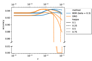
(a) Mean accuracy against $\epsilon$ & $\kappa$

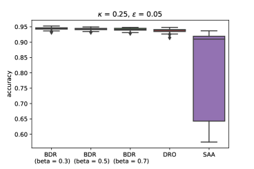
(b) Box plot of accuracy

Figure 2: Average out-of-sample accuracy for 3 vs 8 over 100 independent trials.

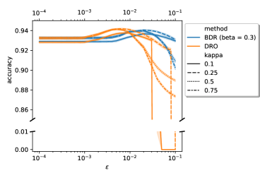
(a) Mean accuracy against $\epsilon$ & $\kappa$

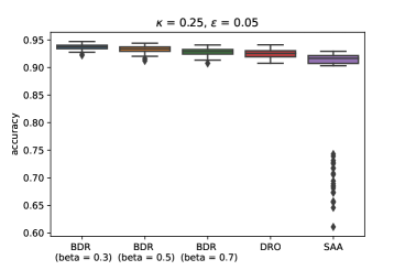
(b) Box plot of accuracy

Figure 3: Average out-of-sample accuracy for 4 vs 9 over 100 independent trials.

References

- Aminian et al. [2021] G. Aminian, Y. Bu, L. Toni, M. Rodrigues, and G. Wornell. An exact characterization of the generalization error for the gibbs algorithm. Advances in Neural Information Processing Systems, 34:8106–8118, 2021.
- Anderson and Nguyen [2020] E. Anderson and H. Nguyen. When can we improve on sample average approximation for stochastic optimization? Operations Research Letters, 48(5):566–572, 2020.
- Ben-Tal et al. [2013] A. Ben-Tal, D. Den Hertog, A. De Waegenaere, B. Melenberg, and G. Rennen. Robust solutions of optimization problems affected by uncertain probabilities. Management Science, 59(2):341–357, 2013.
- Bishop and Nasrabadi [2006] C. M. Bishop and N. M. Nasrabadi. Pattern Recognition and Machine Learning. Springer, 2006.
- Blanchet et al. [2019] J. Blanchet, Y. Kang, and K. Murthy. Robust Wasserstein profile inference and applications to machine learning. Journal of Applied Probability, 56(3):830–857, 2019.
- Blanchet et al. [2021] J. Blanchet, K. Murthy, and V. A. Nguyen. Statistical analysis of Wasserstein distributionally robust estimators. In Tutorials in Operations Research: Emerging Optimization Methods and Modeling Techniques with Applications, pages 227–254. INFORMS, 2021.
- Bousquet and Elisseeff [2002] O. Bousquet and A. Elisseeff. Stability and generalization. The Journal of Machine Learning Research, 2:499–526, 2002.
- Chen et al. [2020] R. Chen, I. C. Paschalidis, et al. Distributionally robust learning. Foundations and Trends® in Optimization, 4(1-2):1–243, 2020.
- Chernick [2011] M. R. Chernick. Bootstrap methods: A Guide for Practitioners and Researchers. John Wiley & Sons, 2011.
- Ferguson [1973] T. S. Ferguson. A Bayesian analysis of some nonparametric problems. The Annals of Statistics, pages 209–230, 1973.
- Fournier and Guillin [2015] N. Fournier and A. Guillin. On the rate of convergence in Wasserstein distance of the empirical measure. Probability Theory and Related Fields, 162(3):707–738, 2015.
- Gao [2022] R. Gao. Finite-sample guarantees for Wasserstein distributionally robust optimization: Breaking the curse of dimensionality. Operations Research, 2022.
- Gao and Kleywegt [2022] R. Gao and A. Kleywegt. Distributionally robust stochastic optimization with Wasserstein distance. Mathematics of Operations Research, 2022.
- Gao et al. [2022] R. Gao, X. Chen, and A. J. Kleywegt. Wasserstein distributionally robust optimization and variation regularization. Operations Research, 2022.
- Gaudard and Hadwin [1989] M. Gaudard and D. Hadwin. Sigma-algebras on spaces of probability measures. Scandinavian Journal of Statistics, pages 169–175, 1989.
- Germain et al. [2016] P. Germain, F. Bach, A. Lacoste, and S. Lacoste-Julien. PAC-Bayesian theory meets Bayesian inference. Advances in Neural Information Processing Systems, 29, 2016.
- Ghosal and Van der Vaart [2017] S. Ghosal and A. Van der Vaart. Fundamentals of Nonparametric Bayesian Inference, volume 44. Cambridge University Press, 2017.
- Goodfellow et al. [2016] I. Goodfellow, Y. Bengio, and A. Courville. Deep Learning. MIT Press, 2016.
- Hastie et al. [2009] T. Hastie, R. Tibshirani, and J. Friedman. The elements of statistical learning: Data mining, inference, and prediction. Springer New York, 2009.
- Kuhn et al. [2019] D. Kuhn, P. M. Esfahani, V. A. Nguyen, and S. Shafieezadeh-Abadeh. Wasserstein distributionally robust optimization: Theory and applications in machine learning. In Operations Research & Management Science in the Age of Analytics, pages 130–166. INFORMS, 2019.
- LeCun [1998] Y. LeCun. The mnist database of handwritten digits. http://yann. lecun. com/exdb/mnist/, 1998.
- Mohajerin Esfahani and Kuhn [2018] P. Mohajerin Esfahani and D. Kuhn. Data-driven distributionally robust optimization using the Wasserstein metric: Performance guarantees and tractable reformulations. Mathematical Programming, 171(1):115–166, 2018.
- Rahimian and Mehrotra [2022] H. Rahimian and S. Mehrotra. Frameworks and results in distributionally robust optimization. Open Journal of Mathematical Optimization, 3:1–85, 2022.
- Rodríguez Gálvez et al. [2021] B. Rodríguez Gálvez, G. Bassi, R. Thobaben, and M. Skoglund. Tighter expected generalization error bounds via Wasserstein distance. Advances in Neural Information Processing Systems, 34:19109–19121, 2021.
- Shafieezadeh-Abadeh et al. [2019] S. Shafieezadeh-Abadeh, D. Kuhn, and P. M. Esfahani. Regularization via mass transportation. Journal of Machine Learning Research, 20(103):1–68, 2019.
- Van der Vaart [2000] A. W. Van der Vaart. Asymptotic Statistics. Cambridge University Press, 2000.
- Vapnik [1998] V. Vapnik. Statistical Learning Theory. Wiley-Interscience, 1998.
- Varoquaux [2018] G. Varoquaux. Cross-validation failure: Small sample sizes lead to large error bars. Neuroimage, 180:68–77, 2018.
- Wainwright [2019] M. J. Wainwright. High-Dimensional Statistics: A Non-Asymptotic Viewpoint, volume 48. Cambridge University Press, 2019.
- Wang et al. [2019] H. Wang, M. Diaz, J. C. S. Santos Filho, and F. P. Calmon. An information-theoretic view of generalization via Wasserstein distance. In 2019 IEEE International Symposium on Information Theory (ISIT), pages 577–581. IEEE, 2019.
- Wang et al. [2022] S. Wang, H. Wang, and J. Honorio. Distributional robustness bounds generalization errors, 2022. URL https://arxiv.org/abs/2212.09962.
- Wu et al. [2018] D. Wu, H. Zhu, and E. Zhou. A Bayesian risk approach to data-driven stochastic optimization: Formulations and asymptotics. SIAM Journal on Optimization, 28(2):1588–1612, 2018.
- Xu and Raginsky [2017] A. Xu and M. Raginsky. Information-theoretic analysis of generalization capability of learning algorithms. Advances in Neural Information Processing Systems, 30, 2017.
- Yue et al. [2021] M.-C. Yue, D. Kuhn, and W. Wiesemann. On linear optimization over Wasserstein balls. Mathematical Programming, pages 1–16, 2021.
- Zhang and Chen [2021] H. Zhang and S. Chen. Concentration inequalities for statistical inference. Communications in Mathematical Research, 37(1):1–85, 2021.