Heat currents in qubit systems

Abstract

There is a current interest in quantum thermodynamics in the context of open quantum systems. An important issue is the consistency of quantum thermodynamics, in particular the second law of thermodynamics, i.e., the flow of heat from a hot reservoir to a cold reservoir. Here recent emphasis has been on composite system and in particular the issue regarding the application of local or global master equations. In order to contribute to this discussion we discuss two cases, namely as an example a single qubit and as a simple composite system two coupled qubits driven by two heat reservoirs at different temperatures, respectively. Applying a global Lindblad master equation approach we present explicit expressions for the heat currents in agreement with the second law of thermodynamics. The analysis is carried out in the Born-Markov approximation. We also discuss issues regarding the possible presence of coherences in the steady state.

I Introduction

There is a current interest in quantum thermodynamics Alicki (1979); Barra (2015); Kosloff (2013); Kosloff and Levy (2014); Mari and Eisert (2012); Kosloff and Levy (2019); Levy et al. (2020); Colla and Breuer (2021); Linden et al. (2010). Thermodynamics is a universal theory and must from a fundamental point of view emerge from a microscopic point of view. In this context the emergence of in particular the second law of thermodynamics. In the Clausius formulation the second law implies that heat flows from a hot reservoir to a cold reservoir and this essential property should also hold in the quantum regime. In non equilibrium quantum statistical mechanics the instantaneous heat current is of course subject to both statistical and quantum fluctuations, however, the mean heat current must obey the second law of thermodynamics.

The natural framework for discussing these issues is the theory of open quantum systems Breuer and Petruccione (2006); Rivas and Huelga (2012); Carmichael (1976). Here the focus is on a small controllable quantum system interacting with an environment which can be either radiation fields or heat baths. In order to obtain a steady heat current we must drive the quantum system by several heat reservoirs, typically two reservoirs, maintained at different temperatures.

Whereas the case of a single qubit (two-level atomic system) driven by two heat bath is easily analysed Aurell and Montana (2019) and discussed in the present paper, the discussion in the literature is usually focussed on composite systems Kohler et al. (2005); Kosloff and Levy (2014). Here a recent discussion has focussed on the connection between a global master equation approach as applied in the present paper and a local master equation approach in which the interactions in the composite system is ignored in the dissipative kernels. It has been shown that in the case of a local master equation approach the apparent violation of the second law can be remedied by using a protocol of repeated interactions; this scheme accounts for a work contribution which together with the heat contribution restores the validity of the second law Barra (2015); Pereira (2018); Chiara et al. (2018); Hewgill et al. (2021). In the case of coupled quantum oscillators driven by two heat reservoirs a global approach was discussed in Levy and Kosloff (2014) resolving the issue regarding the second law.

In the present work, motivated by the study in Levy and Kosloff (2014), we discuss a composite system of two coupled qubits driven by two heat reservoirs. Coupled qubit systems has been studied extensively but mainly in the context of quantum entanglement del Valle (2010); Liao et al. (2011); Fischer and Breuer (2013); Duan et al. (2013); Paneru et al. (2020); Schlosshauer (2019); Aolita et al. (2015); Decordi and Vidiella-Barranco (2017); Bresque et al. (2021); Hewgill et al. (2018); Hu et al. (2018); Karimi et al. (1965); in the present paper, however, the focus is on quantum thermodynamics and the second law of thermodynamics.

In discussing open quantum systems described by a master equation the focus is on the density matrix $\rho_{pp^{\prime}}(t)$, where the index $p$ refers to an energy basis. Here we distinguish between populations characterised by the diagonal density matrix elements $\rho_{nn}(t)$ and coherences described by the off-diagonal matrix elements $\rho_{nm}(t)$, $n\neq m$. For physical reasons the populations must be positive, $\rho_{nn}\geq 0$ and, moreover, satisfy the trace condition $\sum_{n}\rho_{nn}=1$ (conservation of probability). Such a requirement does not apply to the coherences $\rho_{n\neq m}$ which in general are complex numbers. For a single qubit driven by one or several heat reservoirs the coherences do not couple to the populations. The populations settle to their steady state values and the coherences die out. For a composite system the situation is different. Here coherences can in principle couple to populations and influence the steady state.. This is for example the case in Li et al. (2014); Zhang and Wang (2014); Wichterich et al. (2007). Here we address this issue in the case of driven coupled qubits,

It is well-established that the proper master equation to be used in dealing with open quantum systems is the Lindblad form Breuer and Petruccione (2006); Manzano (2020); Lindblad (1976); Chruscinski and Pascazio (2017) which in the Markov limit ensures that the density matrix evolves in time according to a quantum dynamical semigroup defining a so-called quantum channel Wilde (2017). The Lindblad master equation thus ensures that the populations stay positive and that the trace condition $\sum_{n}\rho_{nn}(t)=0$ (conservation of probability) is satisfied. The Redfield master equation Redfield (1965) introduced prior to the Lindblad form preserves the trace but does not represent a quantum channel and can lead to unphysical negative populations; note that the trace condition does not in itself ensure positive populations.

In recent work we applied a field theoretical condensed matter approach to open quantum system Fogedby (2022). Choosing a Caldeira-Leggett multi oscillator heat bath Caldeira and Leggett (1983); Caldeira (1983) and invoking Wick’s theorem we derived a Dyson equation for the transmission operator $T$ propagating the density operator according to $\rho(t)=T(t,0)\rho(0)$. The Dyson equation incorporating secular effects has the schematic form $T=T_{0}+T_{0}KT$, where the kernel $K$ can be determined by a an expansion in powers of the system-bath coupling in terms of Feynman diagrams. Finally, applying a so-called quasi particle approximation, well-known in condensed matter many body theory, we derived a master equation in the Markov approximation. In the field theoretical approach the Dyson equation replaces some of the physical assumptions made in the standard derivation of a master equation. In the Born approximation the field theoretical method basically corresponds to the Redfield equation Redfield (1965); Breuer and Petruccione (2006) in an energy basis. Whereas the trace condition is automatically satisfied, the field theoretical approach does not define a quantum channel, unless a further selection rule is imposed. The selection rule corresponds to the rotating wave approximation used in turning the Redfield equation into the Lindblad equation in the standard derivation Breuer and Petruccione (2006). In more detail, the system operator $S^{\alpha}$ in an energy basis, $S^{\alpha}_{nn^{\prime}}$, appears in a bilinear combination $S^{\alpha}_{nn^{\prime}}S^{\beta}_{pp^{\prime}}$ in both the Redfield and Lindblad cases. As discussed in Fogedby (2022), the selection rule enters as a constraint on the energy transitions according to $S^{\alpha}_{nn^{\prime}}S^{\beta}_{pp^{\prime}}\delta(E_{nn^{\prime}}+E_{pp^{\prime}})$, where $E_{nn^{\prime}}=E_{n}-E_{n^{\prime}}$ is the energy associated with the transition $n\to n^{\prime}$. In a physical interpretation the selection rule implies that the transition energies in the bilinear terms have to match. It is also clear that whether the selection rule imposes a constraint depends on the matrix elements $S^{\alpha}_{nn^{\prime}}$. In cases where the selection rule is trivially satisfied the Redfield and Lindblad approaches yield identical density matrices.

In the present paper we find that a Redfield approach to the case of coupled qubits does yield coherence contribution to the steady state and, moreover, gives rise to unphysical negative populations. In a proper Lindblad approach, corresponding to a quantum channel, the populations are positive and the heat currents are in accordance with the second law of thermodynamics.

The paper is organised as follows. In Sec. II we discuss i) the master equation, ii) the heat currents, and iii) the Redfield - Lindblad approaches and coherences. In Sec. III we consider i) the single qubit case and ii) the coupled-qubit case. In Sec. III.3 we show that a Redfield approach yield unphysical negative populations. In Sec. IV we give a brief discussion and summary. Details regarding the Redfield approach is deferred to Appendix A

II General Analysis

Here we set up the general scheme for the evaluation of the density matrix and heat currents for an open system driven by two heat reservoirs.

II.1 Master equation

The density operator for an open quantum system $S$ characterised by the Hamiltonian $H$ interacting with a single or several heat reservoirs is in the Markov approximation governed by a master equation of the form Breuer and Petruccione (2006); Rivas and Huelga (2012); Fogedby (2022)

$$\frac{d\rho(t)}{dt}=-i[H,\rho(t)]+L\rho(t).$$ (1)

The von Neumann term $-i[H,\rho(t)]$ yields the reversible unitary time evolution von Neumann (1927). The second term driven by the super operator $L$ characterises the coupling to the environment. This term has the structure $L=K+i\Delta$, where $\Delta$ is a Lamb type correction to the energy levels. The dissipative kernel $K$ characterises the relaxation of the system. In the following we assume that the shift $\Delta$ is incorporated in $H$ and focus on the dissipative kernel $K$.

In an energy basis, which we shall use in the following, we have $H|n\rangle=E_{n}|n\rangle$, where $|n\rangle$ denotes the wavefunction and $E_{n}$ the associated energy. Expanding the von Neumann term the master equation in (1) takes the form

$$\frac{d\rho(t)_{pp^{\prime}}}{dt}=-iE_{pp^{\prime}}\rho(t)_{pp^{\prime}}+\sum_{qq^{\prime}}K_{pp^{\prime},qq^{\prime}}\rho(t)_{qq^{\prime}},$$ (2)

where the energy shift is given by $E_{pp^{\prime}}=E_{p}-E_{p^{\prime}}$, the density matrix by $\rho(t)_{pp^{\prime}}=\langle p|\rho(t)|p^{\prime}\rangle$, and the kernel super matrix by $K_{pp^{\prime},qq^{\prime}}=\langle p|\langle q^{\prime}|K|q\rangle|p^{\prime}\rangle$. We are, moreover, in the following assuming that the Markov approximation, i.e., the separation of time scales, applies and that the kernel $K$ is time independent.

Consequently, the steady state density matrix denoted by $\rho_{pp^{\prime}}$ is determined by a set of linear equations

$$-iE_{pp^{\prime}}\rho_{pp^{\prime}}+\sum_{qq^{\prime}}K_{pp^{\prime},qq^{\prime}}\rho_{qq^{\prime}}=0;$$ (3)

note that the trace condition $\sum_{n}\rho_{nn}(t)=1$ implies $\sum_{n}d\rho_{nn}(t)/dt=0$ and thus

$$\sum_{p}K_{pp,qq^{\prime}}=0.$$ (4)

Separating (3) with respect to populations and coherences, respectively, we obtain the coupled linear equations

$$\sum_{q}K_{pp,qq}\rho_{qq}+\sum_{q\neq q^{\prime}}K_{pp,qq^{\prime}}\rho_{qq^{\prime}}=0,$$ (5)

$$-iE_{pp^{\prime}}\rho_{pp^{\prime}}+\sum_{q\neq q^{\prime}}K_{pp^{\prime},qq^{\prime}}\rho_{qq^{\prime}}+\sum_{q}K_{pp^{\prime},qq}\rho_{qq}=0,\text{for}~{}p\neq p^{\prime},$$ (6)

where in (5) the populations $\rho_{qq}$ are coupled to the coherences $\rho_{q\neq q^{\prime}}$ driving the populations in (6). Thus, in order for coherences to influence the population we must have $K_{pp,q\neq q^{\prime}}\neq 0$.

II.2 Currents

The mean energy of the system is given by $E(t)=\text{Tr}(H\rho(t))$. For the energy or heat flux we thus have $q(t)=\text{Tr}(Hd\rho(t)/dt)$ or inserting (3)

$$q=\sum_{n,qq^{\prime}}E_{n}K_{nn,qq^{\prime}}\rho_{qq^{\prime}}.$$ (7)

For a single heat reservoir the system equilibrates and it it follows directly from (3) that the heat current $q$ vanishes. However, in the presence of several heat reservoirs maintained at different temperatures a steady state heat current will be generated.

In the case of two uncorrelated heat reservoirs $A$ and $B$ the kernel $K$ in (3) is composed of two parts associated with each reservoir and we have

$$K_{pp^{\prime},qq^{\prime}}=K_{pp^{\prime},qq^{\prime}}^{A}+K_{pp^{\prime},qq^{\prime}}^{B};$$ (8)

note that in the case where the heat bath are correlated there will an additional term $K_{pp^{\prime},qq^{\prime}}^{A,B}$ depending on both heat baths.

As a result the total current is determined by

$$q=\sum_{n,qq^{\prime}}E_{n}(K_{nn,qq^{\prime}}^{A}+K_{nn,qq^{\prime}}^{B})\rho_{qq^{\prime}}.$$ (9)

The vanishing total current has components associated with each bath, i.e.,

$$q=q^{A}+q^{B}=0,$$ (10)

$$q^{A}=\sum_{n,qq^{\prime}}E_{n}K_{nn,qq^{\prime}}^{A}\rho_{qq^{\prime}},$$ (11)

$$q^{B}=\sum_{n,qq^{\prime}}E_{n}K_{nn,qq^{\prime}}^{B}\rho_{qq^{\prime}}.$$ (12)

We infer that the heat flux from the reservoir $A$ to the system $S$ given by $q^{A}$ equals the heat flux $-q^{B}=q^{A}$ flowing from the system $S$ into the reservoir $B$, expressing energy conservation, i.e. the first law of thermodynamics. Regarding the second law of thermodynamics the issue is to show that a positive heat current flows from the hot heat reservoir to the cold heat reservoir. From the above it follows that in order to evaluate the heat currents for a given open quantum system driven by two reservoirs we need three components: The energy spectrum of the system $E_{n}$, the kernel elements $K^{A,B}_{nn,qq^{\prime}}$, and the density operator $\rho_{qq^{\prime}}$.

II.3 Redfield - Lindblad - Coherences

Then issue of coherences in the steady state and currents is subtle Li et al. (2014); Zhang and Wang (2014); Wichterich et al. (2007). In recent work Fogedby (2022) alluded to in the introduction we presented a detailed discussion of the application of field theoretical methods to open quantum systems. The field theoretical approach is based on a systematic expansion in terms of diagrams and applies a condensed matter quasi-particle approximation in order to implement the Markov limit. The field theoretical method is the basis for the present analysis.

Assuming a system - bath coupling of the form $\sum_{\alpha}S^{\alpha}B^{\alpha}$, where $S^{\alpha}$ are the system operators and $B^{\alpha}$ the bath operators, the dissipative kernel $K_{pp^{\prime},qq^{\prime}}$ in the Born approximation and in an energy basis is given by

$$K^{\text{Red}}_{pp^{\prime},qq^{\prime}}= -\delta_{p^{\prime}q^{\prime}}\frac{1}{2}\sum_{\alpha\beta,l}S^{\alpha}_{pl}S^{\beta}_{lq}D^{\alpha\beta}(E_{pl})-\delta_{pq}\frac{1}{2}\sum_{\alpha\beta,l}S^{\alpha}_{q^{\prime}l}S^{\beta}_{lp^{\prime}}D^{\alpha\beta}(E_{p^{\prime}l})$$ (13)

$$+\frac{1}{2}\sum_{\alpha\beta}S^{\beta}_{pq}S^{\alpha}_{q^{\prime}p^{\prime}}(D^{\alpha\beta}(E_{q^{\prime}p^{\prime}})+D^{\alpha\beta}(E_{qp})).$$

Here $D^{\alpha\beta}(\omega)$ is the bath correlation function given by

$$D^{\alpha\beta}(\omega)=\int dt\exp(i\omega(t-t^{\prime}))\text{Tr}_{B}[\rho_{B}B^{\alpha}(t)B^{\beta}(t^{\prime})],$$ (14)

$$\rho_{B}=\frac{\exp(-H_{B}/T)}{\text{Tr}_{B}[\exp(-H_{B}/T)]},$$ (15)

where $H_{B}=\sum_{k}\omega_{k}b_{k}^{\dagger}b_{k}$ is the bath Hamiltonian, $b_{k}$ the Bose operator associated with the wavenumber $k$, and $T$ the associated temperature.

By inspection of (13) it is easily seen that the trace condition in (4) is satisfied. However, the field theoretical approach which in the Born approximation is equivalent to the Redfield equation Redfield (1965) does not represent the generator of a quantum dynamical semigroup and thus does not guarantee that the populations are positive. In order to implement the semigroup properties and thus guarantee positive populations one must impose a further secular rotating wave approximation (RWA) yielding the Lindblad equation Breuer and Petruccione (2006).

In operator form the Lindblad master equation has the general form

$$\frac{d}{dt}\rho(t)=-i[H,\rho(t)]+\sum_{\alpha\beta,k}\gamma_{k}^{\alpha\beta}\Big{[}S^{\beta}_{k}\rho(t)S_{k}^{\alpha\dagger}-\frac{1}{2}\{S_{k}^{\alpha\dagger}S_{k}^{\beta},\rho(t)\}\Big{]}.$$ (16)

However, as shown in Fogedby (2022) the introduction of the RWA amounts to introducing delta function constraints in the kernel (13) yielding the expression

$$K^{\text{Lind}}_{pp^{\prime},qq^{\prime}}= -\frac{\delta_{p^{\prime}q^{\prime}}}{2}\sum_{\alpha\beta,l}S^{\alpha}_{pl}S^{\beta}_{lq}\delta(E_{pl}+E_{lq})D^{\alpha\beta}(E_{pl})-\frac{\delta_{pq}}{2}\sum_{\alpha\beta,l}S^{\alpha}_{q^{\prime}l}S^{\beta}_{lp^{\prime}}\delta(E_{q^{\prime}l}+E_{lp^{\prime}})D^{\alpha\beta}(E_{p^{\prime}l})$$ (17)

$$+\frac{1}{2}\sum_{\alpha\beta}S^{\beta}_{pq}S^{\alpha}_{q^{\prime}p^{\prime}}\delta(E_{pq}+E_{q^{\prime}p^{\prime}})(D^{\alpha\beta}(E_{q^{\prime}p^{\prime}})+D^{\alpha\beta}(E_{qp})).$$

In the interaction representation the system operator $S^{\alpha}_{pq}(t)\propto\exp(-iE_{pq}t)$. Consequently, the product $S^{\alpha}_{pq}(t)S^{\beta}_{p^{\prime}q^{\prime}}(t)\propto\exp(-i(E_{pq}+E_{p^{\prime}q^{\prime}})t)$. For $E_{pq}+E_{p^{\prime}q^{\prime}}\neq 0$ this term will oscillate and is discarded in the RWA. As a result, whether the delta function constraint eliminates terms in the super operator $K_{pp^{\prime},qq^{\prime}}$ depends on the matrix elements $S^{\alpha}_{pq}$ and thus on the specific model under consideration.

We stress that a proper analysis satisfying the correct physics requires the Lindblad equation. Whether the Lindblad equation then generates coherences in the steady state will, as mentioned above, depend on the specific model Li et al. (2014); Zhang and Wang (2014); Wichterich et al. (2007). In the case of a single driven qubit it follows immediately that coherences are absent in the steady state. In the coupled qubit case we find that a Redfield treatment according to (13) yield coherences in the steady state and unphysical negative populations. On the other hand, for coupled qubits a Lindblad treatment according to (17) yields vanishing coherences, positive populations and simple expressions for the currents.

III Qubit systems driven by two heat reservoirs

In this section we turn to the case of qubit systems driven by two heat reservoirs generating a non equilibrium heat current. As an example and illustration we first consider the case of a driven single qubit. The second case, constituting the main issue in the paper, is a coupled qubit system.

III.1 Single qubit

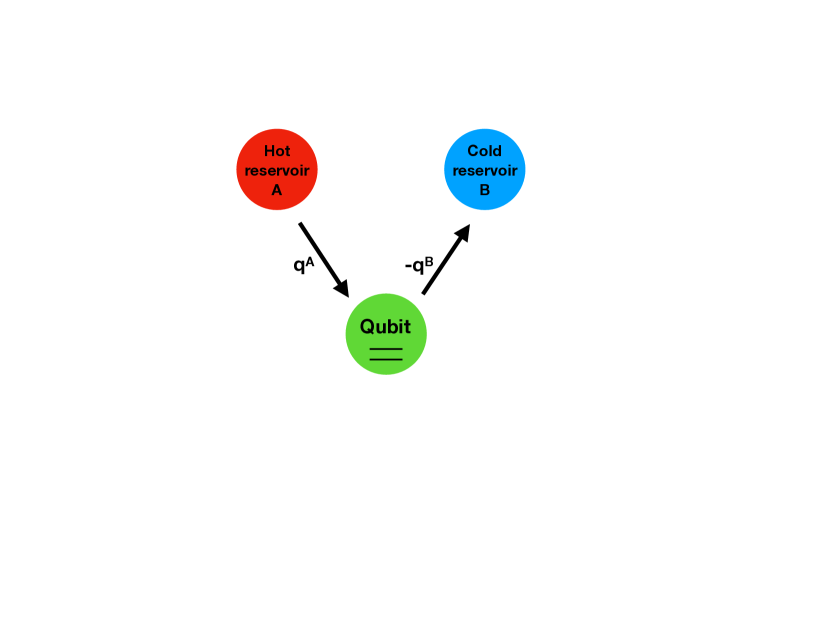
Figure 1: We depict the drive of a single qubit by a hot heat reservoir $A$ and a cold heat reservoir $B$.

Here we consider the case of a single qubit driven by two heat reservoirs $A$ and $B$ maintained at temperatures $T_{A}$ and $T_{B}$, respectively. In this case the energy or heat flows from the hot reservoir to the cold reservoir via the qubit; the configuration is depicted in Fig. 1.

III.1.1 Model

In a Pauli matrix basis Zinn-Justin (1989) the Hamiltonian and the coupling to the reservoirs are given by

$$H=\frac{\omega_{0}}{2}\sigma^{z}$$ (18)

$$H_{A}=\sigma^{+}A+\sigma^{-}A^{\dagger},$$ (19)

$$H_{B}=\sigma^{+}B+\sigma^{-}B^{\dagger},$$ (20)

$$A=\sum_{k}\lambda_{k}^{A}a_{k},$$ (21)

$$B=\sum_{k}\lambda_{k}^{B}b_{k},$$ (22)

where the levels $|+\rangle$ and $|-\rangle$ have energies $E_{+}=\omega_{0}/2$ and $E_{-}=-\omega_{0}/2$, corresponding to the energy splitting $\omega_{0}$. The qubit is driven by two heat reservoirs in the rotating wave approximation (RWA). The bath operators $A$ and $B$ sample the bath modes with wavenumber $k$, frequencies $\omega_{k}^{A,B}$, and strength $\lambda_{k}^{A,B}$; $a_{k}$ and $b_{k}$ are Bose operators.

Referring to Sec. II we choose the assignment $S^{\alpha}=(S^{1},S^{2})=(\sigma^{+},\sigma^{-})$, $A^{\alpha}=(A^{1},A^{2})=(A,A^{\dagger})$, and $B^{\alpha}=(B^{1},B^{2})=(B,B^{\dagger})$. For the bath correlations we find

$$D^{12}_{A,B}(\omega)=g_{A,B}(\omega)(1+n_{A,B}(\omega)),~{}~{}\omega>0,$$ (23)

$$D^{21}_{A,B}(\omega)=g_{A,B}(-\omega)n_{A,B}(-\omega),~{}~{}~{}~{}~{}\omega<0,$$ (24)

with spectral functions and Planck distributions

$$g_{A,B}(\omega)=2\pi\sum_{k}(\lambda_{k}^{A,B})^{2}\delta(\omega-\omega^{A,B}_{k}),$$ (25)

$$n_{A,B}(\omega)=\frac{1}{\exp(\omega/T_{A,B})-1}.$$ (26)

Inserting the nonvanishing matrix elements $\langle+|\sigma^{+}|-\rangle=\langle-|\sigma^{-}|+\rangle=1$ with associated energy shifts $E_{+-}=-E_{-+}=\omega_{0}$ we obtain from (17) with the abbreviations $g_{A,B}=g_{A,B}(\omega_{0})$ and $n_{A,B}=n_{A,B}(\omega_{0})$ the dissipative kernel elements

$$K^{A,B}_{++,++}=-g_{A,B}(1+n_{A,B}),$$ (27)

$$K^{A,B}_{--,++}=+g_{A,B}(1+n_{A,B}),$$ (28)

$$K^{A,B}_{++,--}=+g_{A,B}n_{A,B},$$ (29)

$$K^{A,B}_{--,--}=-g_{A,B}n_{A,B},$$ (30)

$$K^{A,B}_{+-,+-}=-\frac{g_{A,B}}{2}(1+2n_{A,B}),$$ (31)

$$K^{A,B}_{-+,-+}=-\frac{g_{A,B}}{2}(1+2n_{A,B});$$ (32)

we note that the delta function constraints in (17) is trivially satisfied showing that the Redfield and Lindblad schemes yield identical kernel elements. Note also that there is no coupling between populations and coherences, i.e. $K_{nn,q\neq q^{\prime}}=0$.

III.1.2 Density matrix

Expressing the kernel $K$ in matrix form

$$K=\left(\begin{array}[]{cccc}K_{++,++}&K_{++,--}&0&0\\ K_{--,++}&K_{--,--}&0&0\\ 0&0&K_{+-,+-}&0\\ 0&0&0&K_{-+,-+}\end{array}\right),$$ (37)

we have (suppressing indices)

$$K=\left(\begin{array}[]{cccc}-g(1+n)&gn&0&0\\ g(1+n)&-gn&0&0\\ 0&0&-(g/2)(1+2n)&0\\ 0&0&0&-(g/2)(1+2n)\end{array}\right),$$ (42)

forming a ”population” block $P$ and a ”coherence” block $C$. For the determinant of $K$ we thus have $\det K=\det P\det C$, where $\det P=0$ and $\det C=(g(1+2n))^{2}/4\neq 0$. Consequently, the populations $\rho_{nn}$ determined by the linear equations $P\rho=0$, requiring a vanishing determinant, yield finite populations, whereas the coherences determined by $C\rho=0$ vanish in the steady state since the determinant is non vanishing. Applying the scheme in Sec. II we readily obtain the populations or diagonal density matrix elements

$$\rho_{++}=\frac{g_{A}n_{A}+g_{B}n_{B}}{g_{A}(1+2n_{A})+g_{B}(1+2n_{B})},$$ (43)

$$\rho_{--}=\frac{g_{A}(1+n_{A})+g_{B}(1+n_{B})}{g_{A}(1+2n_{A})+g_{B}(1+2n_{B})}.$$ (44)

A few comments regarding the density matrix. Introducing the ratio $r=\rho_{++}/\rho_{--}$ we have from (43) and (44)

$$r=\frac{g_{A}n_{A}+g_{B}n_{B}}{g_{A}(1+n_{A})+g_{B}(1+n_{B})}.$$ (45)

In general the ratio $r$ depends on both the spectral densities $g_{A,B}$, i.e., the structure of the reservoirs, and the temperatures $T_{A,B}$. Turning off for example reservoir $B$ by setting $g_{B}=0$ we obtain the well-studied case of a single qubit driven by a single reservoir Breuer and Petruccione (2006). The ratio $r$ does not depend on the spectral strength and we obtain $r=\exp(-\omega_{0}/T_{A})$, i.e., the Boltzmann distribution. For identical reservoirs with the same spectral densities, i.e., $g_{A}=g_{B}=g$, we obtain $r=(n_{A}+n_{B})/(2+n_{A}+n_{B})$. At high temperatures $r\to 1-\omega_{0}/T$, where $T=(T_{A}+T_{B})/2$ is the mean temperature of the combined reservoirs and the energy levels become equally populated. In the low temperature limit $r\to(\exp(-\omega_{0}/T_{A})+\exp(-\omega_{0}/T_{B}))/2$. Introducing the temperature bias $\Delta=T_{A}-T_{B}$ we have $r\to\exp(-\omega_{0}/T)\cosh(2\omega_{0}/\Delta)$, i.e., a correction to the Boltzmann factor. At high temperature, $T\gg\omega_{0}$, we have $\rho_{+}\to 1/2$ and $\rho_{-}\to 1/2$, i.e., equal populations; at low temperature, $T\ll\omega_{0}$, we have $\rho_{+}\to 0$ and $\rho_{-}\to 1$, i.e., population of the lowest level (ground state).

III.1.3 Currents

Noting that $E_{+}=\omega_{0}/2$ and $E_{-}=-\omega_{0}/2$ the scheme in Sec. II likewise yields expressions for the currents. The steady state heat currents from reservoir $A$ and from reservoir $B$ to the qubit are thus given by

$$q^{A}=\frac{g_{A}g_{B}\omega_{0}}{g_{A}(1+2n_{A})+g_{B}(1+2n_{B})}[n_{A}-n_{B}],$$ (46)

$$q^{B}=\frac{g_{A}g_{B}\omega_{0}}{g_{A}(1+2n_{A})+g_{B}(1+2n_{B})}[n_{B}-n_{A}].$$ (47)

First we note that by construction $q^{A}+q^{B}=0$ showing that energy is conserved, i.e., the first law of thermodynamics. Secondly, since $n_{A}>n_{B}$ for $T_{A}>T_{B}$ energy flows from the hot heat reservoir with temperature $T_{A}$ to the cold heat reservoir maintained at temperature $T_{B}$, demonstrating that the second law of thermodynamics holds.

Regarding the currents given by (46) and (47) we note that they depend on both spectral representations $g^{A}$ and $g^{B}$. Removing for example reservoir $B$ by setting $g^{B}=0$ the currents vanish and the qubit coupled only to reservoir $A$ equilibrates with temperature $T_{A}$. In the high temperature limit for $T_{A,B}\gg\omega_{0}$ we obtain expanding (46) and (47) the classical results

$$q^{A}\sim\frac{1}{2}\frac{g_{A}g_{B}\omega_{0}}{g_{A}T_{A}+g_{B}T_{B}}[T_{A}-T_{B}],$$ (48)

$$q^{B}\sim\frac{1}{2}\frac{g_{A}g_{B}\omega_{0}}{g_{A}T_{A}+g_{B}T_{B}}[T_{B}-T_{A}],$$ (49)

at low temperatures for $T_{A,B}\ll\omega_{0}$ the vanishing currents

$$q^{A}\sim\frac{g_{A}g_{B}\omega_{0}}{g_{A}+g_{B}}\Big{[}e^{-\omega_{0}/T_{A}}-e^{-\omega_{0}/T_{B}}\Big{]},$$ (50)

$$q^{B}\sim\frac{g_{A}g_{B}\omega_{0}}{g_{A}+g_{B}}\Big{[}e^{-\omega_{0}/T_{B}}-e^{-\omega_{0}/T_{A}}\Big{]}.$$ (51)

III.2 Coupled qubits

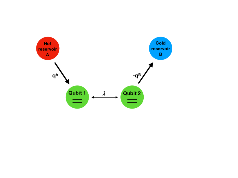
Figure 2: We depict the drive of a composite two-qubit system by a hot heat reservoir $A$ coupled to qubit 1 and a cold heat reservoir $B$ coupled to qubit 2.

This is the main section in the paper. We discuss in detail the case of two coupled qubits driven by two reservoirs as a model of a simple composite system. Heat reservoir $A$ drives qubit 1 and heat reservoir $B$ drives qubit 2. In this case heat flows between the reservoirs and the qubits transmitted across the system by the qubit coupling; the configuration is depicted in Fig. 2.

III.2.1 Model

In a Pauli matrix basis Zinn-Justin (1989) the Hamiltonian and coupling to the reservoirs are given by

$$H=\frac{\omega_{1}}{2}\sigma^{z}_{1}+\frac{\omega_{2}}{2}\sigma^{z}_{2}+\lambda(\sigma^{+}_{1}\sigma^{-}_{2}+\sigma^{-}_{1}\sigma^{+}_{2}).$$ (52)

$$H_{A}=\sigma_{1}^{+}A+\sigma_{1}^{-}A^{\dagger},$$ (53)

$$H_{B}=\sigma_{2}^{+}B+\sigma_{2}^{-}B^{\dagger},$$ (54)

where $\omega_{1}$ and $\omega_{2}$ are the energy splittings of the unperturbed qubits and $\lambda$ the coupling strength of the flip-flop interaction, i.e., the dipole coupling in the RWA. For the composite system we have the unperturbed states $|--\rangle$, $|-+\rangle$, $|+-\rangle$ and $|++\rangle$ with energies $-\omega_{m}$, $-\Delta\omega$, $\Delta\omega$, and $\omega_{m}$, respectively, where

$$\omega_{m}=\frac{\omega_{1}+\omega_{2}}{2},$$ (55)

$$\Delta\omega=\frac{\omega_{1}-\omega_{2}}{2}.$$ (56)

Diagonalising $H$ yields the four states

$$|1\rangle=|--\rangle,$$ (57)

$$|2\rangle=-\beta|+-\rangle+\alpha|-+\rangle,$$ (58)

$$|3\rangle=\alpha|+-\rangle+\beta|-+\rangle,$$ (59)

$$|4\rangle=|++\rangle,$$ (60)

with energies

$$E_{1}=-\omega_{m},$$ (61)

$$E_{2}=-\sqrt{(\Delta\omega)^{2}+\lambda^{2}},$$ (62)

$$E_{3}=\sqrt{(\Delta\omega)^{2}+\lambda^{2}},$$ (63)

$$E_{4}=\omega_{m}.$$ (64)

The expansion coefficients and relevant energy shifts $\omega_{+}=E_{42}=E_{31}$ and $\omega_{-}=E_{43}=E_{21}$ are given by

$$\alpha=\cos\theta/2,$$ (65)

$$\beta=\sin\theta/2,$$ (66)

$$\tan\theta=2\lambda/(\omega_{1}-\omega_{2}),~{}~{}0<\theta<\pi/2,$$ (67)

$$\omega_{+}=\omega_{m}+\sqrt{(\Delta\omega)^{2}+\lambda^{2}},$$ (68)

$$\omega_{-}=\omega_{m}-\sqrt{(\Delta\omega)^{2}+\lambda^{2}}.$$ (69)

For vanishing coupling between the qubits, $\lambda\to 0$, we have $\alpha\to 1$, $\beta\to 0$, $\omega_{+}\to\omega_{1}$, and $\omega_{-}\to\omega_{2}$; moreover, assuming $\omega_{\pm}>0$ we require $\lambda<\sqrt{\omega_{1}\omega_{2}}$.

III.2.2 Kernel

In order to evaluate the dissipative kernel according to the scheme in Sec. II we require the matrix elements of the system operators $\sigma_{1,2}^{\pm}$ in the energy basis $|n\rangle$, $n=1\cdots 4$ of the system Hamiltonian $H$ in (52). With the notation $(\sigma_{1,2}^{\pm})_{pq}=\langle p|\sigma_{1,2}^{\pm}|q\rangle$ we find the non-vanishing matrix elements and associated energy transitions

$$\left(\begin{array}[]{cc}(\sigma^{+}_{1})_{31}&E_{31}\\ (\sigma^{+}_{1})_{42}&E_{42}\\ (\sigma^{+}_{1})_{43}&E_{43}\\ (\sigma^{+}_{1})_{21}&E_{21}\end{array}\right)=\left(\begin{array}[]{cc}\alpha&\omega_{+}\\ \alpha&\omega_{+}\\ \beta&\omega_{-}\\ -\beta&\omega_{-}\end{array}\right),$$ (78)

and

$$\left(\begin{array}[]{cc}(\sigma^{+}_{2})_{21}&E_{21}\\ (\sigma^{+}_{2})_{43}&E_{43}\\ (\sigma^{+}_{2})_{31}&E_{31}\\ (\sigma^{+}_{2})_{42}&E_{42}\end{array}\right)=\left(\begin{array}[]{cc}\alpha&\omega_{-}\\ \alpha&\omega_{-}\\ \beta&\omega_{+}\\ -\beta&\omega_{+}\end{array}\right).$$ (87)

We note that reservoir $A$ drives the $\sigma_{1}$ transitions, whereas reservoir $B$ drives the $\sigma_{2}$ transitions. Moreover, the system operators only appear in the combinations $\sigma_{1}^{+}\sigma_{1}^{-}$ and $\sigma_{2}^{+}\sigma_{2}^{-}$ in the kernel. We also note that the transitions fall in two groups. The transitions $1\leftrightarrow 3$ and $2\leftrightarrow 4$ are associated with $\omega_{+}$, whereas the transitions $1\leftrightarrow 2$ and $3\leftrightarrow 4$ are associated with $\omega_{-}$.

In order to identify nonvanishing kernel elements we inspect the expressions (13) in the Redfield case and (17) in the Lindblad case. We introduce the positive parameters $a_{n},b_{n}$ depending on the coupling strength, spectral densities, Planck distributions and temperatures according to the scheme

$$\left(\begin{array}[]{cc}a_{1}&b_{1}\\ a_{2}&b_{2}\\ a_{3}&b_{3}\\ a_{4}&b_{4}\end{array}\right)=\left(\begin{array}[]{cc}\alpha^{2}g_{A}(\omega_{+})(1+n_{A}(\omega_{+}))&\beta^{2}g_{B}(\omega_{+})(1+n_{B}(\omega_{+}))\\ \beta^{2}g_{A}(\omega_{-})(1+n_{A}(\omega_{-}))&\alpha^{2}g_{B}(\omega_{-})(1+n_{B}(\omega_{-}))\\ \alpha^{2}g_{A}(\omega_{+})n_{A}(\omega_{+})&\beta^{2}g_{B}(\omega_{+})n_{B}(\omega_{+})\\ \beta^{2}g_{A}(\omega_{-})n_{A}(\omega_{-})&\alpha^{2}g_{B}(\omega_{-})n_{B}(\omega_{-})\end{array}\right).$$ (96)

Using the assignment

$$K=\left(\begin{array}[]{cccc}K_{11,11}&K_{11,22}&K_{11,33}&K_{11,44}\\ K_{22,11}&K_{22,22}&K_{22,33}&K_{22,44}\\ K_{33,11}&K_{33,22}&K_{33,33}&K_{33,44}\\ K_{44,11}&K_{44,22}&K_{44,33}&K_{44,44}\end{array}\right),$$

we obtain, since the delta function constraints are trivially satisfied, in both the Redfield and Lindblad cases the kernels $K^{A}$ and $K^{B}$:

$$K^{A}=\left(\begin{array}[]{cccc}-(a_{3}+a_{4})&a_{2}&a_{1}&0\\ a_{4}&-(a_{2}+a_{3})&0&a_{1}\\ a_{3}&0&-(a_{1}+a_{4})&a_{2}\\ 0&a_{3}&a_{4}&-(a_{1}+a_{2})\end{array}\right),$$ (105)

and

$$K^{B}=\left(\begin{array}[]{cccc}-(b_{3}+b_{4})&b_{2}&b_{1}&0\\ b_{4}&-(b_{2}+b_{3})&0&b_{1}\\ b_{3}&0&-(b_{1}+b_{4})&b_{2}\\ 0&b_{3}&b_{4}&-(b_{1}+b_{2})\end{array}\right).$$ (110)

In the Lindblad case, due to the delta function constraints, the above expressions for $K^{A,B}$, yielding populations and currents, exhaust the class of non vanishing kernel elements.

In the Redfield case, relaxing the delta function selection rules, we find non vanishing expressions for kernel elements of the form $K^{A,B}_{pp,q\neq q^{\prime}}$, $K^{A,B}_{p\neq p^{\prime},qq}$, and $K^{A,B}_{p\neq p^{\prime},q\neq q^{\prime}}$ indicating that the populations couple to the coherences. The Redfield case will be discussed in the next section. However, since the Lindblad equation represent a proper quantum channel we proceed with the evaluation of populations and currents.

III.2.3 Density matrix

Introducing the total kernel $K=K^{A}+K^{B}$, where $K^{A}$ and $K^{B}$ are given by (105) and (110), respectively, the populations $\rho_{nn}$ are determined by the linear equations $\sum_{q}K_{pp,qq}\rho_{qq}=0$. By inspection we note incidently that $\det K=0$ allowing for a solution. In terms of the parameters $s_{n}=a_{n}+b_{n}$, $n=1\cdots 4$, where $a_{n},b_{n}$ are given (96), we find the normalised populations, i.e., $\sum_{n}\rho_{nn}=1$,

$$\left(\begin{array}[]{c}\rho_{11}\\ \rho_{22}\\ \rho_{33}\\ \rho_{44}\end{array}\right)=\frac{1}{(s_{1}+s_{3})(s_{2}+s_{4})}\left(\begin{array}[]{c}s_{1}s_{2}\\ s_{1}s_{4}\\ s_{3}s_{2}\\ s_{3}s_{4}\end{array}\right),~{}~{}s_{n}=a_{n}+b_{n}.$$ (119)

In the high temperature limit $T_{A},T_{B}\gg\omega_{+},\omega_{-}$ we have $n_{A,B}(\omega_{\pm})\to T_{A,B}/\omega_{\pm}$ and a simple calculation yields $\rho_{nn}\to 1/4$, i.e., equal population of the four energy levels. Likewise, for $T_{A},T_{B}\ll\omega_{+},\omega_{-}$ we have $\rho_{11}\to 1$ and $\rho_{22},\rho_{33},\rho_{44}\to 0$, i.e., occupation of the lowest energy level.

Finally, for $\lambda=0$ we have $\omega_{+}\to\omega_{1}$, $\omega_{-}\to\omega_{2}$, $s_{1}=a_{1},s_{2}=b_{2},s_{3}=a_{3},s_{4}=b_{4}$ and the populations take the form

$$\left(\begin{array}[]{c}\rho_{11}\\ \rho_{22}\\ \rho_{33}\\ \rho_{44}\end{array}\right)=\frac{1}{(a_{1}+a_{3})(b_{2}+b_{4})}\left(\begin{array}[]{c}a_{1}b_{2}\\ a_{1}b_{4}\\ a_{3}b_{2}\\ a_{3}b_{4}\end{array}\right).$$ (128)

By inspection we conclude that the qubits decouple and we obtain for the density operator the direct product $\rho=\rho^{A}\otimes\rho^{B}$, where

$$\rho^{A}=\frac{1}{g_{A}(\omega_{1})(1+2n_{A}(\omega_{1}))}\left(\begin{array}[]{cc}g_{A}(\omega_{1})(1+n_{A}(\omega_{1}))&0\\ 0&g_{A}(\omega_{1})n_{A}(\omega_{1})\end{array}\right),$$ (131)

and

$$\rho^{B}=\frac{1}{g_{B}(\omega_{2})(1+2n_{B}(\omega_{2}))}\left(\begin{array}[]{cc}g_{B}(\omega_{2})(1+n_{B}(\omega_{2}))&0\\ 0&g_{B}(\omega_{2})n_{B}(\omega_{2})\end{array}\right),$$ (134)

are the equilibrium density operators for qubit 1 coupled to reservoir $A$ and qubit 2 coupled to reservoir $B$, respectively.

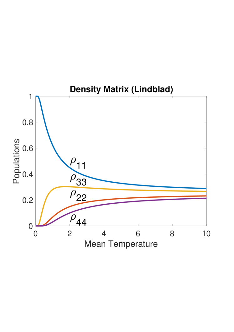
Figure 3: We depict the populations $\rho_{11}$, $\rho_{22}$, $\rho_{33}$, $\rho_{44}$ in the Lindblad case as a function of the mean temperature $T$.

In order to illustrate the Lindblad case we have in Fig. 3 depicted the populations $\rho_{nn}$ as a function of the mean temperature $T=(T_{A}+T_{B})/2$ for $T_{A}=T_{B}$, i.e. in the equilibrium case, with parameter choice $\omega_{1}=1.0$, $\omega_{2}=2.0$, $g_{A}(\omega_{\pm})=g_{B}(\omega_{\pm})=1.0$, and $\lambda=0.5$. For $T=0$ the system occupies the lowest level, i.e., $\rho_{11}=0$; at high temperatures the populations converge, i.e., equal populations, $\rho_{nn}\to 1/4$.

III.2.4 Currents

Applying the scheme in Sec. II the heat currents $q^{A}$ and $q^{b}$ are given by $q^{A}=\sum_{n}E_{n}K^{A}_{nn,pp}\rho_{pp}$ and $q^{B}=\sum_{n}E_{n}K^{B}_{nn,pp}\rho_{pp}$ and we obtain the expressions

$$q^{A}=\frac{a_{3}b_{1}-a_{1}b_{3}}{s_{1}+s_{3}}\omega_{+}+\frac{a_{4}b_{2}-a_{2}b_{4}}{s_{2}+s_{4}}\omega_{-},$$ (135)

$$q^{B}=\frac{a_{1}b_{3}-a_{3}b_{1}}{s_{1}+s_{3}}\omega_{+}+\frac{a_{2}b_{4}-a_{4}b_{2}}{s_{2}+s_{4}}\omega_{-},$$ (136)

or by insertion of $a_{n},b_{n},s_{n}$

$$q^{A}=q^{A}_{+}+q^{A}_{-},$$ (137)

$$q^{A}_{+}=\frac{(\alpha\beta)^{2}g_{A}(\omega_{+})g_{B}(\omega_{+})\omega_{+}}{\alpha^{2}g_{A}(\omega_{+})(1+2n_{A}(\omega_{+}))+\beta^{2}g_{B}(\omega_{+})(1+2n_{B}(\omega_{+}))}[n_{A}(\omega_{+})-n_{B}(\omega_{+})],$$ (138)

$$q^{A}_{-}=\frac{(\alpha\beta)^{2}g_{A}(\omega_{-})g_{B}(\omega_{-})\omega_{-}}{\beta^{2}g_{A}(\omega_{-})(1+2n_{A}(\omega_{-}))+\alpha^{2}g_{B}(\omega_{-})(1+2n_{B}(\omega_{-}))}[n_{A}(\omega_{-})-n_{B}(\omega_{-})].$$ (139)

and

$$q^{B}=q^{B}_{+}+q^{B}_{-},$$ (140)

$$q^{B}_{+}=\frac{(\alpha\beta)^{2}g_{A}(\omega_{+})g_{B}(\omega_{+})\omega_{+}}{\alpha^{2}g_{A}(\omega_{+})(1+2n_{A}(\omega_{+}))+\beta^{2}g_{B}(\omega_{+})(1+2n_{B}(\omega_{+}))}[n_{B}(\omega_{+})-n_{A}(\omega_{+})],$$ (141)

$$q^{B}_{-}=\frac{(\alpha\beta)^{2}g_{A}(\omega_{-})g_{B}(\omega_{-})\omega_{-}}{\beta^{2}g_{A}(\omega_{-})(1+2n_{A}(\omega_{-}))+\alpha^{2}g_{B}(\omega_{-})(1+2n_{B}(\omega_{-}))}[n_{B}(\omega_{-})-n_{A}(\omega_{-})].$$ (142)

By inspection we have $q_{A}+q_{B}=0$ expressing energy conservation, i.e., the first law of thermodynamics. Moreover, and more importantly, since $n_{A}(\omega_{\pm})>n_{B}(\omega_{\pm})$ for $T_{A}>T_{B}$ the current expressions are in accordance with the second law of thermodynamics, i.e., heat flows from the hot reservoir to the cold reservoir; this result corroborates the analysis in Levy and Kosloff (2014) in the case of coupled oscillators driven by two reservoirs.

The heat currents $q^{A}$ and $q^{B}$ in (137 - 142) fall in two parts associated with the energy shifts $\omega_{+}$ and $\omega_{-}$. For vanishing coupling, $\lambda=0$, we have $\alpha=1$ and $\beta=1$, the qubits are uncoupled and the currents vanish. Likewise, quenching e.g. reservoir $B$ by setting $g_{B}=0$ we obtain a vanishing current. In the high temperature limit for $T_{A},T_{B}\gg\omega_{+},\omega_{-}$ we have the classical results

$$q^{A}_{+}=\frac{1}{2}\frac{(\alpha\beta)^{2}g_{A}(\omega_{+})g_{B}(\omega_{+})\omega_{+}}{\alpha^{2}g_{A}(\omega_{+})T_{A}+\beta^{2}g_{B}(\omega_{+})T_{B}}[T_{A}-T_{B}],$$ (143)

$$q^{A}_{-}=\frac{1}{2}\frac{(\alpha\beta)^{2}g_{A}(\omega_{-})g_{B}(\omega_{-})\omega_{-}}{\beta^{2}g_{A}(\omega_{-})T_{A}+\alpha^{2}g_{B}(\omega_{-})T_{B}}[T_{A}-T_{B}].$$ (144)

and

$$q^{B}_{+}=\frac{1}{2}\frac{(\alpha\beta)^{2}g_{A}(\omega_{+})g_{B}(\omega_{+})\omega_{+}}{\alpha^{2}g_{A}(\omega_{+})T_{A}+\beta^{2}g_{B}(\omega_{+})T_{B}}[T_{B}-T_{A}],$$ (145)

$$q^{B}_{-}=\frac{1}{2}\frac{(\alpha\beta)^{2}g_{A}(\omega_{-})g_{B}(\omega_{-})\omega_{-}}{\beta^{2}g_{A}(\omega_{-})T_{A}+\alpha^{2}g_{B}(\omega_{-})T_{B}}[T_{B}-T_{A}].$$ (146)

At low temperatures $T_{A},T_{B}\ll\omega_{+},\omega_{-}$,

$$q^{A}_{+}=\frac{(\alpha\beta)^{2}g_{A}(\omega_{+})g_{B}(\omega_{+})\omega_{+}}{\alpha^{2}g_{A}(\omega_{+})+\beta^{2}g_{B}(\omega_{+})}[e^{-\omega_{+}/T_{A}}-e^{-\omega_{+}/T_{B}}],$$ (147)

$$q^{A}_{-}=\frac{(\alpha\beta)^{2}g_{A}(\omega_{-})g_{B}(\omega_{-})\omega_{-}}{\beta^{2}g_{A}(\omega_{-})+\alpha^{2}g_{B}(\omega_{-})}[e^{-\omega_{-}/T_{A}}-e^{-\omega_{-}/T_{B}}].$$ (148)

and

$$q^{B}_{+}=\frac{(\alpha\beta)^{2}g_{A}(\omega_{+})g_{B}(\omega_{+})\omega_{+}}{\alpha^{2}g_{A}(\omega_{+})+\beta^{2}g_{B}(\omega_{+})}\Big{[}e^{-\omega_{+}/T_{B}}-e^{-\omega_{+}/T_{A}}\Big{]},$$ (149)

$$q^{B}_{-}=\frac{(\alpha\beta)^{2}g_{A}(\omega_{-})g_{B}(\omega_{-})\omega_{-}}{\beta^{2}g_{A}(\omega_{-})+\alpha^{2}g_{B}(\omega_{-})}\Big{[}e^{-\omega_{-}/T_{B}}-e^{-\omega_{-}/T_{A}}\Big{]}.$$ (150)

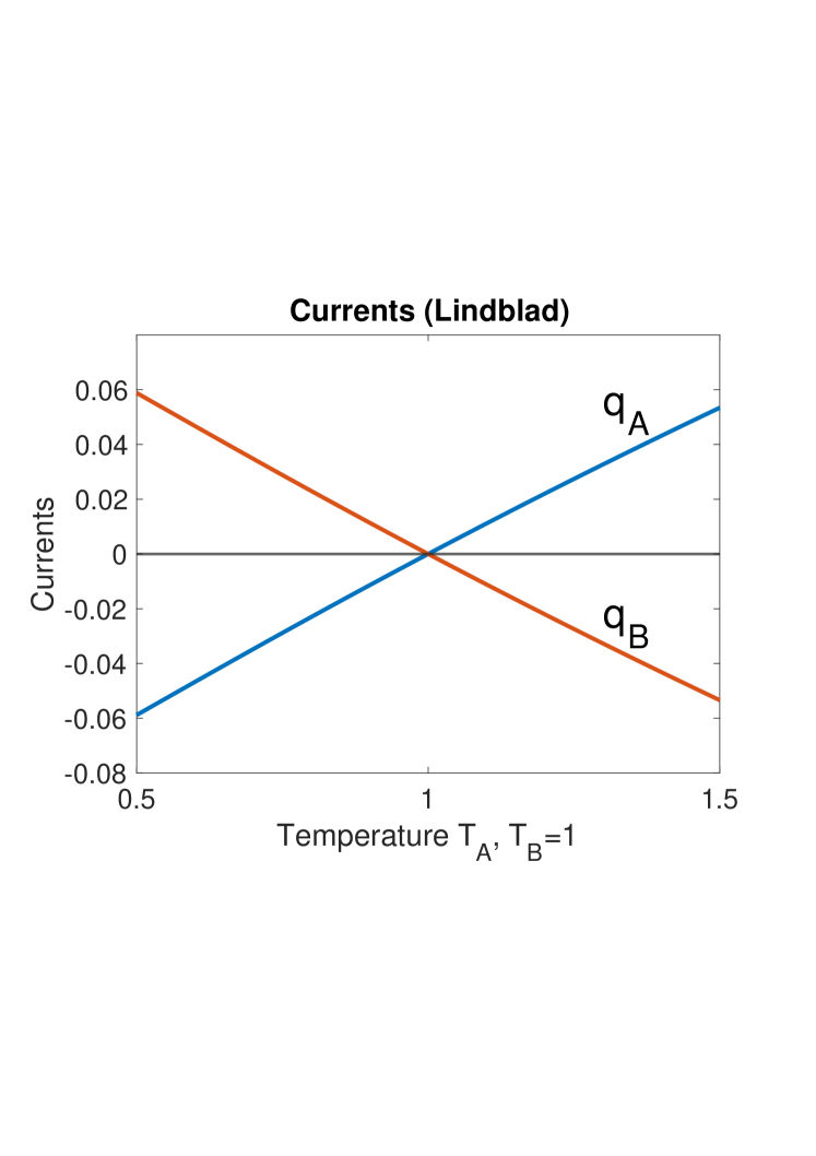
Figure 4: We depict the heat currents $q_{A}$ and $q_{B}$ as functions of $T_{A}$ for $T_{B}=1$.

In Fig. 4 we have depicted the currents $q_{A}$ and $q_{B}$ as a function of $T_{A}$ in the range $0.5$ to $1.5$ with $T_{B}=1$, with parameter choice $\omega_{1}=1.0$, $\omega_{2}=2.0$, $g_{A}(\omega_{\pm})=g_{b}(\omega_{\pm})=1$, and $\lambda=0.5$; note that the currents vanish in equilibrium for $T_{A}=T_{B}$.

III.3 Redfield approach

In this section we discuss briefly the Redfield approach to the coupled qubit system. Relaxing the delta function constraint or selection rule yielding the Lindblad equation it follows from Sec. II that the kernel elements $K^{A,B}_{nn,23},K^{A,B}_{nn,32},K^{A,B}_{23,nn},K^{A,B}_{32,nn}$ for $n=1,4$ and $K^{A,B}_{23,23},K^{A,B}_{32,32}$ are non vanishing indicating that the populations $\rho_{nn}$ couple to the coherences $\rho_{n\neq n^{\prime}}$. The calculation is deferred to Appendix A.

Considering the case $g_{A,B}(\omega_{\pm})=g$ we find the populations and coherences

$$\left(\begin{array}[]{c}\rho_{11}\\ \rho_{22}\\ \rho_{33}\\ \rho_{44}\end{array}\right)=\frac{s^{2}+4e^{2}}{N}\left(\begin{array}[]{c}s_{1}s_{2}\\ s_{1}s_{4}\\ s_{3}s_{2}\\ s_{3}s_{4}\end{array}\right)-\frac{4k^{2}}{N}\left(\begin{array}[]{c}(s_{1}+s_{4})(s_{2}+s_{3})\\ (s_{1}+s_{4})(s_{1}+s_{4})\\ (s_{2}+s_{3})(s_{2}+s_{3})\\ (s_{1}+s_{4})(s_{2}+s_{3})\end{array}\right),$$ (163)

and

$$\left(\begin{array}[]{c}\rho_{23}\\ \rho_{32}\end{array}\right)=-\frac{2k}{N}\left(\begin{array}[]{c}(s_{1}s_{2}-s_{3}s_{4})(s-2ie)\\ (s_{1}s_{2}-s_{3}s_{4})(s+2ie)\end{array}\right).$$ (168)

The trace condition $\sum_{n}\rho_{nn}=1$ yields the normalisation factor

$$N=(s^{2}+4e^{2})(s_{1}+s_{3})(s_{2}+s_{4})-4(ks)^{2}$$ (169)

and we have, moreover, introduced the parameters

$$s=s_{1}+s_{2}+s_{3}+s_{4},$$ (170)

$$e=E_{23}=-E_{32},$$ (171)

$$k=\frac{\alpha\beta g}{2}[n_{A}(\omega_{+})-n_{B}(\omega_{+})+n_{A}(\omega_{-})-n_{B}(\omega_{-})].$$ (172)

In equilibrium $T_{A}=T_{B}$ we have $k=0$. The populations are decoupled from the coherences and the Redfield and Lindblad expression for the populations are in agreement. In the non equilibrium case for $T_{A}\neq T_{B}$ we have $k\neq 0$ and the populations are reduced due to the coherences. The coherences $\rho_{23}$ and $\rho_{32}$ are complex conjugate (the density matrix is hermitian) and their sign depends on $k\propto(n_{A}(\omega_{\pm})-n_{B}(\omega_{\pm}))$, i.e., the sign of $T_{A}-T_{B}$.

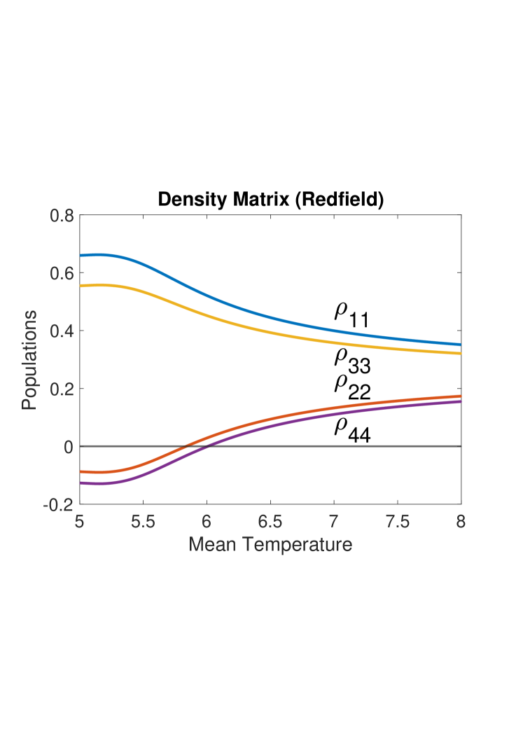
Figure 5: We depict the populations $\rho_{11}$, $\rho_{22}$, $\rho_{33}$, $\rho_{44}$ in the Redfield case as a function of the mean temperature $T$ for $\Delta T=5$ The populations $\rho_{22}$ and $\rho_{44}$ are negative in the range $\Delta T<T\lesssim 6$.

We have in Fig. 5 we have depicted the populations $\rho_{nn}$ as a function of the mean temperature $T=(T_{A}+T_{B})/2$ in the range $\Delta T<T<8$ with non equilibrium bias $\Delta T=(T_{A}-T_{B})/2=5.0$ with parameter choice $\omega_{1}=1.0$, $\omega_{2}=2.0$, $g_{A}(\omega_{\pm})=g_{b}(\omega_{\pm})=1.0$, and $\lambda=0.5$. The plot shows that $\rho_{44}$ and $\rho_{44}$ assumes negative value in the range $0<T\lesssim 6.0$, indicating that the Redfield approach is inadequate in analysing the coupled qubit case.

IV Discussion and summary

In this paper we have discussed heat currents in two qubit systems driven by two heat reservoirs maintained at different temperatures in order to test the validity of the second law of thermodynamics in the microscopic domain, an important issue in quantum thermodynamics. The results for a single qubit system driven by two reservoirs is given in Sec. III.1 and is in accordance with the second law. The case of coupled qubits is more involved, the results are presented in Sec. III.2 and are likewise in agreement with the second law. We note that the current expressions in the single qubit and coupled qubit cases have a similar structure. In deriving these results it is essential to apply a global approach and operate in the basis of the full system Hamiltonian. Moreover, in order to avoid an erroneous result it is also essential to use the Lindblad master equation approach and in this way ensure a proper quantum channel with positive populations.

In order to discuss the possible role of coherences, we made use of a recent field theoretical approach to open quantum system. This method yields at a first stage the Redfield master equation and has to be supplemented with a selection rule in order to produce the Lindblad master equation. The Redfield equation applied directly to the coupled qubit case gives rise to a coupling between coherences and populations in the density matrix but yields negative populations and is thus inadequate is describing the proper physics. *

Appendix A The Redfield case

Here we give details of the Redfield approach to the coupled qubit case. In the following we assume identical reservoirs regarding their structure and define $g=g_{A,B}(\omega_{\pm})$. We introduce the parameters $c_{n},d_{n}$ according to the scheme

$$\left(\begin{array}[]{cc}c_{1}&d_{1}\\ c_{2}&d_{2}\\ c_{3}&d_{3}\\ c_{4}&d_{4}\end{array}\right)=\frac{\alpha\beta g}{2}\left(\begin{array}[]{cc}1+n_{A}(\omega_{+})&1+n_{B}(\omega_{+})\\ 1+n_{A}(\omega_{-})&1+n_{B}(\omega_{-})\\ n_{A}(\omega_{+})&n_{B}(\omega_{+})\\ n_{A}(\omega_{-})&n_{B}(\omega_{-})\end{array}\right).$$ (181)

With the kernel assigment

$$K=\left(\begin{array}[]{cccccc}K_{11,11}&K_{11,22}&K_{11,33}&0&K_{11,23}&K_{11,32}\\ K_{22,11}&K_{22,22}&0&K_{22,44}&0&0\\ K_{33,11}&0&K_{33,33}&K_{33,44}&0&0\\ 0&K_{44,22}&K_{44,33}&K_{44,44}&K_{44,23}&K_{44,32}\\ K_{23,11}&0&0&K_{23,44}&K_{23,23}&0\\ K_{32,11}&0&0&K_{32,44}&0&K_{32,32}\end{array}\right),$$ (188)

and the abbreviations

$$\left(\begin{array}[]{c}c_{12}\\ c_{34}\\ d_{12}\\ d_{34}\end{array}\right)=\left(\begin{array}[]{c}c_{1}+c_{2}\\ c_{3}+c_{4}\\ d_{1}+d_{2}\\ d_{3}+d_{4}\end{array}\right),$$ (197)

we find from the Redfield form in (13) the kernel $M_{pp^{\prime},qq^{\prime}}=-iE_{pp^{\prime}}\delta_{pq}\delta_{p^{\prime}q^{\prime}}+K_{pp^{\prime},qq^{\prime}}$ for the determination of the density matrix,

$$M=\left(\begin{array}[]{cccccc}-(s_{3}+s_{4})&s_{2}&s_{1}&0&-k&-k\\ s_{4}&-(s_{2}+s_{3})&0&s_{1}&0&0\\ s_{3}&0&-(s_{1}+s_{4})&s_{2}&0&0\\ 0&s_{3}&s_{4}&-(s_{1}+s_{2})&k&k\\ -k&0&0&k&-s/2-ie&0\\ -k&0&0&k&0&-s/2+ie\end{array}\right).$$ (204)

Here

$$k=c_{12}-d_{12}=c_{34}-d_{34},$$ (205)

$$e=E_{23}=-E_{32},$$ (206)

and by insertion

$$k=\frac{\alpha\beta g}{2}[n_{A}(\omega_{+})-n_{B}(\omega_{+})+n_{A}(\omega_{-})-n_{B}(\omega_{-})].$$ (207)

The parameter $k$ plays an important role. In equilibrium for $T_{A}=T_{B}$ we have $n_{A}(\omega_{\pm})=n_{B}(\omega_{\pm})$ yielding $k=0$.

The density matrix $\rho_{nn^{\prime}}$ is determined by

$$\sum_{qq^{\prime}}M_{pp^{\prime},qq^{\prime}}\rho_{qq^{\prime}}=0.$$ (208)

By inspection of the kernel $M$ we have $\det(M)=0$ implying a solution. We obtain the diagonal density matrix elements (populations)

$$\left(\begin{array}[]{c}\rho_{11}\\ \rho_{22}\\ \rho_{33}\\ \rho_{44}\end{array}\right)=\frac{s^{2}+4e^{2}}{N}\left(\begin{array}[]{c}s_{1}s_{2}\\ s_{1}s_{4}\\ s_{2}s_{3}\\ s_{3}s_{4}\end{array}\right)-\frac{4k^{2}}{N}\left(\begin{array}[]{c}(s_{1}+s_{4})(s_{2}+s_{3})\\ (s_{1}+s_{4})(s_{1}+s_{4})\\ (s_{2}+s_{3})(s_{2}+s_{3})\\ (s_{1}+s_{4})(s_{2}+s_{3})\end{array}\right),$$ (221)

whereas the off diagonal density matrix elements (coherences) are given by

$$\left(\begin{array}[]{c}\rho_{23}\\ \rho_{32}\end{array}\right)=-\frac{2k}{N}\left(\begin{array}[]{c}(s_{1}s_{2}-s_{3}s_{4})(s-2ie)\\ (s_{1}s_{2}-s_{3}s_{4})(s+2ie)\end{array}\right),$$ (226)

where the trace condition $\sum_{n}\rho_{nn}=1$ yields the normalization factor

$$N=(s^{2}+4e^{2})(s_{1}+s_{3})(s_{2}+s_{4})-4(ks)^{2}.$$ (227)

.

.

References

• Alicki (1979) R. Alicki, J. Phys. A 12, L103 (1979).
• Barra (2015) F. Barra, Sci. Rep. 5, 14873 (2015).
• Kosloff (2013) R. Kosloff, Entropy 15, 2100 (2013).
• Kosloff and Levy (2014) R. Kosloff and A. Levy, Annu. Rev. Phys. Chem. 65, 365 (2014).
• Mari and Eisert (2012) A. Mari and J. Eisert, Phys. Rev. Lett, 108, 120602 (2012).
• Kosloff and Levy (2019) R. Kosloff and A. Levy, J. Chem. Phys. 150, 204105 (2019).
• Levy et al. (2020) A. Levy, M. Goeb, B. Dong, K. Singer, K. Torrontegui, and D. Wang, New J. Phys. 22, 093020 (2020).
• Colla and Breuer (2021) A. Colla and H.-P. Breuer, Phys. Rev. A 105, 052216 (2022).
• Linden et al. (2010) N. Linden, S. Popescu, and P. Skrzypczyk, Phys. Rev. Lett. 105, 130401 (2010).
• Breuer and Petruccione (2006) H. P. Breuer and F. Petruccione, The Theory of Open Quantum Systems (Oxford University Press, Oxford, 2006).
• Rivas and Huelga (2012) A. Rivas and S. F. Huelga, Open Quantum Systems (Springer-Verlag, Berlin, 2012).
• Carmichael (1976) H. J. Carmichael, Quantum Theory of Open Systems (Academic, London, 1976).
• Aurell and Montana (2019) E. Aurell and F. Montana, Phys. Rev. E 99, 042130 (2019).
• Kohler et al. (2005) S. Kohler, J. Lehmann, and P. Haenggi, Phys. Rep. 406, 379?443 (2005).
• Pereira (2018) E. Pereira, Phys. Rev. E 97, 022115 (2018).
• Chiara et al. (2018) G. D. Chiara, G. Landi, A. Hewgill, B. Reid, A. Ferraro, A. Roncaglia, and M. Antezza, New Journal of Physics 20, 113024 (2018).
• Hewgill et al. (2021) A. Hewgill, G. DeChiara, and A. Imparato, Phys. Rev. Research 3, 013165 (2021).
• Levy and Kosloff (2014) A. Levy and R. Kosloff, EPL 107, 20004 (2014).
• del Valle (2010) E. del Valle, Phys. Rev. A 81, 053811 (2010).
• Liao et al. (2011) J.-Q. Liao, J.-F. Huang, and L.-M. Kuang, Phys. Rev. A 83, 052110 (2011).
• Fischer and Breuer (2013) S. Fischer and H.-P. Breuer, Phys. Rev. A 88, 062103 (2013).
• Duan et al. (2013) L. Duan, H. Wang, Q.-H. Chen, and Y. Zhao, J. Chem. Phys. 139, 044115 (2013).
• Paneru et al. (2020) D. Paneru, E. Cohen, R. Fickler, R. W. Boyd, and E. Karimi, Rep. Prog. Phys. 83, 064001 (19pp) (2020).
• Schlosshauer (2019) M. A. Schlosshauer, Physics Reports 831, 1 (2019).
• Aolita et al. (2015) L. Aolita, F. de Melo, and L. Davidovich, Rep. Prog. Phys. 78, 042001 (79pp) (2015).
• Decordi and Vidiella-Barranco (2017) G. L. Decordi and A. Vidiella-Barranco, Optics Communications 387, 366 (2017).
• Bresque et al. (2021) L. Bresque, P. A. Camati, S. Rogers, K. Murch, A. N. Jordan, and A. Auffeves, Phys. Rev. Lett. 126, 120605 (2021).
• Hewgill et al. (2018) A. Hewgill, A. Ferraro, and G. D. Chiara (2018).
• Hu et al. (2018) L.-Z. Hu, Z.-X. Man, and Y.-J. Xia, Quantum Inf Process p. 17:45 (2018).
• Karimi et al. (1965) B. Karimi, J. P. Pekola, M. Campisi, and R. Fazio, Quantum Sci. Technol. 2, 044007 (1965).
• Li et al. (2014) S.-W. Li, L.-P. Yang, and C.-P. Sun, Eur. Phys. J. D 68, 45 (2014).
• Zhang and Wang (2014) Z. D. Zhang and J. Wang, J. Chem. Phys. 140, 245101 (2014).
• Wichterich et al. (2007) H. Wichterich, M. J. Henrich, H.-P. Breuer, J. Gemmer, and M. Michel, Phys. Rev. E 76, 031115 (2007).
• Manzano (2020) D. Manzano, AIP Advances 10 p. 025106 (2020).
• Lindblad (1976) G. Lindblad, Commun. Math. Phys. 48, 119 (1976).
• Chruscinski and Pascazio (2017) D. Chruscinski and S. Pascazio, Open Systems and Information Dynamics 24, 1740001 (2017).
• Wilde (2017) M. M. Wilde, Quantum Information Theory (Cambridge University Press, Cambridge, 2017).
• Redfield (1965) A. G. Redfield, Advances in Magnetic and Optical Resonance 1, 1 (1965).
• Fogedby (2022) H. C. Fogedby, Phys. Rev. A 106, 022205 (2022).
• Caldeira and Leggett (1983) A. O. Caldeira and A. J. Leggett, Ann. Phys. 149, 374 (1983).
• Caldeira (1983) A. O. Caldeira, Physica 121A, 587 (1983).
• von Neumann (1927) J. von Neumann, Göttinger Nachrichten 1, 245 (1927).
• Zinn-Justin (1989) J. Zinn-Justin, Quantum Field Theory and Critical Phenomena (Oxford University Press, Oxford, 1989).