Theoretical study of phonon-mediated superconductivity beyond Migdal-Eliashberg approximation and Coulomb pseudopotential

Abstract

In previous theoretical studies of phonon-mediated superconductors, the electron-phonon coupling is treated by solving the Migdal-Eliashberg equations under the bare vertex approximation, whereas the effect of Coulomb repulsion is incorporated by introducing one single pseudopotential parameter. These two approximations become unreliable in low carrier-density superconductors in which the vertex corrections are not small and the Coulomb interaction is poorly screened. Here, we shall go beyond these two approximations and employ the Dyson-Schwinger equation approach to handle the interplay of electron-phonon interaction and Coulomb interaction in a self-consistent way. We first derive the exact Dyson-Schwinger integral equation of the full electron propagator. Such an equation contains several unknown single-particle propagators and fermion-boson vertex functions, and thus seems to be intractable. To solve this difficulty, we further derive a number of identities satisfied by all the relevant propagators and vertex functions and then use these identities to show that the exact Dyson-Schwinger equation of electron propagator is actually self-closed. This self-closed equation takes into account not only all the vertex corrections, but also the mutual influence between electron-phonon interaction and Coulomb interaction. Solving it by using proper numerical methods leads to the superconducting temperature $T_{c}$ and other quantities. As an application of the approach, we compute the $T_{c}$ of the interfacial superconductivity realized in the one-unit-cell FeSe/SrTiO₃ system. We find that $T_{c}$ can be strongly influenced by the vertex corrections and the competition between phonon-mediated attraction and Coulomb repulsion.

I Introduction

Superconductivity develops in metals as the result of Cooper pairing instability when the attraction between electrons mediated by the exchange of phonons (or other types of bosons) overcomes the static Coulomb repulsion, which is the basic picture of Bardeen-Cooper-Schrieffer (BCS) theory Schrieffer64 . In principle, the precise values of the pairing gap $\Delta$ and the transition temperature $T_{c}$ should be determined by performing a careful theoretical study of the complicated interplay of electron-phonon interaction (EPI) and Coulomb interaction. This is difficult to achieve. Traditionally, these two interactions are treated by using different methods Schrieffer64 . The EPI is handled within the Migdal-Eliashberg (ME) theory, and $\Delta$ and $T_{c}$ are computed by solving a set of integral equations satisfied by the electrons’ renormalization function and the pairing function. In contrast, the Coulomb interaction is not handled at such a quantitative level: its impact on $T_{c}$ is approximately measured by one single pseudopotential parameter. Over the last decades, the ME theory and the pseudopotential have been jointly applied Scalapino ; Allen ; Carbotte ; Marsiglio20 to evaluate $T_{c}$ and other quantities in various phonon-mediated superconductors.

That EPI and Coulomb interaction are handled quite differently can be understood by making a field-theoretic analysis. Let us first consider EPI. The EPI describes the mutual influence of the dynamics of electrons and phonons on each other, and hence appears to be very complicated. Within quantum many-body theory Schrieffer64 ; Scalapino , one needs to compute an infinite number of Feynman diagrams to accurately compute any observable quantity, which is apparently impractical. Fortunately, treatment of EPI can be greatly simplified as the Migdal theorem Migdal indicates that the EPI vertex corrections are strongly suppressed by the small factor $\lambda\left(\omega_{\mathrm{D}}/E_{\mathrm{F}}\right)$, where $\lambda$ is a dimensionless coupling parameter, $\omega_{\mathrm{D}}$ is Debye frequency, and $E_{\mathrm{F}}$ is Fermi energy. For normal metals, $\lambda\left(\omega_{\mathrm{D}}/E_{\mathrm{F}}\right)\ll 1$, thus EPI vertex corrections can be safely ignored. Under the bare vertex approximation, Eliashberg Eliashberg derived a set of coupled equations, called ME equations, to study EPI-induced superconducting transition.

We then discuss the influence of Coulomb repulsion. After defining an auxiliary scalar field $A$ to represent the static Coulomb potential, one can map the Coulomb interaction into an equivalent fermion-boson interaction that has a similar field-theoretic structure to EPI. But one cannot naively use the ME theory to handle this fermion-boson interaction since there is no Migdal-like theorem to guarantee the smallness of its vertex corrections. In the absence of a well-controlled method, it seems necessary to make approximations. Tolmachev Tolmachev and Morel and Anderson Morel62 introduced a pseudopotential $\mu^{\ast}$ to include the impact of Coulomb repulsion. For a three-dimensional metal, the bare Coulomb interaction is described by

$$V_{0}(\mathbf{q})=\frac{4\pi e^{2}}{\mathbf{q}^{2}}.$$ (1)

This bare function is renormalized to become energy-momentum dependent, namely

$$V_{R}(\omega,\mathbf{q})=\frac{1}{V_{0}^{-1}(\mathbf{q})-\Pi(\omega,\mathbf{q})}=\frac{4\pi e^{2}}{\mathbf{q}^{2}-4\pi e^{2}\Pi(\omega,\mathbf{q})}.$$ (2)

The full polarization function $\Pi(\omega,\mathbf{q})$ is hard to compute. A widely used approximation is to calculate $\Pi(\omega,\mathbf{q})$ at the lowest one-loop level, corresponding to the random phase approximation (RPA). The one-loop polarization $\Pi_{1\mathrm{L}}(\omega,\mathbf{q})$ is still very complex. Nevertheless, it is easy to reveal that $\Pi_{1\mathrm{L}}(\omega,\mathbf{q})$ approaches a constant in the limits of $\omega=0$ and $\mathbf{q}\rightarrow 0$, i.e., $\Pi_{1\mathrm{L}}(\omega=0,\mathbf{q}\rightarrow 0)\propto-N_{0}$, where $N_{0}$ is the normal-state density of states (DOS) on Fermi surface. For metals with a large Fermi surface, both $E_{\mathrm{F}}$ and $N_{0}$ are fairly large. Thus the Coulomb interaction becomes short-ranged and can be roughly described by Morel62

$$V_{\mathrm{sim}}(\mathbf{q})\propto\frac{1}{\mathbf{q}^{2}+\kappa_{\mathrm{D}}},$$ (3)

where the static screening factor $\kappa_{\mathrm{D}}\propto 4\pi e^{2}N_{0}$. Morel and Anderson Morel62 suggested to perform an average of $V_{\mathrm{sim}}(\mathbf{q})$ on the Fermi surface, which yields a parameter

$$\mu\propto\langle V_{\mathrm{sim}}(\mathbf{q})\rangle_{\mathrm{FS}}.$$

The pseudopoential $\mu^{\ast}$ is related to $\mu$ via the relation Morel62

$$\mu^{\ast}=\frac{\mu}{1+\mu\ln(E_{\mathrm{F}}/\omega_{\mathrm{D}})}.$$ (4)

Obviously, $\mu^{\ast}\ll\mu$ in normal metals where $\omega_{\mathrm{D}}\ll E_{\mathrm{F}}$, rendering the robustness of superconductivity against Coulomb repulsion.

As the above analysis demonstrates, the ME theory of EPI and the Coulomb pseudopotential should be reliable if the condition $\omega_{\mathrm{D}}\ll E_{\mathrm{F}}$ is fulfilled. This condition is violated in phonon-mediated superconductors that have a low carrier density, with dilute SrTiO₃ being a famous example Schooley64 ; Fernandes20 . In such superconductors, $E_{\mathrm{F}}$ and $N_{0}$ are both small. There are no small factors to suppress the EPI vertex corrections, indicating the breakdown of Migdal theorem. Moreover, the Coulomb interaction is poorly screened due to the smallness of $N_{0}$. The time-dependence and spatial variation of Coulomb potential cannot be well described by the oversimplified function $V_{\mathrm{sim}}(\mathbf{q})$ shown in Eq. (3). Accordingly, the pseugopotential defined in Eq. (4) may no longer be valid as it comes directly from Eq. (3). It is more appropriate to adopt an energy-momentum dependent $V_{R}(\omega,\mathbf{q})$ to replace the static $V_{\mathrm{sim}}(\mathbf{q})$. Another potentially important contribution arises from the mutual influence between EPI and Coulomb interaction. This contribution was ignored in the original work of Morel and Anderson Morel62 and also in most, if not all, the subsequent studies on the Coulomb repulsion Sham83 ; Richardson97 ; Katsnelson22 ; Prokefev22 . The validity of this approximation is not clear. In principle, we expect that EPI can affect Coulomb interaction and vice versa, because both EPI and Coulomb interaction result in a re-distribution of all the charges of the system. We should not simply discard their interplay if we cannot prove that such an interplay is negligible. In light of the above analysis, we consider it necessary to establish a more powerful approach to supersede the ME theory of EPI and the pseudopotential treatment of Coulomb repulsion. To achieve this goal, we should take up the challenge of including all the higher order corrections.

Recently, a non-perturbative Dyson-Schwinger (DS) equation approach Liu21 was developed to determine the EPI vertex corrections. At the core of this approach is the decoupling of the DS equation of the full electron propagator $G(p)$ from all the rest DS equations with the help of several exact identities. It is found Liu21 that the DS equation of $G(p)$ obtained by using this approach is self-closed and can be solved numerically. This approach was later extended Pan21 to deal with one single fermion-boson interaction, be it EPI or Coulomb interaction, in the context of Dirac fermion systems. More recently, the approach was further generalized Yang22 to investigate the coupling of Dirac fermions to two different bosons. According to the results of Refs. Pan21 ; Yang22 , the DS equation of full Dirac fermion propagator is self-closed irrespective of whether the fermions are subjected to either EPI or Coulomb interaction, or both.

In this paper, we shall combine the approaches of Liu21 and Yang22 to examine how the interplay of EPI and Coulomb interaction affects the transition temperature $T_{c}$ of phonon mediated superconductors. Our analysis will be based on an effective model that describes the couplings of the electron field $\psi$ to a phonon field $\phi$ and an auxiliary boson $A$. The EPI is described by the $\psi$-$\phi$ coupling and the Coulomb interaction is described by the $\psi$-$A$ coupling. Although there is not any direct coupling between $\phi$ and $A$, these two bosons can affect each other since they are both coupled to the same electrons. As a consequence, the DS equation of $G(p)$ becomes formally very complicated. To solve this difficulty, we derive four exact identities after carrying out a series of analytical calculations and then use such identities to show that the exact DS equation of $G(p)$ is still self-closed. The higher order corrections neglected in the ME theory and the pseudopotential method are properly taken into account in this self-closed DS equation. Solving such an equation leads us to $T_{c}$ and other quantities.

We shall apply the approach to a concrete example - the interfacial superconductivity of one-unit-cell (1UC) FeSe/SrTiO₃ system. After computing $T_{c}$ by solving the self-closed DS equation of $G(p)$, we show that the value of $T_{c}$ depends strongly on the chosen approximations. In particular, $T_{c}$ obtained under the bare vertex (ME) approximation is substantially modified when the vertex corrections are included.

The rest of the paper is organized as follows. In Sec. II, we define the effective field theory for phonon-mediated superconductors. In Sec. III, we obtain the DS equation of $G(p)$ and prove its self-closure with the help of four exact identities. In Sec. IV, we present the numerical results of $T_{c}$ obtained by solving the self-consistent integral equations of two renormalization functions and the pairing function. In Sec. V, we summarize the results and discuss the limitations of our calculations.

II Model

Our generic method is applicable to systems defined in any spatial dimension. However, for concreteness, we consider a model defined at two spatial dimensions, since later we shall apply the approach to 1UC FeSe/SrTiO₃. The interplay of EPI and Coulomb interaction is described by the following effective Lagrangian density

$$\mathcal{\mathcal{L}} = \mathcal{L}_{f}+\mathcal{L}_{p}+\mathcal{L}_{A}+\mathcal{L}_{fp}+\mathcal{L}_{fA},$$ (5)

$$\mathcal{L}_{f} = \psi^{{\dagger}}(x)\left(i\partial_{x_{0}}\sigma_{0}-\xi_{\nabla}\sigma_{3}\right)\psi(x),$$ (6)

$$\mathcal{L}_{p} = \frac{1}{2}\phi^{\dagger}(x)\mathbb{D}(x)\phi(x),$$ (7)

$$\mathcal{L}_{A} = \frac{1}{2}A(x)\mathbb{F}(x)A(x),$$ (8)

$$\mathcal{L}_{fp} = -g\phi(x){\psi}^{{\dagger}}(x)\sigma_{3}\psi(x),$$ (9)

$$\mathcal{L}_{fA} = -A(x){\psi}^{{\dagger}}(x)\sigma_{3}\psi(x).$$ (10)

The electrons are represented by the Nambu spinor Nambu60 $\psi({\mathbf{p}})=\left(c_{\mathbf{p}\uparrow},c_{-\mathbf{p}\downarrow}^{{\dagger}}\right)^{T}$ along with four $2\times 2$ matrices, including unit matrix $\sigma_{0}$ and three Pauli matrices $\sigma_{1,2,3}$. Although the system is non-relativistic, we choose to use a three-dimensional vector $x\equiv(x_{0},\mathbf{x})=(x_{0},x_{1},x_{2})$ for the purpose of simplifying notations. The time $x_{0}$ can be either real or imaginary (in Matsubara formalism), and the results hold in both cases. The fermion field $\psi(x)$ is obtained by making Fourier transformation to $\psi({\mathbf{p}})$. For simplicity, here we assume that the kinetic energy operator is $\xi_{\nabla}=-\frac{1}{2m_{e}}\left({\partial_{x_{1}}^{2}}+{\partial_{x_{2}}^{2}}\right)-\mu_{\mathrm{F}}$, where $m_{e}$ is the bare electron mass and $\mu_{\mathrm{F}}$ is the chemical potential. As demonstrated in Ref. Liu21 , our generic approach remains valid if $\xi_{\nabla}$ takes a different form. Phonons are represented by the scalar field $\phi(x)$, whose equation of free motion is expressed via the operator $\mathbb{D}(x)$ as

$$\mathbb{D}(x)\phi(x)=0.$$ (11)

The EPI strength parameter $g$ appearing in $\mathcal{L}_{fA}$ is not necessarily a constant and could be a function of phonon momentum. $A(x)$ is an auxiliary scalar field. Its equation of free motion is given by

$$\mathbb{F}(x)A(x)=0.$$ (12)

The Coulomb interaction is effectively described by the coupling between $\psi(x)$ and $A(x)$ shown in $\mathcal{L}_{fA}$. Indeed, $\mathcal{L}_{A}+\mathcal{L}_{fA}$ can be derived by performing a Hubbard-Stratonovich transformation to the following Hamiltonian term for quartic Coulomb interaction

$$\frac{e^{2}}{4\pi}\int d^{2}\mathbf{x}d^{2}\mathbf{x}^{\prime}{\psi^{{\dagger}}}(\mathbf{x})\sigma_{3}\psi_{\sigma}(\mathbf{x})\frac{1}{\left|\mathbf{x}-\mathbf{x}^{\prime}\right|}{\psi^{{\dagger}}}(\mathbf{x}^{\prime})\sigma_{3}\psi(\mathbf{x}^{\prime}).$$ (13)

Notice that the model does not contain self-coupling terms of bosons. The Coulomb interaction originates from the Abelian U(1) gauge principle and the boson field $A(x)$ can be regarded as the time component of U(1) gauge field (i.e., scalar potential). It is well established that an Abelian gauge boson does not interact with itself. The situation is different for phonons. In principle phonons could interact with themselves. Ignoring the phonon self-couplings is justified only when the lattice vibration is well captured by the harmonic oscillating approximation. When the non-harmonic contributions are not negligible, the self-couplings of phonons need to be explicitly incorporated. Such non-harmonic contributions might lead to a considerable influence on the value of $T_{c}$, as shown in a recent work Johnstoncp . In this paper, we shall not consider the non-harmonic contributions and therefore omit self-coupling terms of $\phi$.

Another notable feature of the model is that the two scalar fields $\phi(x)$ and $A(x)$ do not directly interact with each other. Hence there are no such terms as $\phi(x)A(x)$ or $\phi^{2}(x)A^{2}(x)$ in the Lagrangian density. However, the mutual influence between $\phi(x)$ and $A(x)$ cannot be simply ignored since both of them are coupled to the same electrons. It will be shown later that the DS equation of electron propagator has a very complicated form due to the mutual influence between $\phi(x)$ and $A(x)$. Moreover, $\phi(x)$ and $A(x)$ are coupled to the same fermion density operator $\psi^{{\dagger}}(x)\sigma_{3}\psi(x)$. This implies that the vertex function of $\psi$-$\phi$ coupling has a very similar structure to that of $\psi$-$A$ coupling. The different behaviors of $\phi$ boson and $A$ boson is primarily caused by the difference in the operators $\mathbb{D}(x)$ and $\mathbb{F}(x)$, or equivalently, the difference in the free propagators of $\phi$ boson and $A$ boson.

The Lagrangian density $\mathcal{L}$ respects the following two global U(1) symmetries Nambu60

$$\psi \rightarrow e^{i\chi\sigma_{3}}\psi,$$ (14)

$$\psi \rightarrow e^{i\chi\sigma_{0}}\psi.$$ (15)

Here, $\chi$ is an infinitesimal constant. The first symmetry leads to charge conservation associated with a conserved current $j^{c}_{\mu}(x)\equiv(j^{c}_{t}(x),\mathbf{j}^{c}(x))$, where

$$j^{c}_{t}(x) = \psi^{{\dagger}}(x)\sigma_{3}\psi(x),$$ (16)

$$\mathbf{j}^{c}(x) = \frac{1}{2m_{e}}\big{[}\left(i\mathbf{\nabla}\psi^{{\dagger}}(x)\right)\sigma_{0}\psi(x)-\psi^{{\dagger}}(x)\sigma_{0}\left(i\mathbf{\nabla}\psi(x)\right)\big{]}.$$

The second symmetry leads to spin conservation and a conserved current $j^{s}_{\mu}(x)\equiv(j^{s}_{t}(x),\mathbf{j}^{s}(x))$, where

$$j^{s}_{t}(x) = \psi^{{\dagger}}(x)\sigma_{0}\psi(x),$$ (18)

$$\mathbf{j}^{s}(x) = \frac{1}{2m_{e}}\left[\left(i\mathbf{\nabla}\psi^{{\dagger}}(x)\right)\sigma_{3}\psi(x)-\psi^{{\dagger}}(x)\sigma_{3}\left(i\mathbf{\nabla}\psi(x)\right)\right].$$

These two conserved currents obey the identity $i\partial_{\mu}j^{c,s}_{\mu}(x)=0$ in the absence of external sources. As shown in Ref. Liu19 , each conserved current is associated with one Ward-Takahashi identity (WTI).

III Dyson-Schwinger equation of electron propagator

After defining the effective model, we now are ready to perform a non-perturbative study of the superconducting transition. The following analysis will be largely based on the approaches previously developed in Ref. Liu21 and Ref. Yang22 . We shall not give all the derivational details and only outline the major steps.

In order to examine the interaction-induced effects, we would like to investigate the properties of various $n$-point correlation functions. Such correlation functions can be generated from three generating functionals Itzykson ; Peskin . Adding four external sources $J$, $K$, $\eta$, and ${\eta^{{{\dagger}}}}$ to the original Lagrangian density leads to

$$\mathcal{L}_{T}=\mathcal{L}+J\phi+KA+{\psi^{{\dagger}}}\eta+{\eta^{{\dagger}}}\psi.$$ (20)

The partition function is defined via $\mathcal{L}_{T}$ as follows

$$Z[J,K,\eta,{\eta^{{\dagger}}}]\equiv\int D\phi DAD{\psi^{{\dagger}}}D\psi e^{i\int dx\mathcal{L}_{T}}.$$ (21)

Here, we use notation $\int dx$ to represent $\int d^{3}x=\int dtd^{2}\mathbf{x}$. $Z$ is the generating functional for all $n$-point correlation functions. In this paper, we are mainly interested in connected correlation functions. Connected correlation functions can be generated by the following generating functional

$$W\equiv W[J,K,\eta,{\eta^{{\dagger}}}]=-i\ln Z[J,K,\eta,{\eta^{{\dagger}}}].$$ (22)

$W$ can be used to generate three two-point correlation functions

$$G(x-y)=-i\langle\psi(x){\psi^{{\dagger}}}(y)\rangle=\frac{\delta^{2}W}{\delta{\eta^{{\dagger}}}(x)\delta\eta(y)}\Big{|}_{J=0},$$ (23)

$$D(x-y)=-i\langle\phi(x)\phi^{\dagger}(y)\rangle=-\frac{\delta^{2}W}{\delta J(x)\delta J(y)}\Big{|}_{J=0},$$ (24)

$$F(x-y)=-i\langle A(x)A(y)\rangle=-\frac{\delta^{2}W}{\delta K(x)\delta K(y)}\Big{|}_{J=0}.$$ (25)

Here, $G(x-y)$, $D(x-y)$, and $F(x-y)$ are the full propagators of electron $\psi$, phonon $\phi$, and boson $A$, respectively. The system is supposed to be homogeneous, so the propagators depend solely on the difference $x-y$. In this paper, we use the abbreviated notation $J=0$ to indicate that all the external sources are removed. All the correlation functions under consideration are defined by the mean value of time-ordering product of various field operators, but we omit the time-ordering symbols for simplicity. The mutual influence between the properties of two bosons are embodied in two additional two-point correlation functions

$$D_{F}(x-y)=-i\langle\phi(x)A(y)\rangle=-\frac{\delta^{2}W}{\delta J(x)\delta K(y)}\Big{|}_{J=0},$$ (26)

$$F_{D}(x-y)=-i\langle A(x)\phi(y)\rangle=-\frac{\delta^{2}W}{\delta K(x)\delta J(y)}\Big{|}_{J=0}.$$ (27)

As aforementioned, the model does not have such a term as $\phi A$, thus $D_{F}=F_{D}=0$ at the classic tree-level. But the quantum (loop-level) corrections can induce non-zero contributions to $D_{F}$ and $F_{D}$.

The interaction vertex function for a fermion-boson coupling can also be generated from $W$. In the case of EPI, we consider the following connected three-point correlation function:

$$\langle\phi(x)\psi(y){\psi^{{\dagger}}}(z)\rangle$$ (28)

$$= \frac{\delta^{3}W}{\delta J(x)\delta\eta^{{\dagger}}(y)\delta\eta(z)}\Big{|}_{J=0}$$

$$= -\int dx^{\prime}dy^{\prime}dz^{\prime}D(x-x^{\prime})G(y-y^{\prime})$$

$$\times\frac{\delta^{3}\Xi}{\delta\phi(x^{\prime})\delta{\psi^{{\dagger}}}(y^{\prime})\delta\psi(z^{\prime})}\Big{|}_{J=0}G(z^{\prime}-z)$$

$$-\int dx^{\prime}dy^{\prime}dz^{\prime}D_{F}(x-x^{\prime})G(y-y^{\prime})$$

$$\times\frac{\delta^{3}\Xi}{\delta A(x^{\prime})\delta{\psi^{{{\dagger}}}}(y^{\prime})\delta\psi(z^{\prime})}\Big{|}_{J=0}G(z^{\prime}-z),$$

where the generating functional for proper (irreducible) vertices $\Xi$ is defined via $W$ as

$$\Xi=W-\int dx\Big{[}J\langle\phi\rangle+K\langle A\rangle+\eta^{{\dagger}}\langle\psi\rangle+\langle{\psi^{{\dagger}}}\rangle\eta\Big{]}.$$ (29)

The interaction vertex function for EPI is defined as

$$\Gamma_{p}(y-x,x-z)=\frac{\delta^{3}\Xi}{\delta\phi(x)\delta{\psi^{{{\dagger}}}}(y)\delta\psi(z)}\Big{|}_{J=0},$$ (30)

and that for $\psi$-$A$ coupling is defined as

$$\Gamma_{A}(y-x,x-z)=\frac{\delta^{3}\Xi}{\delta A(x)\delta{\psi^{{{\dagger}}}}(y)\delta\psi(z)}\Big{|}_{J=0}.$$ (31)

It is necessary to emphasize that $\Gamma_{p}$ and $\Gamma_{A}$ depend on two (not three) free variables, namely $y-x$ and $x-z$. The propagators and interaction vertex functions appearing in Eq. (28) are Fourier transformed as follows:

$$G(p) = \int dxe^{ipx}G(x),$$ (32)

$$D(q) = \int dxe^{iqx}D(x),$$ (33)

$$D_{F}(q) = \int dxe^{iqx}D_{F}(x),$$ (34)

$$\Gamma_{p,A}(q,p) = \int dxdye^{i(p+q)(y-x)}e^{ip(x-z)}$$ (35)

$$\times\Gamma_{p,A}(y-x,x-z),$$

Here, the electron momentum is $p\equiv(p_{0},\mathbf{p})=(p_{0},p_{1},p_{2})$ and the boson momentum is $q\equiv(q_{0},\mathbf{q})=(q_{0},q_{1},q_{2})$. Performing Fourier transformation to $\langle\phi(x)\psi(y){\psi^{{\dagger}}}(z)\rangle$, we find

$$\int dxdye^{i(p+q)(y-x)}e^{ip(x-z)}\langle\phi(x)\psi(y){\psi^{{{\dagger}}}}(z)\rangle$$ (36)

$$= -D(q)G(p+q)\Gamma_{p}(q,p)G(p)$$

$$-D_{F}(q)G(p+q)\Gamma_{A}(q,p)G(p).$$

The $\phi$-$A$ coupling can be investigated using the same procedure. In this case, we need to study another three-point correlation function $\langle A(x)\psi(y){\psi^{{\dagger}}}(z)\rangle$. Following the calculational steps that lead Eq. (28) to Eq. (36), we obtain

$$\int dxdye^{i(p+q)(y-x)}e^{ip(x-z)}\langle A(x)\psi(y){\psi^{{\dagger}}}(z)\rangle$$ (37)

$$= -F(q)G(p+q)\Gamma_{A}(q,p)G(p)$$

$$-F_{D}(q)G(p+q)\Gamma_{p}(q,p)G(p),$$

where $F(q)$ and $F_{D}(q)$ are transformed from $F(x)$ and $F_{D}(x)$ respectively as

$$F(q) = \int dxe^{iqx}F(x),$$ (38)

$$F_{D}(q) = \int dxe^{iqx}F_{D}(x).$$ (39)

Making use of derivational procedure presented in Ref. Liu21 and Ref. Yang22 , we find that the full electron propagator $G(p)$ satisfies the following DS equation

$$G^{-1}(p) = G_{0}^{-1}(p)-i\int\frac{d^{3}q}{(2\pi)^{3}}g\sigma_{3}G(p+q)D(q)\Gamma_{p}(q,p)$$ (40)

$$-i\int\frac{d^{3}q}{(2\pi)^{3}}\sigma_{3}G(p+q)F(q)\Gamma_{A}(q,p)$$

$$-i\int\frac{d^{3}q}{(2\pi)^{3}}g\sigma_{3}G(p+q)D_{F}(q)\Gamma_{A}(q,p)$$

$$-i\int\frac{d^{3}q}{(2\pi)^{3}}\sigma_{3}G(p+q)F_{D}(q)\Gamma_{p}(q,p).$$

The electron self-energy $\Sigma(p)=G^{-1}(p)-G_{0}^{-1}(p)$ consists of four terms, as shown in the right-hand side (r.h.s.) of Eq. (40). The first two terms stem from pure EPI and pure Coulomb interaction, respectively. The last two terms arise from the mutual influence between these two interactions. The contributions of such mixing terms to the self-energy were entirely ignored in the original pseudopotential treatment of Morel and Anderson Morel62 . To the best of our knowledge, such mixing terms have never been seriously incorporated in previous pseudopotential studies Sham83 ; Richardson97 ; Katsnelson22 ; Prokefev22 . While ignoring them might be valid in some normal metal superconductors, this approximation is not necessarily justified in all cases. It would be better to keep them in calculations.

Unfortunately, retaining all the contributions to the self-energy makes the DS equation of $G(p)$ extremely complex. It appears that the equation (40) is not even self-closed since $D(q)$, $F(q)$, $D_{F}(q)$, $F_{D}(q)$, $\Gamma_{p}(q,p)$, and $\Gamma_{A}(q,p)$ are unknown. Technically, one can derive the DS equations fulfilled by these six unknown functions by using the generic rules of quantum field theory Itzykson ; Peskin ; Liu21 ; Pan21 ; Yang22 . Nevertheless, such equations are coupled to the formally more complicated DS equations of innumerable multi-point correlation functions and hence of little use. Probably, one would have to solve an infinite number of coupled DS equations to completely determine $G(p)$, which is apparently not a feasible scheme.

In order to simplify Eq. (40) and make it tractable, it might be necessary to introduce some approximations by hands. For instance, one could: (1) neglect the last two (mixing) terms of the r.h.s.; (2) discard all the vertex corrections by assuming that $\Gamma_{p,A}(q,p)\rightarrow\sigma_{3}$; (3) replace the full phonon propagator $D(q)$ with the bare one, i.e., $D(q)\rightarrow D_{0}(q)$; (4) replace the full $A$-boson propagator $F(q)$ with a substantially simplified expression, such as $F_{\mathrm{sim}}(q)=\frac{1}{\mathbf{q}^{2}+\kappa_{\mathrm{D}}}$, or even with one single (pseugopotential) parameter $\mu^{\ast}$ after carrying out an average on the Fermi surface. Under all of the above approximations, one find that the original DS equation (40) becomes

$$G^{-1}(p) = G_{0}^{-1}(p)-i\int\frac{d^{3}q}{(2\pi)^{3}}g\sigma_{3}G(p+q)D_{0}(q)\sigma_{3}$$ (41)

$$-i\mu^{\ast}\int\frac{d^{3}q}{(2\pi)^{3}}\sigma_{3}G(p+q)\sigma_{3},$$

which is self-closed and can be solved numerically. The free electron propagator has the form

$$G_{0}(p)=\frac{1}{i\epsilon_{n}\sigma_{0}-\xi_{\mathbf{p}}\sigma_{3}},$$ (42)

and the full electron propagator is expanded as

$$G(p)=\frac{1}{A_{1}(\epsilon_{n},\mathbf{p})i\epsilon_{n}\sigma_{0}-A_{2}(\epsilon_{n},\mathbf{p})\xi_{\mathbf{p}}\sigma_{3}+\Delta(\epsilon_{n},\mathbf{p})\sigma_{1}},$$

where $A_{1}(\epsilon_{n},\mathbf{p})$ and $A_{2}(\epsilon_{n},\mathbf{p})$ are two renormalization functions and $\Delta(\epsilon_{n},\mathbf{p})$ is pairing function. Inserting $G(p)$ and $G_{0}(p)$ into Eq. (41), one would obtain the standard ME equations of $A_{1}(\epsilon_{n},\mathbf{p})$, $A_{2}(\epsilon_{n},\mathbf{p})$, and $\Delta(\epsilon_{n},\mathbf{p})$ with the parameter $\mu^{\ast}$ characterizing the impact of Coulomb repulsion. In the past sixty years, such simplified equations have been extensively applied Schrieffer64 ; Scalapino ; Allen ; Carbotte ; Marsiglio20 to study a large number of phonon-mediated superconductors. However, the four approximations that lead to Eq. (41) are not always justified. Some, or perhaps all, of them break down in superconductors having a small Fermi energy.

Now we seek to find a more powerful method to deal with the original exact DS equation of $G(p)$ given by Eq. (40) by going beyond the above approximations. We believe that one should not try to determine each of the six functions $D(q)$, $F(q)$, $D_{F}(q)$, $F_{D}(q)$, $\Gamma_{p}(q,p)$, and $\Gamma_{A}(q,p)$ functions separately, which can never be achieved. Alternatively, one should make an effort to determine such products as $D(q)\Gamma_{p}(q,p)$, $F(q)\Gamma_{A}(q,p)$, $D_{F}(q)\Gamma_{A}(q,p)$, and $F_{D}(q)\Gamma_{p}(q,p)$. This is the key idea of the approach proposed in Ref. Yang22 , where we have proved the self-closure of the DS equation of the Dirac fermion propagator $G(p)$ in a model describing the coupling of Dirac fermions to two distinct bosons in graphene. Below we show that this same approach can be adopted to prove the self-closure of the DS equation given by Eq. (40). We shall derive two exact identities satisfied by $D(q)$, $F(q)$, $D_{F}(q)$, $F_{D}(q)$, $\Gamma_{p}(q,p)$, and $\Gamma_{A}(q,p)$.

The derivation of the needed exact identities is based on the invariance of partition function $Z$ under arbitrary infinitesimal changes of $\phi$ and $A$. The invariance of $Z$ under an arbitrary infinitesimal change of $\phi$ gives rise to

$$\langle\mathbb{D}(x)\phi(x)-g{\psi^{{\dagger}}}(x)\sigma_{3}\psi(x)+J(x)\rangle=0.$$ (44)

Using the relation $\langle\phi(x)\rangle=\delta W/\delta J(x)$, we perform functional derivatives to the above equation with respect to $\eta(z)$ and ${\eta^{{{\dagger}}}}(y)$ in order and then obtain the following new equation

$$\mathbb{D}(x)\langle\phi(x)\psi(y){\psi^{{{\dagger}}}}(z)\rangle=g\langle{\psi^{{{\dagger}}}}(x)\sigma_{3}\psi(x)\psi(y)\psi^{{{\dagger}}}(z)\rangle.$$

Making a Fourier transformation to the left-hand side (l.h.s.) of Eq. (III) yields

$$D_{0}^{-1}(q)\Big{[}-D(q)G(p+q)\Gamma_{p}(q,p)G(p)-D_{F}(q)G(p+q)\Gamma_{A}(q,p)G(p)\Big{]},$$ (46)

where the free phonon propagator $D_{0}(q)$ comes from $\mathbb{D}(x)$. To handle the r.h.s. of Eq. (III), we use two bilinear operators $j^{c}_{t}(x)=\psi^{{\dagger}}(x)\sigma_{3}\psi(x)$ and $j^{s}_{t}(x)=\psi^{{\dagger}}(x)\sigma_{0}\psi(x)$ to define two current vertex functions $\Gamma_{0,3}(x-z,z-y)$:

$$\langle\psi^{{\dagger}}(x)\sigma_{0,3}\psi(x)\psi(y)\psi^{{\dagger}}(z)\rangle=-\int d\zeta d\zeta^{\prime}G(y-\zeta)\Gamma_{0,3}(\zeta-x,x-\zeta^{\prime})G(\zeta^{\prime}-z).$$ (47)

$\Gamma_{0,3}(x-z,z-y)$ should be Fourier transformed Engelsberg ; Liu21 as

$$\Gamma_{0,3}(\zeta-x,x-\zeta^{\prime})=\int dqdpe^{-i(p+q)(\zeta-x)-ip(x-\zeta^{\prime})}\Gamma_{0,3}(q,p).$$ (48)

For more properties of such current vertex functions, see Refs. Engelsberg ; Liu21 . Then the r.h.s. of Eq. (III) is turned into

$$\int dxdye^{i(p+q)(y-x)}e^{ip(x-z)}g\langle\psi^{{{\dagger}}}(x)\sigma_{0,3}\psi(x)\psi(y)\psi^{{{\dagger}}}(z)\rangle\rightarrow-gG(p+q)\Gamma_{0,3}(q,p)G(p).$$ (49)

After substituting Eq. (46) and Eq. (49) into Eq. (III), we obtain the following identity

$$D(q)\Gamma_{p}(q,p)+D_{F}(q)\Gamma_{A}(q,p)=D_{0}(q)g\Gamma_{3}(q,p).$$ (50)

Similarly, the invariance of $Z$ under an infinitesimal change of $A$ field requires the following equation to hold

$$\langle\mathbb{F}(x)A(x)-g{\psi^{{\dagger}}}(x)\sigma_{3}\psi(x)+K(x)\rangle=0.$$ (51)

Carrying out similar analytical calculations generates another identity

$$F_{D}(q)\Gamma_{p}(q,p)+F(q)\Gamma_{A}(q,p)=F_{0}(q)\Gamma_{3}(q,p),$$ (52)

where the free propagator of $A$ boson $F_{0}(q)$ is computed by performing Fourier transformation to $\mathbb{F}(x)$.

Making use of the two identities given by Eq. (50) and Eq. (52), we re-write the original DS equation (40) as

$$G^{-1}(p)=G_{0}^{-1}(p)-i\int\frac{d^{3}q}{(2\pi)^{3}}\left[g^{2}D_{0}(q)+F_{0}(q)\right]\sigma_{3}G(p+q)\Gamma_{3}(q,p).$$ (53)

This equation is still not self-closed if the current vertex function $\Gamma_{3}(q,p)$ relies on unknown functions other than $G(p)$. As demonstrated in the Supplementary Material supplementary (see also references Dirac ; Schwinger ; Jackiw69 ; Bardeen69 ; Callan70 ; Schnabl ; He01 therein), the symmetry of Eq. (14) leads to the following WTI

$$q_{0}\Gamma_{3}(q,p)-\left(\xi_{\mathbf{p+q}}-\xi_{\mathbf{p}}\right)\Gamma_{0}(q,p) = G^{-1}(p+q)\sigma_{3}-\sigma_{3}G^{-1}(p).$$ (54)

It is not possible to determine $\Gamma_{3}(q,p)$ purely based on this single WTI, since $\Gamma_{0}(q,p)$ is also unknown. Fortunately, from supplementary (see also references Dirac ; Schwinger ; Jackiw69 ; Bardeen69 ; Callan70 ; Schnabl ; He01 therein) we know that the symmetry of Eq. (15) yields another WTI

$$q_{0}\Gamma_{0}(q,p)-\left(\xi_{\mathbf{p+q}}-\xi_{\mathbf{p}}\right)\Gamma_{3}(q,p) = G^{-1}(p+q)\sigma_{0}-\sigma_{0}G^{-1}(p).$$ (55)

These two WTIs are coupled to each other and can be used to express $\Gamma_{3}(q,p)$ and $\Gamma_{0}(q,p)$ purely in terms of $G(p)$. Now $\Gamma_{3}(q,p)$ can be readily obtained by solving these two WTIs, and its expression is

$$\Gamma_{3}(q,p)=\frac{q_{0}\left[G^{-1}(p+q)\sigma_{3}-\sigma_{3}G^{-1}(p)\right]+\left(\xi_{\mathbf{p}+\mathbf{q}}-\xi_{\mathbf{p}}\right)\left[G^{-1}(p+q)\sigma_{0}-\sigma_{0}G^{-1}(p)\right]}{q_{0}^{2}-\left(\xi_{\mathbf{p}+\mathbf{q}}-\xi_{\mathbf{p}}\right)^{2}}.$$ (56)

We can see that the DS equation (53) becomes entirely self-closed because it contains merely one unknown function $G(p)$. This equation can be numerically solved to determine $G(p)$, provided that $G_{0}(p)$, $D_{0}(q)$, and $F_{0}(q)$, and $g$ are known.

It is useful to make some remarks here:

(1) The two WTIs given by Eq. (139) and Eq. (140) were originally obtained in Ref. Liu21 based on a pure EPI model. The model considered in this work contains an additional fermion-boson coupling that equivalently represents the Coulomb interaction. We emphasize that such an addition coupling does not alter the WTIs, since the Lagrangian density of pure EPI and the one describing the interplay between EPI and Coulomb interaction preserve the same U(1) symmetries defined by Eq. (14) and Eq. (15).

(2) In many existing publications, it is naively deemed that a symmetry-induced WTI imposes an exact relation between fermion propagator $G(p)$ and interaction vertex function. To understand why this is a misconception, let us take EPI as an example. The EPI vertex function $\Gamma_{p}(q,p)$ is defined via a three-point correlation function $\langle\phi\psi\psi^{{\dagger}}\rangle$, which in itself is not necessarily related to any conserved current. There is no reason to expect $\Gamma_{p}(q,p)$ to naturally enter into any WTI. To reveal the impact of some symmetry, one should use the symmetry-induced conserved current, say $j_{\mu}^{c}$, to define a special correlation function $\langle j_{\mu}^{c}\psi\psi^{{\dagger}}\rangle$, which, according to Eq. (47) and Eq. (49), is expressed in terms of current vertex functions $\Gamma_{0}(q,p)$ and $\Gamma_{3}(q,p)$. After applying the constraint of current conservation $\partial_{\mu}j_{\mu}^{c}=0$ to $\langle j_{\mu}^{c}\psi\psi^{{\dagger}}\rangle$, one would obtain a WTI satisfied by $\Gamma_{0}(q,p)$, $\Gamma_{3}(q,p)$, and $G(p)$, as shown in Eq. (139).

(3) Our ultimate goal is to determine $G(p)$. Its DS equation (40) contains two interaction vertex functions $\Gamma_{p}(q,p)$ and $\Gamma_{A}(q,p)$. On the other hand, it is $\Gamma_{0}(q,p)$ and $\Gamma_{3}(q,p)$, rather than $\Gamma_{p}(q,p)$ and $\Gamma_{A}(q,p)$, that enter into the WTIs given by Eq. (139) and Eq. (140). Hence, at least superficially the DS equation of $G(p)$ and the WTIs are not evidently correlated. To find out a natural way to combine the DS equation of $G(p)$ with WTIs, one needs to obtain the relations between interaction vertex functions and current vertex functions. Such relations do exist and are shown in Eq. (50) and Eq. (52).

(4) The appearance of two free boson propagators $D_{0}(q)$ and $F_{0}(q)$ in the final DS equation (53) is not an approximation. It should be emphasized that the replacement of the full boson propagators $D(q)$ and $F(q)$ appearing in the original DS equation (40) with their free ones is implemented based on two exact identities given by Eq. (50) and Eq. (52). The interaction-induced effects embodied in such functions as $D(q)$, $F(q)$, $D_{F}(q)$, $F_{D}(q)$, $\Gamma_{p}(q,p)$, and $\Gamma_{A}(q,p)$ are already incorporated in current vertex function $\Gamma_{3}(q,p)$.

Before closing this section, we briefly discuss whether our approach is applicable to four-fermion interactions. The Hubbard model is a typical example of this type. Consider a simple four-fermion coupling term given by

$$U_{H}\Psi^{{\dagger}}\Psi\Psi^{{\dagger}}\Psi,$$ (57)

where $\Psi$ is a normal (non-Nambu) spinor. Based on this Hubbard model, one can derive DS integral equations and WTIs satisfied by various correlation functions. Actually, it is straightforward to obtain a U(1)-symmetry-induced WTI that connects the fermion propagator $G(p)$ to a current vertex function $\Gamma_{H}(p,p+q)$ defined through the following correlation function

$$\langle j_{\mu}\Psi\Psi^{{\dagger}}\rangle\rightarrow G(p_{1})\Gamma_{H}(p_{1},p_{2})G(p_{2}),$$ (58)

where $j_{\mu}$ is a conserved (charge) current operator. The fermion propagator $G(p)$ should be determined by solving its DS integral equation. As demonstrated in Ref. AGDbook , the DS equation of $G(p)$ contains a two-particle kernel function $\Gamma_{4}(p_{1},p_{2},p_{3},p_{4})$, which is defined via a four-point correlation function as follows

$$\langle\Psi^{{\dagger}}\Psi\Psi^{{\dagger}}\Psi\rangle\rightarrow G(p_{1})G(p_{2})\Gamma_{4}(p_{1},p_{2},p_{3},p_{4})G(p_{3})G(p_{4}).$$

It is clear that $\Gamma_{H}$ is physically distinct from $\Gamma_{4}$. We are not aware of the presence of any simple relation between these two functions. A field-theoretic analysis reveals that the DS integral equation of $\Gamma_{4}$ is strongly coupled to an infinite number of DS integral equations of various $n$-point correlation functions ($n>4$). Even though $\Gamma_{H}$ can be expressed purely in terms of $G(p)$ after solving a number of WTIs, it cannot be used to simplify the DS equation of $G(p)$ because of our ignorance of the structure of $\Gamma_{4}$. It is therefore unlikely that our approach is directly applicable to Hubbard-type models like Eq. (57).

Alternatively, one could introduce an auxiliary bosonic field $\varphi$ and then perform a Hubbard-Strachnovich transformation, which turns the original Hubbard model into a Yukawa-type fermion-boson coupling term

$$\mathcal{L}_{\mathrm{Y}}=-g_{Y}\varphi\Psi^{{\dagger}}\Psi.$$ (59)

It seems that this coupling could be treated in the same way as what we have done for the Coulomb interaction. However, we emphasize that this Yukawa coupling alone cannot describe all the physical effects produced by the original Hubbard four-fermion coupling. This is because boson self-interactions cannot be simply neglected. In the case of Coulomb interaction, the Abelian U(1) gauge invariance guarantees the absence of self-interactions of $a_{0}$ bosons. In contrast, there is not any physical principle to prevent the auxiliary boson field $\varphi$ from developing such a self-coupling term:

$$\mathcal{L}_{4}=u_{4}\varphi^{4}(x).$$ (60)

In quantum field theory, it is well-established Peskin that the Yukawa interaction cannot be renormalized if the model does not contain an appropriate quartic term. In condensed matter physics, the boson self-interactions have been found Chubukov04 ; Metlitski10 ; Liu19 ; Torroba20 to play a significant role, especially in the vicinity of a quantum critical point. In fact, even if the Lagrangian originally does not contain any boson self-coupling term, the Yukawa coupling $g_{Y}\varphi\Psi^{{\dagger}}\Psi$ can dynamically generating certain boson self-coupling terms Chubukov04 ; Liu19 . After including the term $\sim\varphi^{4}$, the invariance of $Z$ under an arbitrary infinitesimal change of $\varphi$ leads to

$$\langle\mathbb{D}(x)\varphi(x)+4u_{4}\varphi^{3}(x)-g_{Y}{\Psi^{{\dagger}}}(x)\Psi(x)+J(x)\rangle=0.$$ (61)

Comparing to Eq. (44), there appears an additional term $\sim u_{4}\varphi^{3}(x)$ owing to the boson self-interaction. After performing functional derivatives with respect to $\eta(z)$ and ${\eta^{{{\dagger}}}}(y)$ in order, one obtains

$$\mathbb{D}(x)\langle\varphi(x)\Psi(y){\Psi^{{{\dagger}}}}(z)\rangle+4u_{4}\langle\varphi^{3}(x)\Psi(y){\Psi^{{{\dagger}}}}(z)\rangle$$ (62)

$$= g_{Y}\langle{\Psi^{{{\dagger}}}}(x)\Psi(x)\Psi(y)\Psi^{{{\dagger}}}(z)\rangle.$$

Different from Eq. (III), this equation contains an extra correlation function $\langle\varphi^{3}(x)\Psi(y){\Psi^{{{\dagger}}}}(z)\rangle$. This correlation function is formally very complicated and actually makes it impossible to derive a self-closed DS equation of the fermion propagator. Thus, our approach is applicable only when the quartic term $\sim\varphi^{4}$ can be safely ignored.

IV Numerical results of $T_{c}$

In this section, we apply the self-closed DS equation of $G(p)$ given by Eq. (53) along with Eq. (56) to evaluate the pair-breaking temperature $T_{c}$ of the superconductivity realized in 1UC FeSe/SrTiO₃ system. This material is found Xue12 ; Shen14 ; Lee15 to possess a surprisingly high $T_{c}$. While it is believed by many Shen14 ; Lee15 that interfacial optical phonons (IOPs) from the SrTiO₃ substrate are responsible for the observed high $T_{c}$, other microscopic pairing mechanisms cannot be conclusively excluded. Gor’kov Gorkov16 argued that IOPs alone are not capable of causing such a high $T_{c}$. If this conclusion (not necessarily the argument itself) is reliable, we would be compelled to invoke at least one additional pairing mechanism, such as magnetic fluctuation or nematic fluctuation, to cooperate with IOPs Lee15 ; Gorkov16 ; Yao16 . In recent years, considerable research efforts have been devoted to calculating IOPs-induced $T_{c}$ by using the standard ME theory Xiang12 ; Xing14 ; Johnston-NJP2016 ; Dolgov17 ; Opp-PRB2018 and a slightly corrected version of ME theory Opp-PRB2021 . Nevertheless, thus far no consensus has been reached and the accurate value of $T_{c}$ produced by IOPs alone is still controversial. To get a definite answer, it is important to compute $T_{c}$ with a sufficiently high precision. This is certainly not an easy task since $T_{c}$ could be influenced by many factors.

Among all the factors that can potentially affect $T_{c}$, the EPI vertex corrections play a major role. Since the ratio $\omega_{\mathrm{D}}/E_{\mathrm{F}}$ is at the order of unity, the Migdal theorem becomes invalid. As shown in Ref. Liu21 , including EPI vertex corrections can drastically change the value of $T_{c}$ obtained under bare vertex approximation. However, the calculations of Ref. Liu21 were based on two approximations that might lead to inaccuracies and thus still need to be improved. The first approximation is the omission of the influence of Coulomb repulsion Liu21 . As discussed in Sec. I, the traditional pseudopotential method may not work well in 1UC FeSe/SrTiO₃ owing to the smallness of $E_{\mathrm{F}}$. The impact of Coulomb interaction on $T_{c}$ should be examined more carefully. The second approximation is that the electron momentum was supposed Liu21 to be fixed at the Fermi momentum such that $\xi_{\mathbf{p}}=0$. Under this second approximation, the DS equation of $G(p)$ has only one integral variable (i.e., frequency). Then the computational time is significantly shortened. For this reason, this kind of approximation has widely been used in the existing calculations of $T_{c}$. But the pairing gap $\Delta$ and the renormalization factors $A_{1}$ and $A_{2}$ obtained by solving their single-variable equations depend solely on frequency. The momentum dependence is entirely lost. Since the EPI strength depends strongly on the transferred momentum $\mathbf{q}$, it is important not to neglect the momentum dependence of the DS equation of $G(p)$. We shall discard the two approximations adopted in Ref. Liu21 and directly deal with the self-closed DS equation (53).

We are particularly interested in how $T_{c}$ is affected by the interplay of EPI and Coulomb repulsion. To avoid the difficulty brought by analytical continuation, we work in the Matsubara formalism and express the electron momentum as $p\equiv(p_{0},\mathbf{p})=(i\epsilon_{n},\mathbf{p})$, where $\epsilon_{n}=(2n+1)\pi T$, and the boson momentum as $q\equiv(q_{0},\mathbf{q})=(i\omega_{n^{\prime}},\mathbf{q})$, where $\omega_{n^{\prime}}=2n^{\prime}\pi T$. The free phonon propagator has the form

$$D_{0}(q)=\frac{2\Omega_{\mathbf{q}}}{(i\omega_{n^{\prime}})^{2}-\Omega_{\mathbf{q}}^{2}}.$$ (63)

The IOPs are found to be almost dispersionless Shen14 ; Gongxg15 , thus $\Omega_{\mathbf{q}}$ can be well approximated by a constant. Here, we choose the value Shen14 ; Gongxg15 $\Omega_{\mathbf{q}}=81\mathrm{~{}meV}$. The Fermi energy is roughly Lee15 is $E_{\mathrm{F}}=65\mathrm{~{}meV}$. The EPI strength parameter $g$ is related to phonon momentum $\mathbf{q}$ as Johnston-NJP2016

$$g\equiv g(\mathbf{q})=\sqrt{8\pi\lambda/q_{\mathrm{p}}^{2}}\Omega_{\mathbf{q}}\exp(-|\mathbf{q}|/q_{\mathrm{p}}).$$ (64)

The value of $\lambda$ can be estimated by first-principle calculations Johnston-NJP2016 . Here we regard $\lambda$ as a tuning parameter and choose a set of different values in our calculations. The range of EPI is characterized by the parameter $q_{\mathrm{p}}$ Lee15 . Its precise value relies on the values of other parameters and is hard to determine. For simplicity, we choose to fix its value Johnston-NJP2016 at $q_{\mathrm{p}}=0.1~{}p_{\mathrm{F}}$. The free propagator of $A$-boson is

$$F_{0}(q)=\frac{2\pi\alpha}{|\mathbf{q}|},$$ (65)

which has the same form as the bare Coulomb interaction function. The fine structure constant is $\alpha=e^{2}/v_{F}\varepsilon$. The magnitude of dielectric constant $\varepsilon$ depends sensitively on the surroundings (substrate) of superconducting film. It is not easy to accurately determine $\varepsilon$. To make our analysis more general, we suppose that $\varepsilon$ can be freely changed within a certain range.

As the next step, we wish to substitute the free phonon propagator $D_{0}(q)$ given by Eq. (63), the free $A$-boson propagator $F_{0}(q)$ given by Eq. (65), the free electron propagator $G_{0}(p)$ given by Eq. (42), and the full electron propagator $G(p)$ given by Eq. (III) into the DS equation (53) and also into the function $\Gamma_{3}(q,p)$ given by Eq. (56). However, we cannot naively do so since here we encounter a fundamental problem. Recall that $\Gamma_{3}(q,p)$ given by Eq. (56) is derived from two symmetry-induced WTIs. Once the pairing function $\Delta(p)$ develops a finite value, the system enters into superconducting state. The U(1) symmetry of Eq. (15) is preserved in both the normal and superconducting states, thus the WTI of Eq. (140) is not changed. In contrast, the U(1) symmetry of Eq. (14) is spontaneously broken in the superconducting state. If this symmetry breaking does not change the WTI of Eq. (139), one could insert the expression of $G(p)$ given by Eq. (III) into $\Gamma_{3}(q,p)$. Otherwise, one should explore the modification of the WTI by symmetry breaking. At present, there seems no conclusive answer. Nambu Nambu60 adopted the WTI from charge conservation to prove the gauge invariance of electromagnetic response functions of a superconductor based on a ladder-approximation of the DS equation of vertex function. Following the scheme of Nambu, Schrieffer Schrieffer64 assumed (without giving a proof) that this WTI is the same in the superconducting and normal phases and used this assumption to show the existence of a gapless Goldstone mode. Nakanishi Nakanishi later demonstrated that, while the WTI for a U(1) gauge field theory has the same form in symmetric and symmetry-broken phases, it might be altered in other field theories. Recently, Yanagisawa Yanagisawa revisited this issue and argued that the spontaneous breaking of a continuous symmetry gives rise to an additional term to WTI due to the generation of Goldstone boson(s). However, the expression of such an additional term is unknown. It also remains unclear whether the approach of Ref. Yanagisawa still works in superconductors. The superconducting transition is profoundly different from other symmetry-breaking driven transitions. According to the Anderson mechanism Anderson63 , the Goldstone boson generated by U(1)-symmetry breaking is eaten by the long-range Coulomb interaction, which lifts the originally gapless mode to a gapped plasmon mode. Thus, the WTI coming from symmetry Eq. (14) is not expected to acquire the additional term derived in Ref. Yanagisawa in the superconducting phase. Nevertheless, the absence of Goldstone-boson cannot ensure that the WTI is not changed by Anderson mechanism.

In order to attain a complete theoretical description of superconducting transition, one should strive to develop a unified framework to reconcile the non-perturbative DS equation approach with the Anderson mechanism. But such a framework is currently not available. To proceed with our calculations, we have to introduce a suitable approximation. Our purpose is to compute $T_{c}$. Near $T_{c}$, the pairing function $\Delta(p)$ vanishes and the symmetry Eq. (14) is still preserved. So the WTI of Eq. (139) still holds. Then we substitute the full electron propagator $G(p)$ given by Eq. (III) into Eq. (53) and assume the function $\Gamma_{3}(q,p)$ to have the following expression

$$\Gamma_{3}(q,p)=\frac{q_{0}\left[G_{s}^{-1}(p+q)\sigma_{3}-\sigma_{3}G_{s}^{-1}(p)\right]+\left(\xi_{\mathbf{p}+\mathbf{q}}-\xi_{\mathbf{p}}\right)\left[G_{s}^{-1}(p+q)\sigma_{0}-\sigma_{0}G_{s}^{-1}(p)\right]}{q_{0}^{2}-\left(\xi_{\mathbf{p}+\mathbf{q}}-\xi_{\mathbf{p}}\right)^{2}},$$ (66)

where $G_{s}(p)$ is a simplified electron propagator of the form

$$G_{s}(p)=\frac{1}{A_{1}(p)p_{0}\sigma_{0}-A_{2}(p)\xi_{\mathbf{p}}\sigma_{3}}.$$ (67)

This manipulation leads to three coupled nonlinear integral equations:

$$A_{1}(\epsilon_{n},{\mathbf{p}}) = 1+\frac{T}{i\epsilon_{n}}\sum_{m}\int\frac{d^{2}{\mathbf{q}}}{(2\pi)^{2}}\Big{[}g^{2}({\mathbf{q}})D_{0}(\omega_{m},{\mathbf{q}})+F_{0}(\omega_{m},{\mathbf{q}})\Big{]}$$ (68)

$$\times\frac{A_{1}(\epsilon_{n}+\omega_{m},{\mathbf{p+q}})i(\epsilon_{n}+\omega_{m})\Gamma_{33}+A_{2}(\epsilon_{n}+\omega_{m},{\mathbf{p+q}})\xi_{\mathbf{p+q}}\Gamma_{30}-\Delta(\epsilon_{n}+\omega_{m},{\mathbf{p+q}})\Gamma_{3d}}{A_{1}^{2}(\epsilon_{n}+\omega_{m},{\mathbf{p+q}})(\epsilon_{n}+\omega_{m})^{2}+A_{2}^{2}(\epsilon_{n}+\omega_{m},{\mathbf{p+q}})\xi^{2}_{\mathbf{p+q}}+\Delta^{2}(\epsilon_{n}+\omega_{m},\mathbf{p+q})},$$

$$A_{2}(\epsilon_{n},{\mathbf{p}}) = 1-\frac{T}{\xi_{\mathbf{p}}}\sum_{m}\int\frac{d^{2}{\mathbf{q}}}{(2\pi)^{2}}\Big{[}g^{2}({\mathbf{q}})D_{0}(\omega_{m},{\mathbf{q}})+F_{0}(\omega_{m},{\mathbf{q}})\Big{]}$$ (69)

$$\times\frac{A_{1}(\epsilon_{n}+\omega_{m},{\mathbf{p+q}})i(\epsilon_{n}+\omega_{m})\Gamma_{30}+A_{2}(\epsilon_{n}+\omega_{m},{\mathbf{p+q}})\xi_{\mathbf{p+q}}\Gamma_{33}-\Delta({\epsilon_{n}+\omega_{m},\mathbf{p+q}})\Gamma_{31}}{A_{1}^{2}(\epsilon_{n}+\omega_{m},{\mathbf{p+q}})(\epsilon_{n}+\omega_{m})^{2}+A_{2}^{2}(\epsilon_{n}+\omega_{m},{\mathbf{p+q}})\xi^{2}_{\mathbf{p+q}}+\Delta^{2}(\epsilon_{n}+\omega_{m},{\mathbf{p+q}})},$$

$$\Delta(\epsilon_{n},{\mathbf{p}}) = -T\sum_{m}\int\frac{d^{2}{\mathbf{q}}}{(2\pi)^{2}}\Big{[}g^{2}({\mathbf{q}})D_{0}(\omega_{m},{\mathbf{q}})+F_{0}(\omega_{m},{\mathbf{q}})\Big{]}$$ (70)

$$\times\frac{A_{1}(\epsilon_{n}+\omega_{m},{\mathbf{p+q}})i(\epsilon_{n}+\omega_{m})\Gamma_{3d}-A_{2}(\epsilon_{n}+\omega_{m},{\mathbf{p+q}})\xi_{\mathbf{p+q}}\Gamma_{31}-\Delta(\epsilon_{n}+\omega_{m},{\mathbf{p+q}})\Gamma_{33}}{A_{1}^{2}(\epsilon_{n}+\omega_{m},\mathbf{p+q})(\epsilon_{n}+\omega_{m})^{2}+A_{2}^{2}(\epsilon_{n}+\omega_{m},{\mathbf{p+q}})\xi^{2}_{\mathbf{p+q}}+\Delta^{2}(\epsilon_{n}+\omega_{m},{\mathbf{p+q}})}.$$

Here, we have defined several quantities:

$$\Gamma_{30} = \frac{i\omega_{m}\left[A_{2}(\epsilon_{n}+\omega_{m},{\mathbf{p+q}})\xi_{\mathbf{p+q}}-A_{2}(\epsilon_{n},{\mathbf{p}})\xi_{\mathbf{p}}\right]+(\xi_{\mathbf{p+q}}-\xi_{\mathbf{p}})\left[-A_{1}(\epsilon_{n}+\omega_{m},{\mathbf{p+q}})(i\epsilon_{n}+i\omega_{m})+A_{1}(\epsilon_{n},{\mathbf{p}})i\epsilon_{n}\right]}{\omega_{m}^{2}+(\xi_{\mathbf{p+q}}-\xi_{\mathbf{p}})^{2}},$$

$$\Gamma_{33} = \frac{i\omega_{m}\left[-A_{1}(\epsilon_{n}+\omega_{m},{\mathbf{p+q}})(i\epsilon_{n}+i\omega_{m})+A_{1}(\epsilon_{n},{\mathbf{p}})i\epsilon_{n}\right]+(\xi_{\mathbf{p+q}}-\xi_{\mathbf{p}})\left[A_{2}(\epsilon_{n}+\omega_{m},{\mathbf{p+q}})\xi_{\mathbf{p+q}}-A_{2}(\epsilon_{n},{\mathbf{p}})\xi_{\mathbf{p}}\right]}{\omega_{m}^{2}+(\xi_{\mathbf{p+q}}-\xi_{\mathbf{p}})^{2}},$$

$$\Gamma_{31} = \frac{(\xi_{\mathbf{p+q}}-\xi_{\mathbf{p}})\left[-\Delta(\epsilon_{n}+\omega_{m},{\mathbf{p+q}})+\Delta(\epsilon_{n},{\mathbf{p}})\right]}{\omega_{m}^{2}+(\xi_{\mathbf{p+q}}-\xi_{\mathbf{p}})^{2}},$$

$$\Gamma_{3d} = \frac{i\omega_{m}\left[\Delta(\epsilon_{n}+\omega_{m},{\mathbf{p+q}})+\Delta(\epsilon_{n},{\mathbf{p}})\right]}{\omega_{m}^{2}+(\xi_{\mathbf{p+q}}-\xi_{\mathbf{p}})^{2}}.$$

It is easy to reproduce the ME equations by replacing the full propagator $G(p)$ appearing in Eq. (56) with the free propagator $G_{0}(p)$, which is equivalent to the bare vertex approximation $\Gamma_{3}\rightarrow\sigma_{3}$. Alternatively, one could substitute $A_{1}=A_{2}=1$ and $\Delta=0$ into $\Gamma_{30}$, $\Gamma_{33}$, $\Gamma_{31}$, and $\Gamma_{3d}$, and then obtain

$$\Gamma_{30}=0,\quad\Gamma_{33}=1,\quad\Gamma_{31}=0,\quad\Gamma_{3d}=0.$$ (71)

Such manipulations reduce Eqs. (68-70) to the standard ME equations (not shown explicitly).

The self-consistent integral equations of $A_{1}(\epsilon_{n},\mathbf{p})$, $A_{2}(\epsilon_{n},\mathbf{p})$, and $\Delta(\epsilon_{n},\mathbf{p})$ can be numerically solved using the iteration method (see Ref. Liu21 for a detailed illustration of this method). The computational time required to reach convergent results depends crucially on the number of integral variable: adding one variable leads to an exponential increase of the computational time. The coupled equations (68-70) have only one variable $\epsilon_{n}$ if all electrons are assumed to reside exactly on the Fermi surface. Such an assumption simplifies the equations and dramatically decreases the computational time, but might not be justified in the present case due to the strong momentum dependence of EPI coupling strength. Therefore, here we consider all the possible values of $\mathbf{p}$ and directly solve Eqs. (68-70) without introducing further approximations. But these equations have three integral variables, namely $\omega_{m}$, $q_{1}$, and $q_{2}$. Solving them would consume too many computational resources.

The burden of numerical computation can be greatly lightened if the number of integral variable is reduced. We suppose that the system is isotropic and then make an effort to integrate over the angle $\theta$ between $\mathbf{p}$ and $\mathbf{q}$ before starting the iterative process. After doing so, only two free variables, namely $\omega_{m}$ and $|\mathbf{q}|$, are involved in the process of performing iterations. The computational time can thus be greatly shortened. Generically, it is not easy to integrate over $\theta$. In our case, however, although the current vertex function $\Gamma_{3}(q,p)$ is complicated, the free propagators $D_{0}(q)$ and $F_{0}(q)$ are simple functions of their variables. The phonon energy $\Omega_{\mathbf{q}}$ is a constant, thus $D_{0}(q)$ depends solely on the frequency, i.e., $D_{0}(q)=D_{0}(\omega_{m})$. In comparison, $F_{0}(\mathbf{q})$ depends solely on the momentum. To illustrate why $\theta$ can be integrated out, it is more convenient to deal with the DS equation shown in Eq. (53) instead of the formally complicated equations (68-70). With the redefinitions $\mathbf{p+q}\rightarrow\mathbf{k}$ and $\int d\mathbf{q}\rightarrow\int d\mathbf{k}$, we can re-write Eq. (53) as

$$G^{-1}(\epsilon_{n},\mathbf{p}) = G_{0}^{-1}(\epsilon_{n},\mathbf{p})+T\sum_{m}\int\frac{kdkd\theta}{(2\pi)}\sigma_{3}G(\epsilon_{m},\mathbf{k})$$ (72)

$$\times \Big{[}g^{2}D_{0}(\omega_{m})+\frac{e^{2}}{\varepsilon\sqrt{\mathbf{p}^{2}+\mathbf{k}^{2}-2|\mathbf{p}||\mathbf{k}|\cos\theta}}\Big{]}$$

$$\times \Gamma_{3}(\epsilon_{n},\mathbf{p},\epsilon_{n}+\omega_{m},\mathbf{k}).$$

Both $G_{0}(\epsilon_{n},\mathbf{p})$ and $G(\epsilon_{n},\mathbf{p})$ are independent of $\theta$, thus $\theta$ is not involved in the iterative process and can be numerically integrated at each step.

$F_{0}(\mathbf{q})$ is singular at $\mathbf{q}=0$, reflecting the long-range nature of bare Coulomb interaction. If the electrons are treated by the jellium model, the contribution of $\mathbf{q}=0$ must be eliminated since it cancels out the static potential between negative and positive charges. This can be implemented by introducing an infrared cutoff $\delta$. In our calculations, we set $\delta=10^{-6}{~{}p_{\mathrm{F}}}$. We have already confirmed that the final results of $T_{c}$ are nearly unchanged as $\delta$ varies within the range of $\left[10^{-8}{~{}p_{\mathrm{F}}},10^{-3}{~{}p_{\mathrm{F}}}\right]$. Apart from the infrared cutoff, it is also necessary to introduce an ultraviolet cutoff $\Lambda$ for the momentum. A natural choice is to set $\Lambda=p_{\mathrm{F}}$. Our final results are also insensitive to other choices of $\Lambda$, which might be attributed to the dominance of small-$\mathbf{q}$ processes.

To facilitate numerical calculations, it is more convenient to make all the variables to become dimensionless. Dimensional parameters can be made dimensionless after performing the following re-scaling transformations:

$$\frac{p}{p_{\mathrm{F}}}\rightarrow p,\quad\frac{k}{p_{\mathrm{F}}}\rightarrow k,\quad\frac{q}{p_{\mathrm{F}}}\rightarrow q,\quad\frac{q_{\mathrm{p}}}{p_{\mathrm{F}}}\rightarrow q_{\mathrm{p}},$$ (73)

$$\frac{T}{E_{\mathrm{F}}}\rightarrow T,\quad\frac{\epsilon_{n}}{E_{\mathrm{F}}}\rightarrow\epsilon_{n},\quad\frac{\omega_{m}}{E_{\mathrm{F}}}\rightarrow\omega_{m},$$ (74)

$$\frac{\Omega_{q}}{E_{\mathrm{F}}}\rightarrow\Omega_{q},\quad\frac{\xi_{p}}{E_{\mathrm{F}}}\rightarrow\xi_{p},\quad\frac{g}{E_{\mathrm{F}}}\rightarrow g.$$ (75)

The parameters $\lambda$ and $\alpha$ are already made dimensionless and thus kept unchanged. The integral interval of the re-scaled variable $k$ is $[10^{-6},1]$.

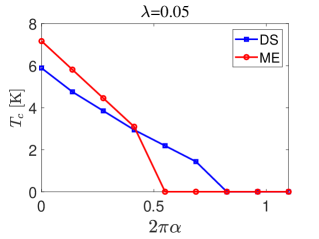
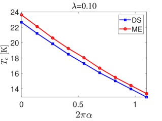
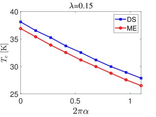
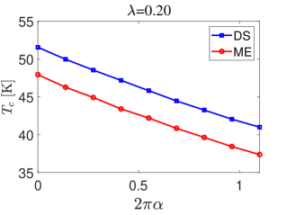
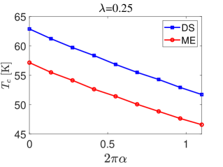
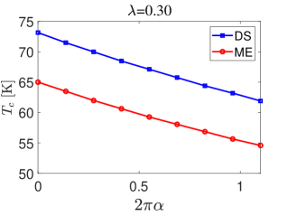
Figure 1: Comparison between results of $T_{c}$ obtained by solving ME and DS equations with six different values of $\lambda$.

After making re-scaling transformations, the electron dispersion $\xi_{\mathbf{p}}=\frac{\mathbf{p}^{2}}{2m_{e}}-\mu_{\mathrm{F}}$ is turned into $\mathbf{p}^{2}-1$, which is dimensionless. The resulting integral equations of $A_{1}$, $A_{2}$, and $\Delta$ do not explicitly depend on neither $p_{\mathrm{F}}$ nor $m_{e}$. Thus, it is not necessary to separately specify the values of $p_{\mathrm{F}}$ and $m_{e}$, since the final results of critical temperature only exhibit a dependence on $E_{\mathrm{F}}=\frac{p_{\mathrm{F}}^{2}}{2m_{e}}$. From the numerical solutions of DS and ME equations, we could obtain an effective dimensionless transition temperature, denoted by $T_{c}^{\prime}$, that is equal to $T_{c}/E_{\mathrm{F}}$. The Fermi energy $E_{\mathrm{F}}=65\mathrm{~{}meV}$ amounts to approximately $\sim 755\mathrm{~{}K}$. Then the actual transition temperature $T_{c}$ can be readily obtained from $T_{c}^{\prime}$ through the relation $T_{c}\sim T_{c}^{\prime}\times(755\mathrm{~{}K})$.

It should be emphasized that the free phonon propagator $D_{0}(q)$ is used in both the DS-level and ME-level calculations. Thus we are allowed to determine the influence of EPI vertex corrections by comparing the values of $T_{c}$ obtained under these two approximations. The pairing gap $\Delta$ is supposed to have an isotropic $s$-wave symmetry Johnston-NJP2016 . To make our analysis more generic, we consider six different values of the strength parameter $\lambda$, including $\lambda=0.05$, $\lambda=0.10$, $\lambda=0.15$, $\lambda=0.20$, $\lambda=0.25$, and $\lambda=0.30$. The numerical results of $T_{c}$ are presented in Fig. 1, where the red and blue curves correspond to the ME and DS results, respectively.

We first consider the simplest case in which the Coulomb interaction is absent. In a previous work Liu21 , it was found that including EPI vertex corrections tends to promote $T_{c}$ evaluated at the ME-level (bare vertex). This conclusion was reached based on the assumption that the electrons always strictly reside on the Fermi surface such that $\xi_{\mathbf{p}}=\xi_{\mathbf{p}_{F}}=0$ Liu21 . Here we re-solve Eqs. (68-70) without making this assumption. From the numerical results presented in Fig. 1, we observe that the impact of EPI vertex corrections on $T_{c}$ is strongly dependent of the value of EPI strength parameter $\lambda$. Specifically, we find that vertex corrections slightly reduce $T_{c}$ for $\lambda=0.10$, but considerably enhance $T_{c}$ for $\lambda=0.15$, $\lambda=0.20$, $\lambda=0.25$, and $\lambda=0.30$. The enhancement of $T_{c}$ due to vertex corrections becomes more significant as $\lambda$ further increases. The case of $\lambda=0.05$ appears to be peculiar: the vertex corrections play different roles as the effective strength of Coulomb interaction is changed.

The effect of the Coulomb interaction on $T_{c}$ can be readily investigated by varying the tuning parameter $\varepsilon$. As clearly shown by Fig. 1, $T_{c}$ drops monotonously as $\varepsilon$ decreases. Such a behavior is certainly in accordance with expectation, since the Coulomb repulsion weakens the effective attraction between electrons. In the case of $\lambda=0.05$, $T_{c}$ is slightly reduced by vertex corrections for weak Coulomb repulsion but is enhanced by vertex corrections when the Coulomb repulsion becomes strong enough. Superconductivity can be completely suppressed, with $T_{c}\rightarrow 0$, once the effective strength of Coulomb repulsion exceeds certain threshold. For larger values of $\lambda$, the Coulomb repulsion has an analogous impact on $T_{c}$. However, superconductivity could be entirely suppressed only when the repulsion becomes unrealistically strong.

For any realistic material, $\varepsilon$ takes a specific value, so does $T_{c}$. $T_{c}$ is completely determined once all the model parameters are fixed. In a way, our work provides a first-principle study of the superconducting transition, although the role of Anderson mechanism remains to be ascertained.

V Summary and Discussion

In summary, we have performed a non-perturbative study of the interplay of EPI and Coulomb repulsion by using the DS equation approach. We have shown that the DS equation of the full electron propagator $G(p)$ is self-closed provided that all the higher order corrections to EPI and Coulomb interaction are incorporated via a number of exact identities. This self-closed DS equation can be applied to study the superconducting transition beyond the ME approximation of EPI and the pseudopotential approximation of Coulomb repulsion. We have employed this approach to evaluate the pair-braking temperature $T_{c}$ for the interfacial superconductivity in 1UC FeSe/SrTiO₃ system and found that the value of $T_{c}$ could be significantly miscalculated if the vertex corrections and the momentum-dependence of relevant quantities are not taken into account in a reliable way.

The calculations of this work ignored several effects that might change the value of $T_{c}$ and thus need to be improved in the future. First of all, the simple one-band model studied by us should be replaced with a realistic multi-band model that embodies the actual electronic structure Opp-PRB2018 . The phonon self-coupling terms Johnstoncp are entirely neglected in our calculations. Including such self-coupling terms invalidates the two identities given by Eq. (50) and Eq. (52). As a consequence, the DS equation of the electron propagator $G(p)$ can no longer be made self-closed (see Ref. Liu21 and Ref. Pan21 for more details). Moreover, we did not consider the quantum geometry effects Yanase21 , which could enhance $T_{c}$ to certain extend. In this sense, our results of $T_{c}$ cannot be directly compared to the experimental values. The main achievement of our present work is a methodological advance in the non-perturbative study of the superconducting transition driven by the interplay of EPI and Coulomb repulsion.

Supplementary Material

I A Brief Introduction

We shall use the functional integral formalism of quantum field theory to derive the two Ward-Takahashi identities (WTIs) that we need to determine the self-closed integral equation of the electron propagator $G(p)$. The basic procedure of the derivation has been previously outlined in Ref. Liu2021Supp . To make our present paper self-contained and easier to understand, here we provide more calculational details.

The partition function of the model describing EPI and Coulomb interaction has the form

$$Z[J,K,\eta,\eta^{{\dagger}}]=\int D\phi DAD\psi^{{\dagger}}D\psi e^{i\int dx\mathcal{L}_{T}[\phi,A,\psi^{{\dagger}},\psi]},$$ (76)

where $\int dx\equiv\int d^{3}x=\int dtd^{2}\mathbf{x}$ and the total Lagrangian density is $\mathcal{L}_{T}=\mathcal{L}+J\phi+KA+\psi^{{\dagger}}\eta+\eta^{{\dagger}}\psi$ with $J$, $K$, $\eta$, and $\eta^{{\dagger}}$ being external sources. $\phi$ is the phonon field and $A$ is an auxiliary boson field introduced to describe the Coulomb interaction. In order to study superconducting pairing, it is convenient to adopt a two-component Nambu spinor $\psi$ to describe the electrons. The concrete form of $\mathcal{L}$ will be given later. It will become clear that the symmetry-induced WTI has the same form irrespective of whether the Coulomb interaction is included in the Lagrangian density.

For any given $\mathcal{L}_{T}$, the corresponding $Z$ can be applied to generate various important correlation functions PeskinbookSupp ; ItzyksonSupp . We are mainly interested in connected correlation functions. For this purpose, we also need to use another generating functional $W$, defined via $Z$ as follows

$$W[J,K,\eta,\eta^{{\dagger}}]=-i\ln Z[J,K,\eta,\eta^{{\dagger}}].$$ (77)

All the correlation functions to be studied below are connected. The external resources are taken to vanish ($J\rightarrow 0$, $K\rightarrow 0$,$\eta\rightarrow 0$, $\eta^{{\dagger}}\rightarrow 0$ ) after functional derivatives are done.

II Review of the work of Engelsberg and Schrieffer

In a seminal paper, Nambu Nambu60Supp made a very concise discussion of the symmetries associated with charge conservation and spin conservation in a pure EPI system and also briefly analyzed the corresponding WTIs. Later, Engelsberg and Schrieffer Schrieffer1963Supp provided a more elaborate field-theoretic analysis of the pure EPI system and, especially, derived a generic form of the charge-conservation related WTI in the normal state. Following the scenario proposed by Nambu Nambu60Supp , they argued Schrieffer1963Supp that the integral equation of EPI vertex function obtained under the ladder approximation is gauge-invariant if the vertex function is connected to the electron propagator via the WTI when the electron momentum vanishes. Their results are not satisfied for three reasons. Firstly, the ladder approximation employed in their analysis is not justified when the EPI is not weak. Secondly, their WTI in its original form cannot be used to solve the integral equation of electron propagator and thus is of little practical value. Thirdly, their analysis is restricted to the normal state and should be properly generated to treat Cooper pairing instability.

Before presenting our own work, it is helpful to first show how to derive the WTI associated with charge conservation based on the model investigated by Engelsberg and Schrieffer Schrieffer1963Supp . Their analysis were carried out by studying the Heisenberg equations of motion for the electron and phonon field operators. Our derivation will be performed within the framework of functional integral, following the general strategy demonstrated in Chapter 9 of Ref. PeskinbookSupp .

Engelsberg and Schrieffer Schrieffer1963Supp did not consider the possibility of Cooper pairing and used ordinary spinor $\Psi$, rather than Nambu spinor, to describe the electrons. The Lagrangian density defined in terms of $\Psi$ in real space is given by

$$\mathcal{\mathcal{L}}=\Psi^{{\dagger}}(x)\left(i\partial_{x_{0}}-\xi_{\nabla}\right)\Psi(x)+\frac{1}{2}A(x)\mathbb{F}(x)A(x)+\frac{1}{2}\phi^{\dagger}(x)\mathbb{D}(x)\phi(x)-A(x)\Psi^{{\dagger}}(x)\Psi(x)-g\phi(x){\Psi}^{{\dagger}}(x)\Psi(x).$$ (78)

Here, the time-space coordinate is $x\equiv(x_{0},x_{1},x_{2})$. $\partial_{x_{0}}$ represents the partial derivative $\frac{\partial}{\partial x_{0}}$ and $\xi_{\nabla}=\frac{-\mathbf{\nabla}^{2}}{2m_{e}}-\mu_{\mathrm{F}}$ with $\mathbf{\nabla}=\left(\frac{\partial}{\partial x_{1}},\frac{\partial}{\partial x_{2}}\right)$. The equations of the free motion of phonons and auxiliary scalar are $\mathbb{D}(x)\phi(x)=0$ and $\mathbb{F}(x)A(x)=0$ respectively. The EPI coupling parameter $g$ could be a constant or a function of $x$, which does not affect the final WTI. Notice that the Coulomb interaction is not included in this Lagrangian density.

Now make the following change to the spinor field $\Psi$:

$$\Psi\rightarrow{\tilde{\Psi}}=e^{i\chi(x)}\Psi.$$ (79)

Here, $\chi(x)$ is supposed to be an arbitrary infinitesimal function of $x$. The partition function $Z$ should remain the same if $\Psi$ is replaced with $\tilde{\Psi}$, namely

$$Z[J,K,\eta,\eta^{{\dagger}}]=\int D\phi DAD{\tilde{\Psi}}^{{\dagger}}D{\tilde{\Psi}}e^{i\int dx\mathcal{L}_{T}[\phi,A,{\tilde{\Psi}}^{{\dagger}},{\tilde{\Psi}}]}.$$ (80)

Usually EPI in normal metals does not lead to any quantum anomaly PeskinbookSupp , thus the functional integration measure is invariant under the above transformation, i.e., $D\Psi^{{\dagger}}D\Psi=D{\tilde{\Psi}}^{{\dagger}}D{\tilde{\Psi}}$. Then we find that

$$\int D\phi DAD{\tilde{\Psi}}^{{\dagger}}D{\tilde{\Psi}}\left[e^{i\int dx\mathcal{L}_{T}[\phi,A,{\tilde{\Psi}}^{{\dagger}},{\tilde{\Psi}}]}-e^{i\int dx\mathcal{L}_{T}[\phi,A,\Psi^{{\dagger}},\Psi]}\right]=0.$$ (81)

Since $\chi(x)$ is infinitesimal, this equation implies that

$$\int d^{3}xD\phi DA\int D{\tilde{\Psi}}^{{\dagger}}D{\tilde{\Psi}}~{}\left[\frac{\delta}{\delta\Psi(x)}e^{i\int dx\mathcal{L}_{T}}(i\chi(x)\Psi(x))+(i\chi(x)\Psi^{{\dagger}}(x))\frac{\delta}{\delta\Psi^{{\dagger}}(x)}e^{i\int dx\mathcal{L}_{T}}\right]=0.$$ (82)

It is easy to verify that

$$\frac{\delta}{\delta\Psi(x)}e^{i\int dx\mathcal{L}_{T}} = ie^{i\int dx\mathcal{L}_{T}}\left[(i\partial_{x_{0}}+\xi_{\nabla})\Psi^{{\dagger}}(x)+A(x)\Psi^{{\dagger}}(x)+g\phi(x)\Psi^{{\dagger}}(x)-\eta^{{\dagger}}(x)\right],$$ (83)

$$\frac{\delta}{\delta\Psi^{{\dagger}}(x)}e^{i\int dx\mathcal{L}_{T}} = ie^{i\int dx\mathcal{L}_{T}}\left[\left(i\partial_{x_{0}}-\xi_{\nabla}\right)\Psi(x)-A(x)\Psi(x)-g\phi(x)\Psi(x)+\eta(x)\right].$$ (84)

Substituting Eq. (83) and Eq. (84) into Eq. (82) leads to

$$0 = \Big{\langle}\int d^{3}x~{}\chi(x)\Big{[}\left((i\partial_{x_{0}}+\xi_{-\nabla})\Psi^{{\dagger}}(x)\right)\Psi(x)+g\phi(x)\Psi^{{\dagger}}(x)\Psi(x)+A(x)\Psi^{{\dagger}}(x)\Psi(x)-\eta^{{\dagger}}(x)\Psi(x)$$ (85)

$$+\Psi^{{\dagger}}(x)(i\partial_{x_{0}}-\xi_{\nabla})\Psi(x)-g\phi(x)\Psi^{{\dagger}}(x)\Psi(x)-A(x)\Psi^{{\dagger}}(x)\Psi(x)+\Psi^{{\dagger}}(x)\eta(x)\Big{]}\Big{\rangle}$$

$$= \Big{\langle}\int d^{3}x~{}\chi(x)\Big{[}i\partial_{x_{0}}\left(\Psi^{{\dagger}}(x)\Psi(x)\right)+\left(\xi_{-\nabla}\Psi^{{\dagger}}(x)\right)\Psi(x)-\Psi^{{\dagger}}(x)\left(\xi_{\nabla}\Psi(x)\right)+\Psi^{{\dagger}}(x)\eta(x)-\eta^{{\dagger}}(x)\Psi(x)\Big{]}\Big{\rangle}.$$

From the above derivations, one could find that Eq. (85) is always correct no matter whether the model contains only EPI, only Coulomb interaction, or both of them. In addition, notice that Eq. (85) holds for any continuously differentiable function $\xi_{\nabla}$. In the simplest case, the dispersion is $\xi_{\nabla}=\frac{-\mathbf{\nabla}^{2}}{2m_{e}}-\mu_{\mathrm{F}}$. If we consider a tight-binding model, then the dispersion may be of the form Johnston-NJP2016Supp $\xi_{\nabla}\equiv\xi({-i\partial_{1},-i\partial_{2}})=-t[\cos(-ia\partial_{1})+\cos(-ia\partial_{2})]-\mu_{\mathrm{F}}$, where $a$ is lattice constant. In both cases, $\xi_{-\nabla}=\xi_{\nabla}$. Since $\chi(x)$ is an arbitrary function, the following equation should be obeyed

$$\big{\langle}\big{[}i\partial_{x_{0}}\left(\Psi^{{\dagger}}(x)\Psi(x)\right)+\left(\xi_{\nabla}\Psi^{{\dagger}}(x)\right)\Psi(x)-\Psi^{{\dagger}}(x)\left(\xi_{\nabla}\Psi(x)\right)\big{]}\big{\rangle} = \langle\eta^{{\dagger}}(x)\Psi(x)\rangle-\langle\Psi^{{\dagger}}(x)\eta(x)\rangle.$$ (86)

To simplify notations and also to make a direct comparison to the work of Ref. Schrieffer1963Supp , in the following we shall take the simplest dispersion $\xi_{\nabla}=\frac{-\mathbf{\nabla}^{2}}{2m_{e}}-\mu_{\mathrm{F}}$ as an example to explain how the WTI is obtained. The generic expression of WTI has the same form if other choices of $\xi_{\nabla}$ are made. The left-hand side of Eq. (86) can be identified as the vacuum expectation value of the divergence of the composite current operator $j_{\mu}(x)\equiv\left(j_{0}(x),\mathbf{j}(x)\right)$, where

$$j_{0}(x) = \Psi^{{\dagger}}(x)\Psi(x),$$ (87)

$$\mathbf{j}(x) = \frac{1}{2m_{e}}\big{[}\left(i\mathbf{\nabla}\Psi^{{\dagger}}(x)\right)\Psi(x)-\Psi^{{\dagger}}(x)\left(i\mathbf{\nabla}\Psi(x)\right)\big{]}.$$ (88)

This identification can be readily confirmed since

$$\langle i\partial_{\mu}j_{\mu}(x)\rangle = \langle i\partial_{x_{0}}j_{0}(x)\rangle+\langle i\mathbf{\nabla}\cdot\mathbf{j}(x)\rangle$$ (89)

$$= \big{\langle}i\partial_{x_{0}}\left(\Psi^{{\dagger}}(x)\Psi(x)\right)\big{\rangle}+\frac{1}{2m_{e}}\big{\langle}i\mathbf{\nabla}\cdot\left[\left(i\mathbf{\nabla}\Psi^{{\dagger}}(x)\right)\Psi(x)-\Psi^{{\dagger}}(x)\left(i\mathbf{\nabla}\Psi(x)\right)\right]\big{\rangle}$$

$$= \big{\langle}i\partial_{x_{0}}\left(\Psi^{{\dagger}}(x)\Psi(x)\right)\big{\rangle}+\big{\langle}\left(\xi_{\nabla}\Psi^{{\dagger}}(x)\right)\Psi(x)-\Psi^{{\dagger}}(x)\left(\xi_{\nabla}\Psi(x)\right)\big{\rangle}.$$

Now the identity given by Eq. (86) can be re-written as

$$\langle i\partial_{x_{0}}j_{0}(x)+i\mathbf{\nabla}\cdot\mathbf{j}(x)\rangle=\langle\eta^{{\dagger}}(x)\Psi(x)\rangle-\langle\Psi^{{\dagger}}(x)\eta(x)\rangle.$$ (90)

If all the external resources are eliminated by taking the limit of $\eta^{{\dagger}}=\eta=0$, this identity re-produces the famous Noether theorem, i.e.,

$$\langle i\partial_{x_{0}}j_{0}(x)+i\mathbf{\nabla}\cdot\mathbf{j}(x)\rangle=0.$$ (91)

Nevertheless, it is more advantageous to keep all the external sources at the present stage. Actually, one could obtain very important results if one performs functional derivatives $\frac{\delta}{\delta\eta(z)}$ and $\frac{\delta}{\delta\eta^{{\dagger}}(y)}$ to both sides of Eq. (90) in order before taking external sources to zero. This manipulation drives the right-hand side of Eq. (90) to become

$$\frac{\delta}{\delta\eta^{{\dagger}}(y)}\frac{\delta}{\delta\eta(z)}\left[\langle\eta^{{\dagger}}(x)\Psi(x)\rangle-\langle\Psi^{{\dagger}}(x)\eta(x)\rangle\right] = \frac{\delta}{\delta\eta^{{\dagger}}(y)}\frac{\delta}{\delta\eta(z)}\left[\eta^{\dagger}(x)\frac{\delta W}{\delta\eta^{\dagger}(x)}+\frac{\delta W}{\delta\eta(x)}\eta(x)\right]$$ (92)

$$= -\delta(y-x)\frac{\delta W}{\delta\eta(z)\delta\eta^{\dagger}(x)}-\frac{\delta W}{\delta\eta^{{\dagger}}(y)\delta\eta(x)}\delta(x-z),$$

which can be readily identified as

$$\delta(y-x)G(x-z)-G(y-x)\delta(x-z).$$ (93)

In the above derivation, we have used the following identities:

$$\frac{\delta W}{\delta\eta(z)}\Big{|}_{\eta,\eta^{{\dagger}},J=0}=-\langle\Psi^{\dagger}(z)\rangle,\quad\frac{\delta W}{\delta\eta^{\dagger}(y)}\Big{|}_{\eta,\eta^{{\dagger}},J=0}=\langle\Psi(y)\rangle,$$

$$\frac{\delta^{2}W}{\delta\eta^{\dagger}(y)\delta\eta(z)}\Big{|}_{\eta,\eta^{{\dagger}},J=0}=G(y-z).$$ (94)

The same manipulation turns the right-hand side of Eq. (90) into

$$\frac{\delta}{\delta\eta^{{\dagger}}(y)}\frac{\delta}{\delta\eta(z)}\langle i\partial_{x_{0}}j_{0}(x)+i\mathbf{\nabla}\cdot\mathbf{j}(x)\rangle$$ (95)

$$= \langle i\partial_{x_{0}}j_{0}(x)\Psi(y)\Psi^{{\dagger}}(z)\rangle+\langle i\mathbf{\nabla}\cdot\mathbf{j}(x)\Psi(y)\Psi^{{\dagger}}(z)\rangle$$

$$= i\partial_{x_{0}}\big{\langle}\Psi^{{\dagger}}(x)\Psi(x)\Psi(y)\Psi^{{\dagger}}(z)\big{\rangle}+\frac{1}{2m_{e}}i\mathbf{\nabla}\cdot\big{\langle}\big{[}\left(i\mathbf{\nabla}\Psi^{{\dagger}}(x)\right)\Psi(x)-\Psi^{{\dagger}}(x)\left(i\mathbf{\nabla}\Psi(x)\right)\big{]}\Psi(y)\Psi^{{\dagger}}(z)\big{\rangle}.$$

Here, notice an important feature that the derivatives $\partial_{x_{0}}$ and $\mathbf{\nabla}$ can be freely moved out of the angle-bracket $\langle\cdots\rangle$ when the mean value is defined within the framework of function integral PeskinbookSupp .

Now define a scalar function ${\tilde{\Gamma}}_{0}$ and a vector function ${\tilde{\mathbf{\Gamma}}}=({\tilde{\Gamma}}_{1},{\tilde{\Gamma}}_{2})$ as follows

$$\big{\langle}\Psi^{{\dagger}}(x)\Psi(x)\Psi(y)\Psi^{{\dagger}}(z)\big{\rangle}=-\int d\zeta d\zeta^{\prime}G(y-\zeta){\tilde{\Gamma}}_{0}(\zeta-x,x-\zeta^{\prime})G(\zeta^{\prime}-z),$$ (96)

$$\frac{1}{2m_{e}}\big{\langle}\big{[}\left(i\mathbf{\nabla}\Psi^{{\dagger}}(x)\right)\Psi(x)-\Psi^{{\dagger}}(x)\left(i\mathbf{\nabla}\Psi(x)\right)\big{]}\Psi(y)\Psi^{{\dagger}}(z)\big{\rangle}=-\int d\zeta d\zeta^{\prime}G(y-\zeta){\tilde{\mathbf{\Gamma}}}(\zeta-x,x-\zeta^{\prime})G(\zeta^{\prime}-z),$$ (97)

Functions ${\tilde{\Gamma}}_{0}$ and ${\tilde{\mathbf{\Gamma}}}$ are called current vertex functions Liu2021Supp because they are defined in terms of the time-component $j_{0}(x)$ and the spatial component $\mathbf{j}(x)$ of the composite current operator $j_{\mu}(x)$, respectively. Then Eq. (95) is expressed in terms of ${\tilde{\Gamma}}_{0}$ and ${\tilde{\mathbf{\Gamma}}}$ as

$$-\int d\zeta d\zeta^{\prime}G(y-\zeta)i\partial_{x_{0}}{\tilde{\Gamma}}_{0}(\zeta-x,x-\zeta^{\prime})G(\zeta^{\prime}-z)-\int d\zeta d\zeta^{\prime}G(y-\zeta)i\mathbf{\nabla}\cdot{\tilde{\mathbf{\Gamma}}}(\zeta-x,x-\zeta^{\prime})G(\zeta^{\prime}-z),$$ (98)

where

$$i\partial_{x_{0}}{\tilde{\Gamma}}_{0}(\zeta-x,x-\zeta^{\prime}) \equiv i\frac{\partial}{\partial x_{0}}{\tilde{\Gamma}}_{0}(\zeta-x,x-\zeta^{\prime}),$$ (99)

$$i\mathbf{\nabla}\cdot{\tilde{\Gamma}}_{0}(\zeta-x,x-\zeta^{\prime}) \equiv i\frac{\partial}{\partial x_{1}}{\tilde{\Gamma}}_{1}(\zeta-x,x-\zeta^{\prime})+i\frac{\partial}{\partial x_{2}}{\tilde{\Gamma}}_{2}(\zeta-x,x-\zeta^{\prime}).$$ (100)

The two expressions given by Eq. (93) and Eq. (98) are equal since they both stem from Eq. (90), namely

$$-\int d\zeta d\zeta^{\prime}G(y-\zeta)\big{[}i\partial_{x_{0}}{\tilde{\Gamma}}_{0}(\zeta-x,x-\zeta^{\prime})+i\mathbf{\nabla}\cdot{\tilde{\mathbf{\Gamma}}}(\zeta-x,x-\zeta^{\prime})\big{]}G(\zeta^{\prime}-z)$$ (101)

$$= \delta(y-x)G(x-z)-G(y-x)\delta(x-z).$$

This is actually the real-space WTI. Its expression can be made less awkward by performing Fourier transformations. The Fourier transformation of the right-hand side of Eq. (101) is very simple and the result is

$$\delta(y-x)G(x-z)-G(y-x)\delta(x-z)=\int\frac{d^{3}p}{(2\pi)^{3}}\frac{d^{3}q}{(2\pi)^{3}}\left[G(p)-G(p+q)\right]e^{-i(p+q)(y-x)-ip(x-z)}.$$ (102)

The Fourier transformation of the left-hand side is a little more complicated, and can be carried out step by step. Let us take $\partial_{x_{0}}\langle\Psi^{{\dagger}}(x)\Psi(x)\Psi(y)\Psi^{{\dagger}}(z)\rangle$ as an example and show how the transformation is implemented below:

$$i\partial_{x_{0}}\langle\Psi^{{\dagger}}(x)\Psi(x)\Psi(y)\Psi^{{\dagger}}(z)\rangle$$ (103)

$$= -\int d\zeta d\zeta^{\prime}G(y-\zeta)i\partial_{x_{0}}{\tilde{\Gamma}}_{0}(\zeta-x,x-\zeta^{\prime})G(\zeta^{\prime}-z)$$

$$= -i\partial_{x_{0}}\int d\zeta d\zeta^{\prime}\int\frac{d^{3}p_{1}}{(2\pi)^{3}}G(p_{1})e^{-ip_{1}(y-\zeta)}\int\frac{d^{3}q}{(2\pi)^{3}}\frac{d^{3}p}{(2\pi)^{3}}e^{-i(p+q)(\zeta-x)}{\tilde{\Gamma}}_{0}(q,p)e^{-ip(x-\zeta^{\prime})}\int\frac{d^{3}p_{2}}{(2\pi)^{3}}G(p_{2})e^{-ip_{2}(\zeta^{\prime}-z)}$$

$$= -i\partial_{x_{0}}\int\frac{d^{3}p}{(2\pi)^{3}}\frac{d^{3}q}{(2\pi)^{3}}\left[\int\frac{d^{3}p_{1}}{(2\pi)^{3}}\frac{d^{3}p_{2}}{(2\pi)^{3}}d\zeta d\zeta^{\prime}e^{i\left(p_{1}-(p+q)\right)\zeta}e^{i(p-p_{2})\zeta^{\prime}}\right]G(p_{1}){\tilde{\Gamma}}_{0}(q,p)G(p_{2})e^{iqx-ip_{1}y+ip_{2}z}$$

$$= -i\partial_{x_{0}}\int\frac{d^{3}p}{(2\pi)^{3}}\frac{d^{3}q}{(2\pi)^{3}}\left[\int\frac{d^{3}p_{1}}{(2\pi)^{3}}\frac{d^{3}p_{2}}{(2\pi)^{3}}(2\pi)^{6}\delta(p_{1}-(p+q))\delta(p-p_{2})\right]G(p_{1}){\tilde{\Gamma}}_{0}(q,p)G(p_{2})e^{iqx-ip_{1}y+ip_{2}z}$$

$$= \int\frac{d^{3}p}{(2\pi)^{3}}\frac{d^{3}q}{(2\pi)^{3}}G(p+q)q_{0}{\tilde{\Gamma}}_{0}(q,p)G(p)e^{-i(p+q)(y-x)}e^{-ip(x-z)}.$$

Here, the electron propagator $G(y-\zeta)$ and the functions ${\tilde{\Gamma}}_{0}(\zeta-x,x-\zeta^{\prime})$ and ${\tilde{\mathbf{\Gamma}}}(\zeta-x,x-\zeta^{\prime})$ have been Fourier transformed according to the expressions presented in Appendix B of Ref. Schrieffer1963Supp . Following the same procedure, it is straightforward to obtain

$$\langle i\mathbf{\nabla}\cdot\mathbf{j}(x)\Psi(y)\Psi^{{\dagger}}(z)\rangle = \frac{1}{2m_{e}}i\mathbf{\nabla}\cdot\big{\langle}\big{[}\left(i\mathbf{\nabla}\Psi^{{\dagger}}(x)\right)\Psi(x)-\Psi^{{\dagger}}(x)\left(i\mathbf{\nabla}\Psi(x)\right)\big{]}\Psi(y)\Psi^{{\dagger}}(z)\big{\rangle}$$ (104)

$$= -\int d\zeta d\zeta^{\prime}G(y-\zeta)i\mathbf{\nabla}\cdot{\tilde{\mathbf{\Gamma}}}(\zeta-x,x-\zeta^{\prime})G(\zeta^{\prime}-z)$$

$$= -\int\frac{d^{3}p}{(2\pi)^{3}}\frac{d^{3}q}{(2\pi)^{3}}G(p+q)\mathbf{q}\cdot{\tilde{\mathbf{\Gamma}}}(q,p)G(p)e^{-i(p+q)(y-x)-ip(x-z)}.$$

Combining the results given by Eq. (103), Eq. (104), and Eq. (102) leads to

$$G(p+q)\left[q_{0}{\tilde{\Gamma}}_{0}(q,p)-\mathbf{q}\cdot{\tilde{\mathbf{\Gamma}}}(q,p)\right]G(p)=G(p)-G(p+q).$$ (105)

This identity can be readily changed into a more compact form

$$q_{0}{\tilde{\Gamma}}_{0}(q,p)-\mathbf{q}\cdot{\tilde{\mathbf{\Gamma}}}(q,p)=G^{-1}(p+q)-G^{-1}(p).$$ (106)

This is precisely the WTI obtained previously by Engelsberg and Schrieffer Schrieffer1963Supp . In order to determine the DS equation of electron propagator $G(p)$, it is necessary to first get the scalar function ${\tilde{\Gamma}}_{0}(q,p)$. However, it is apparently not possible to determine ${\tilde{\Gamma}}_{0}(q,p)$ by solving one single WTI, since the vector function ${\tilde{\mathbf{\Gamma}}}(q,p)$ is not known. Engelsberg and Schrieffer Schrieffer1963Supp did not try to made any effort to explore the structure of ${\tilde{\mathbf{\Gamma}}}(q,p)$. They simply assumed that $\mathbf{q}\cdot{\tilde{\mathbf{\Gamma}}}(q,p)=0$ as the limit $\mathbf{q}\rightarrow 0$ is taken and then simplified the WTI given by Eq. (106) into $q_{0}{\tilde{\Gamma}}_{0}(q,p)=G^{-1}(p+q)-G^{-1}(p)$ in this limit.

III Two coupled Ward-Takahashi identities in Nambu spinor representation

In order to investigate Cooper pairing, here we adopt two-component Nambu spinor $\psi$ to describe electrons. The Lagrangian density defined in terms of $\psi$ is given by

$$\mathcal{\mathcal{L}} = \psi^{{\dagger}}(x)\left(i\partial_{x_{0}}\sigma_{0}-\xi_{\nabla}\sigma_{3}\right)\psi(x)+\frac{1}{2}A(x)\mathbb{F}(x)A(x)+\frac{1}{2}\phi^{\dagger}(x)\mathbb{D}(x)\phi(x)-A(x)\psi^{{\dagger}}(x)\sigma_{3}\psi(x)$$ (107)

$$- g\phi(x){\psi}^{{\dagger}}(x)\sigma_{3}\psi(x).$$

The partition function $Z$ for this model is invariant under the following two different transformations:

$$\psi\rightarrow{\tilde{\psi}}=e^{i\chi(x)\sigma_{3}}\psi,$$ (108)

$$\psi\rightarrow{\tilde{\psi}}=e^{i\chi(x)\sigma_{0}}\psi.$$ (109)

These two transformations can be uniformly described as

$$\psi\rightarrow{\tilde{\psi}}=e^{i\chi(x)\sigma_{i}}\psi,$$ (110)

where $i=3,0$. The invariance of $Z$ leads to

$$\int D\phi DAD\psi^{{\dagger}}D\psi\left[e^{i\int dx\mathcal{L}_{T}[\phi,A,{\tilde{\psi}}^{{\dagger}},{\tilde{\psi}}]}-e^{i\int dx\mathcal{L}_{T}[\phi,A,\psi^{{\dagger}},\psi]}\right]=0,$$ (111)

which further leads to

$$\int d^{3}x\int D\phi DAD\psi^{{\dagger}}D\psi~{}\left[\frac{\delta}{\delta\psi(x)}e^{i\int dx\mathcal{L}_{T}}(i\sigma_{i}\chi(x)\psi(x))+(i\sigma_{i}\chi(x)\psi^{{\dagger}}(x))\frac{\delta}{\delta\psi^{{\dagger}}(x)}e^{i\int dx\mathcal{L}_{T}}\right]=0.$$ (112)

In the present case, one finds that

$$\frac{\delta}{\delta\psi(x)}e^{i\int dx\mathcal{L}_{T}} = ie^{i\int dx\mathcal{L}_{T}}\left[(i\partial_{x_{0}}\psi^{{\dagger}}(x)\sigma_{0}+\xi_{\nabla}\psi^{{\dagger}}(x)\sigma_{3})+A(x)\psi^{{\dagger}}\sigma_{3}+g\phi(x)\psi^{{\dagger}}(x)\sigma_{3}-\eta^{{\dagger}}(x)\right],$$ (113)

$$\frac{\delta}{\delta\psi^{{\dagger}}(x)}e^{i\int dx\mathcal{L}_{T}} = ie^{i\int dx\mathcal{L}_{T}}\left[\left(i\partial_{x_{0}}\sigma_{0}-\xi_{\nabla}\sigma_{3}\right)\psi(x)-A(x)\sigma_{3}\psi(x)-g\phi(x)\sigma_{3}\psi(x)+\eta(x)\right].$$ (114)

Inserting Eq. (113) and Eq. (114) into Eq. (112) gives rise to

$$\int d^{3}x\int D\psi^{{\dagger}}D\psi D\phi~{}e^{i\int dx\mathcal{L}_{T}}\chi(x)\big{[}-i\partial_{x_{0}}(\psi^{{\dagger}}(x)\sigma_{i}\psi(x))+\psi^{{\dagger}}(x)(\sigma_{i}\sigma_{3}\xi_{\nabla})\psi(x)-\xi_{\nabla}\psi^{{\dagger}}(x)\sigma_{3}\sigma_{i}\psi(x)$$

$$+g\phi(x)\psi^{{\dagger}}(x)[\sigma_{i},\sigma_{3}]\psi(x)+\eta^{{\dagger}}(x)\sigma_{i}\psi(x)-\psi^{{\dagger}}(x)\sigma_{i}\eta(x)\big{]}=0,$$ (115)

which, given that $\chi(x)$ is arbitrary, indicates the validity of the equation

$$\big{\langle}i\partial_{x_{0}}(\psi^{{\dagger}}(x)\sigma_{i}\psi(x))\big{\rangle}+\big{\langle}\xi_{\nabla}\psi^{{\dagger}}(x)\sigma_{3}\sigma_{i}\psi(x)\big{\rangle}-\big{\langle}\psi^{{\dagger}}(x)\sigma_{i}\sigma_{3}\xi_{\nabla}\psi(x)\big{\rangle}=\langle\eta^{{\dagger}}(x)\sigma_{i}\psi(x)\rangle-\langle\psi^{{\dagger}}(x)\sigma_{i}\eta(x)\rangle.$$ (116)

In the above derivation, we have used the relations $[\sigma_{0},\sigma_{3}]=[\sigma_{3},\sigma_{3}]=0$. Once again, this equation holds in the presence or absence of the Coulomb interaction.

For $\sigma_{i}=\sigma_{3}$, the transformation Eq. (108) corresponds to a conserved current $j^{c}_{\mu}(x)\equiv(j^{c}_{t}(x),\mathbf{j}^{c}(x))$, where

$$j^{c}_{t}(x) = \psi^{{\dagger}}(x)\sigma_{3}\psi(x),$$ (117)

$$\mathbf{j}^{c}(x) = \frac{1}{2m_{e}}\big{[}\left(i\mathbf{\nabla}\psi^{{\dagger}}(x)\right)\sigma_{0}\psi(x)-\psi^{{\dagger}}(x)\sigma_{0}\left(i\mathbf{\nabla}\psi(x)\right)\big{]}.$$ (118)

Here, notice that $j^{c}_{t}(x)$ and $\mathbf{j}^{c}(x)$ are defined by two different $2\times 2$ matrices when the two-component Nambu spinor is used to define the Lagrangian density. This current is conserved, namely $i\partial_{\mu}j_{\mu}^{c}=0$, in the absence of external sources, corresponding to the conservation of electric charge. The generic identity Eq. (116) becomes

$$\big{\langle}i\partial_{x_{0}}(\psi^{{\dagger}}(x)\sigma_{3}\psi(x))\big{\rangle}+\big{\langle}\xi_{\nabla}\psi^{{\dagger}}(x)\sigma_{0}\psi(x)-\psi^{{\dagger}}(x)\sigma_{0}\xi_{\nabla}\psi(x)\big{\rangle}=\langle\eta^{{\dagger}}(x)\sigma_{3}\psi(x)\rangle-\langle\psi^{{\dagger}}(x)\sigma_{3}\eta(x)\rangle.$$ (119)

It is easy to verify that the divergence of conserved current $j^{c}_{\mu}(x)$ has the form

$$\big{\langle}i\partial_{\mu}j^{c}_{\mu}(x)\big{\rangle} = \langle i\partial_{x_{0}}j^{c}_{t}(x)\rangle+\langle i\mathbf{\nabla}\cdot\mathbf{j}^{c}(x)\rangle$$ (120)

$$= \big{\langle}i\partial_{x_{0}}\left(\psi^{{\dagger}}(x)\sigma_{3}\psi(x)\right)\big{\rangle}+\frac{1}{2m_{e}}\big{\langle}i\mathbf{\nabla}\cdot\left[\left(i\mathbf{\nabla}\psi^{{\dagger}}(x)\right)\sigma_{0}\psi(x)-\psi^{{\dagger}}(x)\sigma_{0}\left(i\mathbf{\nabla}\psi(x)\right)\right]\big{\rangle}$$

$$= \big{\langle}i\partial_{x_{0}}\left(\psi^{{\dagger}}(x)\sigma_{3}\psi(x)\right)\big{\rangle}+\big{\langle}\left(\xi_{\nabla}\psi^{{\dagger}}(x)\right)\sigma_{0}\psi(x)-\psi^{{\dagger}}(x)\sigma_{0}\left(\xi_{\nabla}\psi(x)\right)\big{\rangle}.$$

This then allows us to re-express the identity (119) in terms of conserved current as follows

$$\langle i\partial_{\mu}j^{c}_{\mu}(x)\rangle=\langle\eta^{{\dagger}}(x)\sigma_{3}\psi(x)\rangle-\langle\psi^{{\dagger}}(x)\sigma_{3}\eta(x)\rangle.$$ (121)

The current operators need to treated very carefully. In the framework of local quantum field theory, the current operator $j^{c}_{\mu}(x)$ is defined as the product of two spinor operators $\psi^{{\dagger}}(x)$ and $\psi(x)$ at one single point $x$. Calculations based on such a definition often encounter short-distance singularities PeskinbookSupp . This is not surprising, since the charge density is apparently divergent at one single space-time point $x$. To avoid such singularities, it would be more suitable to first define the charge density in a very small cube and then take the volume of the cube to zero at the end of all calculations. The singularities of current operators could be regularized by employing the point-splitting technique. This technique was first proposed by Dirac DiracSupp , and later has been extensively applied to deal with various field-theoretic problems PeskinbookSupp ; SchwingerSupp ; Jackiw69Supp ; Callan70Supp ; Bardeen69Supp ; SchnablSupp ; He01Supp . In quantum gauge theories, such as QED and QCD, the manipulation of point-splitting destroys local gauge invariance, thus one needs to introduce a Wilson line to maintain the gauge invariance of correlation functions. Moreover, the Lorentz invariance may be explicitly broken. Fortunately, no such concerns exist in EPI systems.

In order to derive WTIs, we only need to split the position vector $\mathbf{x}$ into two close but separate points $\mathbf{x}$ and $\mathbf{x}^{\prime}$. The time $t$ need not be split. One might insist in splitting $t$ into $t$ and $t^{\prime}$, but the limit $t\rightarrow t^{\prime}$ can be taken at any time. For notational simplicity, we shall use the symbols $x$ and $x^{\prime}$. Then we re-write the composite current operators as follows

$$\psi^{{\dagger}}(x)\sigma_{0}\xi_{\nabla}\psi(x)-\xi_{\nabla}\psi^{{\dagger}}(x)\sigma_{0}\psi(x) \rightarrow \psi^{{\dagger}}(x)\sigma_{0}\xi_{\nabla_{x^{\prime}}}\psi(x^{\prime})-\xi_{\nabla_{x}}\psi^{{\dagger}}(x)\sigma_{0}\psi(x^{\prime})$$ (122)

$$= (\xi_{\nabla_{x^{\prime}}}-\xi_{\nabla_{x}})\left(\psi^{{\dagger}}(x)\sigma_{0}\psi(x^{\prime})\right).$$

We will perform various field-theoretic calculations by making use of this expression of current operator and take the limit $x\rightarrow x^{\prime}$ after all the calculations are completed.

The identity of Eq. (119) can be written as

$$i\partial_{x_{0}}\langle(\psi^{{\dagger}}(x)\sigma_{3}\psi(x))\rangle-\lim_{x^{\prime}\rightarrow x}(\xi_{\nabla_{x^{\prime}}}-\xi_{\nabla_{x}})\langle\psi^{{\dagger}}(x)\sigma_{0}\psi(x^{\prime})\rangle=\langle\eta^{{\dagger}}(x)\sigma_{3}\psi(x)\rangle-\langle\psi^{{\dagger}}(x)\sigma_{3}\eta(x)\rangle.$$ (123)

As the next step, we perform functional derivatives $\frac{\delta}{\delta\eta(z)}$ and $\frac{\delta}{\delta\eta^{{\dagger}}(y)}$ in order to both sides of this equation. The calculational procedure has already been demonstrated in Sec. II. Analytic calculations show that

$$i\partial_{x_{0}}\langle\psi^{{\dagger}}(x)\sigma_{3}\psi(x)\psi(y)\psi^{{\dagger}}(z)\rangle-\lim_{x^{\prime}\rightarrow x}(\xi_{\nabla_{x^{\prime}}}-\xi_{\nabla_{x}})\langle\psi^{{\dagger}}(x)\sigma_{0}\psi(x^{\prime})\psi(y)\psi^{{\dagger}}(z)\rangle$$ (124)

$$= \delta(y-x)\sigma_{3}G(x-z)-G(y-x)\sigma_{3}\delta(x-z).$$

For $\sigma_{i}=\sigma_{0}$. the transformation Eq. (109) corresponds to another conserved current $j^{s}_{\mu}(x)\equiv(j^{s}_{t}(x),\mathbf{j}^{s}(x))$, where

$$j^{s}_{t}(x) = \psi^{{\dagger}}(x)\sigma_{0}\psi(x),$$ (125)

$$\mathbf{j}^{s}(x) = \frac{1}{2m_{e}}\left[\left(i\mathbf{\nabla}\psi^{{\dagger}}(x)\right)\sigma_{3}\psi(x)-\psi^{{\dagger}}(x)\sigma_{3}\left(i\mathbf{\nabla}\psi(x)\right)\right].$$ (126)

Again, we see that $j^{s}_{t}(x)$ and $\mathbf{j}_{s}(x)$ are also defined by two different $2\times 2$ matrices. One might notice that, both $j^{c}_{t}(x)$ and $\mathbf{j}^{s}(x)$ involve $\sigma_{3}$, and both $j^{s}_{t}(x)$ and $\mathbf{j}^{c}(x)$ involve $\sigma_{0}$. The current of Eq. (126) is also conserved, namely $i\partial_{\mu}\langle j_{\mu}^{s}\rangle=0$, in the absence of external sources, corresponding to spin conservation. The generic identity Eq. (116) becomes

$$\langle i\partial_{x_{0}}(\psi^{{\dagger}}(x)\sigma_{0}\psi(x))\rangle+\langle\xi_{\nabla}\psi^{{\dagger}}(x)\sigma_{3}\psi(x)-\psi^{{\dagger}}(x)\sigma_{3}\xi_{\nabla}\psi(x)\rangle=\langle\eta^{{\dagger}}(x)\sigma_{0}\psi(x)\rangle-\langle\psi^{{\dagger}}(x)\sigma_{0}\eta(x)\rangle,$$ (127)

which can be re-written using the conserved current $j^{s}_{\mu}(x)$ as

$$\langle i\partial_{\mu}j^{s}_{\mu}(x)\rangle=\langle\eta^{{\dagger}}(x)\sigma_{0}\psi(x)\rangle-\langle\psi^{{\dagger}}(x)\sigma_{0}\eta(x)\rangle.$$ (128)

The identity of Eq. (127) can be written as

$$i\partial_{x_{0}}\langle(\psi^{{\dagger}}(x)\sigma_{0}\psi(x))\rangle-\lim_{x^{\prime}\rightarrow x}(\xi_{\nabla_{x^{\prime}}}-\xi_{\nabla_{x}})\langle\psi^{{\dagger}}(x)\sigma_{3}\psi(x^{\prime})\rangle=\langle\eta^{{\dagger}}(x)\sigma_{0}\psi(x)\rangle-\langle\psi^{{\dagger}}(x)\sigma_{0}\eta(x)\rangle.$$ (129)

Perform functional derivatives $\frac{\delta}{\delta\eta(z)}$ and $\frac{\delta}{\delta\eta^{{\dagger}}(y)}$ in order to both sides of this equation gives rise to

$$i\partial_{x_{0}}\langle\psi^{{\dagger}}(x)\sigma_{0}\psi(x)\psi(y)\psi^{{\dagger}}(z)\rangle-\lim_{x^{\prime}\rightarrow x}(\xi_{\nabla_{x^{\prime}}}-\xi_{\nabla_{x}})\langle\psi^{{\dagger}}(x)\sigma_{3}\psi(x^{\prime})\psi(y)\psi^{{\dagger}}(z)\rangle$$ (130)

$$= \delta(y-x)\sigma_{0}G(x-z)-G(y-x)\sigma_{0}\delta(x-z).$$

To handle the identities given by Eq. (124) and Eq. (130), we find it appropriate to define two current vertex functions $\Gamma_{3}$ and $\Gamma_{0}$ as follows

$$\langle\psi^{{\dagger}}(x)\sigma_{i}\psi(x)\psi(y)\psi^{{\dagger}}(z)\rangle=-\int d\zeta d\zeta^{\prime}G(y-\zeta)\Gamma_{i}(\zeta-x,x-\zeta^{\prime})G(\zeta^{\prime}-z),$$ (131)

where $\sigma_{0}$ corresponds to $\Gamma_{0}$ and $\sigma_{3}$ corresponds to $\Gamma_{3}$. If $x$ is splitted into two separate points $x$ and $x^{\prime}$, the above definition is changed into

$$\langle\psi^{{\dagger}}(x)\sigma_{i}\psi(x^{\prime})\psi(y)\psi^{{\dagger}}(z)\rangle=\int d\zeta d\zeta^{\prime}G(y-\zeta)\Gamma_{i}(\zeta-x,x^{\prime}-\zeta^{\prime})G(\zeta^{\prime}-z).$$ (132)

The term $i\partial_{x_{0}}\langle\psi^{{\dagger}}(x)\sigma_{i}\psi(x)\psi(y)\psi^{{\dagger}}(z)\rangle$ of Eq. (124) can be treated in the same way as what we have done in calculations shown in Eq. (103). It is straightforward to show that

$$i\partial_{x_{0}}\langle\psi^{{\dagger}}(x)\sigma_{i}\psi(x)\psi(y)\psi^{{\dagger}}(z)\rangle = -\int d\zeta d\zeta^{\prime}G(y-\zeta)i\frac{\partial}{\partial{x_{0}}}\Gamma_{i}(\zeta-x,x-\zeta^{\prime})G(\zeta^{\prime}-z)$$ (133)

$$= \int\frac{d^{3}p}{(2\pi)^{3}}\frac{d^{3}q}{(2\pi)^{3}}G(p+q)q_{0}\Gamma_{i}(q,p)G(p)e^{-i(p+q)(y-x)}e^{-ip(x-z)}.$$

The term $\lim_{x^{\prime}\rightarrow x}(\xi_{\nabla_{x^{\prime}}}-\xi_{\nabla_{x}})\langle\psi^{{\dagger}}(x)\sigma_{i}\psi(x^{\prime})\psi(y)\psi^{{\dagger}}(z)\rangle$ should be treated more carefully. According to Eq. (132), we carry out Fourier transformation as follows

$$\lim_{x^{\prime}\rightarrow x}(\xi_{\nabla_{x^{\prime}}}-\xi_{\nabla_{x}})\langle\psi^{{\dagger}}(x)\sigma_{i}\psi(x^{\prime})\psi(y)\psi^{{\dagger}}(z)\rangle$$ (134)

$$= -\lim_{x^{\prime}\rightarrow x}(\xi_{\nabla_{x^{\prime}}}-\xi_{\nabla_{x}})\int d\zeta d\zeta^{\prime}G(y-\zeta)\Gamma_{i}(\zeta-x,x^{\prime}-\zeta^{\prime})G(\zeta^{\prime}-z)$$

$$= -\lim_{x^{\prime}\rightarrow x}(\xi_{\nabla_{x^{\prime}}}-\xi_{\nabla_{x}})\int d\zeta d\zeta^{\prime}\int\frac{d^{3}p_{1}}{(2\pi)^{3}}G(p_{1})e^{-ip_{1}(y-\zeta)}\int\frac{d^{3}q}{(2\pi)^{3}}\frac{d^{3}p}{(2\pi)^{3}}e^{-i(p+q)(\zeta-x)}\Gamma_{i}(q,p)e^{-ip(x^{\prime}-\zeta^{\prime})}$$

$$\times\int\frac{d^{3}p_{2}}{(2\pi)^{3}}G(p_{2})e^{-ip_{2}(\zeta^{\prime}-z)}$$

$$= -\lim_{x^{\prime}\rightarrow x}(\xi_{\nabla_{x^{\prime}}}-\xi_{\nabla_{x}})\int\frac{d^{3}p}{(2\pi)^{3}}\frac{d^{3}q}{(2\pi)^{3}}\left[\int\frac{d^{3}p_{1}}{(2\pi)^{3}}\frac{d^{3}p_{2}}{(2\pi)^{3}}d\zeta d\zeta^{\prime}e^{i\left(p_{1}-(p+q)\right)\zeta}e^{i(p-p_{2})\zeta^{\prime}}\right]G(p_{1})\Gamma_{i}(q,p)G(p_{2})$$

$$\times e^{i(p+q)x-ipx^{\prime}-ip_{1}y+ip_{2}z}$$

$$= -\lim_{x^{\prime}\rightarrow x}(\xi_{\nabla_{x^{\prime}}}-\xi_{\nabla_{x}})\int\frac{d^{3}p}{(2\pi)^{3}}\frac{d^{3}q}{(2\pi)^{3}}\left[\int\frac{d^{3}p_{1}}{(2\pi)^{3}}\frac{d^{3}p_{2}}{(2\pi)^{3}}(2\pi)^{6}\delta\left(p_{1}-(p+q)\right)\delta(p-p_{2})\right]G(p_{1})\Gamma_{i}(q,p)G(p_{2})$$

$$\times e^{i(p+q)x-ipx^{\prime}-ip_{1}y+ip_{2}z}$$

$$= -\lim_{x^{\prime}\rightarrow x}(\xi_{\nabla_{x^{\prime}}}-\xi_{\nabla_{x}})\int\frac{d^{3}p}{(2\pi)^{3}}\frac{d^{3}q}{(2\pi)^{3}}G(p+q)\Gamma_{i}(q,p)G(p)e^{i(p+q)x-ipx^{\prime}-i(p+q)y+ipz}$$

$$= \int\frac{d^{3}p}{(2\pi)^{3}}\frac{d^{3}q}{(2\pi)^{3}}G(p+q)\left(\xi_{\mathbf{p}}-\xi_{\mathbf{p+q}}\right)\Gamma_{i}(q,p)G(p)e^{-i(p+q)(y-x)}e^{-ip(x-z)}.$$

The right-hand sides of Eq. (124) and Eq. (130) can be treated as follows

$$\delta(y-x)\sigma_{3}G(x-z)-G(y-x)\sigma_{3}\delta(x-z) = \int\frac{d^{3}p}{(2\pi)^{3}}\frac{d^{3}q}{(2\pi)^{3}}\left[\sigma_{3}G(p)-G(p+q)\sigma_{3}\right]e^{-i(p+q)(y-x)-ip(x-z)},$$ (135)

$$\delta(y-x)\sigma_{0}G(x-z)-G(y-x)\sigma_{3}\delta(x-z) = \int\frac{d^{3}p}{(2\pi)^{3}}\frac{d^{3}q}{(2\pi)^{3}}\left[\sigma_{0}G(p)-G(p+q)\sigma_{0}\right]e^{-i(p+q)(y-x)-ip(x-z)}.$$ (136)

Based on the results of Eqs. (133-136), we now obtain two identities

$$q_{0}G(p+q)\Gamma_{3}(q,p)G(p)-\left(\xi_{\mathbf{p+q}}-\xi_{\mathbf{p}}\right)G(p+q)\Gamma_{0}(q,p)G(p) = \sigma_{3}G(p)-G(p+q)\sigma_{3},$$ (137)

$$q_{0}G(p+q)\Gamma_{0}(q,p)G(p)-\left(\xi_{\mathbf{p+q}}-\xi_{\mathbf{p}}\right)G(p+q)\Gamma_{3}(q,p)G(p) = \sigma_{0}G(p)-G(p+q)\sigma_{0}.$$ (138)

They can be readily re-written in more compact forms

$$q_{0}\Gamma_{3}(q,p)-\left(\xi_{\mathbf{p+q}}-\xi_{\mathbf{p}}\right)\Gamma_{0}(q,p) = G^{-1}(p+q)\sigma_{3}-\sigma_{3}G^{-1}(p),$$ (139)

$$q_{0}\Gamma_{0}(q,p)-\left(\xi_{\mathbf{p+q}}-\xi_{\mathbf{p}}\right)\Gamma_{3}(q,p) = G^{-1}(p+q)\sigma_{0}-\sigma_{0}G^{-1}(p).$$ (140)

The WTIs given by Eq. (139) and Eq. (140) come from the symmetries defined by Eq. (108) and Eq. (109), respectively. These two WTIs involve two unknown current vertex functions, namely $\Gamma_{3}(q,p)$ and $\Gamma_{0}(q,p)$. After solving these two self-consistently coupled identities, we can determine $\Gamma_{3}(q,p)$ and $\Gamma_{0}(q,p)$ using $q_{0}$, $\xi_{\mathbf{p+q}}-\xi_{\mathbf{p}}$, and $G(p)$.

The above two WTIs have already been derived in Ref. Liu2021Supp in the case of pure EPI system. In the present work, the model contains an additional Coulomb interaction between electrons. Would the Coulomb interaction change such WTIs? No changes at all. This is because the partition function describing pure EPI and the one describing the interplay between EPI and Coulomb interaction preserve the same U(1) symmetries defined by Eq. (110).

IV Revisiting the WTI of Engelsberg and Schrieffer

The point-splitting technique plays a crucial role in the derivation of WTIs given by Eq. (139) and Eq. (140). What would one obtain if this technique is combined with the derivation of the WTI presented in Ref. Schrieffer1963Supp . According to the analysis of Sec. II, we know that the following identity holds

$$\frac{\delta}{\delta\eta^{{\dagger}}(y)}\frac{\delta}{\delta\eta(z)}\langle i\partial_{x_{0}}j_{0}(x)+i\mathbf{\nabla}\cdot\mathbf{j}(x)\rangle$$ (141)

$$= \langle i\partial_{x_{0}}j_{0}(x)\Psi(y)\Psi^{{\dagger}}(z)\rangle+\langle i\mathbf{\nabla}\cdot\mathbf{j}(x)\Psi(y)\Psi^{{\dagger}}(z)\rangle$$

$$= i\partial_{x_{0}}\big{\langle}\Psi^{{\dagger}}(x)\Psi(x)\Psi(y)\Psi^{{\dagger}}(z)\big{\rangle}+\big{\langle}\big{[}\left(\xi_{\nabla}\Psi^{{\dagger}}(x)\right)\Psi(x)-\Psi^{{\dagger}}(x)\left(\xi_{\nabla}\Psi(x)\right)\big{]}\Psi(y)\Psi^{{\dagger}}(z)\big{\rangle}$$

$$= \delta(y-x)G(x-z)-G(y-x)\delta(x-z).$$

Splitting $x$ into $x$ and $x^{\prime}$ allows us to make the following replacement

$$\big{\langle}\big{[}\left(\xi_{\nabla}\Psi^{{\dagger}}(x)\right)\Psi(x)-\Psi^{{\dagger}}(x)\left(\xi_{\nabla}\Psi(x)\right)\big{]}\Psi(y)\Psi^{{\dagger}}(z)\big{\rangle}\Rightarrow-\lim_{x\rightarrow x^{\prime}}(\xi_{\nabla_{x^{\prime}}}-\xi_{\nabla_{x}})\langle\Psi^{{\dagger}}(x)\Psi(x^{\prime})\Psi(y)\Psi^{{\dagger}}(z)\rangle,$$ (142)

which then leads to

$$i\partial_{x_{0}}\langle\Psi^{{\dagger}}(x)\Psi(x)\Psi(y)\Psi^{{\dagger}}(z)\rangle-\lim_{x^{\prime}\rightarrow x}(\xi_{\nabla_{x^{\prime}}}-\xi_{\nabla_{x}})\langle\Psi^{{\dagger}}(x)\Psi(x^{\prime})\Psi(y)\Psi^{{\dagger}}(z)\rangle$$ (143)

$$= \delta(y-x)G(x-z)-G(y-x)\delta(x-z).$$

It is now only necessary to define one single scalar function ${\tilde{\Gamma}}_{0}$ as

$$\langle\Psi^{{\dagger}}(x)\Psi(x)\Psi(y)\Psi^{{\dagger}}(z)\rangle=-\int d\xi d\xi^{\prime}G(y-\xi){\tilde{\Gamma}}_{0}(\xi-x,x-\xi^{\prime})G(\xi^{\prime}-z),$$ (144)

which becomes

$$\langle\Psi^{{\dagger}}(x)\Psi(x^{\prime})\Psi(y)\Psi^{{\dagger}}(z)\rangle=-\int d\xi d\xi^{\prime}G(y-\xi){\tilde{\Gamma}}_{0}(\xi-x,x^{\prime}-\xi^{\prime})G(\xi^{\prime}-z)$$ (145)

after splitting $x$ into $x$ and $x^{\prime}$. Then Eq. (144) and Eq. (145) can be substituted into Eq. (143), yielding the following identity

$$\int d\xi d\xi^{\prime}G(y-\xi)\big{[}i\partial_{x_{0}}{\tilde{\Gamma}}_{0}(\xi-x,x-\xi^{\prime})-\lim_{x^{\prime}\rightarrow x}(\xi_{\nabla_{x^{\prime}}}-\xi_{\nabla_{x}}){\tilde{\Gamma}}_{0}(\xi-x,x^{\prime}-\xi^{\prime})\big{]}G(\xi^{\prime}-z)$$ (146)

$$= G(y-x)\delta(x-z)-\delta(y-x)G(x-z).$$

Fourier transformation changes this identity into

$$q_{0}{\tilde{\Gamma}}_{0}(q,p)-\left(\xi_{\mathbf{p+q}}-\xi_{\mathbf{p}}\right){\tilde{\Gamma}}_{0}(q,p)=G^{-1}(p+q)-G^{-1}(p).$$ (147)

Making use of the electron dispersion $\xi_{\mathbf{p}}=\frac{\mathbf{p}^{2}}{2m_{e}}-\mu_{\mathrm{F}}$, one finds

$$\left(\xi_{\mathbf{p+q}}-\xi_{\mathbf{p}}\right){\tilde{\Gamma}}_{0}(q,p)=\mathbf{q}\cdot\frac{2\mathbf{p}+\mathbf{q}}{2m_{e}}{\tilde{\Gamma}}_{0}(q,p).$$ (148)

Comparing to Eq. (106), we see that the vector function ${\tilde{\mathbf{\Gamma}}}(q,p)$ studied in Ref. Schrieffer1963Supp can be connected to ${\tilde{\Gamma}}_{0}(q,p)$ via the relation

$${\tilde{\mathbf{\Gamma}}}(q,p)=\frac{2\mathbf{p}+\mathbf{q}}{2m_{e}}{\tilde{\Gamma}}_{0}(q,p).$$ (149)

Using Eq. (147), the scalar function ${\tilde{\Gamma}}_{0}(q,p)$ can be determined by the full electron propagator $G(p)$ via the relation

$${\tilde{\Gamma}}_{0}(q,p)=\frac{G^{-1}(p+q)-G^{-1}(p)}{q_{0}-\left(\xi_{\mathbf{p+q}}-\xi_{\mathbf{p}}\right)}.$$ (150)

References

• (1) J. R. Schrieffer, Theory of Superconductivity (Taylor and Francis, 1964).
• (2) D. J. Scalapino, in Superconductivity, edited by R. D. Parks (Marcel Dekker, Inc. New York, 1969).
• (3) P. B. Allen and B. Mitrović, Theory of Superconducting $T_{c}$, Solid State Physics, Vol.37 (Academic Press, Inc., 1982).
• (4) J. P. Carbotte, Properties of boson-exchange superconductors, Rev. Mod. Phys. 62, 1027 (1990).
• (5) F. Marsiglio, Eliashberg theory: A short review, Ann. Phys. 417, 168102 (2020).
• (6) A. Migdal, Interaction between electrons and lattice vibrations in a normal metal, Sov. Phys. JETP 7, 996 (1958).
• (7) G. M. Eliashberg, Interactions between electrons and lattice vibrations in a superconductor, Sov. Phys. JETP 11, 696 (1960).
• (8) V. V. Tolmachev, Logarithmic criterion for superconductivity, Dokl. Akad. Nauk SSSR 140, 563 (1961).
• (9) P. Morel and P. W. Anderson, Calculation of the superconducting state parameters with retarded electron-phonon interaction, Phys. Rev. 125, 1263 (1962).
• (10) J. F. Schooley, W. R. Hosler, and M. L. Cohen, Superconductivity in semiconducting SrTiO3, Phys. Rev. Lett. 12, 474 (1964).
• (11) M. N. Gastiasoro, J. Ruhman, and R. M. Fernandes, Anisotropic superconductivity mediated by ferroelectric fluctuations in cubic systems with spin-orbit coupling, Ann. Phys. 417, 168107 (2020).
• (12) H. Rietschel and L. J. Sham, Role of electron Coulomb interaction in superconductivity, Phys. Rev. B 28, 5100 (1983).
• (13) C. F. Richardson and N. W. Ashcroft, Effective electron-electron interactions and the theory of superconductivity, Phys. Rev. B 55, 15130 (1997).
• (14) T. Wang, X. Cai, K. Chen, B. V. Svistunov, and N. V. Prokof’ev, Origin of the Coulomb pseudopotential, Phys. Rev. B 107, L140507 (2022).
• (15) M. Simonato, M. I. Katsnelson, and M. Rösner, Revised Tolmachev-Morel-Anderson pseudopotential for layered conventional superconductors with nonlocal Coulomb interaction, Phys. Rev. B 108, 064513 (2023).
• (16) G.-Z. Liu, Z.-K. Yang, X.-Y. Pan, and J.-R. Wang, Towards exact solutions for the superconducting $T_{c}$ induced by electron-phonon interaction, Phys. Rev. B 103, 094501 (2021).
• (17) X.-Y. Pan, Z.-K. Yang, X. Li, and G.-Z. Liu, Nonperturbative Dyson-Schwinger equation approach to strongly interacting Dirac fermion systems, Phys. Rev. B 104, 085141 (2021).
• (18) Z.-K. Yang, X.-Y. Pan, and G.-Z. Liu, A non-perturbative study of the interplay between electron-phonon interaction and Coulomb interaction in undoped graphene, J. Phys.:Condens. Matter 35, 075601 (2022).
• (19) Y. Nambu, Quasi-particles and gauge invariance in the theory of superconductivity, Phys. Rev. 117, 648 (1960).
• (20) P. M. Dee, J. Coulter, K. G. Kleiner, and S. Johnston, Relative importance of nonlinear electron-phonon coupling and vertex corrections in the Holstein model, Communications Phys. 3, 145 (2020).
• (21) C. Itzykson and J.-B. Zuber, Quantum Field Theory, (McGraw-Hill Inc. 1980).
• (22) M. E. Peskin and D. V. Schroeder, An Introduction to Quantum Field Theory (CRC Press, 2018).
• (23) S. Engelsberg and J. R. Schrieffer, Coupled electron-phonon system, Phys. Rev. 131, 993 (1963).
• (24) A detailed derivation of the two WTIs used in our calculations is presented in the Supplementary Material. The Supplementary Material also contains Refs. [25-31].
• (25) P. A. M. Dirac, Discussion of the infinite distribution of electrons in the theory of the positron, Proc. Camb. Phil. Soc. 30, 150 (1934).
• (26) J. Schwinger, On gauge invariance and vacuum polarization, Phys. Rev. 82, 664 (1951).
• (27) R. Jackiw and K. Johnson, Anomalies of the axial-vector current, Phys. Rev. 182, 1459 (1969).
• (28) W. A. Bardeen, Anomalous Ward identities in spinor field theories, Phys. Rev. 184, 1848 (1969).
• (29) C. G. Callan, S. Coleman, and R. Jackiw, A new improved energy-momentum tensor, Ann. Phys. 59, 42 (1970).
• (30) J. Novotny and M. Schnabl, Point-splitting regularization of composite operators and anomalies, Fortschr. Phys. 48, 253 (2000).
• (31) H. He, F. C. Khanna, and Y. Takahashi, Transverse Ward-Takahashi identity for the fermion-boson vertex in gauge theories, Phys. Lett. B 480, 222 (2000).
• (32) A. A. Abrikosov, L. P. Gor’kov, and I. Y. Dzyaloshinskii, Quantum Field Theoretical Methods in Statistical Physics (Pergamon Press Inc., 1965).
• (33) A. Abanov and A. V. Chubukov, Anomalous scaling at the quantum critical point in itinerant antiferromagnets, Phys. Rev. Lett. 93, 255702 (2004).
• (34) M. A. Metlitski and S. Sachdev, Quantum phase transitions of metals in two spatial dimensions. I. Ising-nematic order, Phys. Rev. B 82, 075127 (2010).
• (35) P.-L. Zhao and G.-Z. Liu, Absence of emergent supersymmetry in superconducting quantum critical points in Dirac and Weyl semimetals, npj Quantum Materials 4, 37 (2019).
• (36) J. Aguilera Damia, M. Solis, and G. Torroba, How non-Fermi liquids cure their infrared divergences, Phys. Rev. B 102, 045147 (2020).
• (37) Q.-Y. Wang, Z. Li, W.-H. Zhang, Z.-C. Zhang, J.-S. Zhang, W. Li, H. Ding, Y.-B. Ou, P. Deng, K. Chang, J. Wen, C.-L. Song, K. He, J.-F. Jia, S.-H. Ji, Y.-Y. Wang, L.-L. Wang, X. Chen, X.-C. Ma, and Q.-K. Xue, Interface-induced high-temperature superconductivity in single unit-Cell FeSe films on SrTiO3, Chin. Phys. Lett. 29, 037402 (2012).
• (38) J. J. Lee, F. T. Schmitt, R. G. Moore, S. Johnston, Y.-T. Cui, W. Li, M. Yi, Z. K. Liu, M. Hashimoto, Y. Zhang, D. H. Lu, T. P. Devereaux, D.-H. Lee, and Z.-X. Shen, Interfacial mode coupling as the origin of the enhancement of $T_{c}$ in FeSe films on SrTiO3, Nature (London) 515, 245 (2014).
• (39) D.-H. Lee, What makes the $T_{c}$ of FeSe/SrTiO3 so high, Chin. Phys. 24, 117405 (2015).
• (40) L. P. Gor’kov, Peculiarities of superconductivity in the single-layer FeSe/SrTiO3 interface, Phys. Rev. B 93, 060507(R) (2016).
• (41) Z.-X. Li, F. Wang, D.-H. Lee, and H. Yao, What makes the $T_{c}$ of monolayer FeSe on SrTiO3 so high: a sign-problem-free quantum Monte Carlo study, Sci. Bull. 61, 925 (2016).
• (42) Y.-Y. Xiang, F. Wang, D. Wang, Q.-H. Wang, and D.-H. Lee, High-temperature superconductivity at the FeSe/SrTiO3 interface, Phys. Rev.B 86, 134508 (2012).
• (43) B. Li, Z. W. Xing, G. Q. Huang, and D. Y. Xing, Electron-phonon coupling enhanced by the FeSe/SrTiO3 interface, J. Appl. Phys. 115, 193907 (2014).
• (44) L. Rademaker, Y. Wang, T. Berlijn, and S. Johnston, Enhanced superconductivity due to forward scattering in FeSe thin films on SrTiO3 substrates, New J. Phys. 18, 022001 (2016).
• (45) M. L. Kulić and O. V. Dolgov, The electron-phonon interaction with forward scattering peak is dominant in high $T_{c}$ superconductors of FeSe films on SrTiO3 (TiO2), New J. Phys. 19, 013020(2017).
• (46) A. Aperis and P. M. Oppeneer, Multiband full-bandwidth anisotropic Eliashberg theory of interfacial electron-phonon coupling and high-$T_{c}$ superconductivity in FeSe/SrTiO3, Phys. Rev. B 97, 060501(R) (2018).
• (47) F. Schrodi, A. Aperis and P. M. Oppeneer, Induced odd-frequency superconducting state in vertex-corrected Eliashberg theory, Phys. Rev. B 104, 174518 (2021).
• (48) Y. Xie, H.-Y. Cao, Y. Zhou, S. Chen, H. Xiang, and X.-G. Gong, Oxygen vacancy induced flat phonon mode at FeSe/SrTiO3 interface, Sci. Rep. 5, 10011 (2015).
• (49) N. Nakanishi, Ward-Takahashi identities in quantum field theory with spontaneously broken symmetry, Prog. of Theore. Phys. 51, 1183 (1974).
• (50) T. Yanagisawa, Nambu-Goldstone bosons characterized by the order parameter in spontaneous symmetry breaking, J. Phys. Soc. Jap. 86, 104711 (2017).
• (51) P. W. Anderson, Plasmons, gauge invariance, and mass, Phys. Rev. 130, 439 (1963).
• (52) T. Kitamura, T. Yamashita, J. Ishizuka, A. Daido, and Y. Yanase, Superconductivity in monolayer FeSe enhanced by quantum geometry, Phys. Rev. Research 4, 023232 (2022).

References

• (1) G.-Z. Liu, Z.-K. Yang, X.-Y. Pan, and J.-R. Wang, Towards exact solutions for the superconducting Tc induced by electron-phonon interaction, Phys. Rev. B 103, 094501 (2021).
• (2) M. E. Peskin and D. V. Schroeder, An Introduction to Quantum Field Theory (CRC Press, 2018).
• (3) C. Itzykson and J.-B. Zuber, Quantum Field Theory, (McGraw-Hill Inc. 1980).
• (4) Y. Nambu, Quasi-particles and gauge invariance in the theory of superconductivity, Phys. Rev. 117, 648 (1960).
• (5) S. Engelsberg and J.R. Schrieffer, Coupled electron-phonon System, Phys. Rev. 131, 993 (1963).
• (6) P. A. M. Dirac, The quantum theory of the electron, Proc. Camb. Phil. Soc. 30, 150 (1934).
• (7) J. Schwinger, On gauge invariance and vacuum polarization, Phys. Rev. 82, 664 (1951).
• (8) R. Jackiw and K. Johnson, Anomalies of the axial-vector current, Phys. Rev. 182, 1459 (1969).
• (9) C. G. Callan, S. Coleman, and R. Jackiw, A new improved energy-momentum tensor, Ann. Phys. 59, 42 (1970).
• (10) W. A. Bardeen, Anomalous Ward Identities in Spinor Field Theories, Phys. Rev. 184, 1848 (1969).
• (11) J. Novotny and M. Schnabl, Point-splitting regularization of composite operators and anomalies, Fortschr. Phys. 48, 253 (2000).
• (12) H. He, F. C. Khanna, and Y. Takahashi, Transverse Ward-Takahashi identity for the fermion-boson vertex in gauge theories, Phys. Lett. B 480, 222 (2000).
• (13) L. Rademaker, Y. Wang, T. Berlijn, and S. Johnston, Enhanced superconductivity due to forward scattering in FeSe thin films on SrTiO3 substrates, New J. Phys. 18, 022001 (2016).