Incentive Compatibility in the Auto-bidding World

Auto-bidding has recently become a popular feature in ad auctions. This feature enables advertisers to simply provide high-level constraints and goals to an automated agent, which optimizes their auction bids on their behalf. These auto-bidding intermediaries interact in a decentralized manner in the underlying auctions, leading to new interesting practical and theoretical questions on auction design, for example, in understanding the bidding equilibrium properties between auto-bidder intermediaries for different auctions. In this paper, we examine the effect of different auctions on the incentives of advertisers to report their constraints to the auto-bidder intermediaries. More precisely, we study whether canonical auctions such as first price auction (FPA) and second price auction (SPA) are auto-bidding incentive compatible (AIC): whether an advertiser can gain by misreporting their constraints to the autobidder.

We consider value-maximizing advertisers in two important settings: when they have a budget constraint and when they have a target cost-per-acquisition constraint. The main result of our work is that for both settings, FPA and SPA are not AIC. This contrasts with FPA being AIC when auto-bidders are constrained to bid using a (sub-optimal) uniform bidding policy. We further extend our main result and show that any (possibly randomized) auction that is truthful (in the classic profit-maximizing sense), scalar invariant and symmetric is not AIC. Finally, to complement our findings, we provide sufficient market conditions for FPA and SPA to become AIC for two advertisers. These conditions require advertisers’ valuations to be well-aligned. This suggests that when the competition is intense for all queries, advertisers have less incentive to misreport their constraints.

From a methodological standpoint, we develop a novel continuous model of queries. This model provides tractability to study equilibrium with auto-bidders, which contrasts with the standard discrete query model, which is known to be hard. Through the analysis of this model, we uncover a surprising result: in auto-bidding with two advertisers, FPA and SPA are auction equivalent.

1 Introduction

Auto-bidding has become a popular tool in modern online ad auctions, allowing advertisers to set up automated bidding strategies to optimize their goals subject to a set of constraints. By using algorithms to adjust the bid for each query, auto-bidding offers a more efficient and effective alternative to the traditional fine-grained bidding approach, which requires manual monitoring and adjustment of the bids.

There are three main components in auto-bidding paradigm: 1) the advertisers who provide high-level constraints to the auto-bidders, 2) the auto-bidder agents who bid – in a decentralized manner – on behalf of each advertiser to maximize the advertiser’s value subject to their constraints, and 3) the query-level auctions where queries are sold (see Figure 1).

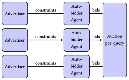
Figure 1: The Auto-bidding Process: Advertisers submit constraints and receive query allocations with specified costs as output. Inside the auto-bidding feature, each advertiser has an agent that optimizes bidding profile within each advertiser’s constraints.

Current research has made important progress in studying the interactions of the second and third components in the auto-bidding paradigm, particularly in understanding equilibrium properties (e.g., welfare and revenue) between the auto-bidders intermediaries for different auction rules (Aggarwal et al., 2019; Balseiro et al., 2021a; Deng et al., 2021a; Mehta, 2022; Liaw et al., 2022). There is also work on mechanism design for this setting in more generality, i.e., between the advertisers and the auctioneer directly abstracting out the second component (Balseiro et al., 2021c, 2022; Golrezaei et al., 2021b).

Our work, instead, examines the relation between value-maximizing advertisers, who maximize the value they obtain subject to a payment constraint, and the other two components of the auto-bidding paradigm. More precisely, we study the impact of different auction rules on the incentives of advertisers to report their constraints to the auto-bidder intermediaries. We specifically ask whether canonical auctions such as first price auction (FPA), second price auction (SPA) and general truthful auctions are auto-bidding incentive compatible (AIC) - in other words, can advertisers gain by misreporting their constraints to the auto-bidder?

We consider value-maximizing advertisers in two important settings: when they have a budget constraint and when they have a target cost-per-acquisition (tCPA) constraint. The main result of our work is that for both settings, FPA and SPA are not AIC. This contrasts with FPA being AIC when auto-bidders are constrained to bid using a (sub-optimal) uniform bidding policy. We further generalize this surprising result and show that any (possibly randomized) truthful auction having a scale invariance and symmetry property is also not AIC. We complement our result by providing sufficient market conditions for FPA and SPA to become AIC for two advertisers. These conditions require advertisers’ valuations to be well-aligned. This suggests that when the competition is intense for all queries, advertisers have less incentive to misreport their constraints.

In our model, each advertiser strategically reports a constraint (either a tCPA or a budget) to an auto-bidder agent which bids optimally on their behalf in each of the queries. Key in our model, we consider a two stage game where first advertisers submit constraints to the auto-bidders and, in the subgame, auto-bidders reach a bidding equilibrium across all query-auctions. Thus, when an advertiser deviates and reports a different constraint to its auto-bidder, the whole bidding subgame equilibrium can change. In this context, an auction rule is called auto-bidding incentive compatible (AIC) if, for all equilibria, it is optimal for the advertiser to report their constraint to the auto-bidder.

1.1 Main Results

We begin our results by presenting a stylized example in Section 2 that demonstrates how auto-bidding with SPA is not AIC (Theorem 2.1). Our example consists of a simple instance with three queries and two advertisers. This example highlights a scenario where an advertiser can benefit from lowering their reported budget or tCPA-constraint.

We then introduce a continuous query model that departs from the standard auto-bidding model by considering each query to be of infinitesimal size. This model provides tractability in solving equilibrium for general auction rules like FPA which is key to study the auto-bidding incentive compatibility properties of such auctions. Further, this continuous-query model succinctly captures real-world scenarios where the value of a single query is negligible compared to the pool of all queries that are sold.

Under the continuous-query model, we study the case where queries are sold using FPA and show that in the auto-bidding paradigm, FPA is not AIC (Section 4). We first characterize the optimal bidding strategy for each auto-bidder agent which, surprisingly, has a tractable form. We then leverage this tractable form to pin down an equilibrium for the case of two auto-bidders when both auto-bidders either face a budget or tCPA constraint. In this equilibrium, queries are divided between the two advertisers based on the ratio of their values for each advertiser. Specifically, advertiser 1 receives queries for which the ratio of its value to the other advertiser’s value is higher than a certain threshold. From this point, determining the equilibrium reduces to finding a threshold that make advertisers’ constraints tight (see Lemma 4.4 for more detail). We then show that for instances where the threshold lacks monotonicity with the auto-bidders constraints, advertisers have an incentive to misreport the constraint to the auto-bidder (Theorem 4.1). Conversely, when the thresholds are monotone advertisers report constraints truthfully. We show conditions on the advertisers’ valuations, for the two-advertisers setting, to guarantee this monotonicity (Theorem 4.10). This condition requires a strong positive correlation of the advertisers’ valuations across the queries. As a practical insight, our results suggest that for settings where the competition on all queries is intense, advertisers’ incentives to misreport is weak.

We then explore the case where, in FPA, auto-bidders are constrained to bid using a uniform bidding strategy: the bid on each query is a constant times the advertiser’s value for the query. Uniform bidding is only an optimal strategy when auctions are truthful (Aggarwal et al., 2019). Even though for FPA these strategies are suboptimal, they have gained recent attention in the literature due to their tractability Conitzer et al. (2022a, b); Chen et al. (2021); Gaitonde et al. (2022). We show that in such a scenario, FPA with uniform bidding turns out to be AIC (Theorem 4.2). However, we note that while this proves AIC in our model, the suboptimality of uniform bidding for FPA can give rise to incentives to deviate in other ways outside our model, e.g., by splitting the advertising campaigns into multiple campaigns with different constraints. These considerations are important when implementing this rule in practice.

The second part of the paper pivots to the case where auctions are truthful, that is, auctions in which it is optimal for a profit-maximizing agent to bid their value. We first study the canonical SPA and show that, in our continuous-query model, SPA and FPA are auction equivalent. That is, the allocation and payments among the set of reasonable equilibria (Theorem 5.5). As a Corollary, the results we obtain for FPA apply to SPA as well: SPA is not AIC and; and we derive sufficient conditions on advertisers’ valuations so that SPA is AIC for two advertisers. We then consider a general class of randomized truthful auctions. We show that if the allocation rule satisfies these natural conditions: (i) scaled invariant (if all bids are multiplied by the same factor then the allocation doesn’t change), and (ii) is symmetric (bidders are treated equally); then the auction rule is not AIC.

The main results of the paper are summarized in Table 1.

Per Query Auction	AIC
Second-Price Auction	Not AIC
Truthful Auctions	Not AIC
First-Price Auction	Not AIC
First-Price Auction with Uniform Bidding	AIC

Table 1: Main Results

1.2 Related Work

The study of auto-bidding in ad auctions has gained significant attention in recent years. One of the first papers to study this topic is Aggarwal et al. (2019), which presents a mathematical formulation for the auto-bidders problem given a fixed constraints reported by advertisers. They show that uniform bidding is an optimal strategy if and only if auctions are truthful (in the profit-maximizing sense). They further started an important line of work to measure, using a Price of Anarchy (PoA) approach, the welfare implications when auto-bidders are bidding in equilibrium for different auctions. Current results state that for SPA the PoA is $2$ Aggarwal et al. (2019) and also for FPA Liaw et al. (2022), and, interestingly, it can be improved if the auction uses a randomized allocation rule Mehta (2022); Liaw et al. (2022). In a similar venue, Deng et al. (2021b); Balseiro et al. (2021b) studies models where the auction has access to extra information and show how reserves and boosts can be used to improve welfare and efficiency guarantees.

A second line of work, studies how to design revenue-maximizing auctions when bidders are value-maximizing agents and may have private information about their value or their constraints (Golrezaei et al., 2021b; Balseiro et al., 2021c, b). In all these settings, the mechanism designer is not constrained to the presence of the auto-bidding intermediaries (Component 2 in Figure 1). Our study has added structure by having advertisers submit their constraints first, followed by a decentralized subgame to achieve a bidding equilibrium before allocating and determining payments. Thus, a priori their mechanism setting can achieve broader outcomes than in our auto-bidding constraint paradigm. Interestingly, for the one query case the authors show that FPA with a uniform bidding policy is optimal Balseiro et al. (2021c). Our results complement theirs and show that such mechanism is implementable in auto-bidding constraint paradigm and is AIC.

Closer to our auto-bidding paradigm, a recent line of work has started to study the incentive of advertisers when bidding via an auto-bidder intermediary. Mehta and Perlroth (2023) show that a profit-maximizing agent may benefit by reporting a target-based bidding strategy to the auto-bidder when the agent has concern that the auctioneer may change (ex-post) the auction rules. Also, in an empirical work, Li and Tang (2022) develop a new methodology to numerically approximate auto-bidding equilibrium and show numerical examples where advertisers may benefit my reporting their constraints on SPA. Our work complements their findings by showing under a theoretical framework that SPA is not AIC.

Our work also connects with the literature about auction with budgeted constraint bidders. In particular, our results are closely related to Conitzer et al. (2022a) who study FPA with uniform bidding (a.k.a. pacing bidding). They introduce the concept of the first-price auction pacing equilibrium (FPPE) for budget-constrained advertisers, which is the same as the equilibrium in our auto-bidding subgame. They show that in FPPE the revenue and welfare are monotone increasing as a function of the advertisers’ budgets. In our work, we show that in FPPE, advertisers’ values are monotone as a function of their reported budget. In addition, they differentiate between first and second-price by showing that FPPE is computable, unlike SPPE, where maximizing revenue has previously been known to be NP-hard Conitzer et al. (2022b), and that the general problem of approximating the SPPE is PPAD-complete Chen et al. (2021). In contrast, we show in the continuous model both SPA and FPA are tractable. Interestingly, this dichotomy between FPA and SPA (both with uniform bidding) is reflected in our work as well – the former is AIC, while the latter is not.

Uniform bidding has been explored in a separate body of research on repeated auctions, without the presence of auto-bidding. Balseiro and Gur (2019) investigate strategies to minimize regret in simultaneous first-price auctions with learning. Gaitonde et al. (2022) take this concept further by extending the approach to a wider range of auction settings. Furthermore, Golrezaei et al. (2021a) examines how to effectively price and bid for advertising campaigns when advertisers have both ROI and budget constraints.

2 Warm Up: Second Price Auction is not AIC!

To understand the implications of the auto-bidding model, we start with an example of auto-bidding with the second-price auction. Through this example, we will demonstrate the process of determining the equilibrium in an auto-bidding scenario and emphasize a case where the advertiser prefers to misreport their budget leading to the following theorem.

Theorem 2.1.

For the budget setting (when all advertisers are budgeted-constrained) and for the tCPA-setting (when all advertisers are tCPA-constrained), we have that SPA is not AIC. That is, there are some instances where an advertiser benefits by misreporting its constraint.

Proof.

Consider two budget-constrained advertisers and three queries $Q=\{q_{1},q_{2},q_{3}\}$, where the expected value of winning query $q$ for advertiser $a$ is denoted by $v_{a}(q)$, and it is publicly known (as in Table 2). At first, each advertiser reports their budget to the auto-bidder $B_{1}=2$, and $B_{2}=4$. Then the auto-bidder agents, one for each advertiser, submit the bidding profiles (to maximize their advertisers’ value subject to the budget constraint). The next step is a second-price auction per query, where the queries are allocated to the highest bidder.

	$q_{1}$	$q_{2}$	$q_{3}$
Advertiser 1	4	3	2
Advertiser 2	1	1.3	10

Table 2: SPA with two budget constraint advertisers is not AIC: The value of each query for each advertiser.

Finding the equilibrium bidding strategies for the auto-bidder agents is challenging, as the auto-bidder agents have to find the best-response bids with respect to the other auto-bidder agents, and each auto-bidder agent’s bidding profile changes the cost of queries for the rest of the agents. To calculate such an equilibrium between auto-bidder agents, we use the result of Aggarwal et al. (2019) to find best-response strategies. Their result states that the best response strategy in any truthful auto-bidding auction is uniform bidding. In other words, each agent optimizes over one variable, a bidding multiplier $\mu_{a}$, and then bids on query $q$ with respect to the scaled value $\mu_{a}v_{a}(q)$.

We show that with the given budgets $B_{1}=2$ and $B_{2}=4$, an equilibrium exists such that advertiser $1$ only wins $q_{1}$, and $\mu_{1}=0.5$ and $\mu_{2}=1$ result in such an equilibrium. To this end, we need to check: 1) Allocation: with bidding strategies $\mathbf{b}_{1}=(\mu_{1}v_{1}(q_{1}),\mu_{1}v_{1}(q_{2}),\mu_{1}v_{1}(q_{3}))$ and $\mathbf{b}_{2}=(\mu_{2}v_{2}(q_{1}),\mu_{2}v_{2}(q_{2}),\mu_{2}v_{2}(q_{3}))$, advertiser 1 wins $q_{1}$ and advertiser 2 wins $q_{2}$ and $q_{3}$, 2) Budget constraints are satisfied, and 3) Bidding profiles are the best response: The auto-bidder agents do not have the incentive to increase their multiplier to get more queries. These three conditions are checked as follows:

1. Allocation inequalities: For each query, the advertiser with the highest bid wins it.

   $$\frac{v_{1}(q_{1})}{v_{2}(q_{1})}\geq\frac{\mu_{2}}{\mu_{1}}=\frac{1}{0.5}\geq\frac{v_{1}(q_{2})}{v_{2}(q_{2})}\geq\frac{v_{1}(q_{3})}{v_{2}(q_{3})}.$$

2. Budget constraints: Since the auction is second-price the cost of query $q$ for advertiser 1 is $\mu_{2}v_{2}(q)$ and for advertiser 2 is $\mu_{1}v_{1}(q)$. So, we must have the following inequalities to hold so that the budget constraints are satisfied:

   $$2=B_{1}\geq\mu_{2}v_{2}(q_{1})=1\qquad\text{(Advertiser 1)},$$

   $$4=B_{2}\geq\mu_{1}(v_{1}(3)+v_{1}(q_{2}))=2.5\qquad\text{(Advertiser 2)}.$$

3. Best response: Does the advertiser’s agent have incentive to raise their multiplier to get more queries? If not, they shouldn’t afford the next cheapest query.

   $$2<\mu_{2}(v_{2}(q_{1})+v_{2}(q_{2}))=2.3\qquad\text{(Advertiser 1)},$$

   $$4<\mu_{1}(v_{1}(q_{3})+v_{1}(q_{2})+v_{1}(q_{1}))=4.5\qquad\text{(Advertiser 2)}.$$

Since all the three conditions are satisfied. Thus, this profile is an equilibrium for th auto-bidders bidding game. In this equilibrium, advertiser 1 wins $q_{1}$ and advertiser 2 wins $q_{2}$ and $q_{3}$.

Now, consider the scenario that advertiser 1 wants to strategically report their budget $B_{1}$ to the auto-bidder. Suppose the first advertiser decreases their budget. Intuitively, the budget constraint for the auto-bidder agent should be harder to satisfy, and hence the advertiser should not win more queries. But, contrary to this intuition, when advertiser $1$ reports a lower budget $B_{1}^{\prime}=1$, we show that, given the unique auto-bidding equilibrium, advertiser 1 wins $q_{1}$ and $q_{2}$ (more queries than the case where advertiser 1 reports $B_{1}=2$). Similar to above, we can check that $\mu_{1}^{\prime}=\frac{1}{2.3}$, and $\mu_{2}^{\prime}=1$ results in an equilibrium (we prove the uniqueness in Appendix A):

1. Allocation: advertiser 1 wins $q_{1}$ and $q_{2}$ since it has a higher bid on them,

   $$\frac{v_{1}(q_{1})}{v_{2}(q_{1})}\geq\frac{v_{1}(q_{2})}{v_{2}(q_{2})}\geq\frac{\mu^{\prime}_{2}}{\mu^{\prime}_{1}}=\frac{1}{2.3}\geq\frac{v_{1}(q_{3})}{v_{2}(q_{3})}.$$

2. Budget constraints:

   $$4\geq v_{1}(q_{3}),\qquad\text{and }$$

   $$1=(1/2.3)(v_{2}(q_{1})+v_{2}(q_{2})).$$

3. Best response:

   $$4<1(v_{1}(q_{3})+v_{1}(q_{2})),\qquad\text{and}$$

   $$1<(1/2.3)(v_{2}(q_{1})+v_{2}(q_{2})+v_{2}(q_{3})).$$

This surprising example leads to the first main result of the paper. In Appendix A, we will generalize the above example to the case of tCPA-constrained advertisers with the same set of queries as in Table 2. ∎

Before studying other canonical auctions, in the next section we develop a tractable model of continuous query. Under this model it turns out that the characterization of the auto-bidders bidding equilibria when the auction is not SPA is tractable. This tractability is key for studying auto-bidding incentive compatibility.

3 Model

The baseline model consists of a set of $A$ advertisers competing for $q\in Q$ single-slot queries owned by an auctioneer. We consider a continuous-query model where $Q=[0,1]$. Let $x_{a}(q)$ be the probability of winning query $q$ for advertiser $a$. Then the expected value and payment of winning query $q$ at price $p_{a}(q)$ are $x_{a}(q)v_{a}(q)dq$ and $p_{a}(q)dq$.^, Intuitively, this continuous-query model is a first-order approximation for instances where the size of each query relative to the whole set is small.

The auctioneer sells each query $q$ using a query-level auction which induces the allocation and payments $(x_{a}(q),p_{a}(q))_{a\in A}$ as a function of the bids $(b_{a})_{a\in A}$. In this paper, we focus on the First Price Auction (FPA), Second Price Auction (SPA) and more generally any Truthful Auction (see Section 5.2 for details).

Auto-bidder agent:

Advertisers do not participate directly in the auctions, rather they report high-level goal constraints to an auto-bidder agent who bids on their behalf in each of the queries. Thus, Advertiser $a$ reports a budget constraint $B_{a}$ or a target cost-per-acquisition constraint (tCPA) $T_{a}$ to the auto-bidder. Then, the auto-bidder taking as fixed other advertiser’s bid, submits bids $b_{a}(q)$ to induce $x_{a}(q),p_{a}(q)$ that solves

$$\max \int_{0}^{1}x_{a}(q)v_{a}(q)dq$$ (1)

s.t. $$\int_{0}^{1}p_{a}(q)dq\leq B_{a}+T_{a}\int_{0}^{1}x_{a}(q)v_{a}(q)dq.$$ (2)

The optimal bidding policy does not have a simple characterization for a general auction. However, when the auction is truthful (like SPA) the optimal bid take a simple form in the continuous model. (Aggarwal et al., 2019).

Remark 3.1 (Uniform Bidding).

If the per-query auction is truthful, then uniform bidding is the optimal policy for the autobidder. Thus, $b_{a}(q)=\mu\cdot v_{a}(q)$ for some $\mu>0$. We formally prove this in Claim 5.4.

Advertisers

Following the current paradigm in autobidding, we consider that advertisers are value-maximizers and can be two of types: a budget-advertiser or tCPA-advertiser. Payoffs for these advertisers are as follows.

• For a budget-advertiser with budget $B_{a}$, the payoff is

  $$u_{a}=\begin{cases}\int_{0}^{1}x_{a}(q)v_{a}(q)dq&\mbox{ if }\int_{0}^{1}p_{a}(q)dq\leq B_{a}\\ -\infty&\mbox{ if not}.\end{cases}$$

• For a tCPA-advertiser with target $T_{a}$, the payoff is

  $$u_{a}=\begin{cases}\int_{0}^{1}x_{a}(q)v_{a}(q)dq&\mbox{ if }\int_{0}^{1}p_{a}(q)dq\leq T_{a}\cdot\int_{0}^{1}x_{a}(q)v_{a}(q)dq\\ -\infty&\mbox{ if not}.\end{cases}$$

Game, Equilibrium and Auto-bidding Incentive Compatibility (AIC)

The timing of the game is as follows. First, each advertiser depending on their type submits a budget or target constraint to an auto-bidder agent. Then, each auto-bidder solves Problem 1 for the respective advertiser. Finally, the per-query auctions run and allocations and payments accrue.

We consider a complete information setting and use subgame perfect equilibrium (SPE) as solution concept. Let $V_{a}(B^{\prime}_{a};B_{a})$ the expected payoff in the subgame for a budget-advertiser with budget $B_{a}$ that reports $B^{\prime}_{a}$ to the auto-bidder (likewise we define $V_{a}(T^{\prime}_{a};T_{a})$ for the tCPA-advertiser).

Definition 3.2 (Auto-bidding Incentive Compatibility (AIC)).

An auction rule is Auto-bidding Incentive Compatible (AIC) if for every SPE we have that $V_{a}(B_{a};B_{a})\geq V_{a}(B^{\prime}_{a};B_{a})$ and $V_{a}(T_{a};T_{a})\geq V_{a}(T^{\prime}_{a};T_{a})$ for every $B_{a},B^{\prime}_{a},T_{a},T^{\prime}_{a}$.

Similar to classic notion of incentive compatibility, an auction rule satisfying AIC makes the advertisers’ decision simpler: they simply need to report their target to the auto-bidder. However, notice that the auto-bidder plays a subgame after advertiser’s reports. Thus, when Advertiser $a$ deviates and submit a different constraint, the subgame outcome may starkly change not only on the bids of Advertiser $a$ but also other advertisers bid may change as well.

4 First Price Auctions

In this section, we demonstrate that the first price auction is not auto-bidding incentive compatible.

Theorem 4.1.

Suppose that there are at least two budget-advertisers or two tCPA-advertisers, then FPA is not AIC.

Later in Section 4.2, we show a complementary result by providing sufficient conditions on advertisers’ value functions to make FPA be AIC for the case of two advertisers. We show that this sufficient condition holds in many natural settings, suggesting that in practice FPA tends to be AIC.

Then in Section 4.3, we turn our attention to FPA where autobidders are restricted to use uniform bidding across the queries. In this case, we extend to our continuous-query model the result of Conitzer et al. (2022a) and show the following result.

Theorem 4.2.

FPA restricted to uniform bidding is AIC.

4.1 Proof of Theorem 4.1

We divide the proof of Theorem 4.1 in three main steps. Step 1 characterizes the best response bidding profile for an autobidder in the subgame. As part of our analysis, we derive a close connection between first and second price auctions in the continuous-query model that simplifies the task of finding the optimal bidding for each query to finding a single multiplying variable for each advertiser.

In Step 2, we leverage the tractability of our continuous-query model and pin-down the subgame bidding equilibrium when there are either two budget-advertisers or two tCPA-advertisers in the game (Lemma 4.4). We derive an equation that characterizes the ratio of the multipliers of each advertiser as a function of the constraints submitted by the advertisers. This ratio defines the set of queries that each advertiser wins, and as we will see the value accrued by each advertiser is monotone in this ratio. So, to find a non-AIC example, one has to find scenarios where the equilibrium ratio is not a monotone function of the input constraints which leads to the next step.

To conclude, we show in Step 3 an instance where the implicit solution for the ratio is nonmonotonic, demonstrating that auto-bidding in first-price auctions is not AIC. As part of our proof, we interestingly show that AIC is harder to satisfy when advertisers face budget constraints rather than tCPA constraints (see Corollary 4.6).

Step 1: Optimal Best Response

The following claim shows that, contrary to the discrete-query model, the best response for the autobidder in a first price auction can be characterized as function of a single multiplier.

Claim 4.3.

Taking other auto-bidders as fixed, there exists a multiplier $\mu_{a}\geq 0$ such that the following bidding strategy is optimal:

$$b_{a}(q)=\begin{cases}\max_{a^{\prime}\neq a}(b_{a^{\prime}}(q))&\mu_{a}v_{a}(q)\geq\max_{a^{\prime}\neq a}(b_{a^{\prime}}(q))\\ 0&\mu_{a}v_{a}(q)\neq\max_{a^{\prime}}(b_{a^{\prime}}(q)).\end{cases}$$

The result holds whether the advertiser is budget-constrained or tCPA-constrained.

Proof.

We show that in a first-price auction, the optimal bidding strategy is to bid on queries with a value-to-price ratio above a certain threshold. To prove this, we assume that the bidding profile of all advertisers is given. Since the auction is first-price, advertiser $a$ can win each query $q$ by fixing small enough $\epsilon>0$ and paying $\max_{a^{\prime}\neq a}(b_{a^{\prime}}(q))+\epsilon$. So, let $p_{a}(q)=\max_{a^{\prime}\neq a}(b_{a^{\prime}}(q))$, be the price of query $q$. Since we have assumed that the value functions of all advertisers are integrable (i.e., there are no measure zero sets of queries with a high value), in the optimal strategy $p_{a}$ is also integrable since it is suboptimal for any advertiser to bid positive (and hence have a positive cost) on a measure zero set of queries.

First, consider a budget-constrained advertiser. The main idea is that since the prices are integrable, the advertiser’s problem is similar to a continuous knapsack problem. In a continuous knapsack problem, it is well known that the optimal strategy is to choose queries with the highest value-to-cost ratio Goodrich and Tamassia (2001). Therefore, there must exist a threshold, denoted as $\mu$, such that the optimal strategy is to bid on queries with a value-to-price ratio of at least $\mu$. So if we let $\mu_{a}=\frac{1}{\mu}$, then advertiser $a$ bids on any query with $\mu_{a}v_{a}(q)\geq p_{a}(q)$.

We prove it formally by contradiction. Assume to the contrary, that there exist non-zero measure sets $X,Y\subset Q$ such that for all $x\in X$ and $y\in Y$, the fractional value of $x$ is less than the fractional value of $y$, i.e., $\frac{v_{a}(x)}{p_{a}(q_{x})}<\frac{v_{a}(y)}{p_{a}(y)}$, and in the optimal solution advertiser $a$ gets all the queries in $X$ and no query in $Y$. However, we show that by swapping queries in $X$ with queries in $Y$ with the same price, the advertiser can still satisfy its budget constraint while increasing its value.

To prove this, fix $0<\alpha<\min(\int_{X}p_{a}(q)dq,\int_{Y}p_{a}(q)dq)$. Since the Lebesgue measure is atomless, there exists subsets $X^{\prime}\subseteq X$ and $Y^{\prime}\subseteq Y$ such that $\alpha=\int_{X^{\prime}}p_{a}(q)dq=\int_{Y^{\prime}}p_{a}(q)dq$. Since the value per cost of queries in $Y$ is higher than queries in $X$, by swapping queries of $X^{\prime}$ with $Y^{\prime}$, the value of the new sets increases, while the cost does not change. Therefore, the initial solution cannot be optimal.

A similar argument holds for tCPA-constrained advertisers. Swapping queries in $X^{\prime}$ with $Y^{\prime}$ does not change the cost and increases the upper bound of the tCPA constraint, resulting in a feasible solution with a higher value. Therefore, the optimal bidding strategy for tCPA constraint is also $b_{a}(q)$ as defined in the statement of the claim.∎

Step 2: Equilibrium Characterization

The previous step showed that the optimal bidding strategy is to bid on queries with a value-to-price ratio above a certain threshold. Thus, we need to track one variable per auto-bidder to find the subgame equilibrium.

In what follows, we focus on the case of finding the variables when there are only two advertisers in the game. This characterization of equilibrium gives an implicit equation for deriving the equilibrium bidding strategy, which makes the problem tractable in our continuous-query model..

From Claim 4.3 we observe that the ratio of bidding multipliers is key to determine the set of queries that each advertiser wins. To map the space of queries to the bidding space, we introduce the function $h(q)=\frac{v_{1}(q)}{v_{2}(q)}$. Hence, for high values of $h$, the probability that advertiser 1 wins the query increases. Also, notice that without loss of generality, we can reorder the queries on $[0,1]$ so that $h$ is non-decreasing.

In what follows, we further assume that $h$ is increasing on $[0,1]$. This implies that $h$ is invertible and also differentiable almost everywhere on $[0,1]$. With these assumptions in place, we can now state the following lemma to connect the subgame equilibrium to the ratio of advertisers’ values.

Lemma 4.4.

[Subgame Equilibrium in FPA] Given two budget-constrained auto-bidders with budget $B_{1}$ and $B_{2}$, let $\mu_{1}$ and $\mu_{2}$ be as defined in Claim 4.3 for auto-bidding with FPA. Also assume that $h(q)=\frac{v_{1}(q)}{v_{2}(q)}$ as defined above is strictly monotone. Then $\mu_{1}=\frac{B_{2}}{E[z\mathbbm{1}(z\geq r)]}$ and $\mu_{2}=\mu_{1}r$, where $r$ is the solution of the following implicit function,

$$\frac{rE[\mathbbm{1}[z\geq r)]}{E[z\mathbbm{1}(z\leq{r})]}=\frac{B_{1}}{B_{2}}.$$ (3)

Here, $E[\cdot]$ is defined as $E[P(z)]=\int_{0}^{\infty}P(z)f(z)dz,$ where $f(z)=\frac{v_{2}(h^{-1}(z))}{h^{\prime}(h^{-1}(z))}$ wherever $h^{\prime}$ is defined, and it is zero otherwise.

Also, for two tCPA auto-bidders with targets $T_{1}$ and $T_{2}$, we have $\mu_{1}=\frac{T_{1}E[\mathbbm{1}(z\leq r)]}{E[\mathbbm{1}(z\geq r)]}$ and $\mu_{2}=\mu_{1}r$, where $r$ is the answer of the following implicit function,

$$\frac{rE[\mathbbm{1}(z\geq r)]}{E[z\mathbbm{1}(z\geq{r})]}\frac{E[\mathbbm{1}(z\leq r)]}{E[z\mathbbm{1}(z\leq{r})]}=\frac{T_{1}}{T_{2}}.$$ (4)

Remark 4.5.

The function $f$ intuitively represents the expected value of the queries that advertiser 2 can win as well as the density of the queries that advertiser 1 can win. Also, the variable $r$ shows the cut-off on how the queries are divided between the two advertisers. In the proof, we will see that the advertisers’ value at equilibrium is computed with respect to $f$: Advertiser 1’s overall value is $\int_{r}^{\infty}zf(z)dz$ and advertiser 2’s overall value is $\int_{0}^{r}f(z)dz$.

Proof.

First, consider budget constraint auto-bidders. Given Claim 4.3, in equilibrium price of query $q$ is $\min(\mu_{1}v_{1}(q),\mu_{2}v_{2}(q))$. Therefore, the budget constraints become:

$$B_{1}=\int_{0}^{1}{\mu_{2}v_{2}(q)}\mathbbm{1}({\mu_{2}v_{2}(q)}\leq\mu_{1}v_{1}(q))dq,$$

$$B_{2}=\int_{0}^{1}{\mu_{1}v_{1}(q)}\mathbbm{1}({\mu_{2}v_{2}(q)}\geq\mu_{1}v_{1}(q))dq.$$

With a change of variable from $q$ to $z=h(q)$ and letting $r=\frac{\mu_{2}}{\mu_{1}}$, we have:

$$B_{1}=\int_{r}^{\infty}{\mu_{2}v_{2}(h^{-1}(z))}\frac{dh^{-1}(z)}{dz}dz$$

$$B_{2}=\int_{0}^{r}{\mu_{1}v_{1}(h^{-1}(z))}\frac{dh^{-1}(z)}{dz}dz.$$

Observe that $v_{1}(h^{-1}(z))=zv_{2}(h^{-1}(z))$, then if we let $f(z)=v_{2}(h^{-1})(h^{-1})^{\prime}=\frac{v_{2}(h^{-1}(z))}{h^{\prime}(h^{-1}(z))}$, the constraints become

$$B_{1}=\mu_{2}\int_{r}^{\infty}f(z)dz,$$ (5)

$$B_{2}=\mu_{1}\int_{0}^{r}zf(z)dz.$$ (6)

We obtain Equation (3) by diving both sides of Equation (5) by the respective both sides of Equation (6).

Now, consider two tCPA constrained auto-bidders. Similar to the budget-constrained auto-bidders, we can write

$$T_{1}\int_{0}^{1}{v_{1}(q)}\mathbbm{1}({\mu_{2}v_{2}(q)}\leq\mu_{1}v_{1}(q))dq=\int_{0}^{1}{\mu_{2}v_{2}(q)}\mathbbm{1}({\mu_{2}v_{2}(q)}\leq\mu_{1}v_{1}(q))dq$$

$$T_{2}\int_{0}^{1}{v_{2}(q)}\mathbbm{1}({\mu_{2}v_{2}(q)}\geq\mu_{1}v_{1}(q))dq=\int_{0}^{1}{\mu_{1}v_{1}(q)}\mathbbm{1}({\mu_{2}v_{2}(q)}\geq\mu_{1}v_{1}(q))dq$$

The same way of changing variables leads to the following:

$$\frac{T_{1}}{T_{2}}\frac{\int_{r}^{\infty}xf(x)dx}{\int_{0}^{r}f(x)}=\frac{r\int_{r}^{\infty}f(x)dx}{\int_{0}^{r}xf(x)dx}.$$

This finishes the proof of the lemma. ∎

The previous theorem immediately implies that any example of valuation functions that is non-AIC for budget-advertisers, it will be non-AIC for tCPA-advertisers as well.

Corollary 4.6.

If auto-bidding with the first-price and two budget-advertisers is not AIC, then auto-bidding with the same set of queries and two tCPA-advertisers is also not AIC.

Proof.

Recall that advertiser $1$ wins all queries with $h(q)\geq r$. So, the value accrued by advertiser 1 is decreasing in $r$. So, if an instance of auto-bidding with tCPA-constrained advertisers is not AIC for advertiser 1, then the corresponding function $\frac{r\int_{r}^{\infty}f(x)dx}{\int_{0}^{r}xf(x)dx}\frac{\int_{0}^{r}f(x)}{\int_{r}^{\infty}xf(x)dx}$ (same as (4)) must be increasing for some $r^{\prime}$.

On the other hand, recall that $\frac{r\int_{r}^{\infty}f(x)dx}{\int_{0}^{r}xf(x)dx}$ is the ratio for budget-constrained bidders equilibrium as in (3). The additional multiplier in the equilbirum equation of tCPA constraint advertiser in (4) is $\frac{\int_{0}^{r}f(x)dx}{\int_{r}^{\infty}xf(x)}$ which is increasing in $r$. So, if the auto-bidding for budget-constrained bidders is not AIC and hence the corresponding ratio is increasing for some $r^{\prime}$, it should be increasing for the tCPA-constrained advertisers as well, which proves the claim. ∎

Step 3: Designing a non AIC instance

The characterization of equilibrium from Step 2 leads us to construct an instance where advertisers have the incentive to misreport their constraints. The idea behind the proof is that the value accrued by the advertiser $1$ is decreasing in $r$ ( as found in Lemma 4.4). Then to find a counter-example, it will be enough to find an instance of valuation functions such that the equilibrium equation (3) is non-monotone in $r$.

Proof of Theorem 4.1.

We construct an instance with two budget-constrained advertisers. By Corollary 4.6 the same instance would work for tCPA-constrained advertisers. To prove the theorem, we will find valuation functions $v_{1}$ and $v_{2}$ and budgets $B_{1}$ and $B_{2}$ such that the value accrued by advertiser 1 decreases when their budget increases.

Define $g(r)=\frac{\int_{0}^{r}xf(x)dx}{r\int_{r}^{\infty}f(x)dx}$. By Lemma 4.4, one can find the equilibrium by solving the equation $g(r)=\frac{B_{2}}{B_{1}}$. Recall that advertiser $1$ wins all queries with $\frac{v_{1}(q)}{v_{2}(q)}\geq r$. So, the total value of queries accrued by advertiser 1 is decreasing in $r$. Hence, to construct a non- AIC example, it is enough to find a function $f$ such that $g$ is non-monotone in $r$.

A possible such non-monotone function $g$ is

$$g(r)=\frac{(r-1)^{3}+3}{cr}-1,$$ (7)

where $c$ is chosen such that $\min_{r\geq 0}g(r)=0$, i.e., $c=\min\frac{(r-1)^{3}+3}{r}\approx 1.95105$. To see why $g$ is non-monotone, observe that $g(r)$ is decreasing for $r\leq 1.8$, because $g^{\prime}(r)=\frac{2r^{3}-3r^{2}-2}{cr^{2}}$ is negative for $r\leq 1.8$, and then increasing for $r\geq 1.81$.

We claim the function $f$ defined as in,

$$f(r)=3c(r-1)^{2}\frac{e^{\int_{0}^{r}\frac{c}{(r-1)^{3}+3}dx}}{((r-1)^{3}+3)^{2}},$$ (8)

would result in the function $g$ in (7). To see why this claim is enough to finish the proof, note that there are many ways to choose the value functions of advertisers to derive t$f$ as in (8). One possible way is to define $v_{1},v_{2}:[0,1]\to\mathbb{R}$ as $v_{2}(q)=f(\tan(q))/(\tan(q)^{2}+1)$ and $v_{1}(q)=\tan(q)v_{2}(q)$ (see Fig. 2).

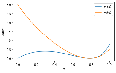
(a) Valuation function of two advertisers.

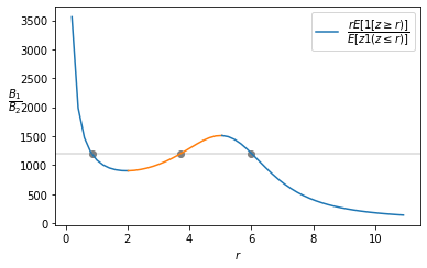
(b) Finding the equilibrium using (3).

Figure 2: An example of two advertisers such that FPA is not AIC (proof of Theorem 4.1). When $\frac{B_{1}}{B_{2}}=1200$, there are three values for $r$ (see the right panel) that lead to equilibrium, and one (orange) leads to non-AIC equilibrium.

So it remains to prove that choosing $f$ as in (8) would result in $g$ as defined in (7). To derive $f$ from $g$, first we simplify $g$ using integration by part,

$$g(r) =\frac{\int_{0}^{r}xf(x)dx}{r\int_{r}^{\infty}f(x)dx}$$

$$=\frac{r\int_{0}^{r}f(x)dx-\int_{0}^{r}\int_{0}^{x}f(y)dydx}{r\int_{r}^{\infty}f(x)dx}$$

$$=\frac{r\int_{0}^{\infty}f(x)dx-\int_{0}^{r}\int_{0}^{x}f(y)dydx}{r\int_{r}^{\infty}f(x)dx}-1,$$

Assuming that $\int_{0}^{\infty}f(x)$ is finite, the above equations lead to the following

$$rg(r)+r=\frac{\int_{0}^{r}\int_{x}^{\infty}f(y)dydx}{\int_{r}^{\infty}f(x)dx}.$$ (9)

Therefore, by integrating the inverse of both sides,

$$\log(\int_{0}^{r}\int_{x}^{\infty}f(y)dydx)=C+\int_{0}^{r}\frac{1}{xg(x)+x}dx,$$

and by raising to the exponent

$$\int_{0}^{r}\int_{x}^{\infty}f(y)dydx=Ke^{\int_{0}^{r}\frac{1}{xg(x)+x}dx}.$$

for some constants $C$ and $K>0$. Then by differentiating both sides with respect to $x$,

$$\int_{r}^{\infty}f(x)dx=\frac{K}{rg(r)+r}e^{\int_{0}^{r}\frac{1}{xg(x)+x}dx}.$$

Note that for any choice of $K\geq 0$, dividing the last two equations will result in (9). So, without loss of generality, we can assume $K=1$. By differentiating again, we can derive $f$ as a function of $g$:

$$f(r)=\frac{(g^{\prime}(r)r+g(r))}{(rg(r)+r)^{2}}e^{\int_{0}^{r}\frac{1}{xg(x)+x}dx}.$$

We need $g^{\prime}(r)r+g(r)\geq 0$ to ensure that $f(r)\geq 0$ for all $r$. This holds for $g$ as in (7). Finally, by substituting $g$ as in (7), we will derive $f$ as in (8). ∎

Remark 4.7.

Note that the above proof shows that for values of $r$ such that there exists a equilibrium which is not AIC, there exists always a second monotone equilibrium. This follows from the fact that the function $g(r)$ tends to infinity as $r\to\infty$, so, $g$ must be increasing for some large enough $r$.

Before moving on to finding conditions for incentive compatibility, we also note that the above’s characterization implies the existence of equilibrium for auto-bidding with any pairs of advertisers.

Proposition 4.8.

Given auto-bidding satisfying the conditions of Lemma 4.4, the equilibrium for all pairs of budgets or all pairs of tCPA constrained advertisers always exists.

Proof.

Recall that the equilibirum exists if there exists an $r$ such that

$$\frac{B_{2}}{B_{1}}=\frac{\int_{0}^{r}xf(x)dx}{r\int_{r}^{\infty}f(x)dx}\vspace{-10pt}$$

has a solution for any value of $\frac{B_{2}}{B_{1}}$. Note that the right-hand side ($\frac{\int_{0}^{r}xf(x)dx}{r\int_{r}^{\infty}f(x)dx}$) is positive for any $r>0$, and it continuously grows to infinity as $r\to\infty$. So, to make sure that every value of $B_{2}/B_{1}$ is covered, we need to check whether at $r=0$ the ratio becomes zero. By L’Hopital rule, $\lim_{z\to 0}\frac{zf(z)}{\int_{z}^{\infty}f(x)dx-zf(z)}=0$, which is as desired.

For tCPA constrained advertiser, the second ratio $\frac{r\int_{0}^{r}f(x)dx}{\int_{r}^{\infty}xf(x)dx}$ always converges to $0$, so the equilibrium in this case always exists. ∎

4.2 Sufficient Conditions for Incentive Compatibility

In this section we show that the lack of ACI happens for cases where advertisers’ valuations have unusual properties. More precisely, the main result of the section is to characterize sufficient conditions on the advertiser’s valuations so that FPA is AIC when there are two advertisers in the auction.

For this goal, we recall the function $f(z)=\frac{v_{2}(h^{-1}(z))}{h^{\prime}(h^{-1}(z))}$ where $h(q)=\frac{v_{1}(q)}{v_{2}(q)}$ defined in Section 4.1. As shown in Lemma4.4, function $f$ behaves as a value of the queries advertiser $2$ gets and the density of queries that advertiser $1$ gets.

Lemma 4.9.

Consider that there are two advertisers and they can either both be budget-advertisers or tCPA-advertisrs. Also, suppose that auto-bidder with FPA uses the optimal bidding strategy in Claim 4.3. Then a sufficient condition for FPA to be AIC is that $f$ has a monotone hazard rate, i.e., $\frac{f(r)}{\int_{r}^{\infty}f(x)dx}$ is non-decreasing in $r$.

Proof.

Following the proof Theorem 4.1, if $g(r)=\frac{\int_{0}^{r}\int_{x}^{\infty}f(y)dydx}{r\int_{r}^{\infty}f(x)dx}$ is non-decreasing in $r$ then the equilibrium is AIC. The equivalent sufficient conditions obtained by imposing the inequality $g^{\prime}(r)\geq 0$ is that for all $r\geq 0$,

$$r\big{(}\int_{r}^{\infty}f(x)dx\big{)}^{2}\geq\big{(}\int_{0}^{r}\int_{x}^{\infty}f(y)dydx\big{)}\big{(}\int_{r}^{\infty}f(x)dx-rf(r)\big{)}.$$ (10)

If $\int_{r}^{\infty}f(x)dx\leq rf(r)$ then above’s inequality obviously holds. So, we can assume that for some $r>0$, $\int_{r}^{\infty}f(x)dx>rf(r)$. Since $\frac{f(z)}{\int_{z}^{\infty}f(x)dx}$ is non-decreasing in $z$, we must have that for all $r^{\prime}\leq r$, $\frac{f(r^{\prime})}{\int_{r^{\prime}}^{\infty}f(x)dx}\leq\frac{f(r)}{\int_{r}^{\infty}f(x)dx}\leq\frac{1}{r}\leq\frac{1}{r^{\prime}}$. On the other hand by taking the derivative of $\frac{f(z)}{\int_{z}^{\infty}f(x)dx}$, we must have that $f^{\prime}(z)\int_{z}^{\infty}f(x)dx+f(z)^{2}\geq 0$. By considering two cases on the sign of $f^{\prime}$, for $z\leq r$ we must have, $f(z)\big{(}zf^{\prime}(z)+f(z))\geq 0$, and hence $(zf(z))^{\prime}\geq 0$ for all $z\leq r$. Therefore, $zf(z)$ is non-decreasing for $z\leq r$.

On the other hand,

$$\int_{0}^{r}\int_{x}^{\infty}f(y)dydx =\int_{0}^{r}\int_{x}^{r}f(y)dydx+\int_{0}^{r}\int_{r}^{\infty}f(y)dydx$$

$$=r\int_{0}^{r}f(x)dx-\int_{0}^{r}\int_{0}^{x}f(y)dydx+r\int_{r}^{\infty}f(x)dx$$

$$=\int_{0}^{r}xf(x)dx+r\int_{r}^{\infty}f(x)dx,$$

where the second equation is by integration by part. Then by applying monotonicity of $z(f)z$ for $z\leq r$ we have $\int_{0}^{r}\int_{x}^{\infty}f(y)dydx\leq r^{2}f(r)+r\int_{r}^{\infty}f(x)dx$. So, to prove (10) it is enough to show that

$$\left(\int_{r}^{\infty}f(x)dx\right)^{2}\geq\left(rf(r)+\int_{r}^{\infty}f(x)dx\right)\left(\int_{r}^{\infty}f(x)dx-rf(r)\right),$$

which holds, since the right-hand side is equal to $\big{(}\int_{r}^{\infty}f(x)dx\big{)}^{2}-(rf(r))^{2}$ strictly less than the left-hand side. ∎

While the condition on $f$ has intuitive properties when seen as a density, it has the unappealing properties to be too abstract in terms of the conditions on the advertisers’ valuation. The following result, provides sufficient conditions on value functions $v_{1}$ and $v_{2}$ that makes $f$ be monotone hazard rate, and hence, FPA to be AIC.

Theorem 4.10.

Consider two advertisers that are either budget-advertisers or tCPA-advertisers. Assume that $h(q)=\frac{v_{1}(q)}{v_{2}(q)}$ is increasing concave function and that $v_{2}$ is non-decreasing. Then, the equilibrium in FPA auto-bidding with bidding strategy as in Claim 4.3 is AIC.

Proof.

Note that when $f$ is non-decreasing, it also has a monotone hazard rate. Now, when $h$ is concave, $\frac{1}{h^{\prime}}$ is a non-decreasing function, and since $v_{2}$ is also non-decreasing, then $f$ is also non-decreasing. ∎

4.3 FPA with uniform bidding

The previous section shows that when auto-bidders have full flexibility on the bidding strategy, FPA is not AIC. However, non-uniform bid is not simple to implement and auto-bidders may be constrained to use simpler uniform bidding policies (aka pacing bidding). In this context, the main result of the section is Theorem 4.2 that shows that when restricted to uniform bidding policies FPA is AIC. Note that here, we are assuming a simple model where advertisers do not split campaigns. So, FPA with uniform bidding is AIC but it could bring up other incentives for advertisers when it is implemented.

Definition 4.11 (Uniform bidding equilibrium).

A uniform bidding equilibrium for the auto-bidders subgame corresponds to bid multipliers $\mu_{1},\ldots,\mu_{N}$ such that every auto-bidder $a$ chooses the uniform bidding policy $\mu_{a}$ that maximizes Problem (1) when restricted to uniform bidding policies with the requirement that if advertiser $a$’s constraints of type 2 are not tight then $\mu_{a}$ gets its maximum possible value.

The proof of Theorem 4.2 is based on the main results of Conitzer et al. (2022a). The authors proved that the uniform-bidding equilibrium is unique and in equilibrium the multiplier of each advertiser is the maximum multiplier over all feasible uniform bidding strategies. Their result is for budget-constrained advertisers, and we extend it to include tCPA constrained advertisers. The proof is deferred to Appendix B.

Lemma 4.12 (Extension of Theorem 1 in Conitzer et al. (2022a)).

Given an instance of Auto-bidding with general constraints as in (2), there is a unique uniform bidding equilibrium, and the bid multipliers of all advertisers is maximal among all feasible uniform bidding profiles.

Now, we are ready to prove Theorem 4.2.

Proof of Theorem 4.2.

Assume that advertiser $1$ increases their budget or their target CPA. Then the original uniform bidding is still feasible for all advertisers. Further, by Lemma 4.12 the equilibrium pacing of all advertisers is maximal among all feasible pacings. So, the pacing of all advertisers will either increase or remain the same. But the constraints of all advertisers except 1 are either binding or their multiplier has attained its maximum value by the definition of pacing equilibrium. Therefore, the set of queries they end up with should be a subset of their original ones since the price of all queries will either increase or remain the same. So, it is only advertiser 1 that can win more queries. ∎

Remark 4.13.

Conitzer et al. (2022a) show monotonicity properties of budgets in FPA with uniform bidding equilibrium for the revenue and welfare. Instead, in our work we focus on monotonicity for each advertiser.

5 Truthful Auctions

This section studies auto-bidding incentive compatibility for the case where the per-query auction is a truthful auction.

A truthful auction is an auction where the optimal bidding strategy for a profit-maximizing agent is to bid its value. An important example of a truthful auction is Second Price Auction. As we showed in the three-queries example of the introduction, SPA is not AIC. In this section, we show that the previous example generalizes, in our continuous-query model, to any (randomized) truthful auctions so long as the auction is scalar invariant and symmetric (see Assumption 5.1 below for details). As part of our proof-technique, we obtain an auction equivalence result which is interesting on its own: in the continuous query-model SPA and FPA have the same outcome.

For the remaining of the section we assume all truthful auction satisfy the following property.

Assumption 5.1.

Let $(x_{a}(\mathbf{b}))_{a\in A}$ be the allocation rule in a truthful auction given bids $\mathbf{b}=(b_{a})_{a\in A}$. We assume that the allocation rule satisfies the following properties.

1. The auction always allocates: $\sum_{a\in A}x_{a}(\mathbf{b})=1$

2. Scalar invariance: For any constant $c>0$ and any advertiser $a\in A$, $x_{a}(\mathbf{b})=x_{a}(c\mathbf{b})$.

3. Symmetry: For any pair of advertisers $a,a^{\prime}\in A$ and bids $b,b^{\prime},\mathbf{b}_{-\{a,a^{\prime}\}}=(b)_{a\in A\setminus\{a,a^{\prime}\}}$ we have that

   $$x_{a}(b_{a}=b,b_{a^{\prime}}=b^{\prime},\mathbf{b}_{-\{a,a^{\prime}\}})=x_{a^{\prime}}(b_{a}=b^{\prime},b_{a^{\prime}}=b,\mathbf{b}_{-\{a,a^{\prime}\}}).$$

Remark 5.2.

Observe that SPA satisfies Assumption 5.1.

From the seminal result of Myerson (1981) we obtain a tractable characterization of truthful auctions which we use in our proof.

Lemma 5.3 (Truthful auctions (Myerson, 1981)).

Let $(x_{a}(\mathbf{b}),p_{a}(\mathbf{b}))_{a\in A}$ the allocation and pricing rule for an auction given bids $\mathbf{b}=(b_{a})_{a\in A}$. The auction rule is truthful if and only if

1. Allocation rule is non-decreasing on the bid: For each bidder $a\in A$ and any $b_{a}^{\prime}\geq b_{a}$, we have that

   $$x_{a}(b^{\prime}_{a},\mathbf{b}_{-a})\geq x_{a}(b_{a},\mathbf{b}_{-a}).$$

2. Pricing follows Myerson’s formulae:

   $$p_{a}(\mathbf{b})=b_{a}\cdot x_{a}(\mathbf{b})-\int_{0}^{b_{a}}x_{a}(z,\mathbf{b}_{-a})dz.$$

A second appealing property of truthful actions is that the optimal bidding strategy for auto-bidders is simpler: in the discrete-query model uniform bidding strategy is almost optimal and can differ from optimal by at most the value of two queries (Aggarwal et al., 2019). We revisit this result in our continuous-query model and show that uniform bidding policy is optimal for truthful auctions.

Claim 5.4.

In the continuous-query model, if the per-quuery auction is truthful then using a uniform bidding is an optimal strategy for each auto-bidder.

Proof.

We use Theorem 1 Aggarwal et al. (2019). Pick some small $\delta>0$ and divide the interval $[0,1]$ into subintervals of length $\delta$. Let each subinterval $I$ be a discrete query with value functions $v_{j}(I)=\int_{I}v_{j}(q)dq$. Then Theorem 1 Aggarwal et al. (2019) implies that uniform bidding differs from optimal by at most two queries. So, the difference from optimal is bounded by $2\max_{j}\max_{|I|\leq\delta}v_{j}(I)$. Now, since the valuation functions are atomless (i.e., the value of a query is $dq$), by letting $\delta$ to $0$, the error of uniform bidding in the continuous case also goes to zero. ∎

5.1 SPA in the Continuous-Query Model

We generalize the discrete example of second price auction in Theorem 2.1 to the continuous set of queries model showing that SPA is not AIC. The key step consists on showing that for the continuous-query model there is an auction equivalence result between first and second price auction.

Theorem 5.5.

[Auction Equivalence Result] Suppose that auto-bidder uses a uniform bid strategy for SPA, and similarly, uses the simple bidding strategy defined in Claim 4.3 for FPA. Then, in any subgame equilibrium the outcome of the auctions (allocations and pricing) on SPA is the same as in FPA.

This result immediately implies that all the results for FPA in Section 4 hold for SPA as well.

Theorem 5.6.

Suppose that there are at least two budget-advertisers or two tCPA-advertisers, then even for the continuous-query model SPA is not AIC.

Similarly to FPA case, we can characterize the equilibrium for the two-advertiser case and derive sufficient conditions on advertisers’ valuation functions so that SPA is AIC.

Theorem 5.7.

Given two advertisers, let $\mu_{1}$ and $\mu_{2}$ be the bidding multipliers in equilibrium for the subgame of the auto-bidders. Also assume that $h(q)=\frac{v_{1}(q)}{v_{2}(q)}$ is increasing. Then

1. If the advertisers are budget-constrained with budget $B_{1}$ and $B_{2}$, then $\mu_{1}=\frac{B_{2}}{E[z\mathbbm{1}(z\geq r)]}$ and $\mu_{2}=\mu_{1}r$, where $r$ is the answer of the following implicit function,

   $$\frac{rE[\mathbbm{1}[z\geq r)]}{E[z\mathbbm{1}(z\leq{r})]}=\frac{B_{1}}{B_{2}}.$$

   Here, $E[.]$ is defined as $E[P(z)]=\int_{0}^{\infty}P(z)f(z)dz,$ where $f(z)=\frac{v_{2}(h^{-1}(z))}{h^{\prime}(h^{-1}(z))}$ wherever $h^{\prime}$ is defined, and it is zero otherwise.

2. If the advertisers are tCPA-constrained with targets $T_{1}$ and $T_{2}$, we have $\mu_{1}=\frac{T_{1}E[\mathbbm{1}(z\leq r)]}{E[\mathbbm{1}(z\geq r)]}$ and $\mu_{2}=\mu_{1}r$, where $r$ is the answer of the following implicit function,

   $$\frac{rE[\mathbbm{1}(z\geq r)]}{E[z\mathbbm{1}(z\geq{r})]}\frac{E[\mathbbm{1}(z\leq r)]}{E[z\mathbbm{1}(z\leq{r})]}=\frac{T_{1}}{T_{2}}.$$

3. If further, $v_{2}$ is non-decreasing in $q$, and $h$ is concave, and advertiers are either both budget-constrained two tCPA-constrained, then SPA is AIC.

We now demonstrate the auction equivalence between FPA and SPA.

Proof of Theorem 5.5.

Note that the optimal strategy for a second-price auction is uniform bidding with respect to the true value of the query by Claim 5.4. Also, Claim 4.3 implies that the cost obtained by each advertiser in first-price auction in the continuous model is also depends on pacing multipliers of the other advertiser. This claim immediately, suggests the equivalent between the optimal. bidding strategies of first and second price auctions. So, the optimal strategy for both auctions will be the same and therefore the resulting allocation and pricing will also be the same. Hence, it follows that the same allocation and pricing will be a pure equilibrium under both auctions. ∎

5.2 Truthful Auctions Beyond Second-Price

We now present the main result of the section. We show that a general truthful auction (with possibly random allocation) is not AIC.

Theorem 5.8.

Consider a truthful auction $(\mathbf{x},\mathbf{p})$ satisfying Assumption 5.1. If there are at least two budget-advertisers or two tCPA-advertisers, then the truthful auction is not AIC.

The remainder of the section gives an overview of the proof of this theorem. Similar to the FPA and SPA case, we start by characterizing the equilibrium in the continuous case when there are two advertisers in the game. The proof relies on the observation that for auctions satisfying Assumption 5.1, the allocation probability is a function of the bids’ ratios. So, again, similar to FPA and SPA finding the equilibrium reduces to finding the ratio of bidding multipliers. Then to finish the proof of Theorem 5.8 instead of providing an explicit example where auto-bidding is non-AIC, we showed that the conditions needed for an auction’s allocation probability to satisfy are impossible.

The following theorem finds an implicit equation for the best response. We omit the proofs of the intermediaries steps and deferred them to the Appendix C.

Theorem 5.9.

Consider a truthful auction $(\mathbf{x},\mathbf{p})$ satisfying Assumption 5.1 and assume that there are either two budget-advertisers or two tCPA-advertisers. Let $\mu_{1}$ and $\mu_{2}$ be the bidding multipliers used by the auto-bidders in the subgame equilibrium. Further, assume that $h(q)=\frac{v_{1}(q)}{v_{2}(q)}$ is increasing. Then

1. If the advertisers are budget-constrained with budget $B_{1}$ and $B_{2}$, then $\mu_{1}=\frac{B_{1}}{E[p_{1}(rz,1)]}$ and $\mu_{2}=r\mu_{1}$, where $r$ is the answer of the following implicit function,

   $$\frac{E[rp_{1}(\frac{z}{r},1)]}{E[zp_{1}(\frac{r}{z},1)]}=\frac{B_{1}}{B_{2}}.$$

   Here, $E[.]$ is defined as $E[P(z)]=\int_{0}^{\infty}P(z)f(z)dz,$ where $f(z)=\frac{v_{2}(h^{-1}(z))}{h^{\prime}(h^{-1}(z))}$ wherever $h^{\prime}$ is defined, and it is zero otherwise.

2. If the advertisers are tCPA-constrained with targets $T_{1}$ and $T_{2}$, we have $\mu_{1}=\frac{T_{1}E[zg(z/r)]}{E[rp_{1}(z/r)]}$ and $\mu_{2}=\mu_{1}r$, where $r$ is the answer of the following implicit function,

   $$\frac{E[x_{1}(\frac{r}{z},1)]}{E[zx_{1}(\frac{z}{r},1)]}\frac{E[rp_{1}(\frac{z}{r},1)]}{E[zp_{1}(\frac{r}{z},1)]}=\frac{T_{1}}{T_{2}}.$$

Because allocation probability $x_{1}$ is a non-decreasing function, we can derive a similar result to the FPA case and show if an instance is not AIC for budget-advertisers then it is also not AIC for tCPA-advertisers.

Proposition 5.10.

If for the two budget-constrained advertisers case the truthful auction is not AIC, then for the tCPA-constrained advertisers case the same auction is also not AIC.

Using the previous results we are in position to tackle the main theorem.

Proof of Theorem 5.8.

We prove Theorem 5.8 for budget constrained advertisers, since Proposition 5.10 would derive it for tCPA constraint advertisers. We use implicit function theorem to find conditions on $p_{1}$ and $f$ to imply monotonicity in $r$. Let

$$H(x,r)=\frac{\int_{0}^{\infty}rf(z)p_{1}(z/r,1)dz}{\int_{0}^{\infty}f(z)zp_{1}(r/z,1)dz}-x.$$

Then when advertiser $1$ increases budget, the corresponding variable $x$ increases. So, if we want to check whether $r$ is a non-decreasing function of $x$, we need $\frac{dr}{dx}$ to be non-negative. By the implicit function theorem,

$$\frac{dr}{dx}=-\frac{\frac{\partial H}{\partial x}}{\frac{\partial H}{\partial r}}=\frac{1}{\frac{\partial H}{\partial r}}.$$

So, assume to the contrary that $r$ i always non-decreasing in x, then $\frac{\partial H(x,r}{\partial r}\geq 0$. Define $p(x)=p_{1}(x,1)$. Then we have the following

$$E[\frac{d}{dr}rp(z/r)]E[zp(r/z)]\geq E[rp(z/r)]E[\frac{d}{dr}\Big{(}zp(r/z)\Big{)}].$$

Then

$$\frac{\frac{d}{dr}E[rp(z/r)]}{E[rp(z/r)]}\geq\frac{\frac{d}{dr}E[zp(z/r)]}{E[zp(z/r)]}$$

By integrating both parts, we have that for any choice of $f$,

$$rE[p(z/r)]\geq E[zp(r/z)].$$

When the above inequality hold for any choice of $v_{1}$ and $v_{2}$, we claim that the following must hold almost everywhere

$$p(b)\geq bp(1/b).$$ (11)

To see this, assume to the contrary that there exist a measurable set $B$ such that (11) does not hold for it. Let $qv_{2}(q)=v_{1}(q)$, therefore, $f(z)=v_{2}(z)$ can be any measurable function. So, we can define $f$ to have zero value everywhere except $X$, and have weight 1 over $X$ to get a contradiction.

By substituting variable with $y=1/b$ in (11), $p(1/b)db\geq p(b)/bdb$. Therefore, almost everywhere $p(b)=bp(1/b)$. By differentiating we have $p^{\prime}(b)=p(1/b)-p^{\prime}(1/x)/x$. On the other hand, as we will see in Appendix C for any truthful auction satisfying Assumption 5.1, $p^{\prime}(b)=p^{\prime}(1/b)$. Therefore, $p(b)=p^{\prime}(b)(b+1)$. Solving it for $p$, we get that the only possible AIC pricing must be of the form $p(b)=\alpha(b+1)$ for some $\alpha>0$.

Next, we will show there is no proper allocation probability satisfying the Assumption 5.1 that would result in a pricing function $p$. It is not hard to see that by the Myerson’s pricing formulae, $\frac{dx_{1}(b,1)}{db}=\frac{p^{\prime}(b)}{b}.$ Therefore, we must have $x_{1}^{\prime}(b,1)=\alpha/b$, so $x_{1}(b,1)=c\log(b)+d$ for some constants $c>0$ and $d$. But $x_{1}$ cannot be a valid allocation rule, since it will take negative values for small enough $b$. ∎

Appendix A Second-price tCPA constrained

Proof.

We continue with the proof of Theorem 2.1. We first prove the uniqueness of equilibrium in the case of $B_{1}^{\prime}=1$. irst, note that there’s no equilibrium such that advertiser 1 wins all the queries. To see this, note that the multiplier of advertiser 1 is at most $1$. Hence, the price of $q_{3}$ for advertiser 2 is within their budget, and they have the incentive to increase their multiplier to buy $q_{3}$. Similarly, one can see that in any equilibrium, advertiser 1 gets at least $q_{1}$, since its highest price is within their budget.

Now, assume some equilibrium exists with bidding prices $\tilde{\mu}_{1}$ and $\tilde{\mu}_{2}$ such that advertiser 1 gets only $q_{1}$. Then

$$\frac{\tilde{\mu}_{1}(v_{1}(1)+v_{1}(2)+v_{1}(3))}{B_{2}}>1\geq\frac{\tilde{\mu}_{2}v_{2}(1)}{B_{1}},$$

where the first inequality is because advertiser 2’s multiplier is the best response, and the second is coming from the budget constraint for advertiser 1. Therefore,

$$\frac{B_{1}}{B_{2}}\frac{v_{1}(1)+v_{1}(2)+v_{1}(3)}{v_{2}(1)}\geq\frac{\tilde{\mu}_{2}}{\tilde{\mu}_{1}},$$

But $\frac{v_{1}(2)}{v_{2}(2)}\geq\frac{B_{1}}{B_{2}}\frac{v_{1}(1)+v_{1}(2)+v_{1}(3)}{v_{2}(1)}=\frac{9}{4}$, and thus $\frac{v_{1}(2)}{v_{2}(2)}>\frac{\tilde{\mu}_{2}}{\tilde{\mu}_{1}}$. This is in contradiction with allocation inequalities since advertiser 2 wins $q_{2}$. Therefore, we proved with $B_{1}=1$ and $B_{2}=4$ the equilibrium is unique such that advertiser 1 wins $q_{1}$ and $q_{2}$.

Now it remains to show a non AIC example for tCPA advertisers. Again consider two advertisers, and 3 queries, with the same values as in Table 2. Here, let the tCPA constraint of advertiser 1 be $T_{1}=0.4$ and for advertiser 2 be $T_{2}=0.7$. Then again we show that there exists a unique equilibrium in which advertiser 1 gets queries 1 and 2.

First, to prove the existence, let $\mu_{1}=1.6$ and $\mu_{2}=1.2$. Then we show this is an equilibrium since the three following conditoins hold:

1. Allocation: advertiser 1 wins $q_{1}$ and $q_{2}$ since it has a higher bid on them

   $$\frac{v_{1}(1)}{v_{2}(1)}\geq\frac{v_{1}(2)}{v_{2}(2)}\geq\frac{\mu_{2}}{\mu_{1}}=\frac{1.2}{1.5}\geq\frac{v_{1}(3)}{v_{2}(3)}.$$

2. tCPA constraints are satisfied:

   $$T_{2}v_{2}(3)\geq\mu_{1}v_{1}(3),\qquad\text{and }$$

   $$T_{1}(v_{1}(1)+v_{1}(2))\geq\mu_{2}(v_{2}(1)+v_{2}(2)).$$

3. Best response: non of the advertiser can win more queries if they increase their multiplier:

   $$T_{2}(v_{2}(3)+v_{2}(2))<\mu_{1}(v_{1}(3)+v_{1}(2)),\qquad\text{and}$$

   $$T_{1}(v_{1}(1)+v_{1}(2)+v_{1}(3))<\mu_{2}(v_{2}(1)+v_{2}(2)+v_{2}(3)).$$

Now, similar to the proof of the budget-constrained advertisers we show the equilibrium is unique. Note that there’s no equilibrium such that advertiser 1, gets all queries since the cost of all queries for advertiser 1 is at least $v_{2}(1)+v_{2}(2)+v_{2}(3)=12.3$ which is larger than $T_{1}(v_{1}(1)+v_{1}(2)+v_{1}(3))$. Similarly, advertiser 2 cannot get all queries since the tCPA constraint would not hold $v_{1}(1)+v_{1}(2)+v_{1}(3)>T_{2}(v_{2}(1)+v_{2}(2)+v_{2}(3))$. So, to prove the uniqueness of equilibrium, it remains to show that there’s no equilibrium that advertiser 1 only gets query 1. To contradiction, assume such equilibrium exists with the corresponding multipliers $\tilde{\mu}_{1}$ and $\tilde{\mu}_{2}$. Then we must have

$$\frac{\tilde{\mu}_{1}(v_{1}(1)+v_{1}(2)+v_{1}(3))}{T_{2}(v_{2}(1)+v_{2}(2)+v_{2}(3))}>1\geq\frac{\tilde{\mu}_{2}v_{2}(1)}{T_{1}v_{1}(1)},$$

where the first inequality is because advertiser 2’s multiplier is the best response, and the second inequality is coming from the budget constraint for advertiser 1. Therefore,

$$\frac{T_{1}}{T_{2}}\frac{v_{1}(1)+v_{1}(2)+v_{1}(3)}{v_{2}(1)+v_{2}(2)+v_{2}(3)}\frac{v_{1}(1)}{v_{2}(1)}\geq\frac{\tilde{\mu}_{2}}{\tilde{\mu}_{1}},$$

But $\frac{v_{1}(2)}{v_{2}(2)}\geq\frac{T_{1}}{T_{2}}\frac{v_{1}(1)+v_{1}(2)+v_{1}(3)}{v_{2}(1)+v_{2}(2)+v_{2}(3)}\frac{v_{1}(1)}{v_{2}(1)}$, and thus $\frac{v_{1}(2)}{v_{2}(2)}>\frac{\tilde{\mu}_{2}}{\tilde{\mu}_{1}}$. This is in contradiction with allocation inequalities since advertiser 2 wins $q_{2}$. Therefore, we proved with $T_{1}=0.4$ and $T_{2}=0.7$, the equilibrium is unique such that advertiser 1 wins $q_{1}$ and $q_{2}$.

Now, we show that if advertiser 1 increases their tCPA constraint to $T^{\prime}_{1}=0.6$, then there exists an equilibrium such that advertiser 1 only wins $q_{1}$. Let $\mu_{1}^{\prime}=1$ and $\mu_{2}=2.38$. Then

1. Allocation: advertiser 1 wins $q_{1}$

   $$\frac{v_{1}(1)}{v_{2}(1)}\geq\frac{\mu^{\prime}_{2}}{\mu^{\prime}_{1}}=\frac{2.38}{1.}\geq\frac{v_{1}(2)}{v_{2}(2)}\geq\frac{v_{1}(3)}{v_{2}(3)}.$$

2. tCPA constraints are satisfied:

   $$T_{2}(v_{2}(3)+v_{2}(2))\geq\mu^{\prime}_{1}(v_{1}(3)+v_{1}(2)),\qquad\text{and }$$

   $$T_{1}^{\prime}v_{1}(1)\geq\mu_{2}^{\prime}v_{2}(1).$$

3. Best response: non of the advertiser can win more queries if they increase their multiplier:

   $$T_{2}(v_{2}(1)+v_{2}(2)+v_{2}(3))<\mu_{1}^{\prime}(v_{1}(1)+v_{1}(2)+v_{1}(3)),\qquad\text{and}$$

   $$T^{\prime}_{1}(v_{1}(1)+v_{1}(2))<\mu_{2}^{\prime}(v_{2}(1)+v_{2}(2)).$$

   ∎

∎

Appendix B First-price pacing equilibrium

Proof of Lemma 4.12.

We follow the same steps of the proof as in Conitzer et al. (2022a) for tCPA constrained advertisers. Consider two sets of feasible bidding multipliers $\mathbf{\mu}$ and $\mathbf{\mu}^{\prime}$. We will show that $\mathbf{\mu}^{*}=\max(\mathbf{\mu},\mathbf{\mu}^{\prime})$ is also feasible, where $\max$ is the component wise maximum of the bidding profiles for $n$ advertisers.

Each query $q$ is allocated to the bidder with the highest pacing bid. We need to check that constraint (2) is satisfied. Fix advertiser $a$. Its multiplier in $\mathbf{\mu}^{*}$ must be also maximum in one of $\mathbf{\mu}$, or $\mathbf{\mu}^{\prime}$. without loss assume $\mu^{*}_{a}=\mu_{a}$. Then the set of queries that $a$ wins with bidding profile $\mathbf{\mu}^{*}$ ($X^{*}_{a}$) must be a subset of queries it wins n $\mathbf{\mu}$ ($X_{a}$), since all other advertisers’ bids have either remained the same or increased. On the other hand, the cost of queries $a$ wins stays the same, since it’s a first price auction. Since constraint (2) is feasible for bidding multipliers $\mathbf{\mu}$ we must have

$$(\mu_{a}-T_{a})\int_{q\in X}v_{a}(q)\leq B_{a}.$$

But then since $X^{*}\subseteq X$, we have as well

$$(\mu_{a}-T_{a})\int_{q\in X^{*}}v_{a}(q)=(\mu_{a}^{*}-T_{a})\int_{q\in X^{*}}v_{a}(q)\leq B_{a},$$

which implies $\mathbf{\mu}^{*}$ is a feasible strategy.

To complete the proof we need to show the strategy that all advertisers take the maximum feasible pace $\mu^{*}_{a}=\sup\{\mu_{a}|\mu\text{ is feasible}\}$ results in an equilibrium. To see this, note that if an advertiser’s strategy is not best-response, they have incentive to increase their pace with its constraints remaining satisfied. But then this would result into another feasible pacing strategy and is in contradiction with the choice of the highest pace $\mu_{a}^{*}$. A similar argument also shows the equilibrium is unique. Assume there exists another pacing equilibrium where an advertiser $a$ exists such that its pace is less than $\mu^{*}_{a}$. Then by increasing their pace to $\mu_{a}^{*}$ they will get at least as many queries as before, so $\mu_{a}^{*}$ is the best-response strategy. ∎

Appendix C Proofs for Truthful Auctions

We start by the following observation, which follows by applying Assumption 5.1 to reformulate the allocation function in the case of two advertisers as a function of a single variable.

Claim C.1.

The probability of allocating each query is a function of the ratio of bids, i.e., there exists a non-decreasing function $g:\mathbb{R}^{+}\to[0,1]$ such that the followings hold.

1. $x_{1}(b_{1}(q),b_{2}(q))=g(\frac{b_{1}(q)}{b_{2}(q)})$,

2. $g(z)+g(1/z)=1$,

3. $g(0)=0$.

For example, SPA satisfies the above claim with $g(z)=1$ when $z=\frac{b_{1}(q)}{b_{2}(q)}\geq 1$. We are ready to prove Theorem 5.9, which follows the similar steps of Lemma 4.4.

Proof of Theorem 5.9.

By Claim 5.4, there exists $\mu_{1}$ and $\mu_{2}$ such that advertiser $a$ bids $z_{a}v_{a}(q)$ on each query. Therefore, we can write the budget constraint for bidder 1 as,

$$B_{1}=\int_{0}^{1}p_{1}(b_{1}(q),b_{2}(q))dq=\int_{0}^{1}\mu_{1}v_{1}(q)g\Big{(}\frac{v_{1}(q)}{v_{2}(q)}\frac{\mu_{1}}{\mu_{2}}\Big{)}dq-\int_{0}^{1}\int_{0}^{\mu_{1}v_{1}(q)}g\Big{(}\frac{x}{v_{2}(q)\mu_{2}}\Big{)}dxdq$$

Next, with a change of variable $x=v_{1}(q)y$ we have

$$B_{1}=\int_{0}^{1}\mu_{1}v_{1}(q)g\Big{(}\frac{v_{1}(q)}{v_{2}(q)}\frac{\mu_{1}}{\mu_{2}}\Big{)}dq-\int_{0}^{1}\int_{0}^{\mu_{1}}g\Big{(}\frac{v_{1}(q)}{v_{2}(q)\mu_{2}}y\Big{)}{v_{1}(q)}dydq.$$

As before, let $h(q)=\frac{v_{1}(q)}{v_{2}(q)}$. Then let $z=h(q)$, we have $dq=dh^{-1}(z)=\frac{1}{h^{\prime}(h^{-1}(z))}dz$. So,

$$B_{1}=\int_{0}^{\infty}\mu_{1}v_{1}(h^{-1}(z))g\Big{(}\frac{z\mu_{1}}{\mu_{2}}\Big{)}\frac{1}{h^{\prime}(h^{-1}(z))}dz-\int_{0}^{\infty}\int_{0}^{\mu_{1}}g\Big{(}\frac{z}{\mu_{2}}y\Big{)}{v_{1}(h^{-1}(z))}dy\frac{1}{h^{\prime}(h^{-1}(z))}dz.$$

Define $f(z)=\frac{v_{2}(h^{-1}(z))}{h^{\prime}(h^{-1}(z))}=\frac{1}{z}\frac{v_{1}(h^{-1}(z))}{h^{\prime}(h^{-1}(z))}$. Then we have

$$B_{1}=\int_{0}^{\infty}\mu_{1}zf(z)g\Big{(}\frac{z\mu_{1}}{\mu_{2}}\Big{)}dz-\int_{0}^{\infty}\Big{(}\int_{0}^{\mu_{1}}g\Big{(}\frac{z}{\mu_{2}}y\Big{)}dy\Big{)}zf(z)dz.$$

Similarly,

$$B_{2}=\int_{0}^{\infty}\mu_{2}v_{2}(h^{-1}(z))(1-g\Big{(}\frac{z\mu_{1}}{\mu_{2}}\Big{)})\frac{1}{h^{\prime}(h^{-1}(z))}dz-\int_{0}^{\infty}\int_{0}^{\mu_{2}}g\Big{(}\frac{y}{\mu_{1}z}\Big{)}{v_{2}(h^{-1}(z))}dy\frac{1}{h^{\prime}(h^{-1}(z))}dz.$$

$$B_{2}=\int_{0}^{\infty}\mu_{2}f(z)(1-g\Big{(}\frac{z\mu_{1}}{\mu_{2}}\Big{)})dz-\int_{0}^{\infty}\int_{0}^{\mu_{2}}g\Big{(}\frac{y}{\mu_{1}z}\Big{)}dyf(z)dz.$$

Next, we find the implicit function to derive $r=\frac{\mu_{2}}{\mu_{1}}$. By change of variable we have the following two equations:

$$\frac{B_{1}}{\mu_{1}}=\int_{0}^{\infty}zf(z)g(z/r)dz-r\int_{0}^{\infty}\Big{(}\int_{0}^{z/r}g(w)dw\Big{)}f(z)dz.$$

$$\frac{B_{2}}{\mu_{2}}=\int_{0}^{\infty}f(z)(1-g(z/r))dz-\frac{1}{r}\int_{0}^{\infty}\Big{(}\int_{0}^{r/z}g(w)dw\Big{)}zf(z)dz.$$

The implicit function for $r$ is the following:

$$\frac{B_{1}}{B_{2}}=\frac{\int_{0}^{\infty}f(z)\Big{(}zg(z/r)-r\int_{0}^{z/r}g(w)dw\Big{)}dz}{\int_{0}^{\infty}f(z)\Big{(}r(1-g(z/r)-z\int_{0}^{r/z}g(w)dw\Big{)}dz}.$$

Recall the payment rule in Assumption 5.3, this can be re-written as

$$\frac{B_{1}}{B_{2}}=\frac{\int_{0}^{\infty}rf(z)p_{1}(z/r,1)dz}{\int_{0}^{\infty}zf(z)zp_{1}(r/z,1)dz},$$

which finishes the proof for the budget constrained advertisers.

Now, consider two tCPA constrained advertisers. Following the same argument as above, we get the following from tightness of tCPA constraints

$$T_{1}\int_{0}^{\infty}zf(z)g\Big{(}\frac{z\mu_{1}}{\mu_{2}}\Big{)}dz=\int_{0}^{\infty}\mu_{1}zf(z)g\Big{(}\frac{z\mu_{1}}{\mu_{2}}\Big{)}dz-\int_{0}^{\infty}\Big{(}\int_{0}^{\mu_{1}}g\Big{(}\frac{z}{\mu_{2}}y\Big{)}dy\Big{)}zf(z)dz,$$

and,

$$T_{2}\int_{0}^{\infty}f(z)(1-g\Big{(}\frac{z\mu_{1}}{\mu_{2}}\Big{)})dz=\int_{0}^{\infty}\mu_{2}f(z)(1-g\Big{(}\frac{z\mu_{1}}{\mu_{2}}\Big{)})dz-\int_{0}^{\infty}\int_{0}^{\mu_{2}}g\Big{(}\frac{y}{\mu_{1}z}\Big{)}dyf(z)dz.$$

By dividing both sides of the equations we get the desired results. ∎

Now, to prove the main theorem, we need to show that the values accrued by advertisers is monotone in $\mu_{1}/\mu_{2}$.

Claim C.2.

Let $\mu_{i}$ be the optimal bidding multiplier for advertiser $i$. Given the assumptions in Theorem 5.8, the value obtained by advertiser $1$ is increasing in $r=\frac{\mu_{1}}{\mu_{2}}$.

Proof.

Following the proof of Theorem 5.9 we can write value obtained by advertiser $i$ as

$$V_{1}(B_{1},B_{2})=\int_{0}^{\infty}f(z)zg(rz)dz,$$

where $r$ is the answer to the implicit function stated in Theorem 5.9. Monotonicity of $V_{1}(B_{1},B_{2})$ as a function of $r$ follows from the fact that $g$ is a monotone function. ∎

References

- (1)
- Aggarwal et al. (2019) Gagan Aggarwal, Ashwinkumar Badanidiyuru Varadaraja, and Aranyak Mehta. 2019. Autobidding with Constraints. In Web and Internet Economics 2019.
- Allouah and Besbes (2020) Amine Allouah and Omar Besbes. 2020. Prior-independent optimal auctions. Management Science 66, 10 (2020), 4417–4432.
- Balseiro et al. (2021a) Santiago Balseiro, Yuan Deng, Jieming Mao, Vahab Mirrokni, and Song Zuo. 2021a. Robust Auction Design in the Auto-bidding World. In Advances in Neural Information Processing Systems, M. Ranzato, A. Beygelzimer, Y. Dauphin, P.S. Liang, and J. Wortman Vaughan (Eds.), Vol. 34. Curran Associates, Inc., 17777–17788. https://proceedings.neurips.cc/paper/2021/file/948f847055c6bf156997ce9fb59919be-Paper.pdf
- Balseiro et al. (2021b) Santiago Balseiro, Yuan Deng, Jieming Mao, Vahab Mirrokni, and Song Zuo. 2021b. Robust Auction Design in the Auto-bidding World. Advances in Neural Information Processing Systems 34 (2021), 17777–17788.
- Balseiro et al. (2022) Santiago R. Balseiro, Yuan Deng, Jieming Mao, Vahab Mirrokni, and Song Zuo. 2022. Optimal Mechanisms for Value Maximizers with Budget Constraints via Target Clipping. In Proceedings of the 23rd ACM Conference on Economics and Computation (Boulder, CO, USA) (EC ’22). Association for Computing Machinery, New York, NY, USA, 475. https://doi.org/10.1145/3490486.3538333
- Balseiro et al. (2021c) Santiago R Balseiro, Yuan Deng, Jieming Mao, Vahab S Mirrokni, and Song Zuo. 2021c. The landscape of auto-bidding auctions: Value versus utility maximization. In Proceedings of the 22nd ACM Conference on Economics and Computation. 132–133.
- Balseiro and Gur (2019) Santiago R Balseiro and Yonatan Gur. 2019. Learning in repeated auctions with budgets: Regret minimization and equilibrium. Management Science 65, 9 (2019), 3952–3968.
- Chen et al. (2021) Xi Chen, Christian Kroer, and Rachitesh Kumar. 2021. The Complexity of Pacing for Second-Price Auctions. In Proceedings of the 22nd ACM Conference on Economics and Computation (Budapest, Hungary) (EC ’21). Association for Computing Machinery, New York, NY, USA, 318.
- Conitzer et al. (2022a) Vincent Conitzer, Christian Kroer, Debmalya Panigrahi, Okke Schrijvers, Nicolas E Stier-Moses, Eric Sodomka, and Christopher A Wilkens. 2022a. Pacing Equilibrium in First Price Auction Markets. Management Science (2022).
- Conitzer et al. (2022b) Vincent Conitzer, Christian Kroer, Eric Sodomka, and Nicolas E Stier-Moses. 2022b. Multiplicative pacing equilibria in auction markets. Operations Research 70, 2 (2022), 963–989.
- Deng et al. (2021a) Yuan Deng, Jieming Mao, Vahab Mirrokni, and Song Zuo. 2021a. Towards Efficient Auctions in an Auto-Bidding World. In Proceedings of the Web Conference 2021 (Ljubljana, Slovenia) (WWW ’21). Association for Computing Machinery, New York, NY, USA, 3965–3973. https://doi.org/10.1145/3442381.3450052
- Deng et al. (2021b) Yuan Deng, Jieming Mao, Vahab Mirrokni, and Song Zuo. 2021b. Towards efficient auctions in an auto-bidding world. In Proceedings of the Web Conference 2021. 3965–3973.
- Filos-Ratsikas et al. (2021) Aris Filos-Ratsikas, Yiannis Giannakopoulos, Alexandros Hollender, Philip Lazos, and Diogo Poças. 2021. On the complexity of equilibrium computation in first-price auctions. In Proceedings of the 22nd ACM Conference on Economics and Computation. 454–476.
- Gaitonde et al. (2022) Jason Gaitonde, Yingkai Li, Bar Light, Brendan Lucier, and Aleksandrs Slivkins. 2022. Budget Pacing in Repeated Auctions: Regret and Efficiency without Convergence. arXiv preprint arXiv:2205.08674 (2022).
- Golrezaei et al. (2021a) Negin Golrezaei, Patrick Jaillet, Jason Cheuk Nam Liang, and Vahab Mirrokni. 2021a. Bidding and pricing in budget and ROI constrained markets. arXiv preprint arXiv:2107.07725 (2021).
- Golrezaei et al. (2021b) Negin Golrezaei, Ilan Lobel, and Renato Paes Leme. 2021b. Auction Design for ROI-Constrained Buyers. In Proceedings of the Web Conference 2021 (WWW ’21). 3941–3952.
- Goodrich and Tamassia (2001) Michael T Goodrich and Roberto Tamassia. 2001. Algorithm design: foundations, analysis, and internet examples. The fractional knapsack problem. John Wiley & Sons.
- Li and Tang (2022) Juncheng Li and Pingzhong Tang. 2022. Auto-bidding Equilibrium in ROI-Constrained Online Advertising Markets. arXiv preprint arXiv:2210.06107 (2022).
- Liaw et al. (2022) Christopher Liaw, Aranyak Mehta, and Andres Perlroth. 2022. Efficiency of non-truthful auctions under auto-bidding. https://doi.org/10.48550/ARXIV.2207.03630
- Mehta (2022) Aranyak Mehta. 2022. Auction Design in an Auto-Bidding Setting: Randomization Improves Efficiency Beyond VCG. In Proceedings of the ACM Web Conference 2022 (Virtual Event, Lyon, France) (WWW ’22). Association for Computing Machinery, New York, NY, USA, 173–181. https://doi.org/10.1145/3485447.3512062
- Mehta and Perlroth (2023) Aranyak Mehta and Andres Perlroth. 2023. Auctions without commitment in the auto-bidding world. https://doi.org/10.48550/ARXIV.2301.07312
- Myerson (1981) Roger B. Myerson. 1981. Optimal Auction Design. Mathematics of Operations Research 6, 1 (1981), 58–73. https://doi.org/10.1287/moor.6.1.58 arXiv:https://doi.org/10.1287/moor.6.1.58