Differentially Private Kernel Inducing Points (DP-KIP)
for Privacy-preserving Data Distillation

Abstract

While it is tempting to believe that data distillation preserves privacy, distilled data’s empirical robustness against known attacks does not imply a provable privacy guarantee. Here, we develop a provably privacy-preserving data distillation algorithm, called differentially private kernel inducing points (DP-KIP). DP-KIP is an instantiation of DP-SGD on kernel ridge regression (KRR). Following Nguyen et al. (2021a, b), we use neural tangent kernels and minimize the KRR loss to estimate the distilled datapoints (i.e., kernel inducing points). We provide a computationally efficient JAX implementation of DP-KIP, which we test on several popular image and tabular datasets to show its efficacy in data distillation with differential privacy guarantees.

1 Introduction

First introduced by Wang et al. (2018), data distillation (DD) aims at extracting the knowledge of the entire training dataset to a few synthetic, distilled datapoints. What DD offers is that the models trained on the small number of distilled datapoints achieve high-performance relative to the models trained on the original, large training dataset. However, DD’s usefulness does not remain in fast, cheaper, and light training of neural network models. Various applications of DD include continual learning, neural architecture search, and more.

Depending on the similarity metrics chosen for judging how close the small distilled datasets are to the original large datasets, there are different ways to formulate the DD problem. For instance, Zhao et al. (2021) formulate it as a gradient matching problem between the gradients of deep neural network weights trained on the original and distilled data. Nguyen et al. (2021a, b) formulate it as a kernel ridge regression problem where the distilled data correspond to the kernel inducing points (KIP). Regardless of what formulation one takes, the techniques for DD are fast improving, and their application domains are widening.

Among the many application domains, Nguyen et al. (2021a) claim that DD is also useful for privacy-preserving dataset creation, by showing distilled images with 90% of their pixels corrupted while test accuracy with those exhibits limited degradation. It is true that the distilled images with 90% of corrupted pixels are not humanly discernible. However, their illustration is merely experimental and does not involve any formal definition of privacy.

Recently, Dong et al. (2022a) attempt to connect DD with differential privacy (Dwork & Roth, 2014), one of the popular privacy notions, based on DD’s empirical robustness against some known attacks. Unfortunately, the empirical evaluation of the method and its theoretical analysis contain major flaws, as described in (Carlini et al., 2022).

For a provable privacy guarantee, Chen et al. (2022a) apply DP-SGD, the off-the-shelf differential privacy algorithm (Abadi et al., 2016), to optimizing a gradient matching objective to estimate a differentially private distilled dataset. More recently, Anonymous (2023) proposes a differentially private distribution matching framework, which further improves the performance of (Chen et al., 2022a).

In this paper, we apply DP-SGD to the forementioned KIP framework for DD developed by Nguyen et al. (2021a, b). There are two important reasons we choose to privatize KIP over other existing DD methods. First, in DP-KIP, the gradients that DP-SGD privatize are the distilled datapoints. Typically, we consider only a few distilled datapoints. Consequently, the privacy-accuracy trade-off of DP-KIP is better than that of the gradient matching framework with DP-SGD (Chen et al., 2022a), as the latter needs to privatize high dimensional neural network gradients. Second, rather than relying on a particular parametric form of features as in gradient matching (i.e., the neural network gradients), in KIP we use infinite-dimensional features via an infinitely-wide neural tangent kernel (NTK). As in (Nguyen et al., 2021a, b), we use the infinite-dimensional features to compare the original large data and distilled data distributions, with matching the classification performance via kernel ridge regression. Indeed, empirically, we find that DP-KIP outperforms DP-gradient matching by Chen et al. (2022a) and DP-distribution matching by Anonymous (2023) when tested on several benchmark classification datasets.

2 Background

In the following section, we review the Kernel Inducing Points (KIP) algorithm, Neural Tangent Kernel (NTK), differential privacy (DP) and differentially private stochastic gradient descent (DP-SGD) algorithm.

2.1 KIP

In data distillation, the goal is to find a small dataset $\mathcal{D}_{s}$ that is $\xi$-approximation to a large, original dataset $\mathcal{D}_{t}$ drawn from a distribution $\mathcal{P}$ with respect to a learning algorithm $A$ and a loss function $l$:

$$\left|\mathbb{E}_{(x,y)\in\mathcal{P}}l(A_{\mathcal{D}_{s}}(x),y)-\mathbb{E}_{(x,y)\in\mathcal{D}_{t}}l(A_{\mathcal{D}_{s}}(x),y)\right|\leq\xi.$$ (1)

In KIP, the loss $l$ is a classification accuracy in terms of the L2-distance between true labels and predicted labels; and the learning algorithm $A$ is kernel ridge regression (KRR).

Consider a target dataset $\mathcal{D}_{t}=\{(\mathbf{x}_{t_{i}},y_{t_{i}})\}_{i=1}^{n}$ with input features $\mathbf{x}_{t_{i}}\in\mathbb{R}^{D}$ and scalar labels $y_{t_{i}}$. Given a kernel $k$ (we will talk about what kernel we use shortly), the KIP algorithm constructs a small distilled dataset $\mathcal{D}_{s}=\{(\mathbf{x}_{s_{j}},y_{s_{j}})\}_{j=1}^{m}$, where $\mathbf{x}_{s_{j}}\in\mathbb{R}^{D}$, and scalar labels $y_{s_{j}}$ and importantly $m\ll n$, such that its performance on a classification task approximates the performance of the target dataset for the same task. Note that Nguyen et al. (2021a) call $\mathcal{D}_{s}$ “support” dataset (hence the subscript “s”). In this paper, we will use “support” and “distilled” datasets, interchangeably.

The KIP algorithm shown in Algorithm 1 starts by randomly initializing the support dataset and then iteratively refines $\mathcal{D}_{s}$ by minimizing the Kernel Ridge Regression (KRR) loss:

$$\mathcal{L}(\mathcal{D}_{s})=\sum_{i=1}^{n}(y_{t_{i}}-\mathbf{k}_{{t_{i}}s}{{}^{\top}}(K_{ss}+\lambda I)^{-1}\mathbf{y}_{s})^{2},$$ (2)

with respect to the support dataset $\mathcal{D}_{s}=\{(\mathbf{x}_{s_{j}},y_{s_{j}})\}_{j=1}^{m}$. Here $\lambda>0$ is a regularization parameter, $K_{ss}$ is a kernel matrix, where the ($i$, $j$)-th entry is $k(\mathbf{x}_{s_{i}},\mathbf{x}_{s_{j}})$, $\mathbf{k}_{t_{i}s}$ is a column vector where the $j$-th entry is $k(\mathbf{x}_{t_{i}},\mathbf{x}_{s_{j}})$, and $\mathbf{y}_{s}$ is a column vector where the $j$-th entry is $y_{s_{j}}$.

During the training phase, the support dataset is updated using a gradient-based optimization method (e.g., using Stochastic Gradient Descent (SGD)) until some convergence criterion is satisfied.

Algorithm 1 KIP

  Input: Training dataset: $\mathcal{D}_{t}=\{(\mathbf{x}_{t_{i}},y_{t_{i}})\}_{i=1}^{n}$, number of distilled samples to generate: $m$, number of iterations: $P$, mini-batch size: $B$, regularization parameter: $\lambda$

  Initialize distilled dataset $\mathcal{D}_{s}$

  for $p=1$ to $P$ do

     Step 1. Randomly subsample training data $\mathcal{D}_{t_{B}}$

     Step 2. Evaluate the kernel function on the pairs of target and support datapoints.

     Step 3. Compute KRR loss in eq. 2

     Step 4. Update $\mathcal{D}_{s}$ using Stochastic Gradient Descent (SGD).

  end for

  Return: Learned support dataset $\mathcal{D}_{s}$

2.2 NTK

Initially, NTKs were proposed to help understand neural networks’ training dynamics in a function space. In particular, in the infinite-width limit, the parameters of a neural network do not change from the random initialization over the course of the training and the gradients of the network parameters converge to an infinite-dimensional feature map of the neural tangent kernel (NTK) (Jacot et al., 2018; Lee et al., 2019; Arora et al., 2019; Lee et al., 2020). Characterizing this neural tangent kernel is essential to analyzing the convergence of training and generalization of the neural network.

Based on this finding, Nguyen et al. (2021a) motivate the use of NTK in KIP in the following sense: (a) the kernel ridge regression with an NTK approximates the training of the corresponding infinitely-wide neural network; and (b) it is likely that the use of NTK yields approximating $\mathcal{D}_{t}$ by $\mathcal{D}_{s}$ (in the sense of $\xi$-approximations given in eq. 1) for learning algorithms given by a broad class of neural networks. While there is no mathematical proof on point (b), Nguyen et al. (2021a) empirically backed up point (b).

KIP’s superior performance over other DD methods is one of the reasons we also choose to use an NTK as our kernel $k$. But the other reason is that a growing number of papers show the usefulness of NTK as a kernel in learning distributions. Examples include (Jia et al., 2021) showing the efficacy of NTK features in comparing distributions in statistical testing, and (Dong et al., 2022b) using NTK for out-of-distribution detection.

2.3 Differential privacy (DP)

Differential privacy is a gold standard privacy notion in machine learning and statistics. Its popularity is due to the mathematical provability. The definition of DP (Definition 2.4 in (Dwork & Roth, 2014)) is given below.

Definition 2.1.

A randomized mechanism $\mathcal{M}$ is $(\epsilon,\delta)$-differentially private if for all neighboring datasets $\mathcal{D},\mathcal{D^{\prime}}$ differing in an only single entry ($d(\mathcal{D},\mathcal{D^{\prime}})\leq 1$) and all sets $S\subset range(\mathcal{M})$, the following inequality holds:

$$\mbox{Pr}[\mathcal{M}(\mathcal{D})\in S]\leq e^{\epsilon}\cdot\mbox{Pr}[\mathcal{M}(\mathcal{D^{\prime}})\in S]+\delta$$

The definition states that for all datasets differing in an only single entry, the amount of information revealed by a randomized algorithm about any individual’s participation is bounded by $\epsilon$ with some probability of failure $\delta$ (which is preferably smaller than $1/|\mathcal{D}|$).

A common paradigm for constructing differentially private algorithms is to add calibrated noise to an algorithm’s output. In our algorithm, we use the Gaussian mechanism to ensure that the distilled dataset satisfies the DP guarantee. For a deterministic function $h:\mathcal{D}\rightarrow\mathbb{R}^{d}$, the Gaussian mechanism is defined by $\tilde{h}(\mathcal{D})=h(\mathcal{D})+\mathcal{N}(0,\Delta_{h}^{2}\sigma^{2}I_{d})$. Here, the noise scale depends on the global sensitivity (Dwork et al., 2006a) of the function $h$, $\Delta_{h}$, and its defined as the maximum differencein terms of $l_{2}$-norm, $\|h(\mathcal{D})-h(\mathcal{D^{\prime}})\|_{2}$, for $\mathcal{D}$ and $\mathcal{D^{\prime}}$ differing in an only single entry and $\sigma$ is a function of the privacy level parameters, $\epsilon$, $\delta$.

Differential privacy has two fundamental properties that are useful for applications like ours: composability (Dwork et al., 2006a) and post-processing invariance (Dwork et al., 2006b). Composability ensures that if all components of a mechanism are differentially private, then its composition is also differentially private with some privacy guarantee degradation due to the repeated use of the training data. In our algorithm, we use the advance composition methods in (Wang et al., 2019), as they yield to tight bounds on the cumulative privacy loss when subsampling is used during training. Furthermore, the post-processing invariance property states that any application of arbitrary data-independent transformations to an $(\epsilon,\delta)$-DP algorithm is also $(\epsilon,\delta)$-DP. In our context, this means that no information other than the allowed by the privacy level $\epsilon,\delta$, can be inferred about the training data from the privatized mechanism.

2.4 DP-SGD

DP-SGD (Abadi et al., 2016) is one of the most commonly used differentially private algorithm for training deep neural network models. It modifies SGD by adding an appropriate amount of noise to the gradients in every training step to ensure the parameters of a neural network are differentially private. An analytic quantification of sensitivity of gradients is infeasible under deep neural network models. Hence, DP-SGD bounds the norm of the gradients given each data point by some pre-chosen value $C$ and explicitly normalize the gradient norm given a datapoint if it exceeds $C$, such that the gradient norm given any datapoint’s difference between two neighbouring datasets cannot exceed $C$. Due to the composability property of DP, privacy loss is accumulating over the course of training. How to compose the privacy loss during the training with DP-SGD is given in (Abadi et al., 2016; Wang et al., 2019), which exploits the subsamped Gaussian mechanism (i.e., applying the Gaussian mechanism on randomly subsampled data) to achieve a tight privacy bound. In practice, given a level of $(\epsilon,\delta)$-DP and the training schedule (e.g., how many epochs to run the experiment, mini-batch size, etc), one can numerically compute the noise scale $\sigma$ to use in every training step using e.g., the auto-dp package by Wang et al. (2019). The DP-SGD algorithm is summarized in Algorithm 2.

Algorithm 2 DP-SGD

  Input: Dataset $\mathcal{D}=\{(x_{i},y_{i})\}_{i=1}^{N}$, number of iterations $P$, mini-batch size $B$, clipping norm $C$, learning rate $\eta$

  Step 1. Initialize $\theta_{0}$ randomly

  for $p=1$ to $P$ do

     Step 2. Take a random sample $B_{p}$ with sampling probability $q=B/N$

     Step 3. For each sample $t\in B_{p}$ compute the gradient: $g_{p}(x_{t})=\nabla_{\theta_{p}}L(\theta_{p},x_{t})$

     Step 4. Clip the gradient: $\hat{g}_{p}(x_{t})=g_{p}(x_{t})/\max(1,\|g_{p}(x_{t})\|_{2}/C)$

     Step 5. Add noise: $\tilde{g}_{p}=\frac{1}{B}\sum_{t=1}^{B_{p}}\hat{g}_{p}(x_{t})+\mathcal{N}(0,\sigma^{2}C^{2}I)$

     Step 5. Gradient descent: $\theta_{p+1}=\theta_{p}-\eta\tilde{g}_{p}$

  end for

  Return: $\theta_{P}$ and compute the overall privacy budget, $\epsilon$, via Wang et al. (2019).

3 Our algorithm: DP-KIP

In this section, we introduce our proposed algorithm differentially private kernel inducing points (DP-KIP). The algorithm produces differentially private distilled samples by clipping and adding calibrated noise to the distilled data’s gradients during training.

3.1 Outline of DP-KIP

Our algorithm is shown in Algorithm 3. We first initialize the distilled (support) dataset $\mathcal{D}_{s}$, where the learnable parameters $\mathbf{X}_{s}=\{\mathbf{x}_{s_{j}}\}_{j=1}^{m}$ are drawn from a standard Gaussian distribution, (i.e. $\mathbf{x}_{s_{j}}\sim\mathcal{N}(0,I_{D})$ for $\mathbf{x}_{s_{j}}\in\mathbb{R}^{D}$). We generate labels $\mathbf{y}_{s}$ by drawing them from a uniform distribution over the number of classes; and fix them during the training for $\mathbf{X}_{s}$. Note that the original KIP algorithm has an option for optimizing the labels through Label Solve given optimized distilled images. However, we choose not to optimize for the labels to reduce the privacy loss incurring during training.

At each iteration of the algorithm, we randomly subsample $B$ samples from the target dataset $\mathcal{D}_{t}$, $\mathcal{D}_{t_{B}}$. Same as in Algorithm 1, given a kernel $k$, we compute the loss given in eq. 2. Then, we compute the per target sample gradients with respect to the support dataset, given in

$$g(\mathbf{x}_{t,l},y_{t,l}) :=\nabla_{\mathcal{D}_{s}}\mathcal{L}(\mathcal{D}_{s})$$

$$=\nabla_{\mathcal{D}_{s}}\left(\mathbf{y}_{t_{l}}-\mathbf{k}_{t_{l}s}(K_{ss}+\lambda I)^{-1}\mathbf{y}_{s}\right)^{2}.$$ (3)

As in DP-SGD, we ensure each datapoint’s gradient norm is bounded by explicitly normalizing the gradients if its $l2$-norm exceeds $C$. In the last steps of the algorithm, the clipped gradients are perturbed by the Gaussian mechanism and averaged as in DP-SGD algorithm and finally, the support dataset is updated by using some gradient-based method (e.g. SGD, Adam).

Algorithm 3 DP-KIP

  Input: Dataset $\mathcal{D}_{t}=\{(\mathbf{x}_{t_{i}},y_{t_{i}})\}_{i=1}^{n}$, number of distilled samples to generate $m$, number of iterations $P$, mini-batch size $B$, clipping norm $C$, privacy level $(\epsilon,\delta)$

  Step 1. Initialize distilled dataset $\mathcal{D}_{s}=\{(\mathbf{x}_{s_{j}},y_{s_{j}})\}_{j=1}^{m}$ with $\mathbf{x}_{s_{i}}\sim\mathcal{N}(0,I_{D})$

  Step 2. Given a desired level of $(\epsilon,\delta)$-DP, we compute the privacy parameter $\sigma$ using the auto-dp package by Wang et al. (2019).

  for $p=1$ to $P$ do

     Step 3. Randomly subsample $\mathcal{D}_{t_{B}}=\{(\mathbf{X}_{t_{B}},\mathbf{y}_{t_{B}})\}$

     Step 4. Compute KRR loss given in eq. 2.

     Step 5. Compute per-sample gradients in eq. 3.1 for each $l\in t_{B}$.

     Step 6. Clip the gradients via $\hat{g}(\mathbf{x}_{l})=g(\mathbf{x}_{l})/\max(1,\|g(\mathbf{x}_{l})\|_{2}/C)$

     Step 7. Add noise: $\tilde{g}=\sum_{l=1}^{B}\hat{g}(\mathbf{x}_{l})+\mathcal{N}(0,\sigma^{2}C^{2}I)$.

     Step 8. Update distilled dataset $\mathcal{D}_{s}$ with SGD.

  end for

  Return: Learned private support dataset $\mathcal{D}_{s}$

Prop. 1 states that the proposed algorithm is differentially private.

Proposition 1.

The DP-KIP algorithm produces a ($\epsilon,\delta$)-DP distilled dataset.

Proof.

Due to the Gaussian mechanism, the noisy-clipped gradients per sample are DP. By the post-processing invariance property of DP, the average of the noisy-clipped gradients is also DP. Finally, updating the support dataset with the aggregated-noisy gradients and composing through iterations with the subsampled RDP composition (Wang et al., 2019) produces $(\epsilon,\delta)$-DP distilled dataset. The exact relationship between $(\epsilon,\delta)$, $T$ (number of iterations DP-KIP runs), $B$ (mini-batch size), $N$ (number of datapoints in the target dataset), and $\sigma$ (the privacy parameter) follows the analysis of Wang et al. (2019). ∎

3.2 Few thoughts on the algorithm

Support dataset initialization: The first step in DP-KIP initializes each support datapoint in $\mathcal{D}_{s}$ to be drawn from the standard Gaussian distribution, $\mathcal{N}(0,I_{D})$. This random initialization ensures that no sensitive information is inherit by the algorithm at the beginning of the training. Nevertheless, one can choose a different type of initialization such as randomly selecting images from the training set as in (Nguyen et al., 2021a, b) and then, privatize those to ensure that no privacy violation incurs during the training process. The downside of this approach is that the additional private step in initialization itself is challenging, since computing the sensitivity for neighboring datasets has no trivial bound on the target dataset and incurs in an extra privacy cost.

Clipping effect of the gradients: In our algorithm, we follow the approach from (Abadi et al., 2016) and clip the gradients to have $l_{2}$-norm $C$. This clipping norm is treated as an hyperparameter since gradient values domain is unbounded a priori. Setting $C$ to a relatively small value is beneficial during training as the total noise variance is scaled down by the $C$ factor. However, the small value may result in a large amount of the gradients being clipped and thus, drastically discard useful or important information. In contrast, setting $C$ to a large value helps preserving more information encoded in the gradients but it yields to a higher noise variance being added to the gradients, which may worsen the learned results. Consequently, finding a suitable $C$ is crucial to maintain a googd privacy-accuracy tradeoff on DP-KIP algorithm.

4 Related Work

The most closely related work is (Chen et al., 2022a), which applies DP-SGD on the gradient matching objective. As concurrent work, Anonymous (2023) proposes a differentially private distribution matching framework. Our work differs from these two in the following sense. First, we use an infinitely-wide NTK as features in comparing the distilled and original data distributions. Second, we formulate our problem as kernel inducing points, our DP-SGD’s privacy-accuracy trade-off is better than that of gradient matching due to privatizing a smaller dimensional quantity in our case.

Another line of relevant work is differentially private data generation. While there are numerous papers to cite, we focus on a few that we compare our method against in Sec. 5. The majority of existing work uses DP-SGD to privatize a generator in the Generative Adversarial Networks (GANs) framework. In GANs, the generator never has direct access to training data and thus requires no privatization, as long as the discriminator is differentially private. Examples of this approach include DP-CGAN (Torkzadehmahani et al., 2019), DP-GAN (Xie et al., 2018), G-PATE (Long et al., 2021), DataLens (Wang et al., 2021), and GS-WGAN (Chen et al., 2020). A couple of recent work outside the GANs framework include DP-MERF (Harder et al., 2021) and DP-HP (Vinaroz et al., 2022) that use the approximate versions of maximum mean discrepancy (MMD) as a loss function; and DP-Sinkhorn (Cao et al., 2021) that proposes using the Sinkhorn divergence in privacy settings.

These data generation methods aim for more general-purpose machine learning. On the contrary, our method aims to create a privacy-preserving small dataset that matches the performance of a particular task in mind (classification). Hence, when comparing them in terms of classification performance, it is not necessarily fair for these general data generation methods. Nevertheless, at the same privacy level, we still want to show where our method stands relative to these general methods in the next section.

5 Experiments

Here, we show the performance of DP-KIP over different real world datasets. In Sec. 5.1 we follow previous data distillation work and focus our study on grayscale and color image datasets. In addition, we also test DP-KIP performance on imbalanced tabular datasets with numerical and categorical features in Sec. 5.2. Throughout all the experiments, we considered the infinitely wide NTK for a fully connected (FC) neural network with 1 hidden-layer and the ReLU activation in KIP and DP-KIP. The experiments were implemented using JAX (Bradbury et al., 2018) and Neural Tangents package (Novak et al., 2020). Our code is publicly available at: https://anonymous.4open.science/r/DP-KIP-5D51/

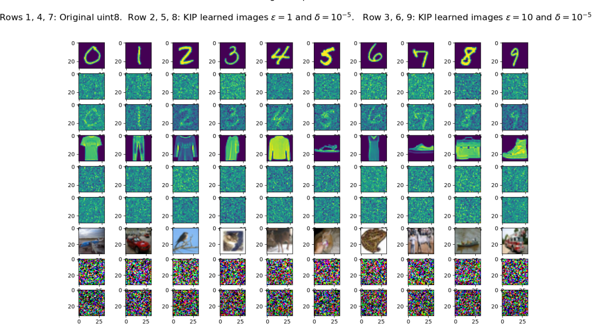
Figure 1: Image data comparison for MNIST, FASHION and CIFAR-10. The images plotted correspondo to real and distilled samples with DP-KIP for different $\epsilon$ values. Top row: MNIST original images. Second row: DP-KIP learned distilled images at $\epsilon=1$. Third row: DP-KIP learned distilled images at $\epsilon=10$. Fourth row: FashionMNIST original images. Fifth row: DP-KIP learned distilled images at $\epsilon=1$. Sixth row: DP-KIP learned distilled images at $\epsilon=10$. Seventh row: CIFAR10 original images. Eighth row: DP-KIP learned distilled images at $\epsilon=1$. Bottom row: DP-KIP learned distilled images at $\epsilon=10$.

5.1 Image data

We start by testing DP-KIP performance on MNIST (LeCun et al., 2010), FashionMNIST (Xiao et al., 2017), SVHN (Netzer et al., 2011), CIFAR-10 (Krizhevsky & Hinton, 2009) and CIFAR-100 datasets for image classification.

Each of MNIST and FashionMNIST datasets consists of 60,000 samples of $28\times 28$ grey scale images depicting handwritten digits and items of clothing, respectively, sorted into 10 classes. The SVHN dataset contains 600,000 samples of $32\times 32$ colour images of house numbers taken from Google Street View images, sorted into 10 classes. The CIFAR-10 dataset contains a 50,000-sample of $32\times 32$ colour images of 10 classes of objects, such as vehicles (cars and ships) and animals (horses and birds). CIFAR100 contains $100$ classes of objects.

In Table  1, we consider KIP as a non-private baseline and show as evaluation metric (for both private and non-private distilled samples) the averaged test accuracy using KRR as a classifier for 1, 10 and 50 distilled images per class over 5 independent runs. For DP-KIP we consider $\epsilon\in\{1,10\}$ and $\delta=10^{-5}$. The general trend is that creating more images per class improves the classification accuracy, while the gradient dimension in DP-SGD increases. In Fig. 1, we show the learned distilled images at $\epsilon=1$ and $\epsilon=10$. It is surprising that the images created at $\epsilon=10$ are not humanly discernible, while the classifiers can still achieve a good classification performance.

The detailed hyper-parameter setting can be found in Sec. A.1 in Appendix

Table 1: KRR test accuracy on Image datasets. The average over five independent runs.

	Imgs/	KIP FC	DP-KIP FC
	Class		$\epsilon=1$	$\epsilon=10$
MNIST	1	89.3 $\pm$ 0.1	82.7 $\pm$ 0.1	85.2 $\pm$ 0.1
	10	96.6 $\pm$ 0.1	87.5 $\pm$ 0.4	89.3 $\pm$ 0.3
	50	97.6 $\pm$ 0.1	92.7 $\pm$ 0.2	93.4 $\pm$ 0.1
FASHION	1	80.3 $\pm$ 0.4	76.9 $\pm$ 0.1	78.3 $\pm$ 0.1
	10	84.8 $\pm$ 0.4	77.7 $\pm$ 0.1	78.7 $\pm$ 0.4
	50	86.1 $\pm$ 0.1	78.8 $\pm$ 0.1	81.1 $\pm$ 0.1
SVHN	1	25.4 $\pm$ 0.3	24.9 $\pm$ 0.3	25.2 $\pm$ 0.2
	10	59.7 $\pm$ 0.5	40.5 $\pm$ 1.2	47.2 $\pm$ 0.6
	50	69.7 $\pm$ 0.1	52.7 $\pm$ 0.4	56.6 $\pm$ 0.4
CIFAR-10	1	39.3 $\pm$ 1.6	36.7 $\pm$ 0.3	37.3 $\pm$ 0.1
	10	49.1 $\pm$ 1.1	38.3 $\pm$ 0.3	39.7 $\pm$ 0.3
	50	52.1 $\pm$ 0.8	40.8 $\pm$ 0.2	43.7 $\pm$ 0.1
CIFAR-100	1	14.5 $\pm$ 0.4	9.9 $\pm$ 0.6	11.1 $\pm$ 0.1
	10	12.2 $\pm$ 0.2	10.1 $\pm$ 0.3	12.1 $\pm$ 0.4

In Table  2, we explore the performance of DP-KIP compared to other methods for private data generation (DP-CGAN, G-PATE, DataLens, GS-WGAN, DP-MERF, DP-Sinkhorn) and private gradient matching by Chen et al. (2022b). We report the test accuracy of a ConvNet downstream classifier consisting of 3 blocks, where each block contains one Conv layer with 128 filters, Instance Normalization, ReLU activation and AvgPooling modules and a FC layer as the final output. The classifier is trained using private data and then, it is tested on real test data over 3 independent runs for each method. Here, our method outperforms existing methods at the same privacy level.

Table 2: Left: Test accuracy of ConvNet downstream classifier trained on synthetic/distilled data with $\delta=10^{-5}$. Right: Test accuracy of ConvNet downstream classifier trained with fixed $\epsilon=10$ and $\delta=10^{-5}$ and varying the number of distilled samples per class. In concurrent work (Anonymous, 2023), the test accuracy on the same classifier tested on $50$ MNIST distilled samples created at $\epsilon=6.12$ and $\delta=10^{-5}$ is $97.35\%$; that on $50$ Fashion-MNIST distilled samples created at $\epsilon=6.72$ and $\delta=10^{-5}$ is $52.68\%$

	MNIST		FASHION
	$\epsilon=1$	$\epsilon=10$	$\epsilon=1$	$\epsilon=10$
DP-CGAN	-	52.5	-	50.2
G-PATE	58.8	80.9	58.1	69.3
DataLens	71.2	80.7	64.8	70.6
GS-WGAN	-	84.9	-	63.1
DP-MERF	72.7	85.7	61.2	72.4
DP-Sinkhorn	-	83.2	-	71.1
Chen et al. (2022a)
(20 Imgs/Class)	80.9	95.6	70.2	77.7
DP-KIP
(10 Imgs/Class)	93.53	95.39	87.7	89.1
DP-KIP
(20 Imgs/Class)	97.78	97.96	88.3	90.2

	MNIST			FASHION
Imgs/Class	10	20	full	10	20	full
Real	93.6	95.9	99.6	74.4	77.4	93.5
DPSGD	-	-	96.5	-	-	82.9
DP-CGAN	57.4	57.1	52.5	51.4	53.0	50.2
GS-WGAN	83.3	85.5	84.9	58.7	59.5	63.1
DP-MERF	80.2	83.2	85.7	66.6	67.9	72.4
Chen et al. (2022a)	94.9	95.6	-	75.6	77.7	-
DP-KIP	95.39	97.96	-	89.1	90.2	-

Table 3: Performance comparison on Tabular datasets. The average over five independent runs.

	Real		DP-CGAN		DP-GAN		DP-MERF		DP-HP		DP-KIP
			($1,10^{-5}$)-DP		($1,10^{-5}$)-DP		($1,10^{-5}$)-DP		($1,10^{-5}$)-DP		($1,10^{-5}$)-DP
adult	0.786	0.683	0.509	0.444	0.511	0.445	0.642	0.524	0.688	0.632	0.662	0.365
census	0.776	0.433	0.655	0.216	0.529	0.166	0.685	0.236	0.699	0.328	0.766	0.408
cervical	0.959	0.858	0.519	0.200	0.485	0.183	0.531	0.176	0.616	0.312	0.622	0.316
credit	0.924	0.864	0.664	0.356	0.435	0.150	0.751	0.622	0.786	0.744	0.892	0.610
epileptic	0.808	0.636	0.578	0.241	0.505	0.196	0.605	0.316	0.609	0.554	0.786	0.979
isolet	0.895	0.741	0.511	0.198	0.540	0.205	0.557	0.228	0.572	0.498	0.762	0.913
	F1		F1		F1		F1		F1		F1
covtype	0.820		0.285		0.492		0.467		0.537		0.582
intrusion	0.971		0.302		0.251		0.892		0.890		0.648

Table 4: Tabular datasets. Size, number of classes and feature types descriptions.

dataset	$\#$ samps	$\#$ classes	$\#$ features
isolet	4366	2	617 num
covtype	406698	7	10 num, 44 cat
epileptic	11500	2	178 num
credit	284807	2	29 num
cervical	753	2	11 num, 24 cat
census	199523	2	7 num, 33 cat
adult	48842	2	6 num, 8 cat
intrusion	394021	5	8 cat, 6 ord, 26 num

5.2 Tabular data

In the following we present DP-KIP results applied to eight different tabular datasets for imbalanced data. These datasets contain both numerical and categorical input features and are described in detail in Table  4. To evaluate the utility of the distilled samples, we train 12 commonly used classifiers on the distilled data samples and then evaluate their performance on real data for 5 independent runs.

For datasets with binary labels, we use the area under the receiver characteristics curve (ROC) and the area under the precision recall curve (PRC) as evaluation metrics, and for multi-class datasets, we use F1 score. Table  3 shows the average over the classifiers (averaged again over the 5 independent runs) trained on the synthetic privated generated samples for DP-CGAN(Torkzadehmahani et al., 2019), DP-GAN (Xie et al., 2018), DP-MERF(Harder et al., 2021) and DP-HP (Vinaroz et al., 2022) and trained on the privately distilled samples for DP-KIP under the same privacy budget $\epsilon=1$ and $\delta=10^{-5}$. Details on the classifiers used in evaluation can be found in Table  7.

For private synthetic methods we generate as many samples as the target dataset contains while for DP-KIP we set the images per class to 10. Unsurprisingly, our method outperforms the general data generation methods at the same privacy level.

6 Summary and Discussion

In this paper, we privatized KIP using DP-SGD and implemented this algorithm in JAX. Following KIP, our method uses infinite-dimensional features from a fully connected NTK. Experimental results show that our method ourperforms existing methods at the same privacy level.

Note that (Nguyen et al., 2021a, b) use an infinitely-wide convoluational network for NTK and further improves the performance. However, this code is not publicly available and when we contacted the authors, they were not able to share their code. We ended up implementing it ourselves. However, the KIP training with the convnet NTK requires an enormous memory (which only Googlers can fit in their memory in a distributed way) which we were unable to do at a decent size of mini-batch. Hence, in this paper, we only show the results of FC-NTK. In future work, we hope to further improve the performance using different NTK architectures including ConvNets.

Appendix A Expermental details

A.1 Image data

Here we provide the details of the DP-KIP training procedure we used on the image data experiments. Table  5 and Table  6 shows the number of epochs, batch size, learning rate, clipping norm $C$ and regularization parameter $\lambda$ used during training for each image classification dataset at the corresponding images per class distilled.

Table 5: DP-KIP hyper-parameter settings for Image data for $\epsilon=1$ and $\delta=10^{-5}$

	Imgs/Class	epochs	batch size	learning rate	$C$	$\lambda$
MNIST	1	10	500	$5\cdot 10^{-3}$	$10^{-2}$	$10^{-6}$
	10	10	500	$10^{-2}$	$10^{-6}$	$10^{-6}$
	50	10	500	$10^{-2}$	$10^{-6}$	$10^{-7}$
FASHION	1	10	500	$5\cdot 10^{-2}$	$10^{-6}$	$10^{-6}$
	10	10	500	0.1	$10^{-6}$	$10^{-5}$
	50	10	200	$10^{-2}$	$10^{-2}$	$10^{-6}$
SVHN	1	10	50	$10^{-1}$	$10^{-6}$	$10^{-6}$
	10	10	500	$5\cdot 10^{-2}$	$10^{-6}$	$10^{-6}$
	50	10	500	$10^{-2}$	$10^{-5}$	$10^{-2}$
CIFAR-10	1	20	200	$10^{-2}$	$10^{-4}$	$10^{-5}$
	10	10	500	$5\cdot 10^{-2}$	$10^{-5}$	$10^{-6}$
	50	10	500	$5\cdot 10^{-2}$	$10^{-3}$	$10^{-6}$
CIFAR-100	1	10	200	$10^{-2}$	$10^{-5}$	$10^{-7}$
	10	10	100	$10^{-2}$	$10^{-4}$	$10^{-7}$

Table 6: DP-KIP hyper-parameter settings for Image data for $\epsilon=10$ and $\delta=10^{-5}$

	Imgs/Class	epochs	batch size	learning rate	$C$	$\lambda$
MNIST	1	10	500	$5\cdot 10^{-3}$	$10^{-5}$	$10^{-6}$
	10	10	500	$5\cdot 10^{-3}$	$10^{-2}$	$10^{-6}$
	50	10	500	$5\cdot 10^{-3}$	$10^{-5}$	$10^{-6}$
FASHION	1	10	500	$10^{-2}$	$10^{-3}$	$10^{-6}$
	10	10	500	$10^{-2}$	$10^{-2}$	$10^{-5}$
	50	10	500	$10^{-2}$	$10^{-2}$	$10^{-7}$
SVHN	1	10	50	$5\cdot 10^{-2}$	$10^{-6}$	$10^{-6}$
	10	10	500	$10^{-1}$	$10^{-6}$	$10^{-6}$
	50	10	500	$10^{-2}$	$10^{-2}$	$10^{-7}$
CIFAR-10	1	10	500	$10^{-1}$	$10^{-6}$	$10^{-6}$
	10	10	500	$5\cdot 10^{-2}$	$10^{-5}$	$10^{-6}$
	50	10	500	$5\cdot 10^{-2}$	$10^{-5}$	$10^{-6}$
CIFAR-100	1	10	100	$10^{-2}$	$10^{-5}$	$10^{-6}$
	10	10	100	$10^{-2}$	$10^{-4}$	$10^{-6}$

A.2 Tabular data

Table 7: Hyperparameter settings for downstream classifiers used in tabular data experiments. Models are taken from scikit-learn 0.24.2 and xgboost 0.90 python packages and hyperparameters have been set to achieve reasonable accuracies while limiting runtimes. Paramters not listed are kept as default values.

Model	Parameters
Logistic Regression	solver: lbfgs, max_iter: 5000, multi_class: auto
Gaussian Naive Bayes	-
Bernoulli Naive Bayes	binarize: 0.5
LinearSVC	max_iter: 10000, tol: 1e-8, loss: hinge
Decision Tree	class_weight: balanced
LDA	solver: eigen, n_components: 9, tol: 1e-8, shrinkage: 0.5
Adaboost	n_estimators: 1000, learning_rate: 0.7, algorithm: SAMME.R
Bagging	max_samples: 0.1, n_estimators: 20
Random Forest	n_estimators: 100, class_weight: balanced
Gradient Boosting	subsample: 0.1, n_estimators: 50
MLP	-
XGB	colsample_bytree: 0.1, objective: multi:softprob, n_estimators: 50

Hyperparameters we used for Tabular data results can be found in our code repo.

References

- Abadi et al. (2016) Abadi, M., Chu, A., Goodfellow, I., McMahan, H. B., Mironov, I., Talwar, K., and Zhang, L. Deep learning with differential privacy. In Proceedings of the 2016 ACM SIGSAC Conference on Computer and Communications Security. ACM, oct 2016. doi: 10.1145/2976749.2978318. URL https://doi.org/10.1145%2F2976749.2978318.
- Anonymous (2023) Anonymous. Differentially private dataset condensation. In Submitted to The Eleventh International Conference on Learning Representations, 2023. URL https://openreview.net/forum?id=H8XpqEkbua_. under review.
- Arora et al. (2019) Arora, S., Du, S. S., Hu, W., Li, Z., Salakhutdinov, R., and Wang, R. On exact computation with an infinitely wide neural net. In Oh, A. H., Agarwal, A., Belgrave, D., and Cho, K. (eds.), Advances in Neural Information Processing Systems, 2019. URL https://openreview.net/pdf?id=rkl4aESeUH.
- Bradbury et al. (2018) Bradbury, J., Frostig, R., Hawkins, P., Johnson, M. J., Leary, C., Maclaurin, D., Necula, G., Paszke, A., VanderPlas, J., Wanderman-Milne, S., and Zhang, Q. JAX: composable transformations of Python+NumPy programs, 2018. URL http://github.com/google/jax.
- Cao et al. (2021) Cao, T., Bie, A., Vahdat, A., Fidler, S., and Kreis, K. Don’t generate me: Training differentially private generative models with sinkhorn divergence. In Ranzato, M., Beygelzimer, A., Dauphin, Y., Liang, P., and Vaughan, J. W. (eds.), Advances in Neural Information Processing Systems, volume 34, pp. 12480–12492. Curran Associates, Inc., 2021. URL https://proceedings.neurips.cc/paper/2021/file/67ed94744426295f96268f4ac1881b46-Paper.pdf.
- Carlini et al. (2022) Carlini, N., Feldman, V., and Nasr, M. No free lunch in ”privacy for free: How does dataset condensation help privacy”, 2022. URL https://arxiv.org/abs/2209.14987.
- Chen et al. (2020) Chen, D., Orekondy, T., and Fritz, M. GS-WGAN: A gradient-sanitized approach for learning differentially private generators. In Advances in Neural Information Processing Systems 33, 2020.
- Chen et al. (2022a) Chen, D., Kerkouche, R., and Fritz, M. Private set generation with discriminative information. In Oh, A. H., Agarwal, A., Belgrave, D., and Cho, K. (eds.), Advances in Neural Information Processing Systems, 2022a. URL https://openreview.net/forum?id=mxnxRw8jiru.
- Chen et al. (2022b) Chen, D., Kerkouche, R., and Fritz, M. Private set generation with discriminative information. In Neural Information Processing Systems (NeurIPS), 2022b.
- Dong et al. (2022a) Dong, T., Zhao, B., and Lyu, L. Privacy for free: How does dataset condensation help privacy? In Chaudhuri, K., Jegelka, S., Song, L., Szepesvari, C., Niu, G., and Sabato, S. (eds.), Proceedings of the 39th International Conference on Machine Learning, volume 162 of Proceedings of Machine Learning Research, pp. 5378–5396. PMLR, 17–23 Jul 2022a. URL https://proceedings.mlr.press/v162/dong22c.html.
- Dong et al. (2022b) Dong, X., Guo, J., Li, A., Ting, W.-T., Liu, C., and Kung, H. Neural mean discrepancy for efficient out-of-distribution detection. In Proceedings of the IEEE/CVF Conference on Computer Vision and Pattern Recognition (CVPR), pp. 19217–19227, June 2022b.
- Dwork & Roth (2014) Dwork, C. and Roth, A. The Algorithmic Foundations of Differential Privacy. Found. Trends Theor. Comput. Sci., 9:211–407, aug 2014. ISSN 1551-305X. doi: 10.1561/0400000042. URL http://dx.doi.org/10.1561/0400000042.
- Dwork et al. (2006a) Dwork, C., Kenthapadi, K., McSherry, F., Mironov, I., and Naor, M. Our data, ourselves: Privacy via distributed noise generation. In Eurocrypt, volume 4004, pp. 486–503. Springer, 2006a.
- Dwork et al. (2006b) Dwork, C., McSherry, F., Nissim, K., and Smith, A. Calibrating noise to sensitivity in private data analysis. In Halevi, S. and Rabin, T. (eds.), Theory of Cryptography, pp. 265–284, Berlin, Heidelberg, 2006b. Springer Berlin Heidelberg. ISBN 978-3-540-32732-5.
- Harder et al. (2021) Harder, F., Adamczewski, K., and Park, M. DP-MERF: Differentially private mean embeddings with randomfeatures for practical privacy-preserving data generation. In Banerjee, A. and Fukumizu, K. (eds.), Proceedings of The 24th International Conference on Artificial Intelligence and Statistics, volume 130 of Proceedings of Machine Learning Research, pp. 1819–1827. PMLR, 13–15 Apr 2021. URL http://proceedings.mlr.press/v130/harder21a.html.
- Jacot et al. (2018) Jacot, A., Gabriel, F., and Hongler, C. Neural tangent kernel: Convergence and generalization in neural networks. In Bengio, S., Wallach, H., Larochelle, H., Grauman, K., Cesa-Bianchi, N., and Garnett, R. (eds.), Advances in Neural Information Processing Systems, volume 31. Curran Associates, Inc., 2018. URL https://proceedings.neurips.cc/paper/2018/file/5a4be1fa34e62bb8a6ec6b91d2462f5a-Paper.pdf.
- Jia et al. (2021) Jia, S., Nezhadarya, E., Wu, Y., and Ba, J. Efficient statistical tests: A neural tangent kernel approach. In Meila, M. and Zhang, T. (eds.), Proceedings of the 38th International Conference on Machine Learning, volume 139 of Proceedings of Machine Learning Research, pp. 4893–4903. PMLR, 18–24 Jul 2021. URL https://proceedings.mlr.press/v139/jia21a.html.
- Krizhevsky & Hinton (2009) Krizhevsky, A. and Hinton, G. Learning multiple layers of features from tiny images. Technical Report 0, University of Toronto, Toronto, Ontario, 2009.
- LeCun et al. (2010) LeCun, Y., Cortes, C., and Burges, C. Mnist handwritten digit database. ATT Labs [Online]. Available: http://yann.lecun.com/exdb/mnist, 2, 2010.
- Lee et al. (2019) Lee, J., Xiao, L., Schoenholz, S., Bahri, Y., Novak, R., Sohl-Dickstein, J., and Pennington, J. Wide neural networks of any depth evolve as linear models under gradient descent. In Wallach, H., Larochelle, H., Beygelzimer, A., d'Alché-Buc, F., Fox, E., and Garnett, R. (eds.), Advances in Neural Information Processing Systems, volume 32. Curran Associates, Inc., 2019. URL https://proceedings.neurips.cc/paper/2019/file/0d1a9651497a38d8b1c3871c84528bd4-Paper.pdf.
- Lee et al. (2020) Lee, J., Schoenholz, S., Pennington, J., Adlam, B., Xiao, L., Novak, R., and Sohl-Dickstein, J. Finite versus infinite neural networks: an empirical study. In Larochelle, H., Ranzato, M., Hadsell, R., Balcan, M., and Lin, H. (eds.), Advances in Neural Information Processing Systems, volume 33, pp. 15156–15172. Curran Associates, Inc., 2020. URL https://proceedings.neurips.cc/paper/2020/file/ad086f59924fffe0773f8d0ca22ea712-Paper.pdf.
- Long et al. (2021) Long, Y., Wang, B., Yang, Z., Kailkhura, B., Zhang, A., Gunter, C., and Li, B. G-PATE: Scalable differentially private data generator via private aggregation of teacher discriminators. In Ranzato, M., Beygelzimer, A., Dauphin, Y., Liang, P., and Vaughan, J. W. (eds.), Advances in Neural Information Processing Systems, volume 34, pp. 2965–2977. Curran Associates, Inc., 2021. URL https://proceedings.neurips.cc/paper/2021/file/171ae1bbb81475eb96287dd78565b38b-Paper.pdf.
- Netzer et al. (2011) Netzer, Y., Wang, T., Coates, A., Bissacco, A., Wu, B., and Ng, A. Y. Reading digits in natural images with unsupervised feature learning. In NIPS Workshop on Deep Learning and Unsupervised Feature Learning 2011, 2011. URL http://ufldl.stanford.edu/housenumbers/nips2011_housenumbers.pdf.
- Nguyen et al. (2021a) Nguyen, T., Chen, Z., and Lee, J. Dataset meta-learning from kernel ridge-regression. In International Conference on Learning Representations, 2021a. URL https://openreview.net/forum?id=l-PrrQrK0QR.
- Nguyen et al. (2021b) Nguyen, T., Novak, R., Xiao, L., and Lee, J. Dataset distillation with infinitely wide convolutional networks. In Ranzato, M., Beygelzimer, A., Dauphin, Y., Liang, P., and Vaughan, J. W. (eds.), Advances in Neural Information Processing Systems, volume 34, pp. 5186–5198. Curran Associates, Inc., 2021b. URL https://proceedings.neurips.cc/paper/2021/file/299a23a2291e2126b91d54f3601ec162-Paper.pdf.
- Novak et al. (2020) Novak, R., Xiao, L., Hron, J., Lee, J., Alemi, A. A., Sohl-Dickstein, J., and Schoenholz, S. S. Neural tangents: Fast and easy infinite neural networks in python. In International Conference on Learning Representations, 2020. URL https://github.com/google/neural-tangents.
- Torkzadehmahani et al. (2019) Torkzadehmahani, R., Kairouz, P., and Paten, B. DP-CGAN: Differentially private synthetic data and label generation. In The IEEE Conference on Computer Vision and Pattern Recognition (CVPR) Workshops, June 2019.
- Vinaroz et al. (2022) Vinaroz, M., Charusaie, M.-A., Harder, F., Adamczewski, K., and Park, M. J. Hermite polynomial features for private data generation. In Chaudhuri, K., Jegelka, S., Song, L., Szepesvari, C., Niu, G., and Sabato, S. (eds.), Proceedings of the 39th International Conference on Machine Learning, volume 162 of Proceedings of Machine Learning Research, pp. 22300–22324. PMLR, 17–23 Jul 2022. URL https://proceedings.mlr.press/v162/vinaroz22a.html.
- Wang et al. (2021) Wang, B., Wu, F., Long, Y., Rimanic, L., Zhang, C., and Li, B. Datalens: Scalable privacy preserving training via gradient compression and aggregation. In Proceedings of the 2021 ACM SIGSAC Conference on Computer and Communications Security, CCS ’21, pp. 2146–2168, New York, NY, USA, 2021. Association for Computing Machinery. ISBN 9781450384544. doi: 10.1145/3460120.3484579. URL https://doi.org/10.1145/3460120.3484579.
- Wang et al. (2018) Wang, T., Zhu, J., Torralba, A., and Efros, A. A. Dataset distillation. CoRR, abs/1811.10959, 2018. URL http://arxiv.org/abs/1811.10959.
- Wang et al. (2019) Wang, Y.-X., Balle, B., and Kasiviswanathan, S. P. Subsampled rényi differential privacy and analytical moments accountant. volume 89 of Proceedings of Machine Learning Research, pp. 1226–1235. PMLR, April 2019.
- Xiao et al. (2017) Xiao, H., Rasul, K., and Vollgraf, R. Fashion-mnist: a novel image dataset for benchmarking machine learning algorithms. arXiv preprint arXiv:1708.07747, 2017.
- Xie et al. (2018) Xie, L., Lin, K., Wang, S., Wang, F., and Zhou, J. Differentially private generative adversarial network. CoRR, abs/1802.06739, 2018.
- Zhao et al. (2021) Zhao, B., Mopuri, K. R., and Bilen, H. Dataset condensation with gradient matching. In International Conference on Learning Representations, 2021. URL https://openreview.net/forum?id=mSAKhLYLSsl.