Abstract

Robustness and safety are critical for the trustworthy deployment of deep reinforcement learning in real-world decision making applications. In particular, we require algorithms that can guarantee robust, safe performance in the presence of general environment disturbances, while making limited assumptions on the data collection process during training. In this work, we propose a safe reinforcement learning framework with robustness guarantees through the use of an optimal transport cost uncertainty set. We provide an efficient, theoretically supported implementation based on Optimal Transport Perturbations, which can be applied in a completely offline fashion using only data collected in a nominal training environment. We demonstrate the robust, safe performance of our approach on a variety of continuous control tasks with safety constraints in the Real-World Reinforcement Learning Suite.

1 Introduction

Deep reinforcement learning (RL) is a data-driven framework for sequential decision making that has demonstrated the ability to solve complex tasks, making it a promising approach for improving real-world decision making. In order for deep RL to be trusted for deployment in real-world decision making settings, however, robustness and safety are of the utmost importance (Xu et al., 2022). As a result, techniques have been developed to incorporate both robustness and safety into deep RL. Robust RL methods protect against worst-case environment transitions, while safe RL methods incorporate safety constraints into the training process.

In real-world applications, disturbances in the environment can take many forms that are difficult to model in advance. Therefore, we require methods that can guarantee robust and safe performance under general forms of environment uncertainty. Unfortunately, popular approaches to robustness in deep RL consider very structured forms of uncertainty in order to facilitate efficient implementations. Adversarial methods implement a specific type of perturbation, such as the application of a physical force (Pinto et al., 2017) or a change in the action that is deployed (Tessler et al., 2019a). Parametric approaches, on the other hand, consider robustness with respect to environment characteristics that can be altered in a simulator (Rajeswaran et al., 2017; Peng et al., 2018; Mankowitz et al., 2020). When we lack domain knowledge on the structure of potential disturbances, these techniques may not guarantee robustness and safety.

Another drawback of existing approaches is their need to directly modify the environment during training. Parametric methods assume the ability to generate a range of training environments with a detailed simulator, while adversarial methods directly influence the data collection process by attempting to negatively impact performance. In applications where simulators are inaccurate or unavailable, however, parametric methods cannot be applied and real-world data collection may be required for training. In this context, it is also undesirable to implement adversarial perturbations while interacting in the environment. Therefore, in many real-world domains, we must consider alternative methods for learning safe policies with robustness guarantees.

In this work, we propose a safe RL framework that provides robustness to general forms of environment disturbances using standard data collection in a nominal training environment. We consider robustness over a general uncertainty set defined using the optimal transport cost between environment transitions, and we leverage optimal transport theory to demonstrate how our framework can be efficiently implemented by applying Optimal Transport Perturbations to state transitions in a completely offline fashion. These perturbations can be added to the training process of any safe RL algorithm to incorporate robustness to unknown disturbances, without harming performance during training or requiring access to a range of simulated training environments.

We summarize our contributions as follows:

1. We formulate a safe RL framework that incorporates robustness to general disturbances using the optimal transport cost between environment transitions.

2. We show that the resulting distributionally robust optimization problems over transition distributions can be reformulated as constrained adversarial perturbations to state transitions in the training environment.

3. We propose an efficient deep RL implementation of our Optimal Transport Perturbations, which can be applied in a completely offline fashion without impacting data collection during training.

4. We demonstrate that the use of Optimal Transport Perturbations leads to robust and safe performance both during training and in the presence of disturbances through experiments on continuous control tasks with safety constraints in the Real-World RL Suite (Dulac-Arnold et al., 2020; 2021).

2 Related Work

2.1 Safe Reinforcement Learning

The most common approach to modeling safety in RL is to incorporate constraints on expected total costs (Altman, 1999). In recent years, several deep RL algorithms have been developed for this framework. A popular approach is to solve the Lagrangian relaxation of the constrained problem (Tessler et al., 2019b; Ray et al., 2019; Stooke et al., 2020), which is supported by theoretical results that constrained RL has zero duality gap (Paternain et al., 2019). Xu et al. (2021), on the other hand, consider immediate switching between the reward and cost objectives to better satisfy safety during training. Alternatively, Achiam et al. (2017) and Liu et al. (2022) construct closed-form solutions to guide policy updates in safe RL.

A related line of work focuses on the issue of safe exploration during data collection. In order to promote safety throughout trajectory rollouts, these methods correct potentially dangerous actions through the use of control barrier functions (Cheng et al., 2019; Emam et al., 2021; Ma et al., 2021), safety layers (Dalal et al., 2018), learned safety critics (Srinivasan et al., 2020; Bharadhwaj et al., 2021), and recovery policies (Thananjeyan et al., 2021; Wagener et al., 2021). In particular, Bharadhwaj et al. (2021) learn a conservative estimate of the safety critic in order to protect against safety violations during training. Our robust perspective towards safety can be viewed as an alternative method for learning a conservative safety critic, which guarantees safety both during and after training by guarding against unknown environment disturbances.

2.2 Robust Reinforcement Learning

Robust RL methods account for uncertainty in the environment by considering worst-case transition distributions from an uncertainty set (Nilim & Ghaoui, 2005; Iyengar, 2005). In order to scale the robust RL framework to the deep RL setting, most techniques have focused on parametric uncertainty or adversarial training.

Domain randomization (Tobin et al., 2017; Peng et al., 2018) represents a popular approach to parametric uncertainty in sim-to-real transfer settings, where a policy is trained to maximize average performance across a range of simulated training environments. These environments are generated by modifying important parameters in the simulator, which are often determined based on domain knowledge. The goal of maximizing average performance over a range of training environments has also been referred to as a soft-robust approach (Derman et al., 2018). Other methods directly impose a robust perspective towards parametric uncertainty by focusing on the worst-case training environments generated over a range of simulator parameters (Rajeswaran et al., 2017; Abdullah et al., 2019; Mankowitz et al., 2020). All of these approaches assume access to a simulated version of the real environment, as well as the ability to modify parameters of this simulator.

Adversarial RL methods represent an alternative approach to robustness that introduce perturbations directly into the training process. In order to learn policies that perform well under worst-case disturbances, these perturbations are trained to minimize performance. Deep RL approaches to adversarial training have introduced perturbations in the form of physical forces in the environment (Pinto et al., 2017), as well as adversarial corruptions to actions (Tessler et al., 2019a; Vinitsky et al., 2020) and state observations (Mandlekar et al., 2017; Zhang et al., 2020; Kuang et al., 2022). In this work, we learn adversarial perturbations on state transitions, but different from adversarial RL methods we apply these perturbations in a completely offline fashion without impacting the data collection process.

Finally, safety and robustness have recently been considered together in a unified RL framework. Mankowitz et al. (2021) and Russel et al. (2021) propose a formulation that incorporates robustness into both the objective and constraints in safe RL. We consider this general framework as a starting point for our work.

3 Preliminaries

3.1 Safe Reinforcement Learning

Consider an infinite-horizon, discounted Constrained Markov Decision Process (C-MDP) (Altman, 1999) defined by the tuple $(\mathcal{S},\mathcal{A},p,r,c,\rho_{0},\gamma)$, where $\mathcal{S}$ is the set of states, $\mathcal{A}$ is the set of actions, $p:\mathcal{S}\times\mathcal{A}\rightarrow P(\mathcal{S})$ is the transition probability function where $P(\mathcal{S})$ denotes the space of probability measures over $\mathcal{S}$, $r:\mathcal{S}\times\mathcal{A}\rightarrow\mathbb{R}$ is the reward function, $c:\mathcal{S}\times\mathcal{A}\rightarrow\mathbb{R}$ is the cost function, $\rho_{0}$ is the initial state distribution, and $\gamma$ is the discount rate.

We model the agent’s decisions as a stationary policy $\pi:\mathcal{S}\rightarrow P(\mathcal{A})$. For a given C-MDP and policy $\pi$, the expected total discounted rewards and costs are given by $J_{p,r}(\pi)=\mathop{\mathbb{E}}_{\tau\sim(\pi,p)}\left[\sum_{t=0}^{\infty}\gamma^{t}r(s_{t},a_{t})\right]$ and $J_{p,c}(\pi)=\mathop{\mathbb{E}}_{\tau\sim(\pi,p)}\left[\sum_{t=0}^{\infty}\gamma^{t}c(s_{t},a_{t})\right]$, respectively, where $\tau\sim(\pi,p)$ represents a trajectory sampled according to $s_{0}\sim\rho_{0}$, $a_{t}\sim\pi(\,\cdot\mid s_{t})$, and $s_{t+1}\sim p(\,\cdot\mid s_{t},a_{t})$. The goal of safe RL is to find a policy $\pi$ that maximizes the constrained optimization problem

$$\begin{split}\max_{\pi}\quad&J_{p,r}(\pi)\\ \textnormal{s.t.}\quad&J_{p,c}(\pi)\leq B,\end{split}$$ (1)

where $B$ is a safety budget on expected total discounted costs.

We denote the state-action value functions (i.e., Q functions) of $\pi$ for a given C-MDP as $Q^{\pi}_{p,r}(s,a)$ and $Q^{\pi}_{p,c}(s,a)$, and the state value functions as $V^{\pi}_{p,r}(s)=\mathop{\mathbb{E}}_{a\sim\pi(\cdot\mid s)}[Q^{\pi}_{p,r}(s,a)]$ and $V^{\pi}_{p,c}(s)=\mathop{\mathbb{E}}_{a\sim\pi(\cdot\mid s)}[Q^{\pi}_{p,c}(s,a)]$. Policy optimization techniques (Xu et al., 2021; Liu et al., 2022) iteratively optimize (1) by considering the related optimization problem

$$\begin{split}\max_{\pi}\quad&\mathop{\mathbb{E}}_{s\sim\mathcal{D}}\left[\mathop{\mathbb{E}}_{a\sim\pi(\cdot\mid s)}\left[Q^{\pi_{k}}_{p,r}(s,a)\right]\right]\\ \textnormal{s.t.}\quad&\mathop{\mathbb{E}}_{s\sim\mathcal{D}}\left[\mathop{\mathbb{E}}_{a\sim\pi(\cdot\mid s)}\left[Q^{\pi_{k}}_{p,c}(s,a)\right]\right]\leq B,\end{split}$$ (2)

where $\pi_{k}$ is the current policy and $\mathcal{D}$ represents data collected during training.

3.2 Robust and Safe Reinforcement Learning

We are often interested in finding a policy $\pi$ that achieves strong, safe performance across a range of related environments. In order to accomplish this, Mankowitz et al. (2021) and Russel et al. (2021) propose a Robust Constrained MDP (RC-MDP) framework defined by the tuple $(\mathcal{S},\mathcal{A},\mathcal{P},r,c,\rho_{0},\gamma)$, where $\mathcal{P}$ represents an uncertainty set of transition models. We assume $\mathcal{P}$ takes the form $\mathcal{P}=\bigotimes_{(s,a)\in\mathcal{S}\times\mathcal{A}}\mathcal{P}_{s,a}$, where $\mathcal{P}_{s,a}$ is a set of transition models $p_{s,a}=p(\,\cdot\mid s,a)\in P(\mathcal{S})$ at a given state-action pair and $\mathcal{P}$ is the product of these sets. This structure is referred to as rectangularity, and is a common assumption in the literature (Nilim & Ghaoui, 2005; Iyengar, 2005).

The RC-MDP framework leads to a robust version of (1) given by

$$\begin{split}\max_{\pi}\quad&\inf_{p\in\mathcal{P}}J_{p,r}(\pi)\\ \textnormal{s.t.}\quad&\sup_{p\in\mathcal{P}}J_{p,c}(\pi)\leq B.\end{split}$$ (3)

As in the standard safe RL setting, we can iteratively optimize (3) by considering the related optimization problem

$$\begin{split}\max_{\pi}\quad&\mathop{\mathbb{E}}_{s\sim\mathcal{D}}\left[\mathop{\mathbb{E}}_{a\sim\pi(\cdot\mid s)}\left[Q^{\pi_{k}}_{\mathcal{P},r}(s,a)\right]\right]\\ \textnormal{s.t.}\quad&\mathop{\mathbb{E}}_{s\sim\mathcal{D}}\left[\mathop{\mathbb{E}}_{a\sim\pi(\cdot\mid s)}\left[Q^{\pi_{k}}_{\mathcal{P},c}(s,a)\right]\right]\leq B,\end{split}$$ (4)

where $Q^{\pi}_{\mathcal{P},r}(s,a)$ and $Q^{\pi}_{\mathcal{P},c}(s,a)$ represent robust Q functions. Alternatively, if we only care about robustness with respect to safety, we can instead consider a nominal or optimistic objective in (4) to promote exploration.

4 Optimal Transport Uncertainty Set

Compared to the standard safe RL update in (2), the only difference in the robust and safe RL update of (4) comes from the use of robust Q functions. Therefore, in order to incorporate robustness into existing deep safe RL algorithms, we must be able to efficiently learn $Q^{\pi}_{\mathcal{P},r}(s,a)$ and $Q^{\pi}_{\mathcal{P},c}(s,a)$. We can write these robust Q functions recursively as

$$Q^{\pi}_{\mathcal{P},r}(s,a) =r(s,a)+\gamma\inf_{p_{s,a}\in\mathcal{P}_{s,a}}\mathop{\mathbb{E}}_{s^{\prime}\sim p_{s,a}}\left[V^{\pi}_{\mathcal{P},r}(s^{\prime})\right],$$

$$Q^{\pi}_{\mathcal{P},c}(s,a) =c(s,a)+\gamma\sup_{p_{s,a}\in\mathcal{P}_{s,a}}\mathop{\mathbb{E}}_{s^{\prime}\sim p_{s,a}}\left[V^{\pi}_{\mathcal{P},c}(s^{\prime})\right],$$

where we define the corresponding robust state value functions as $V^{\pi}_{\mathcal{P},r}(s^{\prime})=\mathop{\mathbb{E}}_{a^{\prime}\sim\pi(\cdot\mid s^{\prime})}\left[Q^{\pi}_{\mathcal{P},r}(s^{\prime},a^{\prime})\right]$ and $V^{\pi}_{\mathcal{P},c}(s^{\prime})=\mathop{\mathbb{E}}_{a^{\prime}\sim\pi(\cdot\mid s^{\prime})}\left[Q^{\pi}_{\mathcal{P},c}(s^{\prime},a^{\prime})\right]$. The corresponding robust Bellman operators (Nilim & Ghaoui, 2005; Iyengar, 2005) can be written as

$$\mathcal{T}^{\pi}_{\mathcal{P},r}Q_{r}(s,a) :=r(s,a)+\gamma\inf_{p_{s,a}\in\mathcal{P}_{s,a}}\mathop{\mathbb{E}}_{s^{\prime}\sim p_{s,a}}\left[V_{r}^{\pi}(s^{\prime})\right],$$ (5)

$$\mathcal{T}^{\pi}_{\mathcal{P},c}Q_{c}(s,a) :=c(s,a)+\gamma\sup_{p_{s,a}\in\mathcal{P}_{s,a}}\mathop{\mathbb{E}}_{s^{\prime}\sim p_{s,a}}\left[V_{c}^{\pi}(s^{\prime})\right],$$ (6)

where we write $V_{r}^{\pi}(s^{\prime})=\mathop{\mathbb{E}}_{a^{\prime}\sim\pi(\cdot\mid s^{\prime})}\left[Q_{r}(s^{\prime},a^{\prime})\right]$ and $V_{c}^{\pi}(s^{\prime})=\mathop{\mathbb{E}}_{a^{\prime}\sim\pi(\cdot\mid s^{\prime})}\left[Q_{c}(s^{\prime},a^{\prime})\right]$.

Note that $\mathcal{T}^{\pi}_{\mathcal{P},r}$ and $\mathcal{T}^{\pi}_{\mathcal{P},c}$ are contraction operators, with $Q^{\pi}_{\mathcal{P},r}(s,a)$ and $Q^{\pi}_{\mathcal{P},c}(s,a)$ their respective unique fixed points (Nilim & Ghaoui, 2005; Iyengar, 2005). Because $\mathcal{T}^{\pi}_{\mathcal{P},r}$ and $\mathcal{T}^{\pi}_{\mathcal{P},c}$ are contraction operators, we can apply standard temporal difference (TD) learning techniques to learn these robust Q functions. In order to do so, we must be able to calculate the Bellman targets in (5) and (6), which involve optimization problems over transition distributions that depend on the choice of uncertainty set $\mathcal{P}_{s,a}$ at every state-action pair. Popular choices of $\mathcal{P}_{s,a}$ in the literature require the ability to change physical parameters of the environment (Peng et al., 2018) or directly apply adversarial perturbations during trajectory rollouts (Tessler et al., 2019a) to calculate worst-case transitions.

In this work, we use optimal transport theory to consider an uncertainty set that can be efficiently implemented in a model-free fashion using only samples collected from a nominal environment. In order to do so, we assume that $\mathcal{S}$ is a Polish space (i.e., a separable, completely metrizable topological space). Note that the Euclidean space $\mathbb{R}^{n}$ is Polish, so this is not very restrictive. Next, we define $\mathcal{P}_{s,a}$ using the optimal transport cost between transition distributions.

Definition 4.1 (Optimal Transport Cost).

Let $\mathcal{S}$ be a Polish space, and let $d:\mathcal{S}\times\mathcal{S}\rightarrow\mathbb{R}_{+}$ be a non-negative, lower semicontinuous function satisfying $d(s^{\prime},s^{\prime})=0$ for all $s^{\prime}\in\mathcal{S}$. Then, the optimal transport cost between two transition distributions $\hat{p}_{s,a},p_{s,a}\in P(\mathcal{S})$ is defined as

$$\textnormal{OTC}_{d}(\hat{p}_{s,a},p_{s,a})=\inf_{\nu\in\Gamma\left(\hat{p}_{s,a},p_{s,a}\right)}\int_{\mathcal{S}\times\mathcal{S}}d(\hat{s}^{\prime},s^{\prime})\textnormal{d}\nu(\hat{s}^{\prime},s^{\prime}),$$

where $\Gamma(\hat{p}_{s,a},p_{s,a})$ is the set of all couplings of $\hat{p}_{s,a}$ and $p_{s,a}$.

If $d$ is chosen to be a metric raised to some power $p\geq 1$, we recover the $p$-Wasserstein distance raised to the power $p$ as a special case. If we let $d(\hat{s}^{\prime},s^{\prime})=\mathbf{1}_{\hat{s}^{\prime}\neq s^{\prime}}$, we recover the total variation distance as a special case (Villani, 2008).

By considering the optimal transport cost from some nominal transition distribution $\hat{p}_{s,a}$, we define the optimal transport uncertainty set as follows.

Definition 4.2 (Optimal Transport Uncertainty Set).

For a given nominal transition distribution $\hat{p}_{s,a}$ and radius $\epsilon_{s,a}$ at state-action pair $(s,a)\in\mathcal{S}\times\mathcal{A}$, the optimal transport uncertainty set is defined as

$$\mathcal{P}_{s,a}=\left\{p_{s,a}\in P(\mathcal{S})\mid\textnormal{OTC}_{d}(\hat{p}_{s,a},p_{s,a})\leq\epsilon_{s,a}\right\}.$$

This uncertainty set has previously been considered in robust RL for the special case of the Wasserstein distance (Abdullah et al., 2019; Hou et al., 2020; Kuang et al., 2022).

The use of optimal transport cost to compare transition distributions has several benefits. First, optimal transport cost accounts for the relationship between states in $\mathcal{S}$ through the function $d$, and we can choose $d$ to reflect the geometry of $\mathcal{S}$ in a meaningful way. In particular, optimal transport cost allows significant flexibility in the choice of $d$, including threshold-based binary comparisons between states that are not metrics or pseudo-metrics (Pydi & Jog, 2020). Next, optimal transport cost remains valid for distributions that do not share the same support, unlike other popular measures between distributions such as the Kullback-Leibler divergence. In particular, the optimal transport uncertainty set can be applied to both stochastic and deterministic transitions. Finally, as we will show in the following sections, the use of an optimal transport uncertainty set results in an efficient model-free implementation of robust and safe RL that only requires the ability to collect data in a nominal environment.

5 Reformulation as Adversarial Perturbations to State Transitions

In order to provide tractable reformulations of the Bellman operators in (5) and (6), we consider the following main assumptions.

Assumption 5.1.

For any $\pi$ and $Q_{r}(s^{\prime},a^{\prime})$ in (5), $V_{r}^{\pi}(s^{\prime})=\mathop{\mathbb{E}}_{a^{\prime}\sim\pi(\cdot\mid s^{\prime})}\left[Q_{r}(s^{\prime},a^{\prime})\right]$ is lower semicontinuous and $\mathbb{E}_{s^{\prime}\sim\hat{p}_{s,a}}|V_{r}^{\pi}(s^{\prime})|<\infty$. For any $\pi$ and $Q_{c}(s^{\prime},a^{\prime})$ in (6), $V_{c}^{\pi}(s^{\prime})=\mathop{\mathbb{E}}_{a^{\prime}\sim\pi(\cdot\mid s^{\prime})}\left[Q_{c}(s^{\prime},a^{\prime})\right]$ is upper semicontinuous and $\mathbb{E}_{s^{\prime}\sim\hat{p}_{s,a}}|V_{c}^{\pi}(s^{\prime})|<\infty$.

Assumption 5.2.

Optimal transport plans exist for the distributionally robust optimization problems in (5) and (6).

Note that Assumptions 5.1–5.2 correspond to assumptions in Blanchet & Murthy (2019) applied to our setting. In practice, the use of neural network representations results in continuous value functions, which are bounded for the common case when rewards and costs are bounded, respectively. A sufficient condition for Assumption 5.2 to hold is if $\mathcal{S}$ is compact, or if we restrict our attention to a compact subset of next states in our definition of $\mathcal{P}_{s,a}$ which is reasonable in practice. Blanchet & Murthy (2019) also provide other sufficient conditions for Assumption 5.2 to hold.

Under these assumptions, we can reformulate the Bellman operators in (5) and (6) to allow for efficient deep RL implementations.

Lemma 5.3.

Let Assumption 5.1 hold. Then, we have

$$\mathcal{T}^{\pi}_{\mathcal{P},r}Q_{r}(s,a)=r(s,a)+\gamma\,\,\sup_{\lambda\geq 0}\,\,\left\{\vphantom{\mathop{\mathbb{E}}_{\hat{s}^{\prime}\sim\hat{p}_{s,a}}\left[\,\,\inf_{s^{\prime}\in\mathcal{S}}\,\,V_{r}^{\pi}(s^{\prime})+\lambda\left(d(\hat{s}^{\prime},s^{\prime})-\epsilon_{s,a}\right)\right]}\right.$$

$$\left.\quad\mathop{\mathbb{E}}_{\hat{s}^{\prime}\sim\hat{p}_{s,a}}\left[\,\,\inf_{s^{\prime}\in\mathcal{S}}\,\,V_{r}^{\pi}(s^{\prime})+\lambda\left(d(\hat{s}^{\prime},s^{\prime})-\epsilon_{s,a}\right)\right]\right\},$$ (7)

$$\mathcal{T}^{\pi}_{\mathcal{P},c}Q_{c}(s,a)=c(s,a)+\gamma\,\,\inf_{\lambda\geq 0}\,\,\left\{\vphantom{\mathop{\mathbb{E}}_{\hat{s}^{\prime}\sim\hat{p}_{s,a}}\left[\,\,\sup_{s^{\prime}\in\mathcal{S}}\,\,V_{c}^{\pi}(s^{\prime})-\lambda\left(d(\hat{s}^{\prime},s^{\prime})-\epsilon_{s,a}\right)\right]}\right.$$

$$\left.\quad\mathop{\mathbb{E}}_{\hat{s}^{\prime}\sim\hat{p}_{s,a}}\left[\,\,\sup_{s^{\prime}\in\mathcal{S}}\,\,V_{c}^{\pi}(s^{\prime})-\lambda\left(d(\hat{s}^{\prime},s^{\prime})-\epsilon_{s,a}\right)\right]\right\}.$$ (8)

Proof.

According to Theorem 1 in Blanchet & Murthy (2019), optimal transport strong duality holds for the distributionally robust optimization problems in (5) and (6) under Assumption 5.1. By applying optimal transport strong duality and substituting these results into (5) and (6), we arrive at the results in (7) and (8), respectively. See the Appendix for details. ∎

With the addition of Assumption 5.2, we can further reformulate the results in Lemma 5.3 to arrive at a tractable result that can be efficiently implemented in a deep RL setting.

Theorem 5.4.

Let Assumptions 5.1–5.2 hold, and let $\mathcal{G}$ be the set of all functions from $\mathcal{S}$ to $\mathcal{S}$. Then, we have

$$\mathcal{T}^{\pi}_{\mathcal{P},r}Q_{r}(s,a) =r(s,a)+\gamma\mathop{\mathbb{E}}_{\hat{s}^{\prime}\sim\hat{p}_{s,a}}\left[V_{r}^{\pi}(g^{r}_{s,a}(\hat{s}^{\prime}))\right],$$ (9)

$$\mathcal{T}^{\pi}_{\mathcal{P},c}Q_{c}(s,a) =c(s,a)+\gamma\mathop{\mathbb{E}}_{\hat{s}^{\prime}\sim\hat{p}_{s,a}}\left[V_{c}^{\pi}(g^{c}_{s,a}(\hat{s}^{\prime}))\right],$$ (10)

where $g^{r}_{s,a}:\mathcal{S}\rightarrow\mathcal{S}$ is a minimizer of

$$\begin{split}\min_{g\in\mathcal{G}}\quad&\mathop{\mathbb{E}}_{\hat{s}^{\prime}\sim\hat{p}_{s,a}}\left[V_{r}^{\pi}(g(\hat{s}^{\prime}))\right]\\ \textnormal{s.t.}\quad&\mathop{\mathbb{E}}_{\hat{s}^{\prime}\sim\hat{p}_{s,a}}\left[d(\hat{s}^{\prime},g(\hat{s}^{\prime}))\right]\leq\epsilon_{s,a},\end{split}$$ (11)

and $g^{c}_{s,a}:\mathcal{S}\rightarrow\mathcal{S}$ is a maximizer of

$$\begin{split}\max_{g\in\mathcal{G}}\quad&\mathop{\mathbb{E}}_{\hat{s}^{\prime}\sim\hat{p}_{s,a}}\left[V_{c}^{\pi}(g(\hat{s}^{\prime}))\right]\\ \textnormal{s.t.}\quad&\mathop{\mathbb{E}}_{\hat{s}^{\prime}\sim\hat{p}_{s,a}}\left[d(\hat{s}^{\prime},g(\hat{s}^{\prime}))\right]\leq\epsilon_{s,a},\end{split}$$ (12)

for a given state-action pair $(s,a)\in\mathcal{S}\times\mathcal{A}$.

Proof.

First, we show that the dual problems to (11) and (12) appear in the right-hand side of (7) and (8), repectively. Next, we use Assumption 5.2 to show that strong duality holds for these pairs of primal-dual problems. See the Appendix for details. ∎

Theorem 5.4 demonstrates that we can calculate the Bellman operators $\mathcal{T}^{\pi}_{\mathcal{P},r}$ and $\mathcal{T}^{\pi}_{\mathcal{P},c}$ by using samples collected from a nominal environment with transition distributions $\hat{p}_{s,a}$, and adversarially perturbing the next state samples according to (11) and (12), respectively. We refer to the resulting changes in state transitions as Optimal Transport Perturbations (OTP). As a result, we have replaced difficult optimization problems over distribution space in (5) and (6) with the tractable problems of computing Optimal Transport Perturbations in state space. Theorem 5.4 represents the main theoretical contribution of our work, which directly motivates an efficient deep RL implementation of robust and safe RL.

Finally, note that these perturbed state transitions are only used to calculate the Bellman targets in (9) and (10) for training the robust Q functions $Q^{\pi}_{\mathcal{P},r}(s,a)$ and $Q^{\pi}_{\mathcal{P},c}(s,a)$. Therefore, unlike other adversarial approaches to robust RL (Pinto et al., 2017; Tessler et al., 2019a; Vinitsky et al., 2020), we do not need to apply our Optimal Transport Perturbations during trajectory rollouts. Instead, these perturbations are applied in a completely offline fashion. See Figure 1 for an illustration.

Figure 1: Illustration of Optimal Transport Perturbations from Theorem 5.4 for a given next state sample $\hat{s}^{\prime}\sim\hat{p}_{s,a}$ in the nominal environment. The black arrow denotes the state transition observed in the nominal environment, and the shaded area denotes the feasible set in $\mathcal{S}$ from (11) and (12). Theorem 5.4 calculates separate next state perturbations for the robust reward Bellman operator (shown in blue) and the robust cost Bellman operator (shown in orange). The dashed arrows denote imagined transitions used only to calculate Bellman operators.

6 Perturbation Networks for Deep Reinforcement Learning

From Theorem 5.4, we can calculate Bellman targets for our robust Q functions $Q^{\pi}_{\mathcal{P},r}(s,a)$ and $Q^{\pi}_{\mathcal{P},c}(s,a)$ by considering adversarially perturbed versions of next states sampled from $\hat{p}_{s,a}$. We can construct these adversarial perturbations by solving (11) and (12), respectively. Note that the perturbation functions $g^{r}_{s,a},g^{c}_{s,a}\in\mathcal{G}$ from Theorem 5.4 differ across state-action pairs. We can represent the collection of perturbation functions at every state-action pair by considering the perturbation functions $g^{r},g^{c}:\mathcal{S}\times\mathcal{A}\times\mathcal{S}\rightarrow\mathcal{S}$, which take the state-action pair $(s,a)$ as input for context in addition to the next state $\hat{s}^{\prime}$ to be perturbed. We let $\mathcal{F}$ be the set of all functions from $\mathcal{S}\times\mathcal{A}\times\mathcal{S}$ to $\mathcal{S}$, with $g^{r},g^{c}\in\mathcal{F}$.

In order to efficiently calculate the perturbation functions from Theorem 5.4 in a deep RL setting, we consider the optimization problems

$$\begin{split}g^{r}\in\arg\,\min_{g\in\mathcal{F}_{\delta}}\quad&\mathop{\mathbb{E}}_{(s,a,\hat{s}^{\prime})\sim\mathcal{D}}\left[V_{r}^{\pi}(g(s,a,\hat{s}^{\prime}))\right]\\ \textnormal{s.t.}\quad&\mathop{\mathbb{E}}_{(s,a,\hat{s}^{\prime})\sim\mathcal{D}}\left[d(\hat{s}^{\prime},g(s,a,\hat{s}^{\prime}))\right]\leq\epsilon,\end{split}$$ (13)

and

$$\begin{split}g^{c}\in\arg\,\max_{g\in\mathcal{F}_{\delta}}\quad&\mathop{\mathbb{E}}_{(s,a,\hat{s}^{\prime})\sim\mathcal{D}}\left[V_{c}^{\pi}(g(s,a,\hat{s}^{\prime}))\right]\\ \textnormal{s.t.}\quad&\mathop{\mathbb{E}}_{(s,a,\hat{s}^{\prime})\sim\mathcal{D}}\left[d(\hat{s}^{\prime},g(s,a,\hat{s}^{\prime}))\right]\leq\epsilon,\end{split}$$ (14)

where $(s,a,\hat{s}^{\prime})\sim\mathcal{D}$ are transitions collected in the nominal environment and $\mathcal{F}_{\delta}\subseteq\mathcal{F}$ represents a class of parameterized perturbation functions. The average constraints in (13) and (14) effectively allow $\epsilon_{s,a}$ to differ across state-action pairs while being no greater than $\epsilon$ on average.

In the context of deep RL, we consider perturbation functions parameterized by a neural network $\delta:\mathcal{S}\times\mathcal{A}\times\mathcal{S}\rightarrow\mathcal{S}$. In our experiments, we consider tasks where $\mathcal{S}=\mathbb{R}^{n}$ and we apply multiplicative perturbations to state transitions. In particular, we consider perturbation functions of the form

$$g(s,a,\hat{s}^{\prime})=s+(\hat{s}^{\prime}-s)(1+\delta(s,a,\hat{s}^{\prime})),$$ (15)

where $\delta(s,a,\hat{s}^{\prime})\in\mathbb{R}^{n}$ and all operations are performed coordinate-wise. By defining $\mathcal{F}_{\delta}$ in this way, we obtain plausible adversarial transitions that are interpretable, where $\delta(s,a,\hat{s}^{\prime})$ represents the percentage change to the nominal state transition in each coordinate. In practice, we directly constrain the average magnitude of $\delta(s,a,\hat{s}^{\prime})$ by $\epsilon_{\delta}$, which can be interpreted as setting $\epsilon_{s,a}$ to be a percentage of the average state transition magnitude at every state-action pair. We train separate reward and cost perturbation networks $\delta_{r}$ and $\delta_{c}$, and we apply the resulting Optimal Transport Perturbations to calculate Bellman targets for training the robust Q functions $Q^{\pi}_{\mathcal{P},r}(s,a)$ and $Q^{\pi}_{\mathcal{P},c}(s,a)$.

7 Algorithm

Algorithm 1 Safe RL with Optimal Transport Perturbations

  Input: policy $\pi$, critics $Q_{r},Q_{c}$, OTP networks $\delta_{r},\delta_{c}$

  for $k=0,1,2,\ldots$ do

     Collect data $\tau\sim(\pi,\hat{p})$ and store it in $\mathcal{D}$

     for $K$ updates do

        Sample a batch of data $(s,a,r,c,\hat{s}^{\prime})\sim\mathcal{D}$

        Update $\delta_{r}$ and $\delta_{c}$ according to (13) and (14)

        Estimate $\mathcal{T}^{\pi}_{\mathcal{P},r}Q_{r}$ and $\mathcal{T}^{\pi}_{\mathcal{P},c}Q_{c}$ in (9) and (10)

        Update critics $Q_{r},Q_{c}$ to minimize TD losses

        Update policy $\pi$ according to (4)

     end for

  end for

We summarize our approach to robust and safe RL in Algorithm 1. At every update, we sample previously collected data from a replay buffer $\mathcal{D}$. We update our reward and cost perturbation networks $\delta_{r}$ and $\delta_{c}$ according to (13) and (14), respectively. Then, we estimate Bellman targets according to (9) and (10), which we use to update our critics via standard TD learning loss functions. Finally, we use these critic estimates to update our policy according to (4).

Compared to standard safe RL methods, the only additional components of our approach are the perturbation networks used to apply Optimal Transport Perturbations, which we train alongside the critics and the policy using standard gradient-based methods. Otherwise, the computations for updating the critics and policy remain unchanged. Therefore, it is simple to incorporate our Optimal Transport Perturbation method into existing deep safe RL algorithms in order to provide robustness guarantees on performance and safety.

8 Experiments

Table 1: Summary of performance across all tasks and environment perturbations. “% Safe” denotes percentage of policies that satisfy the safety constraint across all tasks and environment perturbations. Total rewards and costs are normalized relative to the average performance of CRPO for each task and environment perturbation.

		Normalized Ave.
Algorithm	% Safe	Reward	Cost
CRPO	51%	1.00	1.00
OTP	87%	1.06	0.34
PR-MDP (5%)	82%	1.05	0.48
PR-MDP (10%)	88%	0.95	0.28
Domain Rand.	76%	1.14	0.72
Domain Rand. (OOD)	55%	1.02	1.02

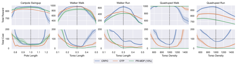
Figure 2: Comparison of algorithms across tasks and environment perturbations. Performance of PR-MDP is evaluated without adversarial interventions. Shading denotes half of one standard error across policies. Vertical dotted lines represent nominal training environment. Top: Total reward. Bottom: Total cost, where horizontal dotted lines represent the safety budget and values below these lines represent safety constraint satisfaction.

We analyze the use of Optimal Transport Perturbations for robust and safe RL on continuous control tasks with safety constraints in the Real-World RL Suite (Dulac-Arnold et al., 2020; 2021). We follow the same experimental design used in Queeney & Benosman (2023). In particular, we consider 5 constrained tasks over 3 domains (Cartpole Swingup, Walker Walk, Walker Run, Quadruped Walk, and Quadruped Run), which all have horizons of $1{,}000$ with $r(s,a)\in[0,1]$ and $c(s,a)\in\left\{0,1\right\}$. In all tasks, we consider a safety budget of $B=100$. We train policies in a nominal training environment for 1 million steps over 5 random seeds, and we evaluate the robustness of the learned policies in terms of both performance and safety across a range of perturbed test environments. See the Appendix for details on the safety constraints and environment perturbations considered for each task.

In our experiments, we consider the safe RL algorithm Constraint-Rectified Policy Optimization (CRPO) (Xu et al., 2021), which immediately switches between maximizing the objective and minimizing the constraint for better constraint satisfaction compared to Lagrangian-based approaches. We use the unconstrained deep RL algorithm Maximum a Posteriori Policy Optimization (MPO) (Abdolmaleki et al., 2018) to calculate policy updates in CRPO. We consider a multivariate Gaussian policy, where the mean and diagonal covariance at a given state are parameterized by a neural network. We also consider separate neural network parameterizations for the reward and cost critics. See the Appendix for additional implementation details, including network architectures and values of all hyperparameters.

We incorporate robustness into this baseline safe RL algorithm in three ways: (i) Optimal Transport Perturbations, (ii) adversarial RL using the action-robust PR-MDP framework from Tessler et al. (2019a) applied to the safety constraint, and (iii) the soft-robust approach of domain randomization (Peng et al., 2018; Derman et al., 2018). For our Optimal Transport Perturbations, we consider the perturbation structure in (15), where $\delta_{r}$ and $\delta_{c}$ are neural networks. We constrain the average per-coordinate magnitude of these perturbation networks to be less than $\epsilon_{\delta}=0.02$ (i.e., 2% perturbations on average).

Figure 2 shows the total rewards and costs obtained by our OTP algorithm for each task across a range of perturbed test environments, compared to CRPO and PR-MDP. The performance of all algorithms averaged across tasks and test environments is summarized in Table 1.

8.1 Comparison to Safe RL

By applying Optimal Transport Perturbations to the objective and constraint in safe RL, we achieve meaningful test-time improvements compared to the standard non-robust version of CRPO. While in most cases we observe a decrease in total rewards in the nominal environment in order to achieve robustness, as expected, on average our framework leads to an increase in total rewards of 1.06x relative to CRPO across the range of test environments. Most importantly, we see a significant improvement in safety, with our algorithm satisfying constraints in 87% of test cases (compared to 51% for CRPO) and incurring 0.34x the costs of CRPO, on average. Note that we achieve this robustness while collecting data from the same training environment considered in CRPO, without requiring adversarial interventions in the environment or domain knowledge on the structure of the perturbed test environments.

8.2 Comparison to Adversarial RL

Next, we compare our approach to the PR-MDP framework (Tessler et al., 2019a), an adversarial RL method that randomly applies adversarial actions a percentage of the time during training. In order to apply this method to the safe RL setting, we train the adversary to maximize costs. We apply the default probability of intervention of 10% considered in Tessler et al. (2019a). As shown in Figure 2, this adversarial approach leads to robust constraint satisfaction across test environments (88% of the time compared to 87% for our OTP framework), especially in the Quadruped environments. Our OTP framework, on the other hand, leads to improved constraint satisfaction in the remaining 3 tasks.

However, the robust safety demonstrated by the PR-MDP approach also results in lower total rewards on average, and is the only robust approach in Table 1 that underperforms CRPO in terms of reward. In order to improve performance with respect to reward, we also considered PR-MDP with a lower probability of intervention of 5%. We include this version of PR-MDP in Table 1, and detailed results across tasks can be found in Figure 4 of the Appendix. While this less adversarial implementation of PR-MDP is comparable to our OTP framework in terms of total rewards, it leads to a decrease in safety constraint satisfaction to 82%. Therefore, our OTP formulation demonstrates the safety benefits of the more adversarial setting and the reward benefits of the less adversarial setting.

In addition, an important drawback of adversarial RL is that it requires the intervention of an adversary in the training environment. Therefore, in order to achieve robust safety at deployment time, the PR-MDP approach incurs additional cost during training due to the presence of an adversary. Even in the Quadruped domains where PR-MDP results in near-zero cost at deployment time, Figure 3 shows that this algorithm leads to the highest total cost during training due to adversarial interventions. In many real-world situations, this additional cost during training is undesirable. Our OTP framework, on the other hand, achieves the lowest total cost during training, while also resulting in robust safety when deployed in perturbed environments. This is due to the fact that our Optimal Transport Perturbations are applied in a completely offline fashion.

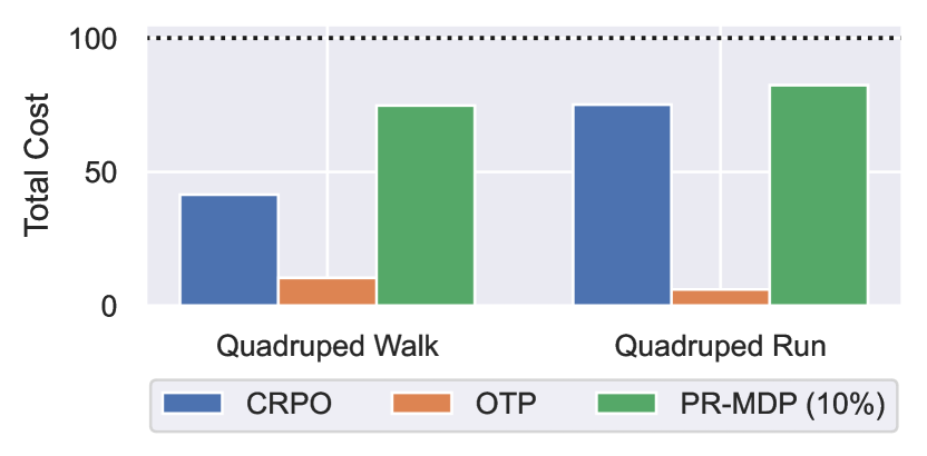
Figure 3: Comparison of average final training cost in the nominal training environment. Training cost of PR-MDP includes impact of adversarial interventions. Horizontal dotted line represents safety budget.

8.3 Comparison to Domain Randomization

Finally, we compare our OTP framework to the soft-robust approach of domain randomization (Peng et al., 2018; Derman et al., 2018), which assumes access to a range of environments during training through the use of a simulator. We consider the same training distributions for domain randomization as in Queeney & Benosman (2023). By training across a range of environments, domain randomization achieves strong performance across test cases in terms of reward (1.14x compared to CRPO, on average), which was the motivation for its development in the setting of sim-to-real transfer. However, note that domain randomization was originally proposed for the unconstrained setting, and we observe that it does not consistently satisfy safety constraints outside of its range of training environments (see Figure 5 in the Appendix). This is likely due to its soft-robust approach that focuses on average performance across the training distribution. Domain randomization satisfies safety constraints in 76% of test cases, which is lower than both OTP and PR-MDP which explicitly consider robust formulations.

It is also important to note that domain randomization not only requires access to a range of training environments, it also requires prior knowledge on the structure of potential disturbances in order to define its training distribution. In order to evaluate the case where we lack domain knowledge, we include an out-of-distribution (OOD) version of domain randomization in Table 1 that is trained on a distribution over a different parameter than the one varied in our perturbed test environments. See Figure 5 in the Appendix for detailed results across tasks. When the training distribution is not appropriately selected, we see that domain randomization provides little benefit compared to standard non-robust safe RL. Our OTP framework, on the other hand, guarantees robust and safe performance under general forms of environment uncertainty while only collecting data from a single training environment.

9 Conclusion

In this work, we have developed a general, efficient framework for robust and safe RL. Through the use of optimal transport theory, we demonstrated that we can guarantee robustness to general forms of environment disturbances by applying adversarial perturbations to observed state transitions. These Optimal Transport Perturbations can be efficiently implemented in an offline fashion using only data collected from a nominal training environment, and can be easily combined with existing techniques for safe RL to provide protection against unknown disturbances.

Because our framework makes limited assumptions on the data collection process during training and does not require directly modifying the environment, it should be compatible with many real-world decision making applications. As a result, we hope that our work represents a promising step towards trustworthy deep RL algorithms that can be reliably deployed to improve real-world decision making.

Appendix A Proofs

Note that

$$\inf_{p_{s,a}\in\mathcal{P}_{s,a}}\mathop{\mathbb{E}}_{s^{\prime}\sim p_{s,a}}\left[V_{r}^{\pi}(s^{\prime})\right]=-\sup_{p_{s,a}\in\mathcal{P}_{s,a}}\mathop{\mathbb{E}}_{s^{\prime}\sim p_{s,a}}\left[-V_{r}^{\pi}(s^{\prime})\right].$$

Therefore, in this section we only prove results for the robust cost Bellman operator $\mathcal{T}^{\pi}_{\mathcal{P},c}$. Results related to the robust reward Bellman operator $\mathcal{T}^{\pi}_{\mathcal{P},r}$ follow immediately by applying the same proofs after an appropriate change in signs.

A.1 Proof of Lemma 5.3

Proof.

Under Assumption 5.1, note that Assumption (A1) and Assumption (A2) of Blanchet & Murthy (2019) are satisfied for the distributionally robust optimization problem in (6). Assumption (A1) is satisfied by our definition of optimal transport cost, and Assumption (A2) is satisfied by our Assumption 5.1. Then, according to Theorem 1 in Blanchet & Murthy (2019), optimal transport strong duality holds for the distributionally robust optimization problem in (6). Therefore, we have that

$$\sup_{p_{s,a}\in\mathcal{P}_{s,a}}\mathop{\mathbb{E}}_{s^{\prime}\sim p_{s,a}}\left[V_{c}^{\pi}(s^{\prime})\right]=\inf_{\lambda\geq 0}\,\,\mathop{\mathbb{E}}_{\hat{s}^{\prime}\sim\hat{p}_{s,a}}\left[\,\,\sup_{s^{\prime}\in\mathcal{S}}\,\,V_{c}^{\pi}(s^{\prime})-\lambda\left(d(\hat{s}^{\prime},s^{\prime})-\epsilon_{s,a}\right)\right].$$

By substituting this result into (6), we arrive at the result in (8). ∎

A.2 Proof of Theorem 5.4

Proof.

First, we write the dual problem to (12) as

$$\inf_{\lambda\geq 0}\,\,\sup_{g\in\mathcal{G}}\,\,\mathop{\mathbb{E}}_{\hat{s}^{\prime}\sim\hat{p}_{s,a}}\left[V_{c}^{\pi}(g(\hat{s}^{\prime}))\right]-\lambda\left(\mathop{\mathbb{E}}_{\hat{s}^{\prime}\sim\hat{p}_{s,a}}\left[d(\hat{s}^{\prime},g(\hat{s}^{\prime}))\right]-\epsilon_{s,a}\right)\\ =\inf_{\lambda\geq 0}\,\,\sup_{g\in\mathcal{G}}\,\,\mathop{\mathbb{E}}_{\hat{s}^{\prime}\sim\hat{p}_{s,a}}\left[V_{c}^{\pi}(g(\hat{s}^{\prime}))-\lambda\left(d(\hat{s}^{\prime},g(\hat{s}^{\prime}))-\epsilon_{s,a}\right)\right].$$

Using the definition of $\mathcal{G}$, we can rewrite this as

$$\inf_{\lambda\geq 0}\,\,\mathop{\mathbb{E}}_{\hat{s}^{\prime}\sim\hat{p}_{s,a}}\left[\,\,\sup_{s^{\prime}\in\mathcal{S}}\,\,V_{c}^{\pi}(s^{\prime})-\lambda\left(d(\hat{s}^{\prime},s^{\prime})-\epsilon_{s,a}\right)\right],$$ (16)

which appears in the right-hand side of (8) from Lemma 5.3. As shown in Lemma 5.3, (16) is also the dual to the distributionally robust optimization problem in (6), and optimal transport strong duality holds.

Next, we show that strong duality holds between (12) and (16). Let $\lambda^{*}$ be the optimal dual variable in (16), and let

$$g^{*}_{s,a}(\hat{s}^{\prime})\in\arg\max_{s^{\prime}\in\mathcal{S}}\,\,V_{c}^{\pi}(s^{\prime})-\lambda^{*}\left(d(\hat{s}^{\prime},s^{\prime})-\epsilon_{s,a}\right).$$

We have that $\lambda^{*}$ and $g^{*}_{s,a}(\hat{s}^{\prime})$ exist according to Theorem 1(b) in Blanchet & Murthy (2019) along with Assumption 5.2, and $g^{*}_{s,a}$ characterizes the optimal transport plan $\nu^{*}$ that moves the probability of $\hat{s}^{\prime}$ under $\hat{p}_{s,a}$ to $g^{*}_{s,a}(\hat{s}^{\prime})$. By the complementary slackness results of Theorem 1(b) in Blanchet & Murthy (2019), we also have that

$$\lambda^{*}\left(\mathop{\mathbb{E}}_{\hat{s}^{\prime}\sim\hat{p}_{s,a}}\left[d(\hat{s}^{\prime},g^{*}_{s,a}(\hat{s}^{\prime}))\right]-\epsilon_{s,a}\right)=0.$$

Therefore,

$$\inf_{\lambda\geq 0}\,\,\mathop{\mathbb{E}}_{\hat{s}^{\prime}\sim\hat{p}_{s,a}}\left[\,\,\sup_{s^{\prime}\in\mathcal{S}}\,\,V_{c}^{\pi}(s^{\prime})-\lambda\left(d(\hat{s}^{\prime},s^{\prime})-\epsilon_{s,a}\right)\right] =\mathop{\mathbb{E}}_{\hat{s}^{\prime}\sim\hat{p}_{s,a}}\left[V_{c}^{\pi}(g^{*}_{s,a}(\hat{s}^{\prime}))-\lambda^{*}\left(d(\hat{s}^{\prime},g^{*}_{s,a}(\hat{s}^{\prime}))-\epsilon_{s,a}\right)\right]$$

$$=\mathop{\mathbb{E}}_{\hat{s}^{\prime}\sim\hat{p}_{s,a}}\left[V_{c}^{\pi}(g^{*}_{s,a}(\hat{s}^{\prime}))\right].$$

Moreover, by the primal feasibility of the optimal transport plan $\nu^{*}$, we have that

$$\mathop{\mathbb{E}}_{\hat{s}^{\prime}\sim\hat{p}_{s,a}}\left[d(\hat{s}^{\prime},g^{*}_{s,a}(\hat{s}^{\prime}))\right]\leq\epsilon_{s,a},$$

so $g^{*}_{s,a}$ is a feasible solution to (12) with the same objective value as the value of (16). Therefore, strong duality holds between (12) and (16), and $g^{*}_{s,a}$ is an optimal solution to (12) (i.e., an optimal solution to (12) exists). Then, for any optimal solution $g^{c}_{s,a}$ to (12), we have that

$$\mathop{\mathbb{E}}_{\hat{s}^{\prime}\sim\hat{p}_{s,a}}\left[V_{c}^{\pi}(g^{c}_{s,a}(\hat{s}^{\prime}))\right]=\mathop{\mathbb{E}}_{\hat{s}^{\prime}\sim\hat{p}_{s,a}}\left[V_{c}^{\pi}(g^{*}_{s,a}(\hat{s}^{\prime}))\right],$$

and the right-hand side of (8) is equivalent to the right-hand side of (10). ∎

Appendix B Implementation Details

B.1 Safety Constraints and Environment Perturbations

Table 2: Safety constraints for all tasks.

		Safety
Task	Safety Constraint	Coefficient
Cartpole Swingup	Slider Position	0.30
Walker Walk	Joint Velocity	0.25
Walker Run	Joint Velocity	0.30
Quadruped Walk	Joint Angle	0.15
Quadruped Run	Joint Angle	0.30

Table 3: Perturbation ranges for test environments across domains.

	Perturbation	Nominal
Domain	Parameter	Value	Test Range
Cartpole	Pole Length	1.00	$\left[0.75,1.25\right]$
Walker	Torso Length	0.30	$\left[0.10,0.50\right]$
Quadruped	Torso Density	$1{,}000$	$\left[500,1{,}500\right]$

Table 4: Perturbation parameters and ranges for domain randomization across domains.

	In-Distribution			Out-of-Distribution
	Perturbation	Nominal	Training	Perturbation	Nominal	Training
Domain	Parameter	Value	Range	Parameter	Value	Range
Cartpole	Pole Length	1.00	$\left[0.875,1.125\right]$	Pole Mass	0.10	$\left[0.05,0.15\right]$
Walker	Torso Length	0.30	$\left[0.20,0.40\right]$	Contact Friction	0.70	$\left[0.40,1.00\right]$
Quadruped	Torso Density	$1{,}000$	$\left[750,1{,}250\right]$	Contact Friction	1.50	$\left[1.00,2.00\right]$

We consider the same experimental design used in Queeney & Benosman (2023) to define our training and test environments. For each task, we consider a single safety constraint defined in the Real-World RL Suite, which we summarize in Table 2. A policy incurs cost in the Cartpole domain when the slider moves outside of a specified range, in the Walker domain when the velocity of any joint exceeds a threshold, and in the Quadruped domain when joint angles are outside of an acceptable range. The specific ranges that result in cost violations are determined by the safety coefficients in Table 2, which can take values in $\left[0,1\right]$ where lower values make cost violations more likely. See Dulac-Arnold et al. (2021) for detailed definitions of the safety constraints we consider.

We evaluate the performance of learned policies across a range of test environments different from the training environment. We define these test environments by varying a simulator parameter in each domain across a range of values, which are listed in Table 3. We vary the length of the pole in the Cartpole domain, the length of the torso in the Walker domain, and the density of the torso in the Quadruped domain. Note that the parameter value associated with the nominal training environment is in the center of the range of parameter values considered at test time.

Finally, note that the domain randomization baselines consider a range of environments during training. As summarized in Table 4, in-distribution domain randomization applies a uniform distribution over the middle 50% of the parameter values considered at test time. In the out-of-distribution variant of domain randomization, we instead consider a uniform distribution over a range of values for a different simulator parameter than the one varied at test time. See Table 4 for details.

B.2 Network Architectures

Table 5: Network architectures and algorithm hyperparameters used in experiments.

General
Batch size per update		256
Updates per environment step		1
Discount rate ($\gamma$)		0.99
Target network exponential moving average ($\tau$)		5e-3
Policy
Layer sizes		256, 256, 256
Layer activations		ELU
Layer norm + tanh on first layer		Yes
Initial standard deviation		0.3
Learning rate		1e-4
Non-parametric KL ($\epsilon_{\textnormal{KL}}$)		0.10
Action penalty KL		1e-3
Action samples per update		20
Parametric mean KL ($\beta_{\mu}$)		0.01
Parametric covariance KL ($\beta_{\Sigma}$)		1e-5
Parametric KL dual learning rate		0.01
Critics
Layer sizes		256, 256, 256
Layer activations		ELU
Layer norm + tanh on first layer		Yes
Learning rate		1e-4

In our experiments, we consider neural network representations of the policy and critics. We consider networks with 3 hidden layers of 256 units and ELU activations, and we apply layer normalization followed by a tanh activation after the first layer as in Abdolmaleki et al. (2020). We represent the policy as a multivariate Gaussian distribution with diagonal covariance, where at a given state the policy network outputs the mean $\mu(s)$ and diagonal covariance $\Sigma(s)$ of the action distribution. The diagonal of $\Sigma(s)$ is calculated by applying the softplus operator to the outputs of the neural network corresponding to the covariance. In addition to the policy network, we consider separate networks for the reward and cost critics. We maintain target versions of the policy and critic networks using an exponential moving average of the weights with $\tau=5{e-}3$. Finally, we also consider neural networks for our perturbation networks $\delta_{r}$ and $\delta_{c}$. In this work, we consider small networks with 2 hidden layers of 64 units and ELU activations. We clip the outputs in the range $\left[-2\epsilon_{\delta},2\epsilon_{\delta}\right]$ for additional stability.

B.3 Algorithm Hyperparameters

All of the algorithms in our experiments build upon the baseline safe RL algorithm CRPO (Xu et al., 2021). At every update, CRPO calculates the current value of the safety constraint based on a batch of sampled data. If the safety constraint is satisfied for the current batch, it applies a policy update to maximize rewards. Otherwise, it applies a policy update to minimize costs. In both cases, we use the unconstrained RL algorithm MPO (Abdolmaleki et al., 2018) to calculate policy updates. MPO calculates a non-parametric target policy with KL divergence $\epsilon_{\textnormal{KL}}$ from the current policy, and updates the current policy towards this target while constraining separate KL divergence contributions from the mean and covariance by $\beta_{\mu}$ and $\beta_{\Sigma}$, respectively. We apply per-dimension KL divergence constraints and action penalization using the multi-objective MPO framework (Abdolmaleki et al., 2020) as in Hoffman et al. (2020), and we consider closed-form updates of the temperature parameter used in the non-parametric target policy as in Liu et al. (2022) to account for the immediate switching between objectives in CRPO. See Table 5 for all important hyperparameter values associated with the implementation of policy updates using MPO, and see Abdolmaleki et al. (2018) for additional details.

For our OTP framework, we update the perturbation networks alongside the policy and critics. In particular, we consider a constraint on the average per-coordinate magnitude of the outputs of $\delta_{r}$ and $\delta_{c}$ determined by the parameter $\epsilon_{\delta}$, and we apply gradient-based updates on the Lagrangian relaxations of (13) and (14) using this constraint. We also update the corresponding dual variables throughout training.

Finally, we also implement PR-MDP and domain randomization using CRPO with MPO policy updates. The adversary in PR-MDP is updated using MPO with the goal of maximizing costs. Using the default settings from Tessler et al. (2019a), we apply one adversary update for every 10 policy updates. Domain randomization considers the same updates as the CRPO baseline, but collects data from the range of training environments summarized in Table 4.

Table 6: Network architectures and hyperparameters for Optimal Transport Perturbations.

Optimal Transport Perturbations
Layer sizes		64, 64
Layer activations		ELU
Layer norm + tanh on first layer		No
Output clipping		$\left[-2\epsilon_{\delta},2\epsilon_{\delta}\right]$
Learning rate		1e-4
Dual learning rate		0.01
Per-coordinate perturbation magnitude ($\epsilon_{\delta}$)		0.02

Appendix C Detailed Experimental Results

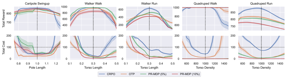
Figure 4: Comparison with adversarial RL. Performance of PR-MDP is evaluated without adversarial interventions. Shading denotes half of one standard error across policies. Vertical dotted lines represent nominal training environment. Top: Total reward. Bottom: Total cost, where horizontal dotted lines represent the safety budget and values below these lines represent safety constraint satisfaction.

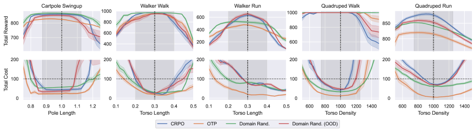
Figure 5: Comparison with domain randomization. Shading denotes half of one standard error across policies. Grey shaded area denotes range of training distribution for in-distribution version of domain randomization. Vertical dotted lines represent nominal training environment. Top: Total reward. Bottom: Total cost, where horizontal dotted lines represent the safety budget and values below these lines represent safety constraint satisfaction.

In this section, we include detailed results across tasks and test environments for all algorithms listed in Table 1. Figure 4 shows the performance of both variations of the adversarial PR-MDP approach using different probabilities of adversary intervention. In general, the less adversarial PR-MDP implementation with 5% intervention probability achieves similar total reward to OTP across all tasks. While this implementation continues to generate strong, safe performance in the Quadruped domains, it does not lead to robust constraint satisfaction in other tasks such as Cartpole Swingup and Walker Run. Our OTP framework, on the other hand, results in consistent constraint satisfaction in these tasks.

Figure 5 shows the performance of domain randomization across tasks and environment perturbations. The grey shaded area represents the range of training distributions for the in-distribution implementation of domain randomization. We see that domain randomization leads to strong, robust performance in terms of rewards across all test cases, as well as improved constraint satisfaction in perturbed environments compared to CRPO. However, in tasks such as Walker Run and Quadruped Run, domain randomization does not robustly satisfy safety constraints for test environments that were not seen during training. This issue is amplified in the case of out-of-distribution domain randomization, which does not demonstrate consistent robustness benefits compared to standard safe RL. In fact, it even leads to an increase in constraint-violating test cases in Cartpole Swingup compared to CRPO. This demonstrates that training on multiple environments does not necessarily lead to robust performance. Instead, domain knowledge is critical in order for domain randomization to work well in practice.

References

- Abdolmaleki et al. (2018) Abdolmaleki, A., Springenberg, J. T., Tassa, Y., Munos, R., Heess, N., and Riedmiller, M. Maximum a posteriori policy optimisation. In Sixth International Conference on Learning Representations, 2018.
- Abdolmaleki et al. (2020) Abdolmaleki, A., Huang, S., Hasenclever, L., Neunert, M., Song, F., Zambelli, M., Martins, M., Heess, N., Hadsell, R., and Riedmiller, M. A distributional view on multi-objective policy optimization. In Proceedings of the 37th International Conference on Machine Learning, volume 119, pp. 11–22. PMLR, 2020.
- Abdullah et al. (2019) Abdullah, M. A., Ren, H., Ammar, H. B., Milenkovic, V., Luo, R., Zhang, M., and Wang, J. Wasserstein robust reinforcement learning. arXiv preprint, 2019. arXiv:1907.13196.
- Achiam et al. (2017) Achiam, J., Held, D., Tamar, A., and Abbeel, P. Constrained policy optimization. In Proceedings of the 34th International Conference on Machine Learning, volume 70, pp. 22–31. PMLR, 2017.
- Altman (1999) Altman, E. Constrained Markov Decision Processes. CRC Press, 1999.
- Bharadhwaj et al. (2021) Bharadhwaj, H., Kumar, A., Rhinehart, N., Levine, S., Shkurti, F., and Garg, A. Conservative safety critics for exploration. In Ninth International Conference on Learning Representations, 2021.
- Blanchet & Murthy (2019) Blanchet, J. and Murthy, K. Quantifying distributional model risk via optimal transport. Mathematics of Operations Research, 44(2):565–600, 2019. doi: 10.1287/moor.2018.0936.
- Cheng et al. (2019) Cheng, R., Orosz, G., Murray, R. M., and Burdick, J. W. End-to-end safe reinforcement learning through barrier functions for safety-critical continuous control tasks. In Proceedings of the AAAI Conference on Artificial Intelligence, volume 33, pp. 3387–3395. AAAI Press, 2019.
- Dalal et al. (2018) Dalal, G., Dvijotham, K., Vecerik, M., Hester, T., Paduraru, C., and Tassa, Y. Safe exploration in continuous action spaces. arXiv preprint, 2018. arXiv:1801.08757.
- Derman et al. (2018) Derman, E., Mankowitz, D. J., Mann, T. A., and Mannor, S. Soft-robust actor-critic policy-gradient. arXiv preprint, 2018. arXiv:1803.04848.
- Dulac-Arnold et al. (2020) Dulac-Arnold, G., Levine, N., Mankowitz, D. J., Li, J., Paduraru, C., Gowal, S., and Hester, T. An empirical investigation of the challenges of real-world reinforcement learning. arXiv preprint, 2020. arXiv:2003.11881.
- Dulac-Arnold et al. (2021) Dulac-Arnold, G., Levine, N., Mankowitz, D. J., Li, J., Paduraru, C., Gowal, S., and Hester, T. Challenges of real-world reinforcement learning: definitions, benchmarks and analysis. Machine Learning, 110:2419–2468, 2021. doi: 10.1007/s10994-021-05961-4.
- Emam et al. (2021) Emam, Y., Glotfelter, P., Kira, Z., and Egerstedt, M. Safe model-based reinforcement learning using robust control barrier functions. arXiv preprint, 2021. arXiv:2110.05415.
- Hoffman et al. (2020) Hoffman, M. W., Shahriari, B., Aslanides, J., Barth-Maron, G., Momchev, N., Sinopalnikov, D., Stańczyk, P., Ramos, S., Raichuk, A., Vincent, D., Hussenot, L., Dadashi, R., Dulac-Arnold, G., Orsini, M., Jacq, A., Ferret, J., Vieillard, N., Ghasemipour, S. K. S., Girgin, S., Pietquin, O., Behbahani, F., Norman, T., Abdolmaleki, A., Cassirer, A., Yang, F., Baumli, K., Henderson, S., Friesen, A., Haroun, R., Novikov, A., Colmenarejo, S. G., Cabi, S., Gulcehre, C., Paine, T. L., Srinivasan, S., Cowie, A., Wang, Z., Piot, B., and de Freitas, N. Acme: A research framework for distributed reinforcement learning. arXiv preprint, 2020. arXiv:2006.00979.
- Hou et al. (2020) Hou, L., Pang, L., Hong, X., Lan, Y., Ma, Z., and Yin, D. Robust reinforcement learning with Wasserstein constraint. arXiv preprint, 2020. arXiv:2006.00945.
- Iyengar (2005) Iyengar, G. N. Robust dynamic programming. Mathematics of Operations Research, 30(2):257–280, 2005. doi: 10.1287/moor.1040.0129.
- Kuang et al. (2022) Kuang, Y., Lu, M., Wang, J., Zhou, Q., Li, B., and Li, H. Learning robust policy against disturbance in transition dynamics via state-conservative policy optimization. In Proceedings of the AAAI Conference on Artificial Intelligence, volume 36, pp. 7247–7254, 2022.
- Liu et al. (2022) Liu, Z., Cen, Z., Isenbaev, V., Liu, W., Wu, S., Li, B., and Zhao, D. Constrained variational policy optimization for safe reinforcement learning. In Proceedings of the 39th International Conference on Machine Learning, pp. 13644–13668. PMLR, 2022.
- Ma et al. (2021) Ma, H., Chen, J., Eben, S., Lin, Z., Guan, Y., Ren, Y., and Zheng, S. Model-based constrained reinforcement learning using generalized control barrier function. In 2021 IEEE/RSJ International Conference on Intelligent Robots and Systems (IROS), pp. 4552–4559, 2021. doi: 10.1109/IROS51168.2021.9636468.
- Mandlekar et al. (2017) Mandlekar, A., Zhu, Y., Garg, A., Fei-Fei, L., and Savarese, S. Adversarially robust policy learning: Active construction of physically-plausible perturbations. In 2017 IEEE/RSJ International Conference on Intelligent Robots and Systems (IROS), pp. 3932–3939, 2017. doi: 10.1109/IROS.2017.8206245.
- Mankowitz et al. (2020) Mankowitz, D. J., Levine, N., Jeong, R., Abdolmaleki, A., Springenberg, J. T., Shi, Y., Kay, J., Hester, T., Mann, T., and Riedmiller, M. Robust reinforcement learning for continuous control with model misspecification. In Eighth International Conference on Learning Representations, 2020.
- Mankowitz et al. (2021) Mankowitz, D. J., Calian, D. A., Jeong, R., Paduraru, C., Heess, N., Dathathri, S., Riedmiller, M., and Mann, T. Robust constrained reinforcement learning for continuous control with model misspecification. arXiv preprint, 2021. arXiv:2010.10644.
- Nilim & Ghaoui (2005) Nilim, A. and Ghaoui, L. E. Robust control of Markov decision processes with uncertain transition matrices. Operations Research, 53(5):780–798, 2005. doi: 10.1287/opre.1050.0216.
- Paternain et al. (2019) Paternain, S., Chamon, L., Calvo-Fullana, M., and Ribeiro, A. Constrained reinforcement learning has zero duality gap. In Advances in Neural Information Processing Systems, volume 32. Curran Associates, Inc., 2019.
- Peng et al. (2018) Peng, X. B., Andrychowicz, M., Zaremba, W., and Abbeel, P. Sim-to-real transfer of robotic control with dynamics randomization. In 2018 IEEE International Conference on Robotics and Automation (ICRA), pp. 3803–3810, 2018. doi: 10.1109/ICRA.2018.8460528.
- Pinto et al. (2017) Pinto, L., Davidson, J., Sukthankar, R., and Gupta, A. Robust adversarial reinforcement learning. In Proceedings of the 34th International Conference on Machine Learning, volume 70, pp. 2817–2826. PMLR, 2017.
- Pydi & Jog (2020) Pydi, M. S. and Jog, V. Adversarial risk via optimal transport and optimal couplings. In Proceedings of the 37th International Conference on Machine Learning, volume 119, pp. 7814–7823. PMLR, 2020.
- Queeney & Benosman (2023) Queeney, J. and Benosman, M. Risk-averse model uncertainty for distributionally robust safe reinforcement learning. arXiv preprint, 2023. arXiv:2301.12593.
- Rajeswaran et al. (2017) Rajeswaran, A., Ghotra, S., Ravindran, B., and Levine, S. EPOpt: Learning robust neural network policies using model ensembles. In 5th International Conference on Learning Representations, 2017.
- Ray et al. (2019) Ray, A., Achiam, J., and Amodei, D. Benchmarking safe exploration in in deep reinforcement learning, 2019.
- Russel et al. (2021) Russel, R. H., Benosman, M., Van Baar, J., and Corcodel, R. Lyapunov robust constrained-MDPs: Soft-constrained robustly stable policy optimization under model uncertainty. arXiv preprint, 2021. arXiv:2108.02701.
- Srinivasan et al. (2020) Srinivasan, K., Eysenbach, B., Ha, S., Tan, J., and Finn, C. Learning to be safe: Deep RL with a safety critic. arXiv preprint, 2020. arXiv:2010.14603.
- Stooke et al. (2020) Stooke, A., Achiam, J., and Abbeel, P. Responsive safety in reinforcement learning by PID Lagrangian methods. In Proceedings of the 37th International Conference on Machine Learning, volume 119, pp. 9133–9143. PMLR, 2020.
- Tessler et al. (2019a) Tessler, C., Efroni, Y., and Mannor, S. Action robust reinforcement learning and applications in continuous control. In Proceedings of the 36th International Conference on Machine Learning, volume 97, pp. 6215–6224. PMLR, 2019a.
- Tessler et al. (2019b) Tessler, C., Mankowitz, D. J., and Mannor, S. Reward constrained policy optimization. In Seventh International Conference on Learning Representations, 2019b.
- Thananjeyan et al. (2021) Thananjeyan, B., Balakrishna, A., Nair, S., Luo, M., Srinivasan, K., Hwang, M., Gonzalez, J. E., Ibarz, J., Finn, C., and Goldberg, K. Recovery RL: Safe reinforcement learning with learned recovery zones. IEEE Robotics and Automation Letters, 6(3):4915–4922, 2021. doi: 10.1109/LRA.2021.3070252.
- Tobin et al. (2017) Tobin, J., Fong, R., Ray, A., Schneider, J., Zaremba, W., and Abbeel, P. Domain randomization for transferring deep neural networks from simulation to the real world. In 2017 IEEE/RSJ International Conference on Intelligent Robots and Systems (IROS), pp. 23–30, 2017. doi: 10.1109/IROS.2017.8202133.
- Villani (2008) Villani, C. Optimal transport, old and new. Springer, 2008. doi: 10.1007/978-3-540-71050-9.
- Vinitsky et al. (2020) Vinitsky, E., Du, Y., Parvate, K., Jang, K., Abbeel, P., and Bayen, A. Robust reinforcement learning using adversarial populations. arXiv preprint, 2020. arXiv:2008.01825.
- Wagener et al. (2021) Wagener, N. C., Boots, B., and Cheng, C.-A. Safe reinforcement learning using advantage-based intervention. In Proceedings of the 38th International Conference on Machine Learning, volume 139, pp. 10630–10640. PMLR, 2021.
- Xu et al. (2022) Xu, M., Liu, Z., Huang, P., Ding, W., Cen, Z., Li, B., and Zhao, D. Trustworthy reinforcement learning against intrinsic vulnerabilities: Robustness, safety, and generalizability. arXiv preprint, 2022. arXiv:2209.08025.
- Xu et al. (2021) Xu, T., Liang, Y., and Lan, G. CRPO: A new approach for safe reinforcement learning with convergence guarantee. In Proceedings of the 38th International Conference on Machine Learning, pp. 11480–11491. PMLR, 2021.
- Zhang et al. (2020) Zhang, H., Chen, H., Xiao, C., Li, B., Liu, M., Boning, D., and Hsieh, C.-J. Robust deep reinforcement learning against adversarial perturbations on state observations. In Advances in Neural Information Processing Systems, volume 33, pp. 21024–21037. Curran Associates, Inc., 2020.