Misspecification-robust Sequential Neural Likelihood

Abstract

Simulation-based inference (SBI) techniques are now an essential tool for the parameter estimation of mechanistic and simulatable models with intractable likelihoods. Statistical approaches to SBI such as approximate Bayesian computation and Bayesian synthetic likelihood have been well studied in the well specified and misspecified settings. However, most implementations are inefficient in that many model simulations are wasted. Neural approaches such as sequential neural likelihood (SNL) have been developed that exploit all model simulations to build a surrogate of the likelihood function. However, SNL approaches have been shown to perform poorly under model misspecification. In this paper, we develop a new method for SNL that is robust to model misspecification and can identify areas where the model is deficient. We demonstrate the usefulness of the new approach on several illustrative examples.

Keywords: generative models, implicit models, likelihood-free inference, normalising flows, simulation-based inference

1 Introduction

Statistical inference for complex models can be challenging when the likelihood function is infeasible to evaluate many times. However, if the model is computationally inexpensive to simulate given parameter values, it is possible to perform approximate parameter estimation by so-called simulation-based inference (SBI) techniques (e.g. Cranmer et al., (2020)). The difficulty of obtaining reliable inferences in the SBI setting is exacerbated when the model is misspecified (e.g. Frazier et al., (2020)).

Statistical approaches for SBI, such as approximate Bayesian computation (ABC, Sisson et al., (2018)) and Bayesian synthetic likelihood (BSL, Price et al., (2018)) have been well studied, both empirically (e.g. Drovandi and Frazier, (2022)) and theoretically (e.g. Li and Fearnhead, (2018), Frazier et al., (2018), Frazier et al., (2022)). These approaches often base inference on a summarisation of the data to manage computational costs. ABC aims to minimise the distance between observed and simulated summaries, whereas BSL constructs a Gaussian approximation of the model summary to form an approximate likelihood. In the case of model misspecification, there may be additional motivation to replace the entire dataset with summaries, as the resulting model can then be trained to capture the broad features of the data that may be of most interest; see, e.g., Lewis et al., (2021) for further discussion. In this paper, the type of misspecification we are interested in is when the model is not able to recover the observed summary statistic as the sample size diverges. This form of misspecification is referred to as incompatibility in Marin et al., (2014).

The behaviour of ABC and BSL under incompatibility is now well understood. Frazier et al., (2020) show that under various assumptions, ABC is capable of concentrating onto the pseudo-true parameter value, which in the SBI context is the value that minimises some distance between the large sample limit of the observed and simulated summaries. However, the concentration is not Gaussian and credible intervals do not have the correct frequentist coverage. BSL on the other hand can exhibit unexpected behaviour under misspecification (Frazier et al.,, 2021). For example, it is possible to obtain Gaussian concentration onto the pseudo-true parameter, but it is also possible to obtain a multi-modal posterior that does not concentrate onto a singleton. Unfortunately, the behaviour for a given problem is not known a priori.

Given the undesirable properties of BSL under misspecification, Frazier and Drovandi, (2021) propose methods to simultaneously identify which statistics are incompatible and make inferences robust. The approach of Frazier and Drovandi, (2021) is a model expansion that introduces auxiliary variables, one per summary statistic, whose purpose is to either shift the means or inflate the variances in the Gaussian approximation so that the extended model is compatible, i.e. to soak up the misspecification.

Although ABC is, in a certain sense, robust to misspecification, and BSL has been extended to handle incompatibility, they both remain inefficient in terms of the number of model simulations required. Most algorithms for ABC and BSL are wasteful in the sense they use a relatively large number of model simulations that are associated with rejected parameter proposals (for some exceptions to this, see Jasra et al., (2019); Levi and Craiu, (2022); Warne et al., (2018, 2022)). This has motivated the development of methods in machine learning that utilise all model simulations to learn either the likelihood (e.g. Papamakarios et al., (2019)), posterior (e.g. Greenberg et al., (2019)) or likelihood ratio (e.g. Thomas et al., (2022)). Since these objects are learned as functions of the parameter, subsequent posterior inference does not require further model simulation.

However, the machine learning approaches, such as sequential neural likelihood (SNL) and sequential neural posterior (SNP) have been shown to exhibit poor performance under model misspecification (e.g. Bon et al., (2022); Cannon et al., (2022); Schmitt et al., (2021); Ward et al., (2022)). Thus there is a critical need to develop these neural approaches so they are robust to model misspecification. Ward et al., (2022) develop a method, which shares similarities to the mean adjustment approach developed for BSL, to make neural posterior estimation robust to model misspecification. Cannon et al., (2022) develop several neural SBI robust methods by incorporating machine learning methods that are known to better handle out-of-distribution (OOD) data. Cranmer et al., (2020) advise to incorporate additional noise directly into the simulator if model misspecification is suspected.

In this paper we develop a robust version of SNL, again inspired by the mean adjustment approach for BSL. Unlike Ward et al., (2022) who consider neural posterior estimation, we consider neural likelihood estimation, which is useful for problems where the likelihood is easier to emulate compared to the posterior. Further, ours is the first sequential neural approach that simultaneously detects and corrects for model misspecification.

2 Background

Let $y=(y_{1},\dots,y_{n})^{\top}$ denote the observed data and define $P^{(n)}_{0}$ as the true distribution of $y$. The observed data is assumed to be generated from a class of parametric models $\{P^{(n)}_{\theta}:\theta\in\Theta\subset\mathbb{R}^{d_{\theta}}\}$ for which the likelihood function is intractable, but from which we can easily simulate pseudo-data $x$ for any $\theta\in\Theta$ where $\theta$ is $d_{\theta}$ dimensional. Let $\Pi$ denote the prior measure for $\theta$ and $\pi({\theta})$ its density. The posterior density of interest is given by

$$\pi(\theta\mid y)\propto g(y\mid\theta)\pi(\theta),$$

where $g(y\mid\theta)$ is the likelihood function.

2.1 Statistical Approaches for SBI

Since we assume that the likelihood is computationally intractable, we conduct inference using approximate Bayesian methods. Statistical approaches to SBI aim to search for values of $\theta$ that produce pseudo-data $x$ which is “close enough” to $y$, and then retain these values to build an approximation to the posterior. To ensure the problem is computationally practical, the comparison is generally carried out using summaries of the data. Moreover, under model misspecification, there may be further motivation to conduct inference based on summaries, to attempt to capture the key features of the data. Let $S:\mathbb{R}^{n}\rightarrow\mathbb{R}^{d}$, $d\geq d_{\theta}$, denote the vector summary statistic mapping used in the analysis.

Two prominent statistical approaches for SBI are ABC and BSL. ABC approximates the likelihood via the following:

$$g_{\epsilon}({S(y)\mid\theta})=\int_{\mathbb{R}^{d}}K_{\epsilon}(\rho\{S(y),S(x)\})g_{n}({S(x)\mid\theta})dx,$$

where $\rho\{S(y),S(x)\}$ measures the discrepancy between observed and simulated summaries and $K_{\epsilon}(\cdot)$ is a kernel that allocates higher weight to smaller $\rho$. The bandwidth of the kernel, $\epsilon$, is often referred to as the tolerance in the ABC literature. The above integral is intractable, but can be estimated unbiasedly by drawing $m$ mock datasets $x_{1},\ldots,x_{m}\sim P^{(n)}_{\theta}$ and computing

$$\hat{g}_{\epsilon}({S(y)\mid\theta})=\frac{1}{m}\sum_{i=1}^{m}K_{\epsilon}(\rho\{S(y),S(x_{i})\}).$$

It is common to set $m=1$ and choose the indicator kernel function, $K_{\epsilon}(\rho\{S(y),S(x)\})=\mathbf{I}(\rho\{S(y),S(x)\}\leq\epsilon)$. Using arguments from the exact-approximate literature (Andrieu and Roberts,, 2009), unbiasedly estimating the ABC likelihood leads to a Bayesian algorithm that samples from the approximate posterior proportional to $g_{\epsilon}({S(y)\mid\theta})\pi(\theta)$.

As is evident from the above integral estimator, ABC non-parametrically estimates the summary statistic likelihood. In contrast, BSL uses a parametric estimator. The most common BSL approach approximates $g_{n}(\cdot\mid\theta)$ using a Gaussian:

$$g_{A}({S(y)\mid\theta})=\mathcal{N}\left(S(y);\mu(\theta),\Sigma(\theta)\right),$$

where $\mu(\theta)=\mathsf{E}[S(x)|\theta]$ and $\Sigma(\theta)=\mbox{Var}(S(x)|\theta)$ denote the mean and variance of the model summary statistic at $\theta$. In almost all practical cases $\mu(\theta)$ and $\Sigma(\theta)$ are unknown, but we can replace these quantities with those estimated from $m$ independent model simulations, using for example the sample mean and variance:

$$\mu_{m}(\theta) =\frac{1}{m}\sum_{i=1}^{m}S(x^{i}),$$

$$\Sigma_{m}(\theta) =\frac{1}{m}\sum_{i=1}^{m}\left(S(x^{i})-\mu_{m}(\theta)\right)\left(S(x^{i})-\mu_{m}(\theta)\right)^{\top},$$

and where each simulated data set $x^{i}$, $i=1,\dots,m$, is generated iid from $P^{(n)}_{\theta}$. The synthetic likelihood is then approximated as

$$\hat{g}_{A}({S(y)\mid\theta})=\mathcal{N}\left(S(y);\mu_{m}(\theta),\Sigma_{m}(\theta)\right).$$

Unlike ABC, $\hat{g}_{A}({S(y)\mid\theta})$ is not an unbiased estimator of $g_{A}(S(y)\mid\theta)$. Frazier et al., (2022) demonstrate that if the summary statistics are sub-Gaussian, then the choice of $m$ is immaterial so long as $m$ diverges as $n$ diverges. The insensitivity to $m$ is supported empirically in Price et al., (2018), provided that $m$ is chosen large enough so that the plug-in synthetic likelihood estimator has a small enough variance to ensure that MCMC mixing is not adversely affected.

2.2 SBI and Model Misspecification

The usual notion of model misspecification is not meaningful in the SBI context, i.e., no value of $\theta\in\Theta$ such that $P^{(n)}_{\theta}=P_{0}^{(n)}$, since even if the model is incorrect, it is still possible that $P^{(n)}_{\theta}$ can generate summary statistics that match the observed statistic (Frazier et al.,, 2020). Define $b(\theta)=\mathsf{E}[S(x)\mid\theta]$ and $b_{0}=\mathsf{E}[S(y)]$ as the expected value of the summary statistic with respect to the probability measures $P^{(n)}_{\theta}$ and $P^{(n)}_{0}$, respectively. That is, the expectations are with respect to the model conditioned on $\theta$ and the true data generating process, respectively. The meaningful notion of misspecification in the SBI context is when there is no $\theta\in\Theta$ such that $b(\theta)=b_{0}$, i.e. there is no parameter value such that the expected simulated and observed summaries match.

In the context of ABC, we say that the model is misspecified if

$$\epsilon^{*}=\inf_{\theta\in\Theta}\rho(b(\theta),b_{0})>0,$$

for some metric $\rho$, and the corresponding pseudo-true parameter is defined as $\theta^{*}=\arg\inf_{\theta\in\Theta}\rho(b(\theta),b_{0})$. Frazier et al., (2020) show, under various conditions, the ABC posterior concentrates onto $\theta^{*}$ for large sample sizes, and thus ABC does possess an inherent robustness to model misspecification. However, Frazier et al., (2020) also show that the asymptotic shape of the ABC posterior is non-Gaussian and credible intervals do not possess valid frequentist coverage; i.e., confidence sets do not have the correct level under $P^{(n)}_{0}$.

In the context of BSL, Frazier et al., (2021) show that when the model is incompatible, i.e. $b(\theta)\neq b_{0}$ $\forall\theta\in\Theta$, the Kullback-Leibler divergence between the true data generating distribution and the Gaussian distribution associated with the synthetic likelihood diverges as $n$ diverges. In BSL, we say that the model is incompatible if

$$\lim_{n\rightarrow\infty}\inf_{\theta\in\Theta}\left\{b(\theta)-b_{0}\right\}^{\top}\left\{n\Sigma(\theta)\right\}^{-1}\left\{b(\theta)-b_{0}\right\}>0.$$

Define $M_{n}(\theta)=n^{-1}\partial\log g_{A}\left(S\mid\theta\right)/\partial\theta$. The behaviour of BSL under misspecification is dependent on the number of roots of $M_{n}(\theta)=0$. If there is a single solution, and under various assumptions, the BSL posterior will concentrate onto the pseudo-true parameter $\theta^{*}$ and its asymptotic shape is Gaussian, and the BSL posterior mean satisfies a Bernstein von-Mises result. However, if there are multiple solutions to $M_{n}(\theta)=0$, then the BSL posterior will asymptotically exhibit multiple modes that do not concentrate on $\theta^{*}$. The number of solutions to $M_{n}(\theta)=0$ for a given problem is not known a priori and is very difficult to explore.

In addition to the theoretical issues suffered by BSL under misspecification, there is also computational issues. Frazier and Drovandi, (2021) identify that, under incompatibility, since the observed summary lies in the tail of the estimated synthetic likelihood for any value of $\theta$, the Monte Carlo estimate of the likelihood suffers from high variance. Consequently, a very large value of $m$ is required to allow the MCMC chain to mix and not become stuck, which is computationally burdensome.

A solution to the BSL incompatibility problem is provided in Frazier and Drovandi, (2021). The solution involves expanding the model to include an auxiliary parameter, $\Gamma\in\mathbb{R}^{d}$ such that $\Gamma=(\gamma_{1},\ldots,\gamma_{d})^{\top}$, which has the same dimension as the summary statistic. The approach of Frazier and Drovandi, (2021) then either adjusts the mean or inflates the variance of the synthetic likelihood so that the observed summary does not lie so far in the tails of the expanded model. The expanded model is overparameterised since $\dim((\theta,\Gamma)^{\top})=d+d_{\theta}$, which is greater than the dimension of the summary statistic, $d$. To regularise the model, Frazier and Drovandi, (2021) impose a prior distribution on $\Gamma$ that favours compatibility. However, the prior for each component of $\Gamma$ has a heavy tail so that it can “soak up” the misspecification for a certain subset of the summary statistics. By doing so, the method is able to identify the statistics that the model is not compatible with, and at the same time, mitigate the influence of the incompatible statistics on the inference. Frazier and Drovandi, (2021) show that under compatibility, the posterior for $\Gamma$ is the same as its prior, so that incompatibility can be detected by departures from the prior.

Here we provide more detail on the mean adjustment method of Frazier and Drovandi, (2021) since we adopt a similar approach within our robust SNL method. The mean adjusted (estimated) synthetic likelihood is denoted

$$\mathcal{N}\left(S;\mu_{m}(\theta)+\sigma_{m}(\theta)\circ\Gamma,\Sigma_{m}(\theta)\right),$$

where $\sigma_{m}(\theta)$ is the vector of estimated standard deviations of the model summary statistics, and $\circ$ denotes the Hadamard (element-by-element) product. The role of $\sigma_{m}(\theta)$ is to ensure that we can treat each component of $\Gamma$ as the number of standard deviations (either positive or negative) that we are shifting the corresponding model summary statistic. Frazier and Drovandi, (2021) suggest using a prior for which $\theta$ and $\Gamma$ are independent, with the prior density for $\Gamma$ being

$$p(\Gamma)=\prod_{j=1}^{d}\frac{1}{2\lambda}\exp\left(-\frac{|\gamma_{j}|}{\lambda}\right).$$

The Laplace prior above with scale $\lambda$ for each $\gamma_{j}$ is chosen because it is peaked at zero, but with a moderately heavy tail. Frazier and Drovandi, (2021) develop a component-wise MCMC algorithm that iteratively updates via the conditionals $\theta|S,\Gamma$ and $\Gamma|S,\theta$. The update for $\Gamma$ holds the $m$ model simulations fixed and uses a slice sampler so that the acceptance rate is one and does not requiring tuning a proposal distribution. Frazier and Drovandi, (2021) find empirically that sampling over the joint space $(\theta,\Gamma)^{\top}$ does not slow down mixing on the $\theta$-marginal space. On the contrary, in the case of misspecification, the mixing is substantially improved as the observed value of the summaries no longer falls in the tail of the Gaussian distribution.

Although ABC has a natural robustness to misspecification and BSL has been extended to accommodate incompatibility, both methods reject a large number of model simulations, and can thus be highly computationally intensive when simulating the model is not cheap. As described in the introduction, neural methods in the machine learning community have been developed that exploit all the model simulations to build a surrogate model of the posterior, likelihood or likelihood ratio. Below we describe one of these methods, sequential neural likelihood (SNL), and show how it can be extended to accommodate model misspecification.

3 Robust Sequential Neural Likelihood

In this section, we propose an approach that extends SNL using a similar method to the mean adjustment approach in Frazier and Drovandi, (2021) so that it is robust to model misspecification.

3.1 Sequential Neural Likelihood

SNL belongs to the class of SBI methods that use a neural conditional density estimator (NCDE). A NCDE is a specific class of neural network, $q_{\phi}$, parameterised by $\phi$, that learns a conditional probability density from a set of datapoint pairs. This is attractive for SBI as we have access to pairs of $(\theta,x)$, but do not have a tractable conditional probability density, in either direction. Hence, the idea is to train $q_{\phi}$ on $\mathcal{D}=\{\theta_{i},x_{i}\}_{i=1}^{m}$ and use it as a surrogate for the unavailable density of interest. NCDEs have been used as a surrogate density for the likelihood (Papamakarios et al.,, 2019) and posterior (Papamakarios and Murray,, 2016; Greenberg et al.,, 2019). Throughout this section we will mainly consider approaches that build a surrogate of the intractable likelihood function, $q_{\phi}(S(x)\mid\theta)$, using a normalising flow as the NCDE.

Normalising flows are a useful class of neural networks for density estimation. They convert a simple base distribution with density $\pi(u)$, to a complex target distribution with density $\pi(\eta)$, through a sequence of $L$ bijective transformations, $T=T_{L}\circ\cdots\circ T_{1}$. The density of $\eta=T^{-1}(u)$, $\eta\in\mathbb{R}^{d}$, where $u\sim\pi(u)$ is

$$\pi(\eta)=\pi(u)|\det J_{T}(u)|^{-1},$$ (1)

where $J_{T}$ is the Jacobian of $T$. Normalising flows are also useful for data generation, although this has been less important for SBI methods. We only consider autoregressive flows here, but there are many recently developed alternatives, as discussed in Papamakarios et al., (2021).

Autoregressive flows are defined by a conditioner function and a transformer function. The transformer, $v_{i}^{\prime}=\tau(v_{i};h_{i}$), is an invertible function parameterised by $h_{i}$ that maps $v_{i}$ to $v_{i}^{\prime}$ for $i=1,\ldots,d$. The conditioner, $h_{i}=c_{i}(v_{<i})$, outputs values that parameterise the transformer function. The only constraint for the conditioner is the autoregressive property (the $i$-th element of the conditioner can only be conditioned on elements from $v\in\mathbb{R}^{d}$ that have indices $<i$). This constraint ensures that the Jacobian is a triangular matrix allowing fast computation of the determinant in Equation 1. The sequence of transformations, $T$, is composed of the transformer and conditioner functions repeated multiple times, with the output of the transformer, $v_{i}^{\prime}$, being passed into the next conditioner function. Autoregressive flows have found popular usage in SBI applications.

The two flows most widely used for SBI are masked autoregressive flow (MAF, Papamakarios et al.,, 2017) and neural spline flow (NSF, Durkan et al.,, 2019). We consider NSF in more depth as it is the flow used for the examples in Section 4. NSF uses a spline-based transformer that defines a monotonically increasing piecewise function of $K$ bins between $K+1$ knots. Due to its expressive power, a rational quadratic function (quotient of two quadratic polynomials) is used for each bin. The conditioner output parameters $h_{i}$ are the knot locations and the derivatives at the knots.

The conditioner is implemented in NSF as a coupling layer. A coupling layer splits the data into two parts. The first part, $(z_{1},\ldots,z_{\lfloor\frac{d}{2}\rfloor})$, is left untouched. The second part takes the unchanged first part as input, and outputs $(h_{\lfloor\frac{d}{2}\rfloor+1},\ldots,h_{d})$ using some function (typically a neural network). Finally, to make NSF a conditional normalising flow, we add $\theta$ into the conditioner, $h_{i}=c_{i}(v_{<i}\mid\theta)$. As the composition of $T$ contains many neural networks, stochastic gradient-based optimisation is used to train the flow. The trained flow can then be embedded in an MCMC sampling scheme to sample from the approximate posterior.

Neural-based methods can efficiently sample the approximate posterior using MCMC methods. The evaluation of the normalising flow density is constructed to be fast. Also as we are using the trained flow as a surrogate function, no simulations are needed during MCMC sampling. Using automatic differentiation (Baydin et al.,, 2018), one can efficiently find the gradient of a NCDE and use it in an efficient MCMC sampler such as the No-U-Turn sampler (NUTS) (Hoffman and Gelman,, 2014).

One categorisation of neural SBI methods is between amortised and sequential sampling schemes. These methods differ in the proposal distribution for $\theta$. Amortised methods build a surrogate of the likelihood function $q_{\phi}(S(x)\mid\theta)$ for any $x$ within the support of the prior predictive distribution. Thus the trained flow can be used to approximate the posterior for any observed statistic, which is efficient if many datasets need to be analysed. Unfortunately, this requires using the prior as the proposal distribution. When the prior and posterior differ, there will be few training samples of $x$ that are close to $y$, and hence the trained flow may not be very accurate in the vicinity of the observed statistic.

Sequential approaches aim to update the proposal distribution, so that more training datasets are generated closer to $S(y)$ to obtain a more accurate approximation of $\pi(\theta|S(y))$. In this approach, $R$ rounds of training is performed, with the proposal distribution for the current round given by the approximate posterior for the previous round. The first round proposes $\theta\sim\pi(\theta)$. At each round $r$, a normalising flow, $q_{r,\phi}(S(x)\mid\theta)$ is trained on all generated $(\theta,x)\in\mathcal{D}$.

Development of neural methods for SBI is an active area of research with many recent approaches also approximating the likelihood (Boelts et al.,, 2022; Wiqvist et al.,, 2021). Neural SBI methods need not use normalising flows, with some more recent approaches using diffusion models to approximate the score of the likelihood (Sharrock et al.,, 2022) or energy-based models to surrogate the likelihood (Glaser et al.,, 2022) or score (Pacchiardi and Dutta,, 2022). Our robust extension of SNL can in principle be implemented with any of these likelihood estimators.

3.2 Robust Extension to Sequential Neural Likelihood

Recent research has found neural SBI methods behave poorly under model misspecification (Bon et al.,, 2022; Cannon et al.,, 2022; Schmitt et al.,, 2021; Ward et al.,, 2022). It is not surprising that neural SBI methods suffer from the same issues as ABC and BSL when compatibility is not satisfied as they are based on many of the same principles. Indeed, neural methods are known to struggle when the input differs from the training dataset, an issue known as out-of-distribution (OOD, Yang et al.,, 2021). This extends to normalising flows which been shown to fail to detect OOD data (Kirichenko et al.,, 2020). The poor performance of neural SBI under model misspecification has prompted the development of more robust methods.

Recently, methods have been developed to detect model misspecification when applying neural posterior estimation for both amortised (Ward et al.,, 2022) and sequential (Schmitt et al.,, 2021) approaches. Schmitt et al., (2021) use a maximum mean discrepancy (MMD) estimator to detect a “simulation gap” between the observed and simulated data. However, this is focused on detecting model misspecification and does not add robustness to inferences on $\theta$. Ward et al., (2022) both detects and corrects for model misspecification similarly to Frazier and Drovandi, (2021). Rather than explicitly introducing auxiliary variables, Ward et al., (2022) introduces an error model $\pi(S(y)\mid S(x))$. The error model can be used to sample values $S_{i}(x)$, $i=1,\dots,m$ for $S(x)$ from its marginal posterior density, which is approximated by the density proportional to $\pi(S(y)\mid S(x))q_{\phi}(S(x))$, where $q_{\phi}(S(x))$ is a normalising flow approximating the prior predictive density of $S(x)$. The marginal posterior for $\theta$ is then approximated as an average of conditional density estimates $q_{\phi}(\theta\mid S_{i}(x))$, for $i=1,\ldots,m$, using a second conditional normalizing flow for estimating the conditional posterior of $\theta$ given $S(x)$. Both of the approaches described above use a surrogate of the posterior. There is thus a gap in the literature for robust neural methods that approximate the likelihood, which would be beneficial for applications where it is easier to emulate the likelihood than the posterior.

We propose robust SNL (RSNL), a sequential approach that approximates the likelihood that is made robust to model misspecification using a similar approach to Frazier and Drovandi, (2021). As outlined in Section 2.2, the approach of Frazier and Drovandi, (2021) adjusts either the sample mean or sample covariance. In the case of the mean adjustment, we can think of the adjustment being applied to the observed summary rather than the estimated summary mean, given the symmetry of the normal distribution. For RSNL, we apply this argument to shift the observed summary directly based on auxiliary adjustment parameters. When $S(y)$ falls in the tail of the surrogate likelihood, the adjustment parameters can be activated to shift to a region of higher density. We thus evaluate $q_{\phi}(S(y)-\Gamma\mid\theta)$ as the adjusted surrogate likelihood. So instead of targeting $\pi(\theta\mid S(y))$, we are now estimating the approximate joint posterior,

$$\pi(\theta,\Gamma\mid S(y))\propto q_{\phi}(S(y)-\Gamma\mid\theta)\pi(\theta)\pi(\Gamma),$$

where we set $\pi(\theta)$ and $\pi(\Gamma)$ independently of each other.

We find that the prior choice, $\pi(\Gamma)$, is crucial for RSNL. As in the mean adjustment approach of Frazier and Drovandi, (2021), also known as robust BSL (RBSL), we impose a Laplace prior distribution on $\Gamma$ to encourage shrinkage. We set the components of $\Gamma$ to be independent, $\pi(\Gamma)=\Pi_{i=1}^{d}\pi(\gamma_{i})$. We could follow Frazier and Drovandi, (2021) and set each component to the same prior scale. However, we propose here to set the prior for each component to,

$$\pi(\gamma_{i})=\text{Laplace}(0,\lambda=0.3\times\overset{\sim}{S}(y))=\frac{1}{2\lambda}\exp{\left(-\frac{|\gamma_{i}|}{\lambda}\right)},$$

where $\overset{\sim}{S}(y)$ is the standardised observed summary (we discuss later more details on the standardisation). We set $\pi_{0}({\gamma_{i}})\sim\text{Laplace}(0,1)$ for the initial round. We recompute $\overset{\sim}{S}(y)$ at each round and accordingly set $\pi_{r}(\gamma_{i})$. The idea here is that the standardised observed statistic gives us information on how likely a summary is to be misspecified (i.e. the further in the tails, the more likely it is to be misspecified). This approach allows highly misspecified summaries to be corrected as well as reducing the noise introduced by the adjustment parameters when the summary is well-specified. A consequence of this is that regardless of how far an incompatible statistic is in the tail, the adjustment parameters will have enough density to (theoretically) map the misspecified summary to the mean of the simulated summaries.

To our knowledge, there are two main scenarios where this prior is not suitable. First, if a summary is incompatible but after standardisation is very close to 0. This seems unlikely but may be possible when the simulated summaries have a complex multi-modal distribution. In this case, RSNL will behave similarly to SNL for the particular summary. Second, a summary is correctly specified but is in the tails. This is again unlikely, and would have the effect of increasing the noise introduced by the adjustment parameters. If there is a concern, the researcher can inspect summary statistic plots or the posterior predictive and use a different prior. However, we find that our choice of prior works well for the examples in Section 4.

The summaries are standardised to account for varying scales. This is done after the additional simulations are generated at each training round. As all generated parameters are used to train the flow, standardisation is computed using all of $\mathcal{D}$. Standardisation serves two purposes: 1) when training the flow and 2) for the adjustment parameters to be on roughly the same scale as the summaries. When adjusting the summaries, we note the standardisation has been done unconditionally (i.e. sample mean and sample standard deviation have been calculated using all simulated summary statistics in the training set). Standardisation conditional on $\theta$ may be needed for more heteroskedastic simulation functions. We discuss some possible extensions in Section 5.

We are targeting the augmented joint posterior for $\theta$ and $\Gamma$. Algorithm 1 shows the full process to sample the RSNL approximate posterior. RSNL, like SNL, can evaluate both the neural likelihood and the gradient of the approximate posterior efficiently, so we use NUTS for MCMC sampling. This differs from Ward et al., (2022) who, due to the use of a spike-and-slab prior, use mixed Hamiltonian Monte Carlo, an MCMC algorithm for inference on both continuous and discrete variables. The main difference between SNL and RSNL is that the MCMC sampling is now targeting the adjusted posterior. Hence, RSNL can be used in place of SNL with little difficulty.

Once we have samples from the joint posterior, we can consider the $\theta$ and $\Gamma$ posterior samples separately. We can use the $\theta$ samples to conduct Bayesian inference on functions of $\theta$ of interest for the application at hand. Additionally, the $\Gamma$ approximate posterior samples can be used for model criticism.

RSNL can be used for model criticism similarly to RBSL and the ABC approach of Ratmann et al., (2009). It is expected that when the assumed and actual DGP are incompatible, RSNL will behave similarly to RBSL and there will be a discrepancy between the prior and posterior distributions for the components of $\Gamma$. Visual inspection should be sufficient to detect a discrepancy. However, a researcher can use any statistical distance function to assess this.

Another common approach for model criticism is posterior predictive checks, as was recommended for RBSL in Frazier and Drovandi, (2021). For RSNL, we can also use the posterior predictive, $\pi(S(\tilde{y})\mid S(y))$, where $S(\tilde{y})$ is generated at sampled parameters from the approximate posterior, to visually assess model incompatibility. If $S(y)$ appears in the tails with little to no support, then this could be evidence of model misspecification. Additionally, the usual diagnostics for neural SBI methods are also available for RSNL. This is advantageous not only for detecting model misspecification, but also for making inference robust to misspecification.

Algorithm 1 Robust MCMC SNL

0:  The observed summaries, $S(y)$; the prior distributions $\pi(\theta)$ and $\pi_{0}(\Gamma)$; the number of training rounds, $R$; the assumed data generating process, $P_{\theta}^{(n)}$; the number of simulated datasets from $P_{\theta}^{(n)}$ generated per round, $m$; the neural density estimator family, $q_{\phi}(S(x)\mid\theta$).

0:  MCMC samples ($\theta_{0},\ldots,\theta_{m-1}$) and ($\Gamma_{0},\ldots,\Gamma_{m-1}$) from the RSNL posterior.

1:  Set $\mathcal{D}$ = {}, $q_{0,\phi}(S(y)\mid\theta)=1$

2:  for $r=0$ to $R-1$ do

3:     Update $\pi_{r}(\Gamma)$ when $r\neq 0$

4:     for $i=0$ to $m-1$ do

5:        Sample $\theta_{i}^{(r)},\Gamma_{i}^{(r)}\sim q_{r,\phi}(S(y)-\Gamma\mid\theta)\pi(\theta)\pi_{r}(\Gamma)$ using MCMC or directly when $r=0$

6:        Simulate $x_{i}^{(r)}\sim f(\cdot\mid\theta_{i}^{(r)})$

7:        Add $(\theta_{i}^{(r)},x_{i}^{(r)})$ into $\mathcal{D}$

8:     end for

9:     Standardise $\mathcal{D}$ and $S(y)$

10:     Train $q_{r+1,\phi}(S(x)\mid\theta)$ on $\mathcal{D}$

11:  end for

12:  Sample $\theta_{i}^{(R)},\Gamma_{i}^{(R)}\sim q_{R,\phi}(S(y)-\Gamma\mid\theta)\pi(\theta)\pi_{R}(\Gamma)$

13:  return  $\left(\theta_{0:m-1}^{(R)},\Gamma_{0:m-1}^{(R)}\right)$

4 Examples

In this section, we apply SNL and RSNL on three illustrative examples with model misspecification. Across all examples the following design and hyperparameters are used unless otherwise specified. We use a conditional NSF for $q_{\phi}(S(x)\mid\theta)$ as implemented in the flowjax package (Ward,, 2023). The flow design closely follows the choices in the sbi package (Tejero-Cantero et al.,, 2020). For the rational quadratic spline transformer, we use 10 bins over the interval [-5, 5]. The transformer function defaults to the identity function outside of this range. This is important for the considered misspecified models, as often the observed summary is in the tails. The conditioner consists of five coupling layers, with each coupling layer using a multilayer perceptron of two layers with 50 hidden units. The flow is trained using the Adam optimiser (Kingma and Ba,, 2015) with a learning rate of $5\times 10^{-4}$. Training of the flow is stopped when either the validation loss, calculated on 10% of the samples, has not improved over 20 epochs or when the limit of 500 epochs is reached.

We parallelise NUTS (MCMC) sampling across four chains and set the target acceptance probability to 0.95. Chain convergence is assessed by checking that the rank normalised $\hat{R}$ of Vehtari et al., (2021) is in the range (1.0, 1.05) and the effective sample size (ESS) is reasonably close to the number of MCMC iterations. For each example, the autocorrelation, ESS and trace plots are also inspected. The chains are initialised at a random sample from the previous round. We then run each chain for 3500 iterations and discard the first 1000 iterations for burn-in. The resulting 10,000 combined samples from the four MCMC chains are thinned by a factor of 10. Model simulations are then run at the 1000 sampled model parameter values. We use thinning so that potentially expensive model simulations are run using relatively independent parameter values, taking advantage of the fact that for typical applications running the MCMC with the learned normalising flow is much faster than running model simulations. The number of training rounds is set to $R=10$, resulting in a total of 10,000 model simulations. After $R$ rounds, we use $q_{R,\phi}(S(y)\mid\theta)$ to run 100,000 MCMC iterations targeting the approximate posterior.

RSNL is implemented using the JAX (Bradbury et al.,, 2018) and NumPyro (Phan et al.,, 2019) libraries. All computations were done using four single-core Intel Xeon CPU processors provided through Google Colab.

4.1 Contaminated Normal

Here we consider the contaminated normal example from Frazier and Drovandi, (2021) to assess how SNL and RSNL perform under model misspecification. In this example, the DGP is assumed to follow:

$$y_{i}=\theta+\epsilon_{i},\quad\epsilon_{i}\overset{\text{i.i.d.}}{\sim}\mathcal{N}(0,1),\\$$

where $i=1,\ldots,100$. However, the actual DGP follows:

$$y_{i}=\begin{cases}\theta+\epsilon_{1,i},\quad\epsilon_{1,i}\sim\mathcal{N}(0,1),\text{ with probability }\omega\\ \theta+\epsilon_{2,i},\quad\epsilon_{2,i}\sim\mathcal{N}(0,\sigma_{\epsilon}^{2}),\text{ with probability }1-\omega\end{cases}.$$

The sufficient statistic for $\theta$ under the assumed DGP is the sample mean, $S_{1}(y)=\frac{1}{100}\sum_{i=1}^{100}y_{i}$. For demonstration purposes, let us also include the sample variance, $S_{2}(y)=\frac{1}{99}\sum_{i=1}^{100}(y_{i}-S_{1}(y))^{2}$. When $\sigma_{\epsilon}\neq 1$, we are unable to replicate the sample variance under the assumed model. The actual DGP is set to $\omega=0.8$ and $\sigma_{\epsilon}=2.5$ and hence the sample variance is incompatible. Since $S_{1}(y)$ is sufficient, so is $S(y)$ and one might still be optimistic that useful inference will result. To investigate the impact of misspecification, the observed summary is set to $S(y)=(1.0,2.0)^{\top}$, where the sample mean is the expected value at the true parameter, but the observed sample variance significantly deviates from what can be generated from the assumed DGP. Under the assumed DGP we have that $b(\theta)=(\theta,1)^{\top}$, for all $\theta\in\Theta$. We thus have $\inf_{\theta\in\Theta}||b(\theta)-b_{0}||>0$, and our model meets the criteria for misspecification as outlined in Section 2.2. We use the prior, $\theta\sim\mathcal{N}(0,10^{2})$.

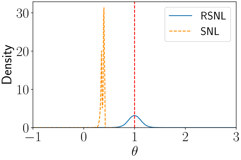
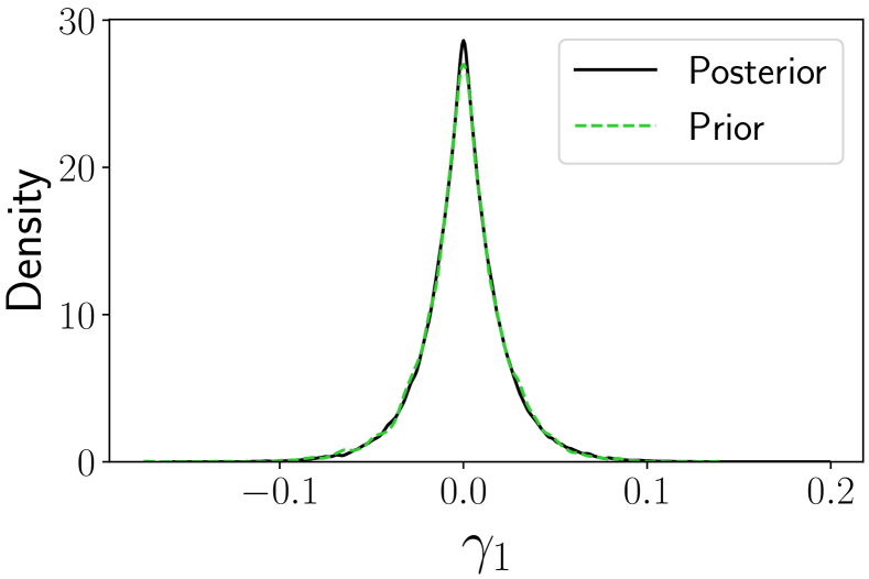
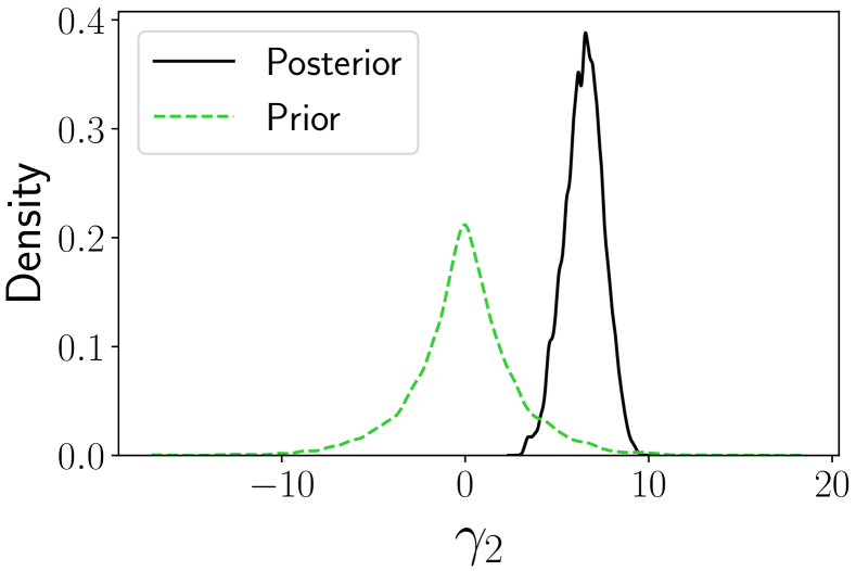
Figure 1: Posterior plots for the contaminated normal model. The leftmost plot shows the estimated univariate SNL (dashed) and RSNL (solid) posterior densities for $\theta$. The true parameter value is shown as a vertical dashed line. The right two plots show the estimated marginal posterior (solid) and prior (dashed) densities for the components of $\Gamma$.

It is evident in Figure 1 that RSNL gives reliable inference with high posterior density surrounding the true parameter value, $\theta=1$. In stark contrast, SNL gives unreliable inference with negligible support around the true parameter value.

Figure 1 also includes the posteriors for the components of $\Gamma$. For $\gamma_{1}$ (associated with the compatible summary statistic), the prior and posterior are effectively indistinguishable. This is consistent with the behaviour of RBSL. For $\gamma_{2}$ (associated with the incompatible statistic), the misspecification is detected since the posterior has high density away from 0. Visual inspection is sufficient here for the modeller to detect the misspecified summary and provides some insight to adjust the model accordingly. The introduction of additional auxiliary variables does not come with excessive computational costs. For this example, the total computation time for RSNL is around 40 minutes and for SNL is around 10 minutes.

4.2 Misspecified MA(1)

We follow the misspecified moving average (MA) of order 1 example in Frazier and Drovandi, (2021), where the assumed DGP is an MA(1) model, $y_{t}=w_{t}+\theta w_{t-1}$, $-1\leq\theta\leq 1$ and $w_{t}\overset{\text{i.i.d.}}{\sim}\mathcal{N}(0,1)$. However, the true DGP is actually a stochastic volatility model of the form:

$$y_{t}=\exp\left(\frac{z_{t}}{2}\right)u_{t},\quad z_{t}=\omega+\kappa z_{t-1}+v_{t}+\sigma_{v},$$

where $0<\kappa,\sigma_{v}<1$, and $u_{t},v_{t}\overset{\text{i.i.d.}}{\sim}\mathcal{N}(0,1)$. We generate the observed data using the parameters, $\omega=-0.76$, $\kappa=0.90$ and $\sigma_{v}=0.36$. The data is summarised using the autocovariance function, $\zeta_{j}(x)=\frac{1}{T}\sum_{i=j}^{T}x_{i}x_{i-j-1}$, where $T$ is the number of observations and $j\in\{0,1\}$ is the lag. We use the prior $\theta\sim\mathcal{U}(-1,1)$ and set $T=100$.

It can be shown that for the assumed DGP, $b(\theta)=(1+\theta^{2},\theta)^{\top}$. Under the true DGP, $b_{0}=(\exp(\frac{\omega}{1-\kappa}+\frac{\sigma_{v}^{2}}{2(1-\kappa^{2})}),0)^{\top}\approx(0.0007,0)^{\top}$. As evidently $\inf_{\theta\in\Theta}||b(\theta)-b_{0}||>0$, the model is misspecified as outlined in Section 2.2. We also have a unique pseudo-true value with $||b(\theta)-b_{0}||$ minimised at $\theta=0$. The desired behaviour for our robust algorithm is to detect incompatibility in the first summary statistic and centre the posterior around this pseudo-true value. As the first element of $b_{0}$ goes from $1\rightarrow 0$, $||b(\theta)-b_{0}||$ increases and the impact of model misspecification becomes more pronounced. We set $S(y)=(0.01,0)^{\top}$ as a representative observed summary from the true DGP to assess the performance of SNL and RSNL under heavy misspecification.

Figure 2 shows that RSNL both detects the incompatible sample variance statistic and ensures that the approximate posterior concentrates onto the parameter value that favours matching of the compatible statistic, i.e. $\theta=0$. SNL, however, is biased and has less support for the pseudo-true value.

As expected, $\gamma_{1}$ (corresponding to the incompatible statistic) has significant posterior density away from 0 as seen in Figure 2. Also, the posterior for $\gamma_{2}$ (corresponding to the compatible statistic) closely resembles the prior. The computational price of making inferences robust for the misspecified MA(1) model is minimal, with RSNL taking around 20 minutes to run and SNL taking around 10 minutes.

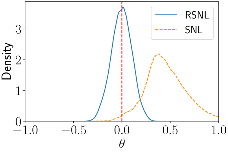
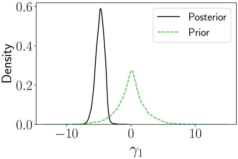
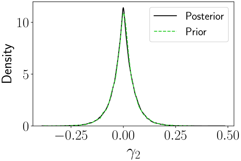
Figure 2: Posterior plots for the misspecified MA(1) model. The leftmost plot shows the estimated univariate SNL (dashed) and RSNL (solid) posterior densities for $\theta$. The true parameter value is shown as a vertical dashed line. The right two plots show the estimated marginal posterior (solid) and prior (dashed) densities for the components of $\Gamma$.

4.3 Contaminated SLCP

The simple likelihood complex posterior (SLCP) model devised in Papamakarios et al., (2019) is a popular example in the SBI literature. The assumed DGP is a bivariate normal distribution with the mean vector, $\mu_{\theta}=(\theta_{1},\theta_{2})^{\top}$, and covariance matrix:

$$\Sigma_{\theta}=\begin{bmatrix}s_{1}^{2}&\rho s_{1}s_{2}\\ \rho s_{1}s_{2}&s_{2}^{2}\\ \end{bmatrix},$$

where $s_{1}=\theta_{3}^{2}$, $s_{2}=\theta_{4}^{2}$ and $\rho=\tanh({\theta_{5}})$. This results in a nonlinear mapping from $\theta=(\theta_{1},\theta_{2},\theta_{3},\theta_{4},\theta_{5})\in\mathbb{R}^{5}\rightarrow y\in\mathbb{R}^{2}$. The posterior is “complex” having multiple modes due to squaring as well as vertical cutoffs from the uniform prior that we define in more detail later. Hence, the likelihood is expected to be easier to emulate than the posterior, making it suitable for an SNL type of approach. Four draws are generated from this bivariate distribution giving the likelihood, $g(y\mid\theta)=\prod_{j=1}^{4}\mathcal{N}(y_{j};\mu_{\theta},\Sigma_{\theta})$ for $y=(y_{1},y_{2},y_{3},y_{4})$. No summarisation is done and the observed data is used in place of the summary statistic. We generate the observed data at parameter values, $\theta=(0.7,-2.9,-1.,-0.9,0.6)^{\top}$, and place an independent $\mathcal{U}(-3,3)$ prior on each component of $\theta$.

To impose misspecification on this illustrative example, we draw a contaminated 5-th observation, $y_{5}$ and use the observed data $y=(y_{1},y_{2},y_{3},y_{4},y_{5})$. Contamination is done by applying the (stochastic) misspecification transform considered in Cannon et al., (2022), $y_{5}=x_{5}+100z_{5}$, where $x_{5}\sim\mathcal{N}(\mu_{\theta},\Sigma_{\theta})$, and $z_{5}\sim\mathcal{N}((0,0)^{\top},100\mathbb{I}_{2})$. The assumed DGP is not compatible with this contaminated observation, and ideally the approximate posterior would ignore the influence of this observation.

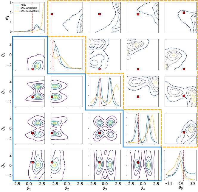
Figure 3: Univariate and bivariate density plots of the estimated posterior for $\theta$ on the SLCP example. Plots on the diagonal are the univariate posterior densities obtained by RSNL (solid) and SNL (dashed) on the contaminated SLCP example, and for SNL without the contaminated draw (dotted). The bivariate posterior distributions for contaminated SLCP are visualised as contour plots when applying RSNL (solid, lower triangle off-diagonal) and SNL (dashed, upper triangle off-diagonal). The true parameter values are visualised as a vertical dashed line for the marginal plots and the $\times$ symbol in the bivariate plots.

We thus want our inference to only use information from the four draws from the true DGP. The aim is to closely resemble the SNL posterior where the observed data is the four non-contaminated draws. Figure 3 shows the estimated posterior densities for SNL (for both compatible and incompatible summaries) and RSNL for the contaminated SLCP example. When including the contaminated 5-th draw, SNL produces a nonsensical posterior with little useful information. Conversely, the RSNL posterior has reasonable density around the true parameters and has identified the separate modes.

The first eight compatible statistics are shown in Figure 5. The prior and posteriors reasonably match each other. In contrast, the observed data from the contaminated draw is recognised as being incompatible and has significant density away from 0 as evident in Figure 5. Again, there is not a significant computational burden induced to estimate the adjustment parameters, with a total computational time of around 6 hours to run RSNL and around 4 hours for SNL.

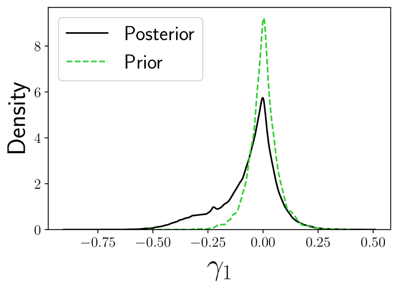
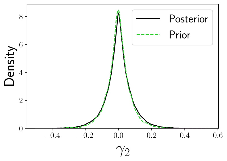
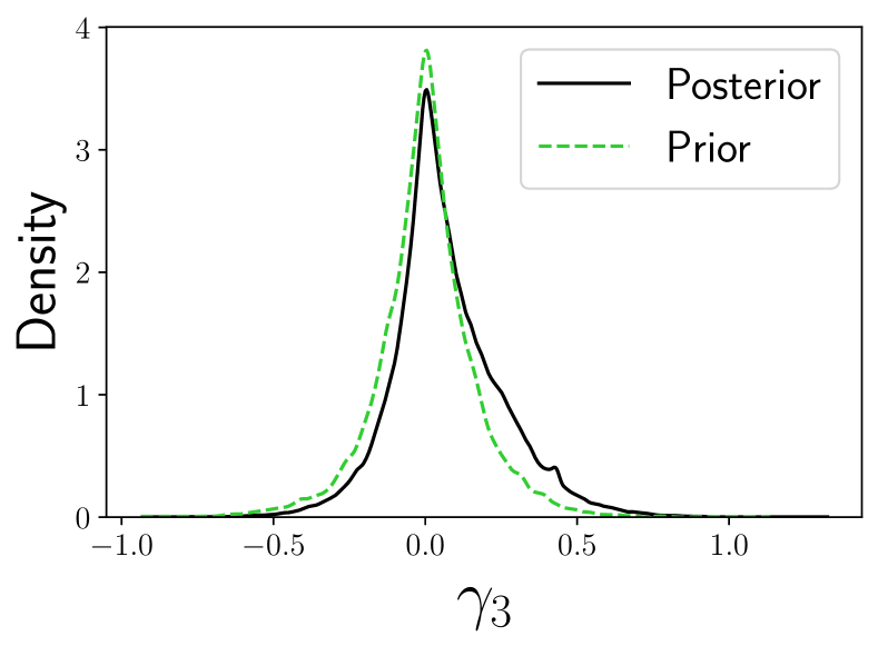
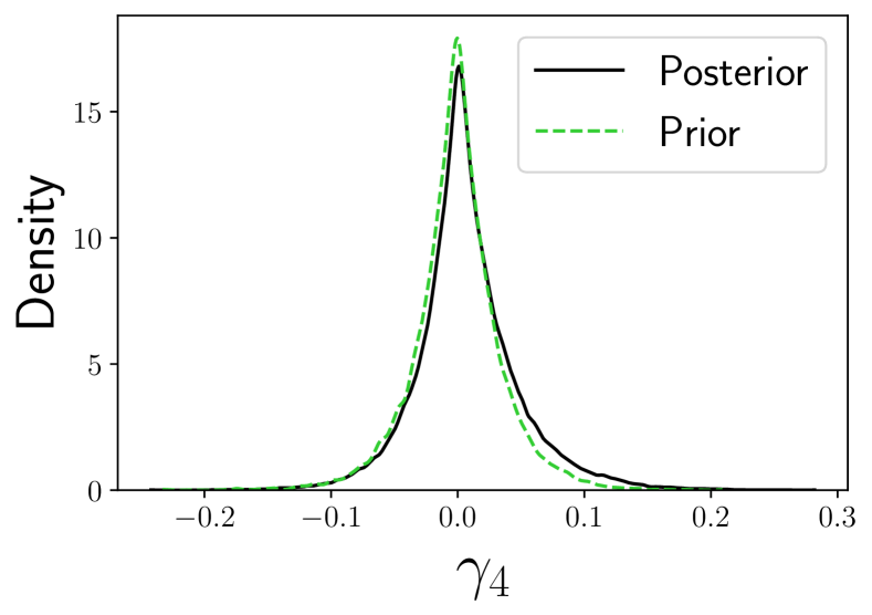
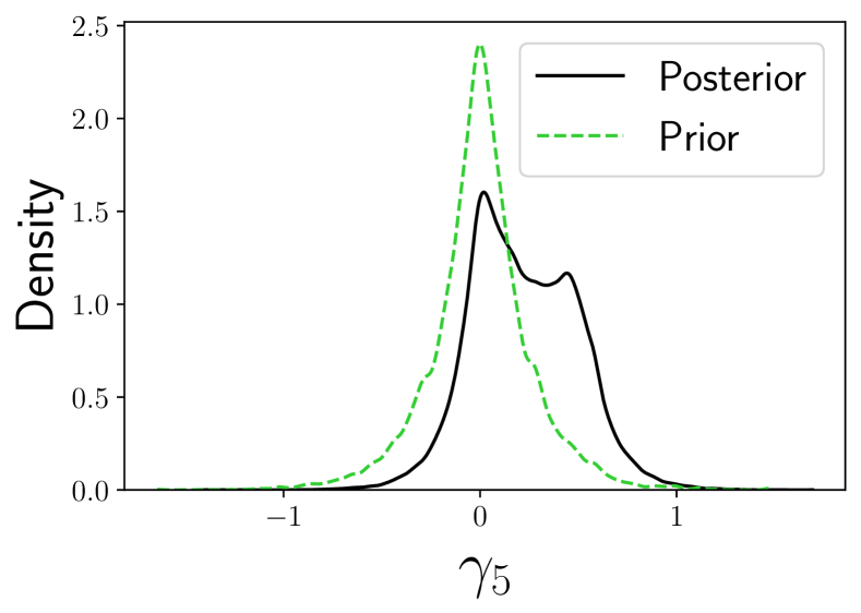
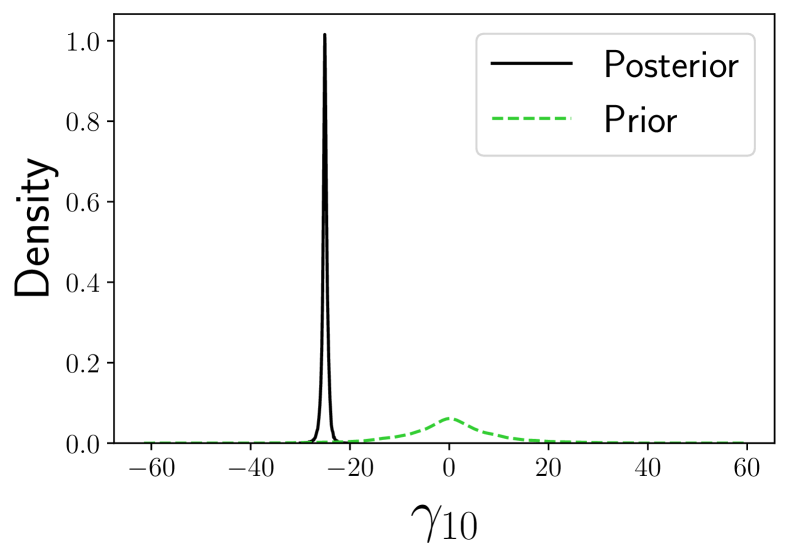
Figure 4: Estimated marginal posterior (solid) and prior (dashed) for components of $\Gamma$ corresponding with the non-contaminated draws.

Figure 5: Estimated marginal posterior (solid) and prior (dashed) for components of $\Gamma$ corresponding with the contaminated draw.

5 Discussion

In this work, we have introduced a new neural SBI method that is robust to model misspecification. To our knowledge, this is the first method that both detects and corrects for model misspecification that targets the likelihood or uses sequential sampling. RSNL was shown on several illustrative examples to be robust to model misspecification while still conducting efficient inference.

We have shown that RSNL can provide useful inference with a fraction of the number of simulation calls of ABC and BSL methods. For example, only 10,000 model simulations were run to produce the RSNL posterior for the contaminated normal model. In contrast, RBSL in Frazier and Drovandi, (2021) used in the order of millions of model simulations. A more rigorous comparison, such as the benchmarks in Lueckmann et al., (2021), could be done between ABC, BSL and neural SBI methods to ascertain their robustness to model misspecification and behaviour across different numbers of simulations. Such a benchmark would ideally include challenging applications with real-world data to demonstrate the utility of these methods for scientific applications.

In the mean adjustment approach of RBSL, Frazier and Drovandi, (2021) account for the different summary scales and the fact that these scales could be $\theta$-dependent by adjusting the mean using $\mu_{m}(\theta)+\sigma_{m}(\theta)\circ\Gamma$, where $\sigma(\theta)$ is a vector of estimated standard deviations of the model summaries at $\theta$. In RBSL, these standard deviations are estimated from the $m$ model simulations generated based on $\theta$. Analogously, we could consider a similar approach in RSNL and define the target

$$\pi(\theta,\Gamma\mid S(y))\propto q_{\phi}(S(y)-\sigma(\theta)\circ\Gamma\mid\theta)\pi(\theta)\pi(\Gamma).$$

The question then becomes, how do we estimate $\sigma(\theta)$ in the context of RSNL? In the MCMC phase we do not want to generate more model simulations as this would be costly. If we believed that the standard deviation of the model summaries had little dependence on $\theta$, we could set $\sigma(\theta)=\sigma=\sigma(\hat{\theta})$ where $\hat{\theta}$ is some reasonable point estimate of the parameter. Another approach would, for each $\theta$ proposed in the MCMC, estimate $\sigma(\theta)$ using surrogate model simulations generated using the fitted normalising flow. This would be much faster than using actual model simulations, but could still slow down the MCMC phase substantially. Instead of using a normalising flow, we could train a mixture density network (Bishop,, 1994) to emulate the likelihood, which would then lead to an analytical expression for $\sigma(\theta)$. A multivariate mixture density network could replace the flow completely, or the multivariate flow for the joint summary could be retained and a series of univariate mixture density networks applied to each summary statistic for the sole purpose of emulating $\sigma(\theta)$. We plan to investigate these options in future research.

One might be concerned that the inclusion of adjustment parameters will introduce noise into the estimated posterior to a deleterious extent. Empirically we have found this to have a negligible effect, especially for the considered prior choice. This is consistent with the findings for RBSL in Frazier and Drovandi, (2021). Additionally, Hermans et al., (2022) noted that SBI methods (including SNL) tend to produce overconfident posterior approximations. Hence, it seems unlikely that the small amount of noise from the adjustment parameters would result in overly conservative posterior estimates.

A modeller can determine what summaries are misspecified by comparing the prior and posterior densities for each component of $\Gamma$. We relied on visual inspection of the adjustment parameters for the presented examples. This could be tedious when considering a large number of summaries, and an automated approach could be considered instead.

Here we considered an adjustment approach through an MCMC sampling scheme as in Frazier and Drovandi, (2021). However, sequential neural variational inference (SNVI, Glöckler et al.,, 2022) can provide useful inference with a reduced number of model simulations compared to other sequential neural methods, such as SNL. SNVI targets either the likelihood or the likelihood-ratio, another common target in SBI (Durkan et al.,, 2020; Hermans et al.,, 2020)). Future work could investigate the impact of model misspecification on SNVI and to make SNVI robust through the incorporation of adjustment parameters. The adjustment could be to the likelihood as in RSNL, or through an adjustment approach that targets the likelihood-ratio.

The choice of $\pi(\Gamma)$ was found to be important in practice. Our prior choice was based on the dual requirements to minimise noise introduced by the adjustment parameters if the summaries are compatible, and to be capable of shifting the summary a significant distance from the origin if they are incompatible. The horseshoe prior is an appropriate choice for these requirements. Further work could consider how to implement this robustly in a NUTS sampler. Another approach is the spike-and-slab prior as in Ward et al., (2022). Further work is needed to determine the most appropriate prior.

The relation between model misspecification in SBI as in Frazier et al., (2020) and OOD data detection in machine learning (Yang et al.,, 2021) could be investigated more thoroughly. Cannon et al., (2022) obtained favourable results using OOD detection methods based on ensemble posteriors (mixtures of independent posteriors, Lakshminarayanan et al., (2017)) and sharpness-aware minimisation (Foret et al.,, 2021). Potentially the benefits of these OOD methods could be heightened when also using adjustment parameters.

References

- Andrieu and Roberts, (2009) Andrieu, C. and Roberts, G. O. (2009). The pseudo-marginal approach for efficient Monte Carlo computations. The Annals of Statistics, 37(2):697–725.
- Baydin et al., (2018) Baydin, A. G., Pearlmutter, B. A., Radul, A. A., and Siskind, J. M. (2018). Automatic differentiation in machine learning: a survey. Journal of Machine Learning Research, 18:1–43.
- Bingham et al., (2019) Bingham, E., Chen, J. P., Jankowiak, M., Obermeyer, F., Pradhan, N., Karaletsos, T., Singh, R., Szerlip, P. A., Horsfall, P., and Goodman, N. D. (2019). Pyro: Deep universal probabilistic programming. Journal of Machine Learning Research, 20:28:1–28:6.
- Bishop, (1994) Bishop, C. (1994). Mixture density networks. Working paper, Aston University.
- Boelts et al., (2022) Boelts, J., Lueckmann, J.-M., Gao, R., and Macke, J. H. (2022). Flexible and efficient simulation-based inference for models of decision-making. Elife, 11:e77220.
- Bon et al., (2022) Bon, J. J., Bretherton, A., Buchhorn, K., Cramb, S., Drovandi, C., Hassan, C., Jenner, A. L., Mayfield, H. J., McGree, J. M., Mengersen, K., Price, A., Salomone, R., Santos-Fernandez, E., Vercelloni, J., and Wang, X. (2022). Being Bayesian in the 2020s: opportunities and challenges in the practice of modern applied Bayesian statistics. To appear in Philosophical Transactions A.
- Bradbury et al., (2018) Bradbury, J., Frostig, R., Hawkins, P., Johnson, M. J., Leary, C., Maclaurin, D., Necula, G., Paszke, A., VanderPlas, J., Wanderman-Milne, S., and Zhang, Q. (2018). JAX: composable transformations of Python+NumPy programs. Python package version 0.3.13, URL https://github.com/google/jax.
- Cannon et al., (2022) Cannon, P., Ward, D., and Schmon, S. M. (2022). Investigating the impact of model misspecification in neural simulation-based inference. arXiv preprint arXiv:2209.01845.
- Cranmer et al., (2020) Cranmer, K., Brehmer, J., and Louppe, G. (2020). The frontier of simulation-based inference. Proceedings of the National Academy of Sciences, 117(48):30055–30062.
- Drovandi and Frazier, (2022) Drovandi, C. and Frazier, D. T. (2022). A comparison of likelihood-free methods with and without summary statistics. Statistics and Computing, 32(3):1–23.
- Durkan et al., (2019) Durkan, C., Bekasov, A., Murray, I., and Papamakarios, G. (2019). Neural spline flows. In Advances in Neural Information Processing Systems 32.
- Durkan et al., (2020) Durkan, C., Murray, I., and Papamakarios, G. (2020). On contrastive learning for likelihood-free inference. In The 37-th International Conference on Machine Learning, pages 2771–2781. PMLR.
- Foret et al., (2021) Foret, P., Kleiner, A., Mobahi, H., and Neyshabur, B. (2021). Sharpness-aware minimization for efficiently improving generalization. In International Conference on Learning Representations.
- Frazier and Drovandi, (2021) Frazier, D. T. and Drovandi, C. (2021). Robust approximate Bayesian inference with synthetic likelihood. Journal of Computational and Graphical Statistics, 30(4):958–976.
- Frazier et al., (2021) Frazier, D. T., Drovandi, C., and Nott, D. J. (2021). Synthetic likelihood in misspecified models: consequences and corrections. arXiv preprint arXiv:2104.03436.
- Frazier et al., (2018) Frazier, D. T., Martin, G. M., Robert, C. P., and Rousseau, J. (2018). Asymptotic properties of approximate Bayesian computation. Biometrika, 105(3):593–607.
- Frazier et al., (2022) Frazier, D. T., Nott, D. J., Drovandi, C., and Kohn, R. (2022). Bayesian inference using synthetic likelihood: asymptotics and adjustments. Journal of the American Statistical Association (In Press).
- Frazier et al., (2020) Frazier, D. T., Robert, C. P., and Rousseau, J. (2020). Model misspecification in approximate Bayesian computation: consequences and diagnostics. Journal of the Royal Statistical Society: Series B (Statistical Methodology), 82(2):421–444.
- Glaser et al., (2022) Glaser, P., Arbel, M., Doucet, A., and Gretton, A. (2022). Maximum likelihood learning of energy-based models for simulation-based inference. arXiv preprint arXiv:2210.14756.
- Glöckler et al., (2022) Glöckler, M., Deistler, M., and Macke, J. H. (2022). Variational methods for simulation-based inference. In International Conference on Learning Representations.
- Greenberg et al., (2019) Greenberg, D., Nonnenmacher, M., and Macke, J. (2019). Automatic posterior transformation for likelihood-free inference. In The 36-th International Conference on Machine Learning, pages 2404–2414. PMLR.
- Hermans et al., (2020) Hermans, J., Begy, V., and Louppe, G. (2020). Likelihood-free MCMC with amortized approximate ratio estimators. In The 37-th International Conference on Machine Learning, pages 4239–4248. PMLR.
- Hermans et al., (2022) Hermans, J., Delaunoy, A., Rozet, F., Wehenkel, A., Begy, V., and Louppe, G. (2022). A crisis in simulation-based inference? Beware, your posterior approximations can be unfaithful. Transactions on Machine Learning Research.
- Hoffman and Gelman, (2014) Hoffman, M. and Gelman, A. (2014). The No-U-Turn Sampler: Adaptively setting path lengths in Hamiltonian Monte Carlo. Journal of Machine Learning Research, 15(1):1593–1623.
- Jasra et al., (2019) Jasra, A., Jo, S., Nott, D., Shoemaker, C., and Tempone, R. (2019). Multilevel Monte Carlo in approximate Bayesian computation. Stochastic Analysis and Applications, 37(3):346–360.
- Kingma and Ba, (2015) Kingma, D. P. and Ba, J. (2015). Adam: A method for stochastic optimization. In Bengio, Y. and LeCun, Y., editors, The 3rd International Conference on Learning Representations, ICLR.
- Kirichenko et al., (2020) Kirichenko, P., Izmailov, P., and Wilson, A. G. (2020). Why normalizing flows fail to detect out-of-distribution data. In Advances in Neural Information Processing Systems 34.
- Lakshminarayanan et al., (2017) Lakshminarayanan, B., Pritzel, A., and Blundell, C. (2017). Simple and scalable predictive uncertainty estimation using deep ensembles. In Advances in Neural Information Processing Systems 31.
- Levi and Craiu, (2022) Levi, E. and Craiu, R. V. (2022). Finding our way in the dark: approximate MCMC for approximate Bayesian methods. Bayesian Analysis, 17(1):193–221.
- Lewis et al., (2021) Lewis, J. R., MacEachern, S. N., and Lee, Y. (2021). Bayesian restricted likelihood methods: Conditioning on insufficient statistics in Bayesian regression (with discussion). Bayesian Analysis, 16(4):1393–2854.
- Li and Fearnhead, (2018) Li, W. and Fearnhead, P. (2018). On the asymptotic efficiency of approximate Bayesian computation estimators. Biometrika, 105(2):285–299.
- Lueckmann et al., (2021) Lueckmann, J.-M., Boelts, J., Greenberg, D., Goncalves, P., and Macke, J. (2021). Benchmarking simulation-based inference. In The 24-th International Conference on Artificial Intelligence and Statistics, pages 343–351. PMLR.
- Marin et al., (2014) Marin, J.-M., Pillai, N. S., Robert, C. P., and Rousseau, J. (2014). Relevant statistics for Bayesian model choice. Journal of the Royal Statistical Society: Series B (Statistical Methodology), 76(5):833–859.
- Pacchiardi and Dutta, (2022) Pacchiardi, L. and Dutta, R. (2022). Score matched neural exponential families for likelihood-free inference. Journal of Machine Learning Research, 23.
- Papamakarios and Murray, (2016) Papamakarios, G. and Murray, I. (2016). Fast -free inference of simulation models with Bayesian conditional density estimation. In Advances in Neural Information Processing Systems 29.
- Papamakarios et al., (2021) Papamakarios, G., Nalisnick, E., Rezende, D. J., Mohamed, S., and Lakshminarayanan, B. (2021). Normalizing flows for probabilistic modeling and inference. Journal of Machine Learning Research, 22(57).
- Papamakarios et al., (2017) Papamakarios, G., Pavlakou, T., and Murray, I. (2017). Masked autoregressive flow for density estimation. In Advances in Neural Information Processing Systems 30.
- Papamakarios et al., (2019) Papamakarios, G., Sterratt, D., and Murray, I. (2019). Sequential neural likelihood: fast likelihood-free inference with autoregressive flows. In The 22nd International Conference on Artificial Intelligence and Statistics, pages 837–848. PMLR.
- Paszke et al., (2019) Paszke, A., Gross, S., Massa, F., Lerer, A., Bradbury, J., Chanan, G., Killeen, T., Lin, Z., Gimelshein, N., Antiga, L., Desmaison, A., Kopf, A., Yang, E., DeVito, Z., Raison, M., Tejani, A., Chilamkurthy, S., Steiner, B., Fang, L., Bai, J., and Chintala, S. (2019). PyTorch: An imperative style, high-performance deep learning library. In Advances in Neural Information Processing Systems 32.
- Phan et al., (2019) Phan, D., Pradhan, N., and Jankowiak, M. (2019). Composable effects for flexible and accelerated probabilistic programming in NumPyro. arXiv preprint arXiv:1912.11554.
- Price et al., (2018) Price, L., Drovandi, C. C., Lee, A., and Nott, D. J. (2018). Bayesian synthetic likelihood. Journal of Computational and Graphical Statistics, 27(1):1–11.
- Radev et al., (2022) Radev, S. T., Mertens, U. K., Voss, A., Ardizzone, L., and Köthe, U. (2022). Bayesflow: Learning complex stochastic models with invertible neural networks. IEEE Transactions on Neural Networks and Learning Systems, 33(4):1452–1466.
- Ratmann et al., (2009) Ratmann, O., Andrieu, C., Wiuf, C., and Richardson, S. (2009). Model criticism based on likelihood-free inference, with an application to protein network evolution. Proceedings of the National Academy of Sciences, 106(26):10576–10581.
- Schmitt et al., (2021) Schmitt, M., Bürkner, P.-C., Köthe, U., and Radev, S. T. (2021). Detecting model misspecification in amortized Bayesian inference with neural networks. arXiv preprint arXiv:2112.08866.
- Sharrock et al., (2022) Sharrock, L., Simons, J., Liu, S., and Beaumont, M. (2022). Sequential neural score estimation: likelihood-free inference with conditional score based diffusion models. arXiv preprint arXiv:2210.04872.
- Sisson et al., (2018) Sisson, S. A., Fan, Y., and Beaumont, M. (2018). Handbook of approximate Bayesian computation. CRC Press.
- Tejero-Cantero et al., (2020) Tejero-Cantero, A., Boelts, J., Deistler, M., Lueckmann, J.-M., Durkan, C., Gonçalves, P. J., Greenberg, D. S., and Macke, J. H. (2020). sbi: A toolkit for simulation-based inference. Journal of Open Source Software, 5(52):2505.
- Thomas et al., (2022) Thomas, O., Dutta, R., Corander, J., Kaski, S., and Gutmann, M. U. (2022). Likelihood-free inference by ratio estimation. Bayesian Analysis, 17(1):1–31.
- Vehtari et al., (2021) Vehtari, A., Gelman, A., Simpson, D., Carpenter, B., and Bürkner, P.-C. (2021). Rank-normalization, folding, and localization: an improved for assessing convergence of MCMC (with discussion). Bayesian Analysis, 16(2):667–718.
- Ward, (2023) Ward, D. (2023). flowjax. Python package version 7.0.0, [Online; accessed 17-January-2023], URL https://github.com/danielward27/flowjax.
- Ward et al., (2022) Ward, D., Cannon, P., Beaumont, M., Fasiolo, M., and Schmon, S. M. (2022). Robust neural posterior estimation and statistical model criticism. In Advances in Neural Information Processing Systems 35.
- Warne et al., (2018) Warne, D. J., Baker, R. E., and Simpson, M. J. (2018). Multilevel rejection sampling for approximate Bayesian computation. Computational Statistics & Data Analysis, 124:71–86.
- Warne et al., (2022) Warne, D. J., Prescott, T. P., Baker, R. E., and Simpson, M. J. (2022). Multifidelity multilevel Monte Carlo to accelerate approximate Bayesian parameter inference for partially observed stochastic processes. Journal of Computational Physics, 469:111543.
- Wiqvist et al., (2021) Wiqvist, S., Frellsen, J., and Picchini, U. (2021). Sequential neural posterior and likelihood approximation. arXiv preprint arXiv:2102.06522.
- Yang et al., (2021) Yang, J., Zhou, K., Li, Y., and Liu, Z. (2021). Generalized out-of-distribution detection: a survey. arXiv preprint arXiv:2110.11334.